Fluctuating Latttice, Several Scales

Fluctuating Lattice, Several Energy Scales

Abstract

In part I: We find a series physical scales such as 1) Planck scale, 2) Minimal approximate grand unification SU(5), 3) the mass scale of the see saw model right handed or Majorana neutrinoes, some invented scale with many scalar bosons, etc., and get the logarithms of these energy scales fitted by a quantity $q$ related to the dimensions of to the scales related dimensionalities of coefficients in Lagrangian densities, or some generalization of this $q$ to something similar in the various cases of the scales. The logarithm of the energies behave as a straight line versus the dimension related number $q$. This is being explained by an ontologically existing lattice, which fluctuates in lattice canstant $a$ fromplaceto place in space time or more precisely, it fluctuates quantum mechanically.

In Part II: We find a fitting of the three fine structure constants in the Standard Model by means of a no-susy and SU(5)-like - but only accurately SU(5) symmetric in the classical approximation - by means of three other parameters for each of which, however, we have speculative predictions: Quantum corrections due to the lattice which are three times as large as naive quantum corrections, because the lattice is supposed to lie in layers, one layer for each fermion-family; criticallity of the unified coupling, using the satnadrd model group $S(U(2)\times U(3))$; the unification scale is fitted inot the scale-system of part I.

Abstract

We suggest a model with a physical lattice for the gauge groups in the Standard Model with link variables taking values in the according to O´Raifeartaigh Standard Modelgroup, $S(U(2)\times U(3))$, and it is so similar to $SU(5)$, that in what we can call the classical approximation, it gives the same ratios between the three fine structure constants. But including quantum fluctuations[64, 65, 66] we get deviation from the GUT prediction, becuase there is not true $SU(5)$ and thus the true $SU(5)$ quantum fluctuations are lacking, unless they belong to the Standard-Model-group[31]. The remarkable thing is, that apart from just a factor 3 the deviations caused by these quantum fluctuations reproduce within uncertainties in the very accurately measured finestructure constants fit the data. The factor 3 we seek to explain by postulating that the truly existing lattice is really lying in three layers (as if we had three copies of the Standard model group, i.e. $SMG\times SMg\times SMG$).

Part I: Fluctuating Lattice, Relation between Scales
Part II: Approximate Minimal $SU(5)$, Fine Structure Constants

1 Overall Introduction

This article is composed of two parts, the first(review of [2]), in section 2, of which fits a series of energy scales, or we could say physical phenomena leading to a parameter (with dimension energy after we put $c=\hbar=1$) and thus potentially a/the “fundamental” energy scale, while the other part(review of [1]) section 3 could be considered an attempt to “rescue” grand unification SU(5) by interpreting it by being only an (accidental) classical approximation.

The overall plan will be so that we first discuss the many energy scales, in section 2, which we seek to unite by means of the model, which is a really existing lattice fluctuating in size.

Next comes the rescue of the Grand Unification[4, 5, 6] in section 3 by allowing it to be only a classical approximation[1, 42]; but then after that we return in section 4 to the attempt to unify the energy scales in the light, that it is really very much needed, because giving up the usually used susy[20, 62, 7] to make SU(5) GUT work points to lower unification energy scale than even the susy SU(5) unification, so that now the distance even in logarithm between the Planck scale and the unificationscale has become so large that it is hard to see how to make them compatible. Thus the call for our attempt to unify the scales by our fluctuating lattice[2] has got even more strong, than with usual susy unification.

The spirit of the present work is the attempt to get information about the underlying theory to be found by numerological scuccess from the information in the Standard Model parameters as counted in [35] or in other observations the right handed neutrino masses from neutrino-oscillations [3] or inflation [50, 49].

2 Introduction for first part: Energy Scales or Fluctuating lattice

To cure this fact we bring forward the idea of a truly existing lattice, which has wildly different sizes, of say the link length, in different places and/or in different components of a superposition. Really we think of the lattice as being superpositon of all possible deformations (which could be made by coordinate transformations/reparametrizations), so we can say we have in mind quantum fluctuations in reparametrizations, the gauge group of gravity.

In the tables in which we list the various energy scales we have attached to each scale a number $q$ or $n=4-q$, and the meaning is that $n$ should mean the power to which the inverse link size $1/a$ be raised in order to give weighting comming in in the calculation of the energy scale in question. In fact this means that for all the energy scales we have

“energy scale” $$\approx \sqrt[n]{<(1/a)^{n}>}$$ (1)

If the distribution in the fluctuating lattice had been very norrow this $n$ would make no difference, but assume and fit a very broad distrbution being a Gaussian distribution in $\ln a$,

$$P(\ln a)d\ln a = \frac{1}{2\pi\sigma}\exp(-\frac{1}{2\sigma}(\ln(a)-\ln(a_{0\;counting})^{2})d\ln(a)$$ (2)

where the spread $\sigma=5.5$ turns out[2], a rather large spread, when we have in mind that it is a spread in the logarithm. In first approximation we might think of a completely flat distribution in the logarithm. If there was scalings symmetry and we got the Haar measure distribution for the group of scalings with different factors, then we would get such a flat distribtuion in the logarithm $\ln(a)$. Actually you might think of (2) as a scalings symmetric distribution only weakly broken.

For the purpose of comparing with the $P_{vloume}(\ln(a))$ below we might write uding that density of hypercubes per unit four volume compared the one per density per four volume of a hypercube in the lattice is $1/a_{0\;counting}^{4}$. Using that we can write for the number of hypercubes in an infinitesimal region

$$P(\ln a)d\ln a = \frac{\frac{1}{2\pi\sigma}\exp(-\frac{1}{2\sigma}(\ln(a)-\ln(a_{0\;counting})^{2})}{a_{0\;counting}^{4}}d^{4}xd\ln(a).$$ (3)

2.1 Density definitions etc.

First let us be a bit more specific about how we think of this fluctuating lattice:

• Lattice in layers We imagine, that the lattice can lie in several layers compared to a simple Wilson lattice. An idea about having layers is best gotten by imagining, that we take a number , e.g. 3, Wilson lattices and have in nature all of them. Then for each fourvolume of the size of a hypercube in the lattice in space time we shall not have as in a simple Wilson lattice just one lattice site, but rather 3. We call this, that there are 3 layers. If the lattice fluctuate in size of the links and thus this size also varies of course from place to place in the Minkowski space time, we can in principle ask for such a number of layers in average for each size of link $a$. That is to say we can define a “numbers of layers for a small $a$ region ” = “ numbers of sites(or hypercubes) in the four volume of one single hypercube provided we count only hypercubes in a range of sizes $a$ given by say the infinitesimal $d\ln(a)$”

  $$P_{layer}(\ln(a))d\ln(a) =$$ “ numbers of hyper cubes with link-size (4)

  $$a^{\prime}\in\{a^{\prime}|a\leq a^{\prime}\leq a*\exp(d\ln(a))\}\hbox{ per four}$$

  volume $$a^{4} a$$ of the hypercubes for ”

  $$= \hbox{``Layer density''($a$)}d\ln(a)$$ (5)

• Density in Space Time Usually we consider of course densities per 4-volume of Minkowski (or the curved space time) space and then there is place in every layer for having $1/a^{4}$ four-cubes. So if the density of say sites per place for a four cube in one of layers say is per interval in the logarithm $d\ln(a)$ is $\hbox{``Layer density''}(a)d\ln(a)$ (and there are $1/a^{4}$ per $(unit\;length)^{4}$), then the density of sites per four volume in Minkowski space time is

  $$\begin{array}[]{r@{\;}l}P_{volume}(\ln(a))d^{4}xd\ln(a)&=\hbox{``Layer density''}(a)/a^{4}d^{4}xd\ln(a)\\ &=P_{layer}(\ln(a))/a^{4}d^{4}xd\ln(a)\\ \hbox{with ansatz (\ref{distrib})}:&=\frac{1}{2\pi\sigma}\exp(-\frac{1}{2\sigma}(\ln(a)-\ln(a_{0\;counting})^{2})/a^{4}d^{4}xd\ln(a)\\ &=\frac{1}{2\pi\sigma}\exp(-\frac{1}{2\sigma}(\ln(a)-\ln(a_{0\;counting})+4\sigma)^{2}+\\ &+4^{2}/2*\sigma-4\ln(a_{0\;counting}))d^{4}xd\ln(a)\\ \text{Calling}\ln(a_{0})&=\ln(a_{0\;counting})-4\sigma\\ \hbox{or }a_{0}&=a_{0\;counting}\exp(-4\sigma)\\ \hbox{then }\\ P_{volume}(\ln(a))d^{4}xd\ln(a)&=\frac{1}{2\pi\sigma}\exp(-\frac{1}{2\sigma}(\ln(a)-\ln(a_{0}))^{2}-\\ &-4^{2}\sigma/2-4\ln(a_{0}))d^{4}xd\ln(a)\\ &=\frac{1}{2\pi\sigma}\exp(-\frac{1}{2\sigma}(\ln(a)-\ln(a_{0}))^{2}-\\ &-8\sigma-4\ln(a_{0}))d^{4}xd\ln(a)\\ &=\frac{1}{2\pi\sigma}\exp(-\frac{1}{2\sigma}(\ln(a)-\ln(a_{0}))^{2})/a_{0}^{4}*\exp(-8\sigma)d^{4}xd\ln(a)\\ &=\frac{1}{2\pi\sigma}\exp(-\frac{1}{2\sigma}(\ln(a)-\ln(a_{0}))^{2})/a_{0\;counting}^{2}/a_{0}^{2}d^{4}xd\ln(a)\end{array}$$

  But if we should normalize properly this $P_{volume}(\ln(a))$ properly we should have had like in (3) that the division with $a_{0\;counting}^{2}a_{0}^{2}$ should be replaced by $a_{0\;counting}^{4}$. Thus the normalized $P_{volume}(\ln(a))$ looks rather

  $$P_{volume}^{(N)}(\ln(a))d\ln(a)d^{4}x/a_{0\;counting}^{4} = \frac{a_{0\;counting}^{2}}{a_{0}^{2}}P_{volume}(\ln(a))$$ (7)

  $$d\ln(a)d^{4}x/a_{0\;counting}^{4}$$

  $$= \exp(8\sigma)P_{volume}(\ln(a))$$

  $$d\ln(a)d^{4}x/a_{0\;counting}^{4}$$

This means that when we average over the distribution of the link length $a$ or this link length $a$ to some power $a^{p}$ say the answer is not the same as if we do it just averaging over links or hypercubes by their number. In fact denoting the two different averages $<..>_{counting}$ and $<...>_{volume}$ we find

$$<a^{p}>_{counting} = \int\frac{1}{2\pi\sigma}\exp(-\frac{1}{2\sigma}(\ln(a)-\ln(a_{0\;counting}))^{2})*a^{p}d\ln(a)$$ (9)

$$= \int\frac{1}{2\pi\sigma}\exp(-\frac{1}{2\sigma}((\ln(a)-\ln(a_{0\;counting}))^{2}-2p\sigma*\ln(a)))d\ln(a)$$

$$= \int\frac{1}{2\pi\sigma}\exp(-\frac{1}{2\sigma}(\ln(a)-\ln(a_{0\;counting}-\sigma*p)^{2}+$$

$$+p^{2}\sigma/2+p*\ln(a_{0\;counting}))d\ln(a)$$

$$= a_{0\;couning}^{p}\exp(p^{2}\sigma/2)$$ (10)

$$\hbox{so that }\sqrt[p]{<a^{p}>_{counting}} = a_{0\;counting}\exp(p\sigma/2)$$ (11)

$$\hbox{while }<a^{p}>_{volume} = a_{0}^{p}*\exp(p^{2}\sigma/2)$$ (12)

$$\hbox{so that }\sqrt[p]{<a^{p}>_{volume}} = a_{0}\exp(p\sigma/2).$$ (13)

$$\hbox{Of course }<a^{p}>_{volume} = \frac{<a^{p}/a^{4}>_{counting}}{<a^{-4}>_{counting}}$$ (14)

as checked: $$= \frac{a_{0\;counting}^{p-4}\exp((p-4)^{2}\sigma/2)}{a_{0\;counting}^{-4}\exp((-4)^{2}\sigma/2)}$$ (15)

$$= a_{0\;counting}^{p}\exp(p(p-8)\sigma/2)$$ (16)

$$= a_{0}^{p}\exp(p^{2}\sigma/2).$$ (17)

$$\hbox{Also:}\frac{\langle a^{p+b}\rangle_{counting}}{\langle a^{p}\rangle_{counting}} = a_{0\;counting}^{b}\exp((p+b)^{2}-p^{2})\sigma/2)$$ (18)

$$= a_{0\;counting}^{b}\exp(b(2p+b)\sigma/2)$$ (19)

$$\hbox{so that }\sqrt[b]{\frac{<a^{p+b}>_{counting}}{<a^{p}>_{counting}}} = a_{0\,counting}\exp(2p\sigma/2)*\exp(b\sigma/2)$$ (20)

$$= a_{0\;p}\exp(b\sigma/2)$$ (21)

$$= \sqrt{a_{0\;p}a_{0\;p+b}}$$ (22)

$$\hbox{where }a_{0\;p} = \hbox{Peak of }P_{layer}(\ln(a))*a^{p}$$ (23)

$$= \hbox{Peak of }\exp(-\frac{1}{2\sigma}(\ln(a)-\ln(a_{0\;counting})^{2}+p\ln(a))$$ (24)

$$= a_{0\;counting}\exp(p\sigma)$$ (25)

$$\hbox{so especially }a_{0} = a_{0\;p=-4}=a_{0\;counting}\exp(-4\sigma)$$ (26)

Let us especially learn that considering two averages of powers of the link variable in succession you get an increase by a factor

$$\frac{<a^{p+1}>_{counting}}{<a^{p}>_{counting}} = a_{0\;counting}\exp((p+1/2)\sigma).$$ (28)

So the effective energy scale when you work with powers of the link variable of the order of $p$ is about $a_{0\;counting}*\exp(p\sigma)$. So what we have to do to evaluate what the typicalpower is for the type of physics connected to the energy scale we want.

Basically our procedure is to represent the quantity, which we call the energy scale, as a root of or just the coefficient in the action or a ratio of such action related quantities, and then argue that this combination must - assuming no big (or small) numbers in other coupling or parmeters - that it should behave as the average of some power of the link length $a$, i.e. as say $<(1/a)^{n}>_{counting}=<a^{-n}>_{counting}$.

As just a repetition we used in the tables below also a to the power $n$ of $1/a$ equivalent number $q=4-n$,a notation inspired by considering the scales “see-saw” and “scalars” which are scales at which we postulate/speculate, that there are “a lot of” respectively fermion and boson masses. In fact we know that ignoring the interactions for simplicity the fermion and boson actions in field theory are

$$S_{fermion}=\int{\cal L}_{D}(x)d^{4}x = \int\bar{\psi}(x)(i\gamma^{\mu}\partial_{\mu}-m)\psi(x)d^{4}x+...$$ (29)

$$S_{scalar\;boson}=\int{\cal L}(x)d^{4}x = \int(\frac{1}{2}\eta^{\mu\nu}\partial_{\mu}\phi\partial_{\nu}\phi-\frac{1}{2}m^{2}\phi^{2})d^{4}x+...$$ (30)

and that the mass $m$ of the particle occurs in different powers $m^{q}$ for the two, namely $q=1$ forfermions and $q=2$ for bosons. For dimensional reasons these mass terms then - including the extra $1/a^{4}$ factor from number of hyper cubes going as $1/a^{4}$ in a unit space time - have link $a$ dependensies

mass term $$a \propto (1/a)^{4-q}.$$ dependence (31)

and so we have here $n=4-q$.

(Unfortunately we have in Part II used the letter $q$ for a non-integer quantity being the parameter for how much the finestructure constant deviate from the SU(5) prediction, which we predict to $q=3\pi/2$)

2.2 Our tables

Let us first deliver the table of the energy scales I included in the very workshop talk:

When we have to do with the quantities related to the scale being terms in lagrangians in a field theory, we have immediately a factor $1/a^{4}$ which means a $-4$ in the power.

It shall turn out from our fitting that the step in the energy scale per unit step in the power is a factor 251, which must then be identified with our step factor $\exp(\sigma)$.

Table of “Fundamental ?” Energy Scales

Name Energy value $n$ of $(1/a)^{n}$ q Coef. dim. Fit Lagrangian d. Planck scale $1.22*10^{19}$ 6 -2 -2 $2.44*10^{18}$GeV $\frac{1}{2\kappa}R$ reduced Planck $2.43*10^{18}$GeV 6 -2 -2 $2.44*10^{18}$GeV $\frac{1}{2\kappa}R$ Min. $SU(5)$ app. $5.3*10^{13}$GeV 4 0 0 $3.91*10^{13}$ GeV $-\frac{1}{16\pi\alpha}F_{\mu\nu}^{2}$ Susy SU(5) $10^{16}$ GeV 4 0 0 $3.91*10^{13}$ GeV -$\frac{1}{16\alpha}*F_{\mu\nu}^{2}$ See-saw $10^{11}$ GeV 3 1 1 $1.56*10^{11}$GeV $m_{R}\overline{\psi}\psi$ Fermion extrapolate $10^{4}$GeV 0 4 4 $10^{4}$ GeV “1”

Using $c=\hbar=1$,

“Reduced Planck” $$= \frac{1}{\sqrt{G_{Newton}*8\pi}}=2.43*10^{18}GeV$$ (32)

“unified (approximate) SU(5)” $$=$$ “where lines closest” (33)

$$= (say)5.3*10^{13}GeV$$

“see-saw” $$\sim$$ “typical right handed neutrino mass” (34)

$$\sim 10^{11}GeV.$$

The ‘scales” scalars and Fermion extrapolate also called “fermion tip” scale) are my inventions and need explanation later. ($\kappa=8\pi G=8\pi G_{Newton}$).

Next let me deliver the full table (from [2]) with scales which we now have found, including cases of scales judged by very good will:

Important to notice in this table is the very good fitting of our formula

“energy scale” $$= 10^{4}GeV*250^{n}$$ (35)

which is compared with the in the third column of the table. The fitted value is the lower one inside each block.

Name [Coefficient] “Measured” value Text ref. $n$ comming from Eff. $q$ in $m^{q}$ term Our Fitted value Lagangian dens. by status $1/a^{n}$ Planck scale $[mass^{2}]$ in kin.t. $1.22*10^{19}GeV$ 6 Gavitational $G$ q=-2 $2.44*10^{18}GeV$ $\frac{R}{2\kappa}$ wellknown $\kappa=8\pi G$ Redused Planck $[mass^{2}]$ in kin.t. $2.43*10^{18}GeV$ (32) 6 Gravitational $8\pi G$ q=-2 $2.44*10^{18}GeV$ $\frac{R}{2\kappa}$ wellknown $\kappa=8\pi G$ Minimal $SU(5)$ $[1]$ $5.3*10^{13}GeV$ (33) 4 fine structure const.s $\alpha_{i}$ q=0 $3.91*10^{13}GeV$ $\frac{F^{2}}{16\pi\alpha}$ only approximate $F_{\mu\nu}=\partial_{\mu}A_{\nu}-\partial_{\nu}A_{d\mu}$ Susy $SU(5)$ $[1]$ $10^{16}GeV$ 4 fine structure const.s q=0 $3.91*10^{13}GeV$ $\frac{F^{2}}{16\pi\alpha}$ works $F_{\mu\nu}=\partial_{\mu}A_{\nu}-\partial_{\nu}A_{\mu}$ Inflation $H$ $[1]?$ $10^{14}GeV$ 4 CMB, cosmology q=0? $3.91*10^{13}GeV$ $\lambda\phi^{4}$ “typical” number $V=\lambda\phi^{4}$ Inflation $V^{1/4}$ concistence ? $10^{16}GeV$ 5 CMB, cosmology q=-1? $9.96*10^{15}GeV$ consistency “typical” $V=\lambda\phi^{4}$? See-saw $[mass]in\;non-kin.$ $10^{11}GeV$ (34) 3 Neutrino oscillations q=1 $1.56*10^{11}GeV$ $m_{R}\bar{\psi}\psi$ modeldependent $m_{R}$ right hand mass Scalars $[mass^{2}]in\;non-kin.$ $\frac{seesaw}{44\;to\;560}$ 2 small hierarchy q=2 $\frac{1.56GeV}{250}$ $m_{sc}^{2}|\phi|^{2}$ invented by me breaking $\frac{seesaw}{scalars}$ Fermion tip $``[mass^{4}]in\;non-kin.^{\prime\prime}$ $10^{4}GeV$ 0 fermion masses q=4 $10^{4}GeV$ “1” extrapolation quadrat fit Monopole $``[mass^{5}]in\;non-kin.^{\prime\prime}$ $28GeV$ -1 dimuon 28 GeV q=5 $40GeV$ $m_{monopol}\int ds$ invented $S\propto a$ String $1/\alpha^{\prime}$ $``[mass^{6}]in\;non-kin.^{\prime\prime}$ $1Gev$ -2 hadrons q=6 $0.16GeV$ Nambu Goto intriguing $S\propto a^{2}$ String $T_{hagedorn}$ $`[mass^{6}]$ in  non-kin.” $0.170GeV$ -2 hadrons q=6 $0.16GeV$ Nambu Goto intriguing Domain wall “$[mass^{7}]$ in   non-kin.” $8MeV$ -3 dark matter q=7 $0.64MeV$ twobrane vol. far out

After the Bled I found several new scales that in fact quite remarkably fitted in rather well. In the recent articel arXiv:2411.03552 [hep-ph] [2] I extended the table of scales fitting to by the scales “monopoles” and “strings” for which we what would be with the fluctuating lattice the scales for monopole masses and for the string tension or say the Regge slope in the Veneziano model, when one estimate the actions for a single monopole or for a single string in our scheme. Quite surprisingly the string scale turning out is the one for hadronic strings with which historically string theory were first proposed. The monopole mass scale turns out not so far from the mass of two-muon resonance[54] with 28 GeV mass, which is one of the very few peaks found not belonging to the Standard Model in LHC.

Our fitting of the curve of scales by a linear function as function of the power $n$ may be presented as

“energy scale” $$= 10^{4}GeV*250^{n}$$ (36)

$$\hbox{or }log_{GeV}(\hbox{``energy scale''}) = 4+2.40*n(+logGeV)$$ (37)

$$\hbox{or }\ln_{GeV}(\hbox{``energy scale''}) = 9.21+5.53*n(+\ln GeV)$$ (38)

Different “Energy-scales” versus n = 4 -$(\pm)$“Coupling dimension”

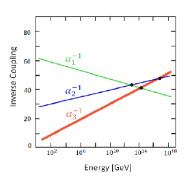
Figure 1: If I do not believe Susy, just look where lines closest. This is the usual plot of the running inverse fine structure constants normalized with the usual 3/5 on the U(1) coupling, so that they should have met in one point all three if exact SU(5) GUT had worked. But now we here refuse to believe in susy and instead assume the SU(5) symmetry only to be an approximate symmetry (see more in Part II) we take the energy (which is on the abscissa) at which the the three inverse fine structure constant curves are the closest to be the approximate unification scale. In our work [1] we found by more accurate lattice model assumptions $5.3*10^{13}GeV$ for the approximate unification scale. This approximate unification scale is indicated on the figure by a vertical line.

• There is a physically existing lattice, and the Plaquette action happens classically to be SU(5) symmetric.

• Quantum corrections break the classical SU(5) symmetry of the lattice action.

• Because the lattice lies in three layers, the quantum correction SU(5) breaking is just a factor 3 bigger than true quantum correction. The factor 3 is the number of families.

We shall return to this model of an only approximate grand unification SU(5) in the second part 3.

Since the power $n$ to which the inverse link length $a$ comes into the action $S$ for the Lagrangian densities for the different sort of physics related to the different (fundamental?) energy scales, $(1/a)^{n}$, is linearly related to the dimension of the coefficient [“coefficient”]

$$n = 4-(\pm)Dim(``Coefficient^{\prime\prime}),$$ (39)

linearity - i.e. straight line - of the logarithm of the energy scales as function of $n$ means also, that we observed straihgt line for the relation of Dim(“coefficient”) to logarithm(“energy scale”)

2.3 Fluctuating Lattice

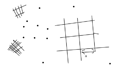
Figure 2: Here we drew for simplicity and easiness a couple of seperate pieces of lattices (two dimensional but of course they should really have been 4 dimensional to be in Minkowski space) of different lattice constant $a$ length and thus density. Meant is, however, that the lattice hangs together and that the link length varies along as one goes fromplace to place, presumably in a continuous way. Raelly it quantum fluctuates.

For the distribution of different densities of links or of sites in a fluctuating lattice with shall distinguish:

$$\#layers = (say)\;\#sites\;\hbox{per }a^{4}$$ (40)

$$density_{/m^{4}} = \#sites\;\hbox{per }m^{4}$$ (41)

$$density_{/m^{4}} = \#layers*a^{-4}$$ (42)

Ansatz:

Probability: (43)

$$P(\ln(1/a))d\ln(1/a)d^{4}x \propto$$

$$\propto\exp(-\frac{(\ln(1/a)-\ln(10^{4}GeV))^{2}}{2\sigma}) d\ln(1/a)d^{4}x$$ (44)

where $10^{4}GeV$ is our “fitted” value; $\sigma$ is a spreading to be fitted.

Distribution of Contribution for one of the to Scales associated actions versu $\ln(a)$

One of the actions associated with the candidates for fundamental scales as e.g. the Einstein-Hilbert-action $\frac{1}{2\kappa}R\sqrt{-g}d^{4}x$ with $(1/a)^{n}$ proportional contribtuion get of the form:

$$S= \int{\cal L}(x)d^{4}x\propto$$

$$\propto \int\exp(\frac{-(\ln(1/a))-\ln(10^{4}GeV))^{2}}{2\sigma})(1/a)^{n}d\ln(1/a)$$

$$= \exp(\frac{-(\ln(1/a)-\ln(10^{4}GeV))^{2}+n*2\sigma*\ln(1/a)}{2\sigma})d\ln(1/a)$$

An Action depends on the spread $\sigma$ like:

$$S = \int{\cal L}(x)d^{4}x\propto$$

$$\propto \int\exp(-\frac{(\ln(1/a))-\ln(10^{4}GeV)-n*\sigma)^{2}+(n*\sigma)^{2}}{2\sigma})d\ln(1/a)$$

$$= \int\exp(-\frac{(\ln(1/a))-\ln(10^{4}GeV))^{2}+(n*\sigma)^{2}}{2\sigma})d\ln(1/a)$$

$$= \int\exp(-\frac{(\ln(1/a))-\ln(10^{4}GeV))^{2}}{2\sigma})d\ln(1/a)*\exp(n^{2}\sigma/2)$$

where only the last factor $\exp(n^{2}*\sigma/2)$ depends on $n$. This was for an action $S\propto(1/a)^{n}$.

Interpreting the factor $\exp(n^{2}\sigma/2)$ as correcting the $n$ factors $(1/a)$ we get $(1/a)_{eff}=(1/a)*\exp(n\sigma)$.(because a step in $n^{2}\sigma/2$ is say $(n+1)^{2}\sigma/2-n^{2}\sigma/2=(2n+1)\sigma/2\approx n\sigma$).

We shall interprete correction to the effective $1/a$ (= the inverse of the link size) as a correction of the “energy scale”. So the effect of the spreading with Gauss distribution in the logarithm $\ln(1/a)$ with a width given by $\sigma$ as

Replace “energy scale” $$\rightarrow \hbox{``energy scale''}*\exp(n*\sigma)$$ (45)

$$\hbox{So }250 = \exp(\sigma/2)\hbox{(where $250$ from our empirical fit)}$$

$$\hbox{and thus }\sigma = 5.5.$$ (46)

2.4 Conclusion of Energy Scales and Fluctuating Lattice Part/First Part

• We presented an emprical straight line fit to three wellknown energy scales, valid to crude order of magnitude accuracy,

  “energy scale” $$= 10^{4}GeV*250^{n}$$ (47)

  or “energy scale” $$= 10^{4}GeV*250^{4-(\pm)dim(coefficient)}$$ (48)

  (where $dim(coefficient)$ is the dimension in energy units of the coefficient multiplying in the Lagrangian density the field (product), and $(\pm)=+1$ for the term with the coefficient being a mass term like in the case of the “see-saw”and the “scalars scale”, while in the case of “Plack scale” where it iis the Einstein Hilbert action, which is a kinetic term carrying a dimension 2 coefficient $(\pm)=-1$ )

• We explain this empirical fit with a speculated “fluctuating lattice” with a fluctuation distribution being a Gauss distribultion in the logarithm of the statistically fluctuating link length $a$, i.e. a Gauss distribution in $\ln(1/a)$:

  $$P \propto \exp(-\frac{(\ln(1/a)-\ln(10^{4}GeV)^{2}}{2*5.5}).$$ (49)

2.4.1 Last moment development

After the talk I found several new ideas for new scales (mainly) of the type that one considers a brane of some dimension $D$, meaning a space time extension of dimension $D+1$, and thus having an action, which using dimensionless parameters to makecoordinates on the brane-time-track, acoefficient of dimension like $a^{D+1}$ being $[energy^{-D-1}]$, so that $d=-D-1$. Very interesting it seems that for a string = (D=1)brane the tension of the strings pointed to by our extrapolated fit to $d=-2$ get very close to the tension of the string by which hadrons can crudely be fitted, and which were the historically starting point of string theory.

A plot with the extended system of scales is found in [2] and is reproduced in the figure 3.

Figure 3: This figure taken from [2] has the logarithm in basis 10 of the energy scales on the abscissa, and the intger $q=4-n$, where $n$ is esssentially the power of $1/a$ relevant for the scale. Remark that we have $-q$ as the variable pointing upwards. The names we have given to the scales are attached.

3 Approximate GUT SU(5)

part II: Approximate SU(5), Fine Structure Constants

Abstract for Second part: “Approximate $SU(5)$, Fine structure constants”

3.1 Introduction to approximate SU(5)

Shall fit with[1]

• $q=\hbox{``number of families''}*\pi/2$.

• $\alpha_{5\;uncorrected}=\alpha_{5\;critical}$ (unifying coupling (ours)).

• We shall put our replacement for unification energy scale $\mu_{U}$ into aline of four different energy scales, fitting a line in the logarithm of the energy scale versus dimension of related couplings.

Since our replacement for the unification coupling scale is even more deviating from the Planck scale than more popular unifications with susy[susy], we give up that the various “ fundamental scales found, see saw, unification (or approximate unification) and Planck scale, should be at the same energy. Rather we allow them to vary in a systematic way with the dimensionality of the related coefficients in the Lagrangian in the quantum field theory.

We interpret this fitting with a model of a truly existing lattice (probably irregular) which is fluctuating both in size and local shape, in a way corresponding to a fluctuation in the reparametrization gauge of general relativity. We though assume that it is somehow cut off so that the distribution of the link length say fluctuate on a logarithmic scale much like a Gaussian distribution in the logarithm.

Crossing in one point of Minimal $SU(5)$ Running (inverse) Fine structue constants not perfect.

Figure 4: This is the usual graph representing the three Standard Model inverse fine structure constants with the $\alpha_{1}^{-1}$ being in the notation suitable for $SU(5)$, meaning it is 3/5 times the natural normalization, $\alpha_{1\;SU(5)}^{-1}$ =$3/5*\alpha_{1\;SM}^{-1}$ =$3/5*\alpha_{EM}^{-1}cos^{2}\Theta_{W}$. The vertical thin line at the energy scale $\mu_{U}=5*10^{13}GeV$ points out “our unified scale”, which is as can be seen not really unifying the couplings, but rather is the scale where the ratio of the two independent differences, $\alpha_{2}^{-1}-\alpha_{1\;SU(5)}^{-1}$ and $\alpha_{1\;SU(5)}^{-1}-\alpha_{3}^{-1}$ have just the ratio 2/3 as our model predicts at the “ our unification scale”. One may note, that this “our unified scale” is actually very close to, where the three inverse couplings are nearest to each other, and in that sense an “approximate” unification scale.

Our prediction of Deviation from $SU(5)$.

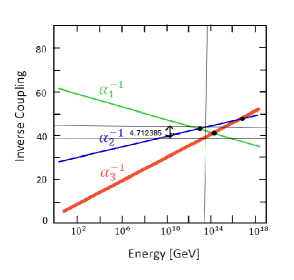
Figure 5: Same as figure 1, but now with our prediction inserted, marked as the number $4.712385=3*\pi/2$, which is predicted to be at the “our unified scale” the difference $1/\alpha_{2}-1/\alpha_{3}$. Our prediction is, that just at horizontal thin black line, at $5*10^{13}GeV$, corresponding to the scale $\mu_{U}$, given by our fitted to the green line crossing point dividing the region between the blue and the red in the ratio 2 to 3, we shall have the difference in ordinate between the red and the blue crossing points with the vertical black being $3\pi/2$.

(see [1] for the details and argument)

The three standard model fine structure constants (inverted):

$$\frac{1}{\alpha_{1\;SU(5)}(\mu_{U})} = \frac{1}{\alpha_{5\;uncor.}}-11/5*q$$ (50)

$$\frac{1}{\alpha_{2}}(\mu_{U}) = \frac{1}{\alpha_{5\;uncor.}}-9/5*q$$ (51)

$$\frac{1}{\alpha_{3}(\mu_{U})} = \frac{1}{\alpha_{5\;uncor.}}-14/5*q,$$ (52)

where the one parameter $\frac{1}{\alpha_{5\;uncor.}}$, is essentially the unified coupling, although we do not have unification proper.

The deviations come as quantumcorrections on the lattice - the fluctuation of the link-variables - sometimes refered to as “tachyon”[tachyon, 65].

$$\frac{1}{\alpha_{5\;cor.}} = \frac{1}{\alpha_{5\;uncor.}}-24/5*q.$$ (53)

The other parameter $q$ we believe to have calculated in our model with its 3 families of fermions and in a Wilson lattice in a lowest order approximation:

$$q = ``\#families^{\prime\prime}*\pi/2=3*\pi/2=4.712385.$$ (54)

Using this notation we could equally well use the formulation

$$\frac{1}{\alpha_{1\;SU(5)}(\mu_{U})} = \frac{1}{\alpha_{5\;cor.}}+13/5*q$$ (55)

$$\frac{1}{\alpha_{2}(\mu_{U})} = \frac{1}{\alpha_{5\;cor.}}+3*q$$ (56)

$$\frac{1}{\alpha_{3}(\mu_{U})} = \frac{1}{\alpha_{5\;cor.}}+2*q.$$ (57)

Table of Fitting the Three parameters

Parameter Formula From $\alpha$’s Theory Deviation Section q q=$1/\alpha_{2}(\mu_{U})-1/\alpha_{3}(\mu_{U})$ 4.618 4.712385 -0.094$\pm$0.05 LABEL:ps3, LABEL:dbausu5 $1/\alpha_{5\;uncor.}(\mu_{U})$ see above 51.705 45.927 5.778$\pm$ 3.5 LABEL:ps10 $\ln(\frac{\mu_{U}}{M_{Z}})$ $\ln(\frac{\mu_{U}}{m_{t}})=\frac{2}{3}*\ln(\frac{E_{Pl\;red}}{M_{t}})$ 27.04 24.76 2.28$\pm$ 1 LABEL:scale or 0.02

In the third line we now replace the top mass $m_{t}$ with a mass value gotten by extrapolating from the whole spectrum of quarks and leptons, which is about $10TeV$ and the agreement got very good indeed.

3.2 Model

We assume ANTI-GUT: Diagonal subgroup breaking
[26, 12, 11, 13, 14, 15, 16, 18]

$$G_{full} = SMG\times SMG\times SMG$$ (58)

$$\hbox{where }SMG = S(U(1)\times U(3))$$ (59)

$$= ({\bf R}\times SU(2)\times SU(3))/{\bf Z}_{app}$$ (60)

where

$${\bf Z}_{app} = \left\{(r,U_{2},U_{3})|\right.$$

$$\left.\exists n\in{\bf Z}[(r,U_{2},U_{3})=\left(2\pi,-{\bf 1},\exp(i2\pi/3){\bf 1}\right)^{n}]\right\}$$

$$SMG_{as\;observed} = \{(g,g,g)|g\in SMG\}\subset G_{full}$$ (61)

It is our crucial assumption that we have a lattice theory with plaquette-action given proportional to the trace of the representative of the plaquette group element $U_{Pl}(\Box)$ in the/a “smallest” representation[28, 30, 29] - taken here as the representation in the five-plet $SU(5)$ representation ${\bf 5}$:

$$\rho(U_{pl}(\Box) : {\bf 5}\rightarrow{\bf 5}$$ (62)

$$\hbox{or }\rho(U_{pl}(\Box)) \in UnitaryMarix(5\times 5)$$ (63)

We have once pointed out that the very standard model group $SMG$ is selected[28, 29, 30] as the one having with appropriate definition the smallest relative to the group faithful representation.

To get a predition for the unified coupling at the approximate unification scale we make the assumption that somehow the coupling constants at this scale becomes just couplings which are“critical”in the sense of seperating typically several phases of the lattice theory. We call this assumption “multiple point criticallity principle”(MPP)[13, 14, 15, 16, 17, 18].

3.3 Fitting

Taking our $q=3\pi/2$ as just given in our model, and we predict the differences from a to be fitted “unified” inverted coupling $1/\alpha_{5\;uncor.}$ at a to be fitted “unification scale” $\mu_{U}$, we really only provide one predicted parameter at first. Really we predict the two independent differences, say $1/\alpha_{2}-1/\alpha_{3}=q$ and $1/\alpha_{2}-1/\alpha_{1\;SU(5)}=2/5*q$ at the “unification scale”.

E.g. select the scale by having the ratio of the two differences the predicted one; then the absolute size is a true prediction.

We got $q=4.6$ by the fine structure constant data and the $3\pi/2=4.712$.

Inverse Fine structure constants at the $\mu_{U}$-scale

Figure Caption about Critical Coupling
[21, 22, 23, 14, 13, 11]

Explaing figure:The axis is the axis of inverse fine structure constants; The group names U(1), SU(2) and Su(3) are the by renormalization group to the replacement of unification scale $\mu_{U}$ extrapolated expeimental inverse fine structure constants for these groups respectively. The two $SU(5)$ inverse fine structure constants are repectively with and without the quantum fluctuation contribution.

To justify that the above figure implies that the unified coupling represented by the inverse fine structure constant has indeed the critical value (for a phase transition, presumably between confinement or not) we make use of the following three approximations/assumptions:(see next slide)

• The critical couplings for a true $SU(5)$ lattice theory and for the Standard Modelgroup[31, 28, 29, 30] deviate only little, because the standard model group can be considered an attenuation of the SU(5) one.

• We can trust a rather simple formula [9, 62] for the critical couplings for the SU(N) groups,

  $$\frac{1}{\alpha_{N}} = \frac{N}{2}\sqrt{\frac{N+1}{N-1}}\alpha_{U(1)crit}^{-1}$$ (64)

  $$\hbox{where }\alpha_{U(1)crit}^{-1} = 0.2\pm 0.015$$ (65)

  found in an article with Laperashvili and others[62].

• The critical coupling for the Standard Model group $S(U(3)\times U(2))$ should be compared to couplings with equally many quantum fluctuation contributions as it has itself.

And then the assumption of the model which is not only an approximation:

We compare the “ unified couplings” not to simply the critical one but the by a factor 3 weakened one, so that we have multiplied the critical inverse finestructure constant for the Standard Model group by 3, to compareit with the unified couplings.(the 3 is again the number of families)

4 Gravity Problem; Return to First Part again

Return to Part I: on the scales in fluctuating lattice model

Really I believe that gauge symmetries could be due to very huge fluctuations in thosedegreesof freedom which arethe guage-monters.

If a lattice were connected to a coordinate system in general relativity, but the guage not fixed but allowed to fluctuate[NNF], we should get a lattice fluctuating relative to what we would consider the fixed geometry.

Contributions as function of ln scale in fluctuating lattice:

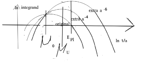
Figure 6: Shifted Scales Depending on Weighting with $(1/a)^{n}$ weight factor: On the abscissa we have the logarithm $\ln(1/a)$ of energy $1/a$, and for several cases of weighting with powers of the $1/a$ we have on the ordinate the logarithm of the contribtuion density to the average of these powers of $1/a$. In the Gauss distribution assumption, which we use the logarithm of the distribution density as function of the $\ln(1/a)$ is a parbola (pointing dowward) and for the various powers of $1/a$ shown the weighted distribution becomes again a now displaced parabola. It is the displacement component along the abscissa here, which represents the change in effective energy scale, which is the central effect dicussed in the first part of this paper.

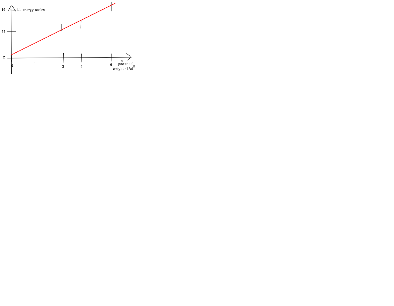
Figure 7: Here we attempted to fit our first four energy scales with the “fermion tip” scale approximated by just the top mass $m_{t}$, because of course after all the top quark is the heaviest, so it is approximately the tip scale. On the abscissa we have the energy scale characteristic integer $n$ essentially denoting which power $(1/a)^{n}$ is relevant for the energy scale in question. The ordinate is the logarithm with basis 10 of the energy scale. We use base 10, because it makes it easier to relate to our ten-power notation for the energy scales.

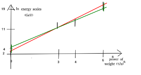
Figure 8: However, taking for the “fermion tip” scale rather than just top mass $m_{t}$ the value gotten by the extrapolation $m_{mnl}$ as seen in figure 9 and in the tables for respectively quarkmasses and leptonmasses not long below. The fitting is a bit better than for using the top-mass simply.

The plot of scales versus weighting power $n$

We present 4 energy scales of physical interest together with lattice link size $a$ dependent factor comming into the expression in the action or Lagrangian relevant for the scale in question. It is essentially the dimension of the termin the Lagrangian density without counting the coefficient (so it is rather trivially related to this coefficient). We took:

• 0 $(1/a)^{0}$ This scale is the scale of maximal number of “active”/effectively massless families. (Needs more explanation below.). Below extrapolation $\sim 10TeV$.

• 3 $(1/a)^{3}$ The see-saw neutrino mass scale

• 4 $(1/a)^{4}$ The our “unification scale”,at which the Yang Mills theories are supposed to be given by the truly existing fluctuating lattice.

• 6 $(1/a)^{6}$ The Planck scale, related to the Einstein-Hilbert-action.

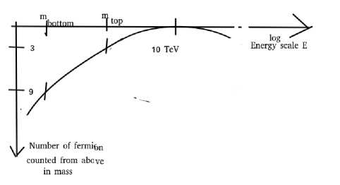
Figure 9: Fitting Weyl Fermion masses by number after mass by Philosophy of Fluctuating Lattice: In order to make an as good as possible extrapolation to where the series of masses of the fermions in the Standard Model we should assume how this series of masses is related to some ansatz formula for their density on say the logarithm of mass axis. Inspired by our ideas of a fluctuating lattice with a Gaussian conbined with a connection of the number of fermions with relative to that scale negligible mass being proportional to the layer density at the scale, we suggested: The number of a fermion counted from the heaviest, the next heaviest, etc. should be approximately proportional to the square of the distance in logarithm from the “extrapolated tip” of the mass region, which we call $m_{mnl}$ to the massoof the fermion. On this plot we see as function of the logarithm of masses the number in the series counted from the heaviest down according to mass. We have let the axis denoting the number in the series point down. So the curve is to be fitted by a (half) parabla.

Quark for $m_{mnl}=10^{4}GeV$

$m_{mnl}$ = “maximum number of layers” is the energy scale at which density of the distributuion of inverse lattice sizes $1/a$ is the biggest.

We fit to this density being proportional to the number of Weyl fermions relative to the scale being light/massless. Since the last column $diff^{2}/n$ fits a constant 1.12 to about 0.1 we have good fit for the 10 TeV.

Name number $n$ Mass $m$ $log_{10\;GeV}m$ $diff$=$4-logm$ $diff^{2}$ $diff^{2}/n$ top 3$\pm$ 1 172.76 $\pm$ 0.3 GeV 2.2374$\pm$ 0.0008 1.7626 3.1066$\pm$ 0.003 1.0355 $\pm$ 0.001 $\pm$0.4 bottom 9$\pm$ 0.3 4.18$\pm$ 0.0079GeV 0.6212$\pm$0.001 3.3788 11.416$\pm$ 0.01 1.268$\pm$ 0.001$\pm$0.03 charm 17 or 15 1.27$\pm$ 0.02 0.10382$\pm$ 0.009 3.8962 15.180$\pm$ 0.07 0.893 $\pm$ 0.004 $\pm$ 0.06 strange 25 or 23 0.095$\pm$0.006 GeV -1.0223$\pm$0.003 5.0223 25.223 $\pm$0.03 1.009$\pm$0.001$\pm$0.1 down 31 4.79$\pm$ 0.16 MeV -2.3197$\pm$0.01 6.3197 39.939$\pm$ 0.06 1.288 $\pm$ 0.002 up 37 2.01$\pm$ 0.14 MeV -2.6968$\pm$0.03 6.6968 44.847$\pm$ 0.4 1.212$\pm$ 0.01

Leptons for $m_{mnl}=10^{4}GeV$

$m_{mnl}$ = “maximum number of layers” is the energy scale at which density of the distributuion of inverse lattice sizes $1/a$ is the biggest.

We fit to this density being proportional to the number of Weyl fermions relative to the scale being light/massless. Since the last column $diff^{2}/n$ fits a constant 1.19 to about 0.1 we have good fit for the 10 TeV.

Name number $n$ Mass $m$ $log_{10\;GeV}m$ $diff$=$4-logm$ $diff^{2}$ $diff^{2}/n$ $\tau$ 13 or 19 1.77686$\pm$0.00012 0.2496$\pm$ 0.00003 3.7503 14.065$\pm$ 0.0003 1.082 $\pm$ 0.00002 $\pm$0.4 mu 21 or 27 105.6583745$\pm$ $2.4*10^{-6}$MeV $-0.9761...\pm$ $10^{-8}$ 4.9761 24.761$\pm$ $10^{-7}$ 1.179$\pm$ $4*10^{-9}$ $\pm$ 0.3 electron 41 0.51099895069$\pm$$1.6*10^{-10}$ -3.2915$\pm$ $4*10^{-10}$ 7.2916 53.167$\pm$ $10^{-8}$ 1.297$\pm$ $10^{-11}$

In the two foregoing tables - one for quarks, the second one for the charged leptons - youhave in first column the name of the fermion, then its number in the series of fermions counted as Weyl fermions and after mass, the heaviest first then the lighter and lighter ones. A quark flavour corresponds to two Weyl per particle and it has three colors,so there is under each flavour 6 Weyl and werepresent a flavour by the midle one of these 6. So the top quark gets the representative number $n=3$ ( the midlebetween 0 and 6. We use logarithmic scale and care for the logarithm - we use log of basis 10 for slightly easier calculation - of the ratio of the fermion mass to the scale we test with as $m_{mld}$ = “ maximum layerdensity point on the energy scale”.

Because our best fit $m_{mld}=10^{4}GeV=10TeV$ the log of it is just the 4 in the column $4-log_{10}m$ (= diff).Since we want to fit the number of layers as a square function of the logarithm of the masses, we shall square what in the table is called $diff$ and which is just the log of theratio mentioned.

If the Fermion masses were indeed arranged so as to make the number of (Weyl)fermions with mass under a given scale be proportional to the a quadratic function in the log dropping down from a maximum as we go more and more below $m_{mnl}$ point, then the ratio in the last column $diff^{2}/n$ should be constant.

If we would have liked to fit with a Gaussian of the logarithm of the masses, weshould intead of the number $n$ have used $\log\frac{45-n}{45}$, which for the first small $n$ is approximately proportional to $n$ itself.(45 isthe number of Weyl particles in SM).

4.1 Seesaw

What to take for the Seesaw neutrino scale?
[36, 19, 37, 45, 46, 47, Davidson]

Name Seesaw-scale Comments Steven King $3.9*10^{10}GeV$ lowest mass;susy Grimus and Lavoura $10^{11}GeV$ Davidson and Ibarra $\geq 10^{9}GeV$ “statisic” (my own) $1.4*10^{9}GeV$ Mohapatra $10^{14}$ to $10^{15}$ GeV very crude guess Modernized Takanishi and me(own) $1.2*10^{15}GeV$ Average of most trustable $10^{11}GeV$

5 Conclusion

5.1 Conclusion for part I: Several scales fit on a line

• We related four different physical/“fundamental” scales by a line relating the energy scale to their dimention of the related Lagrange density term.

  2.5 orders of magnitude per dimension of the Lagrange term coefficient.

  The four scales are:

  • A scale relatedto the fermion mass distribution of formal dimension of coupling $[GeV^{4}]$.

  • The See saw scale, coupling dimension $[GeV]$,

  • Approximate Grand unification scale, coupling dimension $[1]$,

  • Planck i.e. gravity scale, coupling dimension $[GeV^{-2}]$

5.2 Conclusion for Part II on Approximate SU(5) GUT

We had a successful agreement with the values of the fine structure constants in a minimal (i.e. no susy!) approximate GUT SU(5) “unification” at the scale $\mu_{U}=5.13*10^{13}GeV$ (compared susy-models a very lowenergy scale, but not far at all from the scale needed for see-saw neutrinoes to fit the neutrino oscillations).

We have three parameters predicted by our theory:

• $q=3*\pi/2$ is a parameter going into the deviation from full GUT-SU(5).

• The replacement for the unification coupling $\alpha_{5\;uncor.}$ or $\alpha_{5\;cor.}$,whichever one of them we want to think of, or rather the thirds of one of them, should correpond to the critical value,in the sense that it should be at borderline of two phases of the vacuum.

• The replacement for the unification scale $\mu_{U}$ goes into a series of “fundamentalscales” fitted on a line.

5.3 Later developments

But since the conference virtually in Bledwe added:

Added later Scales:

• “scalars” is a scaleonly in my phantasy at which there should be a lot of scalar boson masses. associated with that presumably also some non-zero expectation values breaking dreamt about symmetries yet to be discovered spontaneously. Such breakings of symmetries by the ratio of this “scalars”scale to the “see saw” scale which is the 1/250 could be the weak breaking reponsible for the small hierarchy problem, that the ratio between the fermion masses in the Standard Model typically are large by by factors not so different from 250.

• A “monopole” scale alsodreamt up of masses of presumably bound states of some monopoles for the standard model groupbeing confined by their SU(3) part of the monopolic charge. Actually a candidate for having found them is a dimuon-resonance, which is about the only new physics surviving from the LHC[54], also by reanalysis seen in LEP[55].

• A string theory with the energy scale given by our fluctuating lattice turns out to agree surprizingly well with the string theory for hadrons, that were historically the first string theory application.

• The energy scale for “2-branes” with Goto (Nambu) action would get from our fluctuating lattice a scale of tension not violently different from what Coin Froggatt and I get from phenomenological fitting of dark matter as pearls of new vacuum encapsulated by the “2-branes”.

It may be needed to admit, that although we now added a scale “scalars” at which there should be lots of scalar particle masses, the only fundamental scalar physicists found so far, the Higgs, does not at all have the mass of these phantasy scalars. We would have to excuse it by supposing it is fine tuned some way that dominate over the prediction of our scheme. Similarly the cosmological constant could get a predicted order of magnitude in our scheme, but also that is fine tuned in a way making it not at all agree with our scheme. My own guess is that these fine tuned quantities would rather find their solution in schemes similar to our complex action theory [41, 40, 61], but at least they escape our prent article system. In [61] I really do argue for a very small cosmolgical constant comming out of this type of complex action theories.

6 References

References

- [1] Holger Bech Nielsen, “ Approximate SU(5), Fine structure constants”, arXiv:2403.14034 ( hep-ph) (not yet published, but hopefully)
- [2] H. B. Nielsen “Remarkable Scale relation, Approximate SU(5), Fluctuating Lattice”, arXiv:2411.03552v1 [hep-ph] 05 Nov 2024.
- [3] P. Minkowski, Phys. Lett. B 67, 421 (1977). R. N. Mohapatra and G. Senjanovic, Phys. Rev. Lett. 44, 912 (1980).
- [4] Georgi, Howard; Glashow, Sheldon (1974). "Unity of All Elementary-Particle Forces". Physical Review Letters. 32 (8): 438. Bibcode:1974PhRvL..32..438G. doi:10.1103/PhysRevLett.32.438. S2CID 9063239.
- [5] Masiero, A.; Nanopoulos, A.; Tamvakis, K.; Yanagida, T. (1982). "Naturally Massless Higgs Doublets in Supersymmetric SU(5)". Physics Letters B. 115 (5): 380–384. Bibcode:1982PhLB..115..380M. doi:10.1016/0370-2693(82)90522-6.
- [6] Georgi, Howard; Glashow, Sheldon (1974). "Unity of all elementary-particle forces". Physical Review Letters. 32 (8): 438. Bibcode:1974PhRvL..32..438G. doi:10.1103/PhysRevLett.32.438. S2CID 9063239
- [7] Ts. Enkhbat, “SU(5) unification for Yukawas through SUSY threshold effects” Ts. Enkhbat1 arXiv:0909.5597v1 [hep-ph] 30 Sep 2009
- [8] L. V. Laperashvili (ITEP, Moscow, Russia), H. B. Nielsen, D.A. Ryzhikh “Phase Transition in Gauge Theories and Multiple Point Model” arXiv:hep-th/0109023 Phys.Atom.Nucl.65:353-364,2002; Yad.Fiz.65:377-389,2002
- [9] Larisa Laperashvili, Dmitri Ryzhikh “ [SU(5)]3 SUSY unification” Larisa Laperashvili, Dmitri Ryzhikh arXiv:hep-th/0112142v1 17 Dec 2001 [SU(5)]3 SUSY unification
- [10] Grigory E. Volovik Introduction: Gut and Anti-Gut https://doi.org/10.1093/acprof:oso/9780199564842.003.0001 Journal: The Universe in a Helium Droplet, 2009, p. 1-8 Publisher: Oxford University PressOxford Author: VOLOVIK GRIGORY E.
- [11] CRITICAL COUPLINGS AND THREE GENERATIONS IN A RANDOM-DYNAMICS INSPIRED MODEL IVICA PICEK FIZIKA B (1992) 1, 99-110
- [12] D.L.Bennett, L.V. Laperashvili, H.B. Nielsen, Fine structure Constants at the Planck scale from Multiple Point Prinicple. Bled workshop Vol 8, No. 2 (2007) Proceedings of the Tenth workshop “ What comes beyond the standard models Bled Slovenia July 17-27-2007.
- [13] D. Bennett, H.B. Nielsen, and I Picek. Phys. Lett. B208 275 (1988).
- [14] H. B. Nielsen, “Random Dynamics and relations between the number of fermion generations and the fine structure constants”, Acta Physica Polonica Series B(1), 1989. Crakow School of Theoretical Physics, Zakopane, Poland.
- [15] H.B. Nielsen and N. Brene, Gauge Glass, Proc. of the XVIII International Symposium on the Theory of Elementary Particles, Ahrenshoop, 1985 (Institut fur Hochenergi- physik, Akad. der Wissenschaften der DDR, Berlin-Zeuthen, 1985); D.L. Bennett, N. Brene, L. Mizrachi
- [16] H.B. Nielsen, Phys. Lett. B178 (1986) 179.
- [17] arXiv:hep-ph/9311321v1 19 Nov 1993 November 19, 1993 D.L. Bennett, H.B. Nielsen “Predictions for Nonabelian Fine Structure Constants from Multicriticality” arXiv:hep-ph/9311321v1 19 Nov 1993 November 19, 1993
- [18] Bennett, D. L. ; Nielsen, H. B. “Gauge Couplings Calculated from Multiple Point Criticality Yield : at Last, the Elusive Case of U(1)” arXiv:hep-ph/9607278, Int.J.Mod.Phys. A14 (1999) 3313-3385
- [19] H.B.Nielsen, Y.Takanishi “Baryogenesis via lepton number violation in Anti-GUT model” arXiv:hep-ph/0101307 Phys.Lett. B507 (2001) 241-251
- [20] L.V.Laperashvili and C. Das, Corpus ID: 119330911 “ SUSY unification” (2001) arXiv: High Energy Physics - Theory
- [21] Paolo Cea, Leonardo Cosmai “Deconfinement phase transitions in external fields” XXIIIrd International Symposium on Lattice Field Theory 25-30 July 2005 Trinity College, Dublin, Ireland
- [22] L. V. Laperashvili, D. A. Ryzhikh, H. B. Nielsen, “Phase transition couplings in U(1) and SU(N) regularized gauge theories” January 2012International Journal of Modern Physics A 16(24) DOI:10.1142/S0217751X01005067
- [23] L.V.Laperashvili, H.B.Nielsen and D.A.Ryzhikh, Int.J.Mod.Phys. A16 , 3989 (2001); L.V.Laperashvili, H.B.Nielsen and D.A.Ryzhikh, Yad.Fiz. 65 (2002).
- [24] C.R. Das, C.D. Froggatt, L.V. Laperashvili, H.B. Nielsen “Flipped SU(5), see-saw scale physics and degenerate vacua” arXiv:hep-ph/0507182, Mod.Phys.Lett. A21 (2006) 1151-1160
- [25] Holger Bech Nielsen “Random Dynamics and Relations Between the Number of Fermion Generations and the Fine Structure Constants” Jan, 1989, Acta Phys.Polon.B 20 (1989) 427 Contribution to: XXVIII Cracow School of Theoretical Physics Report number: NBI-HE-89-01
- [26] H. B. Nielsen, Astri Kleppe et al., http://bsm.fmf.uni-lj.si/bled2019bsm/talks/HolgerTransparencesconfusion2.pdf Bled Workshop July 2019, “What comes Beyand the Standard Models”.
- [27] D.L. Bennett, , Holger Bech Nielsen, , N. Brene, , L. Mizrachi “THE CONFUSION MECHANISM AND THE HETEROTIC STRING” Jan, 1987, 20th International Symposium on the Theory of Elementary Particles, 361 ( exists KEK-scanned version)
- [28] Holger Bech Nielsen, and Don Bennett, “Seeking a Game in which the standard model Group shall Win” (2011) 33 pages Part of Proceedings, 14th Workshop on What comes beyond the standard models? : Bled, Slovenia, July 11-21, 2011 Published in: Bled Workshops Phys. 12 (2011) 2, 149 Contribution to: Mini-Workshop Bled 2011, 14th Workshop on What Comes Beyond the Standard Models?, 149
- [29] Holger Bech Nielsen Niels Bohr Institutet, Blegdamsvej 15 -21 DK 2100Copenhagen E-mail: hbech at nbi.dk, hbechnbi at gmail.com “Small Representations Explaining, Why standard model group?” PoS(CORFU2014)045. Proceedings of the Corfu Summer Institute 2014 "School and Workshops on Elementary Particle Physics and Gravity", 3-21 September 2014 Corfu, Greece
- [30] H. Nielsen Published 22 April 2013 Physics Physical Review D DOI:10.1103/PhysRevD.88.096001Corpus ID: 119245261 “Dimension Four Wins the Same Game as the Standard Model Group”
- [31] L. O’Raifeartaigh, “The Dawning of Gauge Theory”, Princeton University Press (1997)
- [32] H.B. Nielsen “Complex Action Support from Coincidences of Couplings” arXiv:1103.3812v2 [hep-ph] 26 Mar 2011
- [33] H.B. Nielsen,arXiv:1006.2455v2 “Remarkable Relation from Minimal Imaginary Action Model ” arXiv:1006.2455v2 [physics.gen-ph] 2 Mar 2011
- [34] U.-J. Wiese “Ultracold Quantum Gases and Lattice Systems: Quantum Simulation of Lattice Gauge Theories ”, arXiv:1305.1602v1 [quant-ph] 7 May 2013
- [35] H.B. Nielsen, S.E. Rugh and C. Surlykke, Seeking Inspiration from the Standard Model in Order to Go Beyond It, Proc. of Conference held on Korfu (1992)
- [36] C.D. Froggatt, H.B. Nielsen and Y. Takanishi, Nucl. Phys. B 631, 285 (2002) [arXiv:hep-ph/0201152]; H.B. Nielsen and Y. Takanishi, Phys. Lett. B 543, 249 (2002) [arXiv:hep-ph/0205180].
- [37] H.B. Nielsen and C.D. Froggatt, Masses and mixing angles and going be- yond the Standard Model, Proceedings of the 1st International Workshop on What comes beyond the Standard Model, Bled, July 1998, p. 29, ed. N. Mankoc Borstnik, C.D. Froggatt and H.B. Nielsen DMFA - zaloznistvo, Ljubljana, 1999; hep-ph/9905455 C.D. Froggatt and H.B. Nielsen, Hierarchy of quark masses, Cabibbo angles and CP violation, Nucl. Phys. B147 (1979) 277. H.B. Nielsen and Y. Takanishi, Neutrino mass matrix in Anti-GUT with see-saw mechanism, Nucl. Phys. B604 (2001) 405. C.D. Froggatt, M. Gibson and H.B. Nielsen, Neutrino masses and mixing from the AGUT model
- [38] Ferruccio Feruglio “Fermion masses, critical behavior and universality” JHEP03(2023)236Published for SISSA by Springer Received: March 1, 2023 Accepted: March 13, 2023 Published: March 29, 2023 JHEP03(2023)236
- [39] H.B. Nielsen* and C.D. Froggatt, “Connecting Insights in Fundamental Physics: Standard Model and Beyond Several degenerate vacua and a model for Dark Matter in the pure Standard Model” Volume 376 - Corfu Summer Institute 2019 "School and Workshops on Elementary Particle Physics and Gravity" (CORFU2019)
- [40] Keiichi Nagao and Holger Bech Nielsen “Formulation of Complex Action Theory” arXiv:1104.3381v5 [quant-ph] 23 Apr 2012
- [41] 1) H. B. Nielsen and M. Ninomiya, Int. J. Mod. Phys. A 21 (2006) 5151; arXiv:hep-th/0601048; arXiv:hep-th/0602186; Int. J. Mod. Phys. A 22 (2008) 6227. 2) D. L. Bennett, C. D. Froggatt and H. B. Nielsen, the proceedings of Wendisch-Rietz 1994 -Theory of elementary particles- , p.394-412; the proceedings of Adriatic Meeting on Particle Physics: Perspectives in Particle Physics ’94, p.255-279. Talk given by D. L. Bennett, “Who is Afraid of the Past” (A resume of discussions with H. B. Nielsen) at the meeting of the Cross-disciplinary Initiative at NBI on Sep. 8, 1995. D. L. Bennett, arXiv:hep-ph/9607341. 3) H. B. Nielsen and M. Ninomiya, the proceedings of Bled 2006 -What Comes Beyond the Standard Models-, p.87-124, arXiv:hep-ph/0612250. 4) H. B. Nielsen and M. Ninomiya, arXiv:0802.2991 [physics.gen-ph]; Int. J. Mod. Phys. A 23 (2008) 919; Prog. Theor. Phys. 116 (2007) 851. 5) H. B. Nielsen and M. Ninomiya, the proceedings of Bled 2007 -What Comes Beyond the Standard Models- , p.144-185. 6) H. B. Nielsen and M. Ninomiya, arXiv:0910.0359 [hep-ph]; the proceedings of Bled 2010 -What Comes Beyond the Standard Models-, p.138-157. 7) H. B. Nielsen, arXiv:1006.2455 [physic.gen-ph]. 8) H. B. Nielsen and M. Ninomiya, arXiv:hep-th/0701018. 9) H. B. Nielsen, arXiv:0911.3859 [gr-qc]. 10) H. B. Nielsen, M. S. Mankoc Borstnik, K. Nagao and G. Moultaka, the proceedings of Bled 2010 -What Comes Beyond the Standard Models-, p.211-216. 11) K. Nagao and H. B. Nielsen, Prog. Theor. Phys. 125 No. 3, 633 (2011)
- [42] Goran Senjanovic and Michael Zantedeschi, “Minimal SU(5) theory on the edge: the importance of being effective” Goran Senjanovic arXiv:2402.19224v1 [hep-ph] 29 Feb 2024
- [43] Johan Thoren, Lund University Bachelor Thesis “Grand Unified Theories: SU (5), SO(10) and supersymmetric SU (5)”
- [44] A.A. Migdal “Phase transitions in gauge and spin-lattice systems” L. D. Landau Theoretical Physics Institute. USSR Academy of Sciences (Submitted June II, 1975) Zh. Eksp. Teor. Fiz. 69, 1457-1465 (October 1975)
- [45] Stephen F. King “Neutrino mass and mixing in the seesaw playground” Available online at www.sciencedirect.com ScienceDirect Nuclear Physics B 908 (2016) 456–466 www.elsevier.com/locate/nuclphysb
- [46] Rabindra N. Mohapatra “Physics of Neutrino Mass” SLAC Summer Institute on Particle Physics (SSI04), Aug. 2-13, 2004
- [47] W. Grimus, L. Lavoura, “A neutrino mass matrix with seesaw mechanism and two-loop mass splitting” arXiv:hep-ph/0007011v1 3 Jul 2000 UWThPh-2000-26
- [48] Sacha Davidson and Alejandro Ibarra “A lower bound on the right-handed neutrino mass from leptogenesis” arXiv:hep-ph/0202239v2 23 Apr 2002 OUTP-02-10P IPPP/02/16 DCPT/02/32
- [49] K. Enquist, “Cosmologicaæ Infaltion”, arXiv:1201.6164v1 [gr-qc] 30 Jan 2012
- [50] Andrew Liddle, An Introduction to Cosmological Inflation”,arXiv:astro-ph/9901124v1 11 Jan 1999
- [51] Nicola Bellomo, Nicola Bartolo, Raul Jimenez, Sabino Matarrese,c,d,e,g Licia Verde “Measuring the Energy Scale of Inflation with Large Scale Structures” arXiv:1809.07113v2 [astro-ph.CO] 26 Nov 2018
- [52] C. D. Froggatt and H. B. Nielsen, Nucl. Phys. B 147, 277-298 (1979)
- [53] Roberto AUZZI, Stefano BOLOGNESI, Jarah EVSLIN, Kenichi KONISHI, Hitoshi MURAYAMA, “NONABELIAN MONOPOLES” arXiv:hep-th/0405070v3 23 Jun 2004 ULB-TH-04/11, IFUP-TH/2004-5
- [54] The CMS collaboration EUROPEAN ORGANIZATION FOR NUCLEAR RESEARCH (CERN) CERN-EP-2018-204 2018/12/18 CMS-HIG-16-017 “Search for resonances in the mass spectrum of muon pairs produced in association with b quark jets in proton-proton collisions at = 8 and 13 TeV” arXiv:1808.01890v2 [hep-ex] 17 Dec 2018
- [55] Arno Heister, “Observation of an excess at 30 GeV in the opposite sign di-muon spectra of Z → bb + X events recorded by the ALEPH experiment at LEP” E-mail: Arno.Heister@cern.ch arXiv:1610.06536v1 [hep-ex] 20 Oct 2016 Prepaired for submission to JHEP.
- [56] D. Foerster, H.B. Nielsen a b, M. Ninomiya, “Dynamical stability of local gauge symmetry Creation of light from chaos” Physics Letters B Volume 94, Issue 2, 28 July 1980, Pages 135-140
- [57] H.B.Nielsen “Field theories without fundamental gauge symmetries” Published:20 December 1983: https://doi.org/10.1098/rsta.1983.0088, Philosophical Transactions of the Royal Society of London. Series A, Mathematical and Physical Sciences
- [58] M. Lehto, H.B. Nielsen, Masao Ninomiya “Time translational symmetry” Physics Letters B Volume 219, Issue 1, 9 March 1989, Pages 87-91 Physics Letters B
- [59] Joan Solà 2013 J. Phys.: Conf. Ser. 453 012015
- [60] C. D. Froggatt and H.B. Nielsen, “Domain Walls and Hubble Constant Tension” arXiv:2406.07740 [astro-ph.CO] (or arXiv:2406.07740v1 [astro-ph.CO] for this version) https://doi.org/10.48550/arXiv.2406.07740
- [61] Holger Bech Nielsen, “String Invention, Viable 3-3-1 Model, Dark Matter Black Holes” arXiv 2409.13776 [hep-ph] (to be published in book celebrating Paul Framptons 80 years birthday)
- [62] Larisa Laperashvili, Dmitri Ryzhikh “ SUSY unification” arXiv:hep-th/0112142v1 17 Dec 2001
- [63] H. B. Nielsen, “Deriving Locality, Gravity as Spontaneous Breaking of Diffeomor- phism Symmetry” Proceedings to the 26th Workshop What Comes Beyond the Standard Models Bled, July 10–19, 2023 Edited by Norma Susana Mankoc Borstnik Holger Bech Nielsen Maxim Yu. Khlopov Astri Kleppe
- [64] G. P. Lepage and P. B. Mackenzie, Phys. Rev. D 48, 2250 (1993).
- [65] Hossein Niyazi, Andrei Alexandru, Frank X. Lee, and Ruairí Brett, “Setting the scale for nHYP fermions with the Lüscher-Weisz gauge action”,Physical Review D 102,094506 (2020)
- [66] Hans Mathias Mamen Vege Thesis for the degree of Master of Science “ Solving SU(3) Yang-Mills theory on the lattice: a calculation of selected gauge observables with gradient flow” Solving SU(3) Yang-Mills theory on the lattice: a calculation of selected gauge observables with gradient flow by Hans Mathias Mamen Vege Thesis for the degree of Master of Science Faculty of Mathematics and Natural Sciences University of Oslo April 2019
- [67] M. Alford, W. Dimm and G.P. Lepage Floyd R. Newman, G. Hockney and P.B. Mackenzie, Lattice QCD on Small Computers arXiv:hep-lat/9507010v3 18 Sep 1995
- [68] Holger Bech Nielsen, “Relations derived from minimizing the Higgs field squared (integrated over space-time)” Talk at Rudjer Boskovich Institute: Institut Ruder Boˇskovi´c ZAVOD ZA TEORIJSKU FIZIKU Bijeniˇcka c. 54 Zagreb, Hrvatska ——————————————————————————————————————— SEMINAR ZAVODA ZA TEORIJSKU FIZIKU (Zajedniˇcki seminari Zavoda za teorijsku fiziku, Zavoda za eksperimentalnu fiziku i Zavoda za teorijsku fiziku PMF-a) Relations derived from minimizing the Higgs field squared (integrated over space-time) Holger Bech Nielsen The Niels Bohr Institute, Copenhagen, Denmark