11email: efrem.maconi@univie.ac.at 22institutetext: University of Vienna, Research Network Data Science at Uni Vienna, Kolingasse 14-16, 1090 Vienna, Austria 33institutetext: I. Physikalisches Institut, Universität zu Köln, Zülpicher Str. 77, D-50937 Köln, Germany 44institutetext: Astronomical Institute of the Czech Academy of Sciences, Boční II 1401, CZ-141 31 Prague, Czech Republic 55institutetext: Alfred-Wegener-Institut Helmholtz-Zentrum für Polar- und Meeresforschung, 27570 Bremerhaven, Germany 66institutetext: Harvard University Dep. of Astronomy and Center for Astrophysics — Harvard & Smithsonian, Cambridge, MA, USA 77institutetext: Università degli Studi di Milano, Dipartimento di Fisica, Via Celoria 16, I-20133 Milano, Italy 88institutetext: Department of Environmental Physics and MARUM, University of Bremen, Bremen, Germany 99institutetext: School of Physical and Chemical Sciences, Te Kura Matū, University of Canterbury, Christchurch 8140, New Zealand 1010institutetext: University of Munich, Physics Department, Scheinerstrasse 1, D-81679 Muenchen, Germany 1111institutetext: Radcliffe Institute for Advanced Studies at Harvard University, Cambridge, MA, USA 1212institutetext: Astronomy Department, Boston University, Boston, MA 02215, USA
The Solar System’s passage through the Radcliffe wave during the middle Miocene
Abstract
Context. As the Solar System orbits the Milky Way, it encounters various Galactic environments, including dense regions of the interstellar medium (ISM). These encounters can compress the heliosphere, exposing parts of the Solar System to the ISM, while also increasing the influx of interstellar dust into the Solar System and Earth’s atmosphere. The discovery of new Galactic structures, such as the Radcliffe wave, raises the question of whether the Sun has encountered any of them.
Aims. The present study investigates the potential passage of the Solar System through the Radcliffe wave gas structure over the past 30 million years (Myr).
Methods. We used a sample of 56 high-quality, young () open clusters associated with a region of interest of the Radcliffe wave to trace its motion back and investigate a potential crossing with the Solar System’s past orbit.
Results. We find that the Solar System’s trajectory intersected the Radcliffe wave in the Orion region. We have constrained the timing of this event to between 18.2 and 11.5 Myr ago, with the closest approach occurring between 14.8 and 12.4 Myr ago. Notably, this period coincides with the Middle Miocene climate transition on Earth, providing an interdisciplinary link with paleoclimatology. The potential impact of the crossing of the Radcliffe wave on the climate on Earth is estimated. This crossing could also lead to anomalies in radionuclide abundances, which is an important research topic in the field of geology and nuclear astrophysics.
Key Words.:
Galaxy: solar neighborhood - ISM: kinematics and dynamics - open clusters and associations: general1 Introduction
As our Solar System orbits the Milky Way, it encounters different Galactic environments with varying interstellar densities, including hot voids, supernova (SN) blast wave fronts, and cold gas clouds. The Sun’s passage through a dense region of the interstellar medium (ISM) may impact the Solar System in several ways (Fields & Wallner, 2023; Opher et al., 2024a). For instance, the enhancement of the ram pressure compresses the heliosphere, exposing some parts of the Solar System to the cold and dense ISM (Miller & Fields, 2022; Miller et al., 2024; Opher et al., 2024a, b). Additionally, the amount of interstellar dust loaded into Earth’s atmosphere would increase, potentially enhancing the delivery of radioisotopes contained in the ISM gas, such as 60Fe, via dust grains (see e.g., Altobelli et al., 2005; Breitschwerdt et al., 2016; Schulreich et al., 2017, 2023). This could cause geological radionuclide anomalies (Koll et al., 2019; Wallner et al., 2015, 2021). Moreover, an increased amount of dust within the Solar System might alter Earth’s radiation budget, resulting in a cooling effect (see e.g., Shapley, 1921; Talbot & Newman, 1977; Pavlov et al., 2005). Therefore, it is crucial to investigate which Galactic environment was encountered by the Sun over its path.
Understanding the solar neighborhood, with its structures and the physical processes occurring within it, is thus of critical importance. Historically, this understanding has relied on plane-of-the-sky observations - meaning 2D (-) or pseudo-3D projections (--) of the actual underlying 3D structure. However, a new era in astronomy has begun with ESA’s Gaia mission (Gaia Collaboration et al., 2016). The astrometric data from Gaia, complemented with the spectroscopic information on the radial velocity of stars obtained by Gaia itself and other previous surveys such as LAMOST, RAVE, GALAH, and SDSS Luo et al. (2015); Majewski et al. (2017); Steinmetz et al. (2020); Buder et al. (2021); Abdurro’uf et al. (2022), have opened a new 6D window into the stellar content of the Milky Way and a new understanding of the local ISM. Advanced statistical techniques have enabled the creation of 3D dust maps, extending up to several kiloparsecs from the Sun and achieving parsec-scale resolution for the nearby environment (see e.g., Green et al., 2019; Leike et al., 2020; Lallement et al., 2019, 2022; Vergely et al., 2022; Edenhofer et al., 2024). The analysis of Gaia-era 3D dust maps and molecular clouds’ catalogs solely based on 3D positional data (see e.g., Zucker et al., 2019; Chen et al., 2020b; Dharmawardena et al., 2023; Cahlon et al., 2024) has unveiled structures such as the Radcliffe wave (Alves et al., 2020) and the Split (Lallement et al., 2019), which were previously thought to constitute a ring-like structure around the Sun, named the Gould Belt (Gould, 1874), due to misleading projection effects.
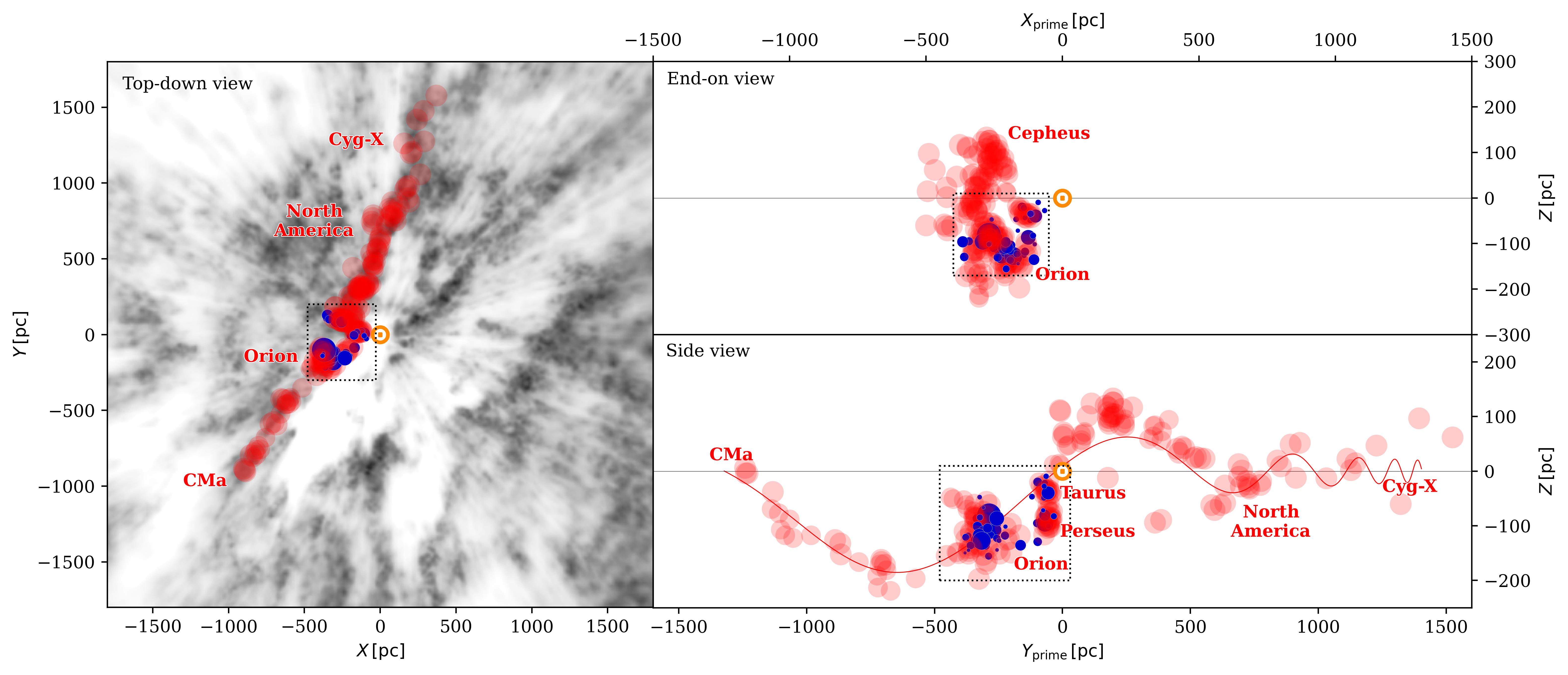
In this paper, we investigate the possible encounter between the Sun and the Radcliffe wave. The Radcliffe wave (Alves et al., 2020) is a narrow (aspect ratio of 1:20) and coherent 2.7-kpc-long sinusoidal gas structure, which comprises many known star-forming cloud complexes, such as CMa, Orion, Taurus, Perseus, Cepheus, North America nebula, and Cygnus. This gas structure, with an estimated mass of , appears to coherently oscillate like a traveling wave (Konietzka et al., 2024) and it is thought to be part of the Galaxy spiral structure (Swiggum et al., 2022). We used recent open cluster catalogs to identify a subset of young (), open clusters associated with the Radcliffe wave. By leveraging the new information regarding the 3D structure of the local ISM and the 3D spatial motions of the selected open clusters, used as tracers of the motion of the primordial clouds out of which they were born, we investigate potential interactions of our Solar System and the Radcliffe wave. Additionally, we discuss the possible geological signatures and climate effects that such an interaction could produce.
This paper is organized as follows. In Sect. 2, we outline the data used for the study. In Sect. 3, we describe the selection of the Radcliffe wave clusters, the estimation of their properties, such as age and mass, along with the properties of their parental clouds, and the method for orbit integration. We discuss the results and their interdisciplinary connections with other fields of study in Sect. 4 and we summarize our findings in Sect. 5.
2 Data
The Galactic cartesian coordinates () of the molecular clouds constituting the Radcliffe wave structure are taken from the studies by Zucker et al. (2019) and Alves et al. (2020). The molecular clouds catalog by Zucker et al. (2019) was constructed using a Bayesian statistical method, incorporating optical and near-infrared photometry, along with astrometric data, from the Pan-STARRS survey (Chambers et al., 2019; Flewelling et al., 2020), the 2MASS survey (Skrutskie et al., 2006), the NOAO source catalog (Nidever et al., 2018), and parallaxes from the second Gaia Data Release (Arenou et al., 2018; Gaia Collaboration et al., 2018). We used the positions of the clouds that constitute the Radcliffe wave to identify young clusters that may be associated with it.
For the clusters, we primarily used the recent open star cluster catalog by Hunt & Reffert (2023) (hereafter, HR23). This catalog was constructed by applying the Hierarchical Density-Based Spatial Clustering of Applications with Noise routine (McInnes et al., 2017) (HDBSCAN) on the Gaia DR3 astrometrical data (Gaia Collaboration et al., 2023) and the results were validated through a statistical density test and a Bayesian convolutional neural network. The catalog comprises a total of 7166 star clusters and provides a broad array of parameters. Of particular importance for our research are the sky positions, parallaxes, proper motions, radial velocities (RVs), estimated ages, extinctions, and stellar membership lists. To get better statistics for the full 6D phase space, we added additional RV data to the existing Gaia DR3 RVs. We cross-matched the stellar members of each cluster to the following surveys: APOGEE-2 SDSS DR17 (Abdurro’uf et al., 2022), GALAH DR3 (Buder et al., 2021), RAVE DR6 (Steinmetz et al., 2020), Gaia ESO DR6 (Randich et al., 2022), LAMOST DR5 (Zhao et al., 2012; Tsantaki et al., 2022), and two RV compilations (Gontcharov, 2006; Torres et al., 2006). In cases where a star is present in multiple surveys, we selected the RV value with the lowest uncertainty. Before recomputing the clusters’ median RVs, we first excluded stars with RV errors greater than and, secondly, we applied sigma-clipping using 3-sigma around the cluster median. To further ensure the accuracy of our results, we imposed a minimum requirement of at least five stars used in the computation of each cluster’s median RV and we considered only those clusters with RV errors below . Clusters that have only three or four stellar members with RVs were included again if the standard error is below , since these show a very narrow distribution in RV space. We then computed each cluster’s mean Galactic cartesian velocities () and the corresponding standard error (see Table 2). To ensure the positional accuracy of our results, we considered only those clusters with positional errors below 50 pc for the positions. Subsequently, we checked that none of the discarded clusters held relevance for our findings. Moreover, we compared our selection to the one used in a recent paper that investigated the Radcliffe wave’s motions (Konietzka et al., 2024). In that study, the authors used a compilation of several cluster catalogs (Sim et al., 2019; Liu & Pang, 2019; Cantat-Gaudin et al., 2020; Szilágyi et al., 2021; Hao et al., 2022; He et al., 2022) that predated HR23. We found that seven clusters of relevance to this study were missing from our selection. We computed the median positions and velocities of these additional clusters using the membership lists from the auxiliary cluster catalogs and cross-matches with the mentioned RV catalogs, deploying the same procedure as outlined above. As a result, four additional clusters passed our quality check: CWNU 1028, NGC 1977, OC 0340, and UBC 207. The Galactic positions and velocities of the clusters, reported in Table 2, were then used to integrate their orbits in the past. More information are provided in Sect. 3.
3 Methods
3.1 Identification of the Radcliffe wave’s clusters
We identified the clusters that could be associated with the Radcliffe wave by using the catalog of molecular clouds that constitute this structure (Alves et al., 2020) and the cluster sample described in Sect. 2. As a first step, we considered the clusters that, at the present day, are within 60 pc to the major molecular clouds and tenuous gas connections comprising the Radcliffe wave. We opted for this conservative threshold, as the radius of the Radcliffe wave has been estimated to be around 50 pc by Konietzka et al. (2024). Extending the threshold to 60 pc accounts for positional uncertainties that might bring clusters into this range. We chose not to include clusters farther away as their connection to the Radcliffe wave would be more uncertain. Additionally, we investigated the clusters that are located between 60 and 100 pc, and we verified that they are not relevant to our results. Using this distance criterion, we initially selected 104 clusters. As a second step, since we are interested in relatively young clusters whose motion may still be related to the gas phase of the Radcliffe wave, we applied an age cut and only considered those with an age estimate smaller than 30 Myr. We computed the ages of the clusters using the Gaia DR3 photometry, employing the procedure described in Sect. 3.2 and Appendix A.1. After applying the age cut, we were left with a total of 74 clusters that we consider to be associated with the Radcliffe wave. As a final selection step, we did a preliminary orbit integration over the past 30 Myr (for the integration details, see Sect. 3.4) to check which clusters come closer than 300 pc to the Sun in this time frame. This left us with a sample of 56 clusters.
In Fig. 1, we show the present-day positions of the 56 identified clusters, along with the molecular clouds comprising the Radcliffe wave. The heliocentric positions and velocities of the clusters are listed in Table 2. The selected clusters belong to the Taurus, Perseus, and Orion star-forming regions of the Radcliffe wave (see Table 3). The cluster names used in this work are listed in Table 3. We primarily use the names from the assembled cluster catalogs, while we have renamed some of the selected clusters with their previously defined and more widely recognized names, in cases where a significant cross-match of their stellar members aligns with those of previous studies (Chen et al., 2020a; Pavlidou et al., 2021; Krolikowski et al., 2021).
We used the 3D positions and velocities of the selected clusters to estimate their past orbits in the Milky Way as well as the previous orbits of the molecular clouds out of which they formed. The past positions of the gas clouds were inferred from the pre-birth trajectories of the clusters associated with them. This is based on the momentum conservation principle, which implies that the velocities of newly formed and young clusters are correlated with those of the center of mass of the natal gas (see e.g., Fernández et al., 2008; Tobin et al., 2009; Hacar et al., 2016; Großschedl et al., 2021; Konietzka et al., 2024). As the trajectories of these clusters appear to be interconnected rather than independent, exhibiting common motion (see also Sect. 4.1), and as they are all part of the Radcliffe wave, we interpret the orbits of their natal clouds as tracers of a larger gas complex. In this view, the gas clouds should not be considered as isolated objects but rather as parcels of a bigger gas structure. The fragmentation of this structure produced several bound, dense gas clumps where the analyzed star clusters subsequently formed. For simplicity, we adopt this decomposition into distinct “clouds” and refer to these parcels of gas as clouds throughout the paper. Notable examples within the analyzed region include the Orion A and Orion B giant molecular clouds, which extend for about 200 pc, each containing many embedded clusters. We acknowledge that this modeling approach simplifies the real structure and evolution of the gas clouds, but it is the only one applicable in this case since the exact shape of a cloud in the past cannot be recovered, as the gas is not rigid and its distribution is influenced by multiple mechanisms (see also Sect. 3.3). Considering these systematic uncertainties, the trajectories of the clusters and their parental clouds should be considered as preliminary estimates of the actual cloud paths. We refer the reader to Sects. 3.2, 3.3, and 3.4, for more details on the properties of the clusters, the properties of the parental clouds, and the orbit integration, respectively.
3.2 Estimation of ages and masses of the Radcliffe wave’s clusters
In this paper, we mainly used the HR23 cluster catalog, which already provides a homogeneous estimate of cluster ages and extinctions, using an approximate Bayesian neural network model which was trained on simulated data. However, as the age estimation was not the main focus of that paper, we recomputed the ages with a more robust and slightly more computationally expensive method. This method uses the recently developed Python package Chronos (see Ratzenböck et al., 2023b, for more details), which is capable of estimating the age, extinction, and metallicity of a cluster by performing a Bayesian fit of each cluster’s stellar members to theoretical model isochrones. We decided to use the PARSEC models (Bressan et al., 2012; Nguyen et al., 2022) in combination with Gaia DR3 photometry. We assumed the clusters to have the same metallicity, as they are young () and spatially close. We adopted a solar metallicity, since the chemical composition of Radcliffe wave clusters has been shown to be compatible with that of the Sun (see e.g., Alonso-Santiago et al., 2024). We also recomputed the ages for the clusters not present in HR23 (see Sect. 2 for more details). In Table 3, we report the estimated ages for the 56 clusters of the Radcliffe wave that we are considering in this work. In Fig. A.1 and A.2, we show the color-magnitude diagrams that are used for isochrone fitting. In Fig. A.3, we compare the ages of the clusters computed in this work with the ones provided by the source catalogs. We refer the reader to Appendix A.1 for more details.
We estimated the mass of a given cluster by summing the masses of its stellar members, which were determined from the isochrone fitted by Chronos. To correct for the incompleteness of the cluster’s members, possibly due to observational limits or stellar evolution, we compared the measured mass distributions to the initial mass function (IMF) by Kroupa (2001). By minimizing the total mass difference between a given IMF and the inferred one, we obtained the IMF that best fits our data. This minimization was performed within the mass range of 0.3 and , which is determined by the completeness limits of Gaia data (Meingast et al., 2021; Gaia Collaboration et al., 2023). The low-mass end limit of the Kroupa IMF was set to , to account for objects that are below the hydrogen-burning limit. We did not specify a high-mass bound to account for potentially missing massive sources that are either too bright for Gaia or have undergone SN explosion. In Table 3, we list the total masses of the clusters obtained by summing the masses of their members and those derived from the best-fit mass functions. In Fig. A.4, we show the best-fit mass functions, together with the inferred ones, for each of the clusters under analysis.
The reported cluster masses should be regarded as lower limits. This is due to various uncertainties, including the limitations of the HDBSCAN clustering algorithm. These limitations also subsequently affect the cloud radii and estimated number of SN (see Sect. 3.3 and Appendix A.3). The HDBSCAN algorithm indeed may not select all stellar members of each cluster, even if a star falls within a mass range where Gaia data is considered complete. This issue is inherent to all clustering algorithms, as they operate based on their own assumptions that may not fully encompass the wide range of cluster shapes, densities, and sizes. The presence of this systematic bias becomes evident when comparing different solutions from various clustering methods and attempts within the same region (see Ratzenböck et al., 2023a, for details).
3.3 Properties of the parental clouds associated with the clusters
For the times preceding the birth of a given cluster during the orbital tracebacks, we assumed the primordial clouds of the Radcliffe wave to have an onion-like structure. Each cloud was modeled as a set of concentric spheres with radii of 20, 30, 40, and 50 pc, representing the denser central parts and lower-density outskirts of each cloud. This modeling approach allows us to simplify the complex and varied structures exhibited by gas clouds. Indeed, molecular gas is typically organized into distinct, filamentary clouds (see e.g., André et al., 2010; Molinari et al., 2010; Li et al., 2013; Zucker et al., 2018; Imara & Forbes, 2023) arranged hierarchically, ranging from giant complexes spanning up to 100 pc, down to smaller, denser cores of few parsec in size (see e.g., Ferrière, 2001; Motte et al., 2018). These clouds can be surrounded by more diffuse gas (see e.g., Snow & McCall, 2006) and are constantly influenced by various physical mechanisms acting on different scales. These mechanisms include Galactic mechanisms (see e.g., Inutsuka et al., 2015), stellar feedback (see e.g., Walch & Naab, 2015; Großschedl et al., 2021; Posch et al., 2023), and magnetic fields (see e.g., Hennebelle & Inutsuka, 2019). Our approach is thus motivated by the fact that we cannot determine the past shapes of the clouds from the data.
In addition to the onion structure modeling, which aims to include the extension of both the tenuous gas and the central parts of the parental clouds associated with the clusters, we computed an estimate of the mass and radius of the densest part () of the gas clouds. We estimated the mass of the gas cloud associated with a given cluster () as
| (1) |
where is the stellar mass of the cluster corrected for incompleteness, as described in the Sect. 3.2, and SFE is the star formation efficiency for the Radcliffe wave, which is assumed to vary between 1% and 3% (see e.g., Kennicutt & Evans, 2012; Swiggum et al., 2022), though higher values have also been reported for the SFE in molecular clouds (see e.g., Chevance et al., 2020).
We used a mass-size relation to estimate the radius of an equivalent sphere with the same mass as our estimated cloud masses. Such relations have been studied both observationally and numerically, starting with the work of R.B. Larson (Larson, 1981), which was recently updated with the help of Gaia data, delivering a new 3D perspective for molecular clouds (see also Sect. 1). It has been found (Cahlon et al., 2024) that the masses of the clouds scale in relation to their volume () when 3D data are used, whereas they scale with the area () when the 3D data are projected onto a 2D plane. This is consistent with the predictions of previous theoretical and numerical studies (see e.g., Shetty et al., 2010; Beaumont et al., 2012; Ballesteros-Paredes et al., 2019). Therefore, we estimated the radius of the densest part for the parental clouds using the observationally based 3D mass-size relation from Cahlon et al. (2024),
| (2) |
We list the resulting cloud radii and masses in Table 3. By assuming a SFE of 1% (3%), the estimated masses of the clouds span from () for lambda-Ori to () for L1546. The corresponding estimated radii for these clouds are 30.7 pc (21.0 pc) and 5.0 pc (3.4 pc), respectively. As outlined in Sect. 3.2, the cloud radii and masses are likely underestimated and should be considered as lower limits, resulting from the incompleteness of stellar members in the cluster catalogs.
3.4 Orbit integration
We estimated the past orbits of the clusters, the associated clouds, and the Sun using the Galactic dynamics package galpy (Bovy, 2015) in combination with the Astropy package (Astropy Collaboration et al., 2022). galpy offers the possibility to numerically integrate orbits over different Milky Way potentials and initial conditions, such as the Galactocentric distance, the Sun’s height above the disk mid-plane, and the Sun’s velocity.
For our study, we used galpy’s MWPotential2014 as a model for the Milky Way’s gravitational potential. This model includes a bulge, a disk, and a halo component that are modeled as a power-law density profile with an exponential cut-off, a Miyamoto-Nagai potential, and a Navarro–Frenk–White profile, respectively (see Bovy, 2015, for details). We assumed a solar Galactocentric radius of (Gillessen et al., 2009) and a vertical position of (Chen et al., 2001). The Sun’s velocity relative to the Local Standard of Rest, whose circular velocity is set to the default galpy value of , is () = (11.1, 12.24, 7.25) (Schönrich et al., 2010). These parameters are internally used by galpy to change the reference frame from the Sun’s coordinate system to the Galactic center’s coordinate system before performing the orbit integration. The initial positions and velocities of the clusters, defined using the Astropy package, serve as input for galpy’s orbit module. Our integration covered the past 30 Myr, with a time-step of 0.03 Myr. We employed galpy’s dop853-c method, a Dormand-Prince integrator known for its reliability and speed.
We addressed the statistical uncertainties in the positions and velocities of the Sun and clusters by integrating their orbits 1000 times, each using new sets of data obtained by sampling the uncertainty distribution with a Monte Carlo sampling method. The initial positions and velocities of the considered clusters with respect to the Sun, along with the errors, are listed in Table 2, while the errors on the solar parameters are sourced from the provided references. Being aware of the fact that there is not a unique definition of the solar parameters and of the Milky Way potential, in Appendix B we tested the effect that different initial conditions have on our results. We conclude that the past trajectories of the Sun and the clusters, and their relative distances, do not significantly vary over the last 30 Myr when altering the described parameters. This can be attributed to the relatively short integration time considered, as found from prior studies (see e.g., Miret-Roig et al., 2020), and supports the robustness of our conclusions.
| Name | ||||||||
|---|---|---|---|---|---|---|---|---|
| Briceno 1 | - | - | - | - | ||||
| OBP-West | - | - | - | - | ||||
| OBP-d | - | - | - | - | ||||
| Sigma Orionis | - | - | - | - | - | - | ||
| NGC 1980 | ||||||||
| NGC 1981 | ||||||||
| NGC 1977 | - | - | - | - | ||||
| Radcliffe wave | ||||||||
4 Results and discussion
4.1 Solar System’s crossing of the Radcliffe wave
To assess a potential crossing of the Radcliffe wave by the Solar System, we computed, at each time step of the orbits tracebacks, the distances between the Sun and the clusters. For time intervals preceding the age of a given cluster, we considered its pre-birth trajectory as a first approximation of the orbit of the primordial cloud associated with it. As described in Sect. 3.1, we interpret the motion of the analyzed clouds as tracing the motion of the larger gas complex they belong to. By computing the time ranges in which the Sun and the center of the parental gas clouds are closer than their radii —considered as threshold distances— we were able to determine when the Sun most likely crossed these clouds and consequently the Radcliffe wave. We deemed a crossing significant if its probability of occurrence exceeds 50%. This was computed by repeating the tracebacks of the orbits multiple times, as described in Sect. 3.4.
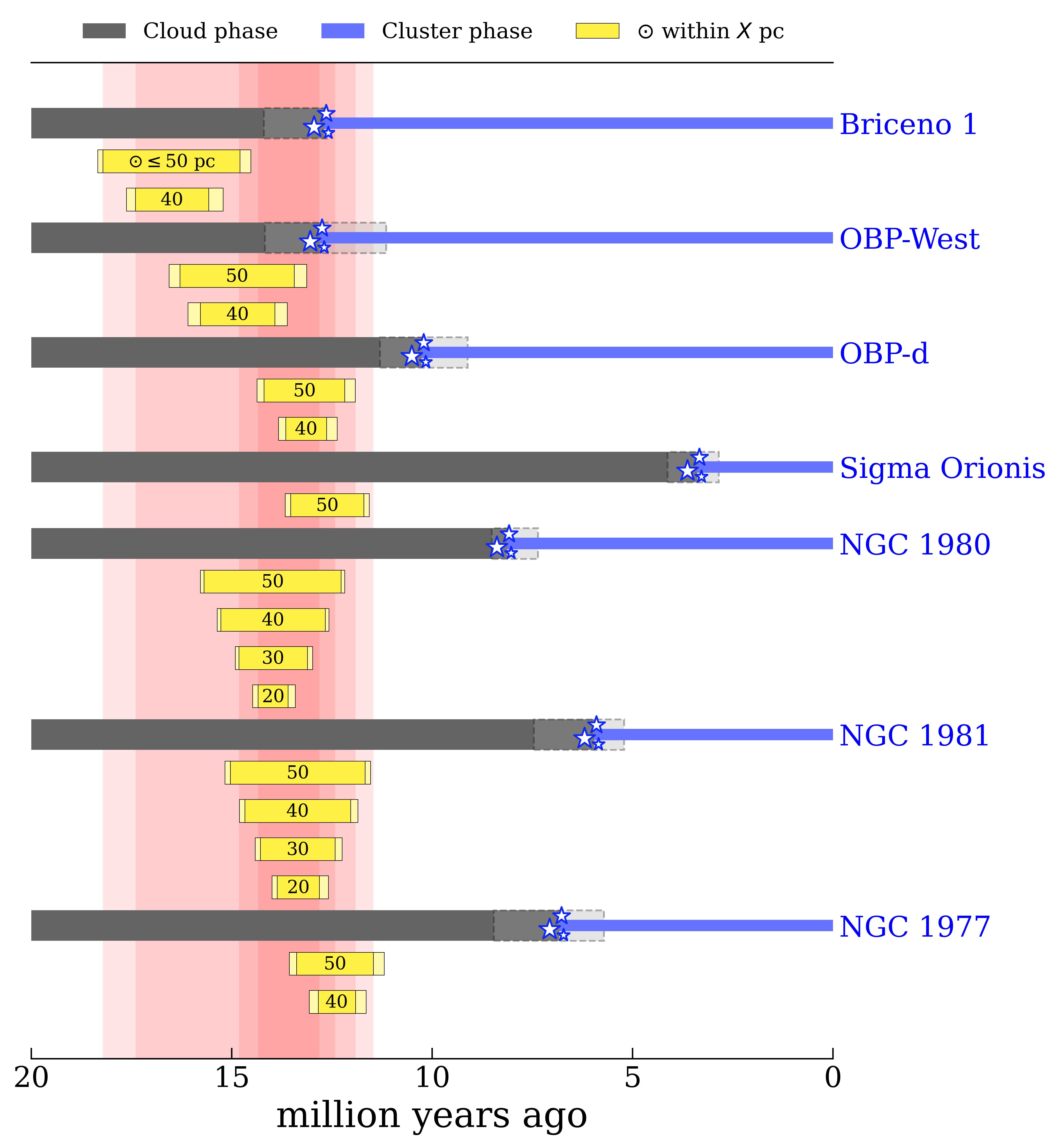
Remarkably, we find that the past trajectories of the Solar System closely approached ( within 50 pc) certain selected clusters while they were in their cloud phase, hinting at a probable encounter between the Sun and the gaseous component of the Radcliffe wave. When considering a cloud as a sphere of gas spanning 50 pc, we observe that the Sun’s orbit was concurrently passing through multiple parental clouds associated with the clusters Briceno 1, OBP-West, OBP-d, Sigma Orionis, NGC 1980, NGC 1981, and NGC 1977 between and Myr ago. These clusters are currently located within the Orion star-forming complex. It is relevant and interesting to note, from a historical perspective, that a possible crossing of the Orion region by the Solar System was already suggested by Shapley (1921), based on much less reliable data. Assuming a threshold distance of 40 pc, the Sun would still cross the gas clouds of all these clusters, with the exception of Sigma Orionis, approximately from to Myr ago. Considering 30 pc and 20 pc radii, the Solar System is within the parental clouds of NGC 1980 and NGC 1981 between and Myr ago, and and Myr ago, respectively. These time ranges are approximate since gravitational scattering from the clouds and stellar feedback are not accounted for; however, given the short integration times (less than 30 Myr; see e.g., Kamdar et al., 2021), the presented approximations are a valid first step to better understand the past Sun and clouds interactions.
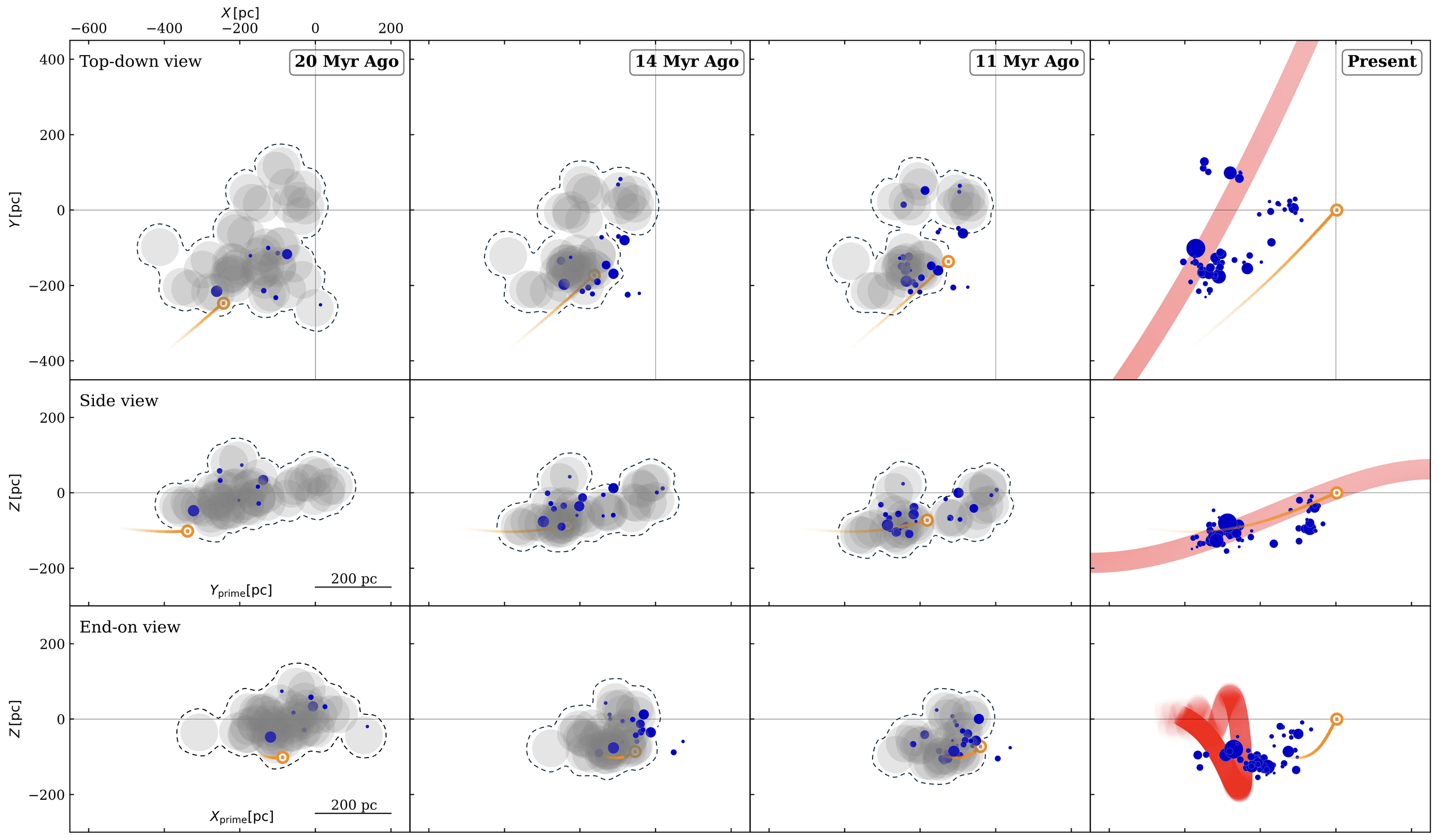
The crossing time ranges of the Radcliffe wave by the Sun are shown in Fig. 2 and listed in Table 1. A complete animation illustrating the orbital trajectories of the clusters, clouds, and Sun over the past 30 Myr is presented in Fig. 3 (interactive). In the static version, we depict four different snapshots at Myr, Myr, Myr, and the present. It can be seen that the Sun was approaching, crossing, and leaving the Radcliffe wave. In Fig. 3, we enclose the represented clouds with a dashed line, emphasizing the fact that they should be considered as part of a larger gas complex. From the interactive version of the figure, it is possible to note that the orbits of these clusters exhibit common motion. For some, their birthplaces likely indicate a shared formation history, although they do not need to come from exactly the same point in space. This is supported by the fact that some of the analyzed clusters belong to one of the three families of clusters identified in the work by Swiggum et al. (2024). For example, UPK 398, ASCC 18, ASCC 20, OCSN 64, OCSN 65, and CWNU 1072 are part of the Collinder 135 cluster family. Clusters in each of these three families converge toward each other when traced backward in time, consistent with shared formation origins (see Swiggum et al., 2024, Extended Data Fig. 1). Additionally, previous studies have already examined most of these clusters in the context of Orion (see e.g., Bally et al., 1987; Brown et al., 1994; Briceno, 2008; Alves & Bouy, 2012; Chen et al., 2020a; Kounkel, 2020; Großschedl et al., 2021).
For the seven clusters to which the Sun’s orbits get closer than 50 pc with a high probability, the estimated radii of the densest parts of the associated gas clouds (densities higher than 40 particles per ) range between 11.9–21.2 pc when considering 1% SFE, or 8.2–14.5 pc for a 3% SFE (refer to Sect. 3.3 and Table 3). Especially noteworthy is the case of NGC 1980, one of the two clusters to which the Solar System approaches within 20 pc. For this cluster, we estimated a radius of 21.2 pc (14.5 pc), which further supports our crossing hypothesis. It is important to clarify that the estimated radii pertain to the densest part of the clouds, which can then be surrounded by tenuous gas enveloping the central regions (see e.g., Snow & McCall, 2006). Moreover, these radii should be considered as lower limits, given the likely incompleteness of the cluster catalog, as previously highlighted in Sect. 3.3. We remark that these findings hold true even when assuming other initial conditions for the Sun’s parameters and different Milky Way potentials (see Appendix B for details).
4.2 Interdisciplinary bridges: Potential geological and climate evidences
The crossing of a dense region of the ISM by the Sun, such as a gas cloud or a SN blast wave, can impact the Solar System in various ways (see e.g., Fields & Wallner, 2023; Opher et al., 2024a). For example, the compression of the heliosphere by enhanced ram pressure exposes parts of the Solar System to the cold and dense ISM (see e.g., Miller & Fields, 2022; Opher et al., 2024a, b). The amount of dust loaded into Earth’s atmosphere would also increase, probably enhancing the delivery of radioisotopes (e.g., 60Fe) via dust grains (see e.g., Altobelli et al., 2005; Breitschwerdt et al., 2016). This could lead to anomalies in geological radionuclide records (Koll et al., 2019; Wallner et al., 2015, 2021) and could provide evidence of the passage of the Sun through the Radcliffe wave. Our estimates suggest that the Orion region traversed by the Sun may have been enriched with radioisotopes from SN before 11.5 Myr ago, with the potential incompleteness of the stellar membership in the catalogs increasing this estimate. For the estimation of the number of past SN events, we refer to Appendix A.3. Although current 60Fe data do not cover our period of interest (Fields & Wallner, 2023), future instrumentation is expected to be sensitive enough to analyze this time period.
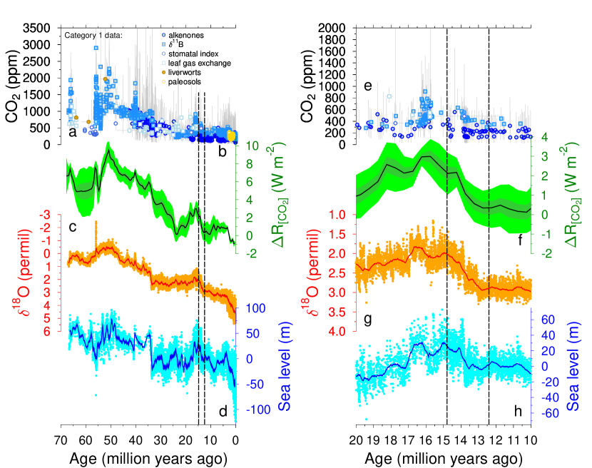
Furthermore, an increased amount of dust could impact Earth’s radiation budget, potentially leading to a cooling effect (see e.g., Talbot & Newman, 1977; Pavlov et al., 2005). Notably, our estimated time interval for the Solar System’s potential location within a dense ISM region (about Myr ago for a distance of pc from the center of a gas cloud) overlaps with the Middle Miocene climate transition (Steinthorsdottir et al., 2021). During this period, the expansion of the Antarctic ice sheet (Miller et al., 2020) and global cooling (Westerhold et al., 2020) marked Earth’s final transition to persistent large-scale continental glaciation in Antarctica (see Fig. 4, panel c-d and g-h). The ice sheet-climate interactions during the Miocene are complex (Knorr & Lohmann, 2014; Stap et al., 2024) and the evolving understanding suggests that this cooling phase was possibly caused by falling atmospheric concentrations (Cenozoic CO2 Proxy Integration Project Consortium(2023), CenCO2PIP) (Fig. 4, panel b and f). However, reconstructions beyond what is covered in Antarctic ice core data (the last 0.8 Myr) are highly uncertain (Fig. 4, panel a and e) and , when reconstructed from alkenones (van de Wal et al., 2011) (Fig. 4, panel e, light blue circles), seem indeed to suggest that the Middle Miocene cooling was not directly coupled to radiative forcing. Therefore, it is intriguing to consider that the passage of our Solar System through a dense region of the ISM might have contributed to this climate transition, even if this remains speculative and currently lacks direct proof. We cautiously point out such possibilities to make the community aware of maybe overlooked processes, but we are conscious that available 60Fe data do not extend beyond 10 Myr ago (Fields & Wallner, 2023) and to our knowledge no rise in dust load has yet been discovered around 14 Myr ago in deep sea sediments (Rea, 1994). Furthermore, the suggested decoupling of Middle Miocene temperature and alkenone-based , that opens up the possibility that not but other processes are responsible for the reconstructed cooling, needs to be taken with caution, since recently various authors have suggested that some fundamental difficulties exist in studies that used alkenones for the reconstruction of atmospheric (e.g., Phelps et al., 2021; Rae et al., 2021; Brandenburg et al., 2022).
We compared the radiative forcing and climate response during the Middle Miocene cooling period to what is known for the ice ages of the Pleistocene ( Myr ago), in order to estimate by how much the extraterrestrial dust flux to Earth needs to have changed during the Solar System’s crossing of the Radcliffe wave to serve as the primary driver of this climate transition - alternatively to atmospheric concentrations. We based our analysis on the Pleistocene, as this period has a significantly more extensive data coverage. However, we acknowledge that this is an imperfect comparison, partly due to differences in the time scales of climate change (Myr in the Middle Miocene versus kyr in the Pleistocene), and because the radiative forcing changes during the Middle Miocene climate transition and late Pleistocene ice ages are of similar size, yet linked to different climate responses. Nonetheless, we used this comparison to obtain an order of magnitude estimate of the required change in dust flux.
During the Middle Miocene climate transition, the long-term mean radiative forcing of shows a reduction by (Fig. 4, panel f). Concurrently, the long-term and global mean surface temperature, estimated from benthic (Fig. 4, panel g), decreased by more than (Westerhold et al., 2020) and sea level dropped by (Fig. 4, panel h). We refer to Rohling et al. (2024) for the ongoing discussion on apparent discrepancies in reconstructed Cenozoic climate change based on different proxies. During glacial periods of the late Pleistocene, a similar reduction in radiative forcing, together with other forcing and feedback processes (Köhler et al., 2010), led to a global mean surface cooling of approximately (Tierney et al., 2020; Clark et al., 2024) and to land ice sheets growth, mainly in North America and Eurasia. This ice sheets expansion corresponded to a sea level drop of about (Gowan et al., 2021). The root cause of Pleistocene glaciations is understood to be the changes of Earth’s orbital parameters (Milankovic, 1941; Barker et al., 2024), which led to variations in incoming solar radiation (Laskar et al., 2004). Nevertheless, reduced greenhouse gas concentrations, increased atmospheric dust load, and higher surface albedo are important contributions necessary to drive Earth’s climate into an ice age (Köhler et al., 2010).
During the late Pleistocene ice ages, the glacial dust (i.e., global dust during ice ages) deposition rate was times larger than today (Albani et al., 2016; Mahowald et al., 2023) and, although the impact of dust on the climate is complex (Kok et al., 2023) and with significant uncertainties (Mahowald et al., 2023), it contributed to a radiative forcing of about (Köhler et al., 2010; Shaffer & Lambert, 2018; Sherwood et al., 2020), roughly half of the change in radiative forcing caused by atmospheric . Given that the present-day global dust deposition rate on Earth is (Kok et al., 2021), it would need to rise to in order achieve a radiative forcing similar to that proposed so far for during the Middle Miocene climate transition. Furthermore, the current incoming flux of extraterrestrial dust load is on top of the atmosphere, which decreases to at the surface (Love & Brownlee, 1993; Plane, 2012; Rojas et al., 2021). Therefore, for the crossing of the Radcliffe wave to be the main driver of the Middle Miocene cooling, the extraterrestrial dust flux would need to rise by about orders of magnitude to produce such a large anomaly in the radiation budget and the resulting climate effects. At present, the Sun is located at the edge of the Local Interstellar Cloud (LIC), a low-density cloudlet with (see e.g., Gry & Jenkins, 2014), located within a SN-generated hot void known as the Local Bubble, which has a characteristic density of (see e.g., Cox & Reynolds, 1987; Linsky & Redfield, 2021; Zucker et al., 2022; O’Neill et al., 2024). As the ISM density of the Radcliffe wave is significantly higher (ranging from to ) than the region currently traversed by the Solar System, the increase in the dust load on Earth could be at least of orders of magnitude. Consequently, considering all factors and disregarding other differences in the climate system between the late Pleistocene and the Middle Miocene, our study suggests that the potential rise in extraterrestrial dust during the Solar System’s crossing of the Radcliffe wave may have been orders of magnitude smaller than necessary to fully account for the Middle Miocene climate transition as observed in the geological record. At the moment, we can therefore infer that this process likely played a limited role in the Middle Miocene climate transition. However, once some of the underlying assumptions of this estimate are better constrained, the contribution to this event might be reassessed in either direction. Additionally, due to the nonpermanent nature of any extraterrestrial dust influx associated with the Solar System’s crossing, this process alone is unlikely to account for the long-term effect of a reduction in atmospheric . While it may have influenced climate during the multi-million years duration of the passage, other forcings or feedbacks would be required to explain the persistence of low temperatures and sea levels following the Middle Miocene climate transition.
To conclude, present day knowledge suggests that beyond small solar-driven climate oscillations (Eddy, 1976), the long-term energy output of the Sun (Gough, 1981) together with Earth’s orbital parameters (Milankovic, 1941), plate tectonics (Scotese, 2021), deep carbon cycle (Müller et al., 2022), internal feedback (Ganopolski, 2024), and very few large-scale meteorite impacts (Osinski et al., 2022; Zorzi et al., 2022) can explain a wide spectrum of the reconstructed changes and variability in Cenozoic climate. So far, all proposed additional extra-terrestrial influences have, to our knowledge, remained in a hypothetical state (Pavlov et al., 2005; Opher et al., 2024a) or even been discarded (Berger, 1999; Carslaw et al., 2002; Bard & Frank, 2006). However, we cannot rule out the possibility that an extraordinary amount of dust in the entire inner Solar System might have led to a reduction of incoming Solar radiation and a cooling on Earth, similar to what has been proposed for the triggering of the mid-Ordovician ice age 466 My ago (Schmitz et al., 2019). Furthermore, as shown by Miller et al. (2024), some effects of the Solar System’s passage through a dense ISM region may be linked to nonpermanent, seasonal variations in cloud formation on Earth, which are more difficult to detect in paleo-records.
4.3 Caveats
Our results are based on the tracebacks of the orbits of the Solar System and of the clusters associated with the Radcliffe wave. As noted throughout the text, this method requires some approximations due to inherent difficulties in modeling the past structure and evolution of the gas. For example, we simplified the diverse and complex morphologies of the molecular clouds by assuming a spherical shape. Based on the principle of momentum conservation, we assumed that the motion of young clusters still reflects the movement of the gas nurseries from which they formed. We acknowledge that gravitational interactions and feedback from massive stars have likely influenced parts of the gas clouds and, consequently, the velocities of the clusters which formed within them. Thus, our tracebacks should be considered as a first approximation of the actual orbits. With these assumptions, we showed the general patterns of motion and estimate a time window during which the Solar System may have crossed the Radcliffe wave. Future studies will need to examine in greater detail the possible effects of gravity and feedback-induced displacements.
5 Conclusions
Our investigation reveals that the Solar System likely passed through the Orion region of the Radcliffe wave gas structure. By tracing back the orbits of the Sun and the Radcliffe wave’s clusters, we constrain the time range of this crossing to be between and Myr ago, with the closest approaches ( within pc) occurring within the interval of to Myr ago. As we do not account for potential gravitational interactions and feedback forces, we consider these time ranges to be preliminary approximations. Our results remain consistent even when varying solar parameters and Milky Way gravitational potentials.
The potentially increased amount of dust in the inner Solar System and in Earth’s atmosphere resulting from such an interaction provides a framework for searching for isotopic anomalies in geological records older than 10 Myr. This is supported by our estimate that approximately SN occurred in the region traversed by the Sun, thus seeding it with freshly produced isotopes, such as 60Fe. Additionally, we find that the period of closest approach was synchronous with the reorganization of the Earth’s climate known as the Middle Miocene climate transition, even though a causal connection between the two events remains speculative and lacks direct evidence. In conclusion, our investigations underline the importance of studying the Galactic environment encountered by the Solar System during its orbit, along with the potential effects this may have on Earth.
Data availability
The supplementary figures of the Appendix are available online via Zenodo at the following link: https://doi.org/10.5281/zenodo.14626660. The code used for the analysis will be shared by EM upon reasonable request.
Acknowledgements.
We thank the anonymous referee for the insightful comments, which have improved the quality and readability of the paper. JA and EM were co-funded by the European Union (ERC, ISM-FLOW, 101055318). S.R. acknowledges funding by the Austrian Research Promotion Agency (FFG, https://www.ffg.at/) under project number FO999892674. JG gratefully acknowledges co-funding from the European Union, the Central Bohemian Region, and the Czech Academy of Sciences, as part of the MERIT fellowship (MSCA-COFUND Horizon Europe, Grant Agreement No. 101081195). JG acknowledges the Collaborative Research Center 1601 (SFB 1601) funded by the Deutsche Forschungsgemeinschaft (DFG, German Research Foundation) – 500700252. This work has made use of data from the European Space Agency (ESA) mission Gaia https://www.cosmos.esa.int/gaia, processed by the Gaia Data Processing and Analysis Consortium (DPAC, https://www.cosmos.esa.int/web/gaia/dpac/consortium). Funding for the DPAC has been provided by national institutions, in particular the institutions participating in the Gaia Multilateral Agreement. This research has made use of publicly available software libraries, including galpy (Bovy, 2015), Astropy (Astropy Collaboration et al., 2022), NumPy (Harris et al., 2020), ALADIN (Bonnarel et al., 2000), TOPCAT (Taylor, 2011), matplotlib (Hunter, 2007), and plotly. The IMF has been sampled using the python code available at the following repository on github: https://github.com/keflavich/imf. The ages of the clusters have been estimated using the Chronos python code available at the following repository on github: https://github.com/ratzenboe/Chronos.References
- Abdurro’uf et al. (2022) Abdurro’uf, Accetta, K., Aerts, C., et al. 2022, ApJS, 259, 35
- Albani et al. (2016) Albani, S., Mahowald, N. M., Murphy, L. N., et al. 2016, Geochim. Res. Lett., 43, 3944
- Almeida et al. (2023) Almeida, A., Monteiro, H., & Dias, W. S. 2023, MNRAS, 525, 2315
- Alonso-Santiago et al. (2024) Alonso-Santiago, J., Frasca, A., Bragaglia, A., et al. 2024, arXiv e-prints, arXiv:2410.14373
- Altobelli et al. (2005) Altobelli, N., Kempf, S., Krüger, H., et al. 2005, Journal of Geophysical Research (Space Physics), 110, A07102
- Alves & Bouy (2012) Alves, J. & Bouy, H. 2012, A&A, 547, A97
- Alves et al. (2020) Alves, J., Zucker, C., Goodman, A. A., et al. 2020, Nature, 578, 237
- André et al. (2010) André, P., Men’shchikov, A., Bontemps, S., et al. 2010, A&A, 518, L102
- Arenou et al. (2018) Arenou, F., Luri, X., Babusiaux, C., et al. 2018, A&A, 616, A17
- Astropy Collaboration et al. (2022) Astropy Collaboration, Price-Whelan, A. M., Lim, P. L., et al. 2022, ApJ, 935, 167
- Ballesteros-Paredes et al. (2019) Ballesteros-Paredes, J., Román-Zúñiga, C., Salomé, Q., Zamora-Avilés, M., & Jiménez-Donaire, M. J. 2019, MNRAS, 490, 2648
- Bally et al. (1987) Bally, J., Langer, W. D., Stark, A. A., & Wilson, R. W. 1987, ApJ, 312, L45
- Bard & Frank (2006) Bard, E. & Frank, M. 2006, Earth and Planetary Science Letters, 248, 1
- Barker et al. (2024) Barker, S., Lisiecki, L., Knorr, G., Nuber, S., & Tzedakis, P. 2024, Science - under revision
- Beaumont et al. (2012) Beaumont, C. N., Goodman, A. A., Alves, J. F., et al. 2012, MNRAS, 423, 2579
- Bennett & Bovy (2019) Bennett, M. & Bovy, J. 2019, MNRAS, 482, 1417
- Berger (1999) Berger, W. H. 1999, International Journal of Earth Sciences, 88, 305
- Bonnarel et al. (2000) Bonnarel, F., Fernique, P., Bienaymé, O., et al. 2000, A&AS, 143, 33
- Bovy (2015) Bovy, J. 2015, ApJS, 216, 29
- Brandenburg et al. (2022) Brandenburg, K. M., Rost, B., de Waal, D. B. V., Hoins, M., & Sluijs, A. 2022, Biogeosciences, 19, 3305
- Breitschwerdt et al. (2016) Breitschwerdt, D., Feige, J., Schulreich, M. M., et al. 2016, Nature, 532, 73
- Bressan et al. (2012) Bressan, A., Marigo, P., Girardi, L., et al. 2012, MNRAS, 427, 127
- Briceno (2008) Briceno, C. 2008, in Handbook of Star Forming Regions, Volume I, ed. B. Reipurth, Vol. 4, 838
- Brown et al. (1994) Brown, A. G. A., de Geus, E. J., & de Zeeuw, P. T. 1994, A&A, 289, 101
- Buder et al. (2021) Buder, S., Sharma, S., Kos, J., et al. 2021, MNRAS, 506, 150
- Cahlon et al. (2024) Cahlon, S., Zucker, C., Goodman, A., Lada, C., & Alves, J. 2024, ApJ, 961, 153
- Cantat-Gaudin et al. (2020) Cantat-Gaudin, T., Anders, F., Castro-Ginard, A., et al. 2020, A&A, 640, A1
- Carslaw et al. (2002) Carslaw, K. S., Harrison, R. G., & Kirkby, J. 2002, Science, 298, 1732
- Cenozoic CO2 Proxy Integration Project Consortium(2023) (CenCO2PIP) Cenozoic CO2 Proxy Integration Project (CenCO2PIP) Consortium. 2023, Science, 382, eadi5177
- Chambers et al. (2019) Chambers, K. C., Magnier, E. A., Metcalfe, N., et al. 2019, arXiv e-prints, arXiv:1612.05560
- Chen et al. (2020a) Chen, B., D’Onghia, E., Alves, J., & Adamo, A. 2020a, A&A, 643, A114
- Chen et al. (2001) Chen, B., Stoughton, C., Smith, J. A., et al. 2001, ApJ, 553, 184
- Chen et al. (2020b) Chen, B. Q., Li, G. X., Yuan, H. B., et al. 2020b, MNRAS, 493, 351
- Chevance et al. (2020) Chevance, M., Kruijssen, J. M. D., Vazquez-Semadeni, E., et al. 2020, Space Sci. Rev., 216, 50
- Clark et al. (2024) Clark, P. U., Shakun, J. D., Rosenthal, Y., Köhler, P., & Bartlein, P. J. 2024, Science, 383, 884
- Cox & Reynolds (1987) Cox, D. P. & Reynolds, R. J. 1987, ARA&A, 25, 303
- Dehnen & Binney (1998) Dehnen, W. & Binney, J. J. 1998, MNRAS, 298, 387
- Dharmawardena et al. (2023) Dharmawardena, T. E., Bailer-Jones, C. A. L., Fouesneau, M., et al. 2023, MNRAS, 519, 228
- Eddy (1976) Eddy, J. A. 1976, Science, 192, 1189
- Edenhofer et al. (2024) Edenhofer, G., Zucker, C., Frank, P., et al. 2024, A&A, 685, A82
- Eisenhauer et al. (2003) Eisenhauer, F., Schödel, R., Genzel, R., et al. 2003, ApJ, 597, L121
- Fernández et al. (2008) Fernández, D., Figueras, F., & Torra, J. 2008, A&A, 480, 735
- Ferrière (2001) Ferrière, K. M. 2001, Reviews of Modern Physics, 73, 1031
- Fields & Wallner (2023) Fields, B. D. & Wallner, A. 2023, Annual Review of Nuclear and Particle Science, 73, 365
- Flewelling et al. (2020) Flewelling, H. A., Magnier, E. A., Chambers, K. C., et al. 2020, ApJS, 251, 7
- Foley et al. (2023) Foley, M. M., Goodman, A., Zucker, C., et al. 2023, ApJ, 947, 66
- Francis & Anderson (2014) Francis, C. & Anderson, E. 2014, MNRAS, 441, 1105
- Gaia Collaboration et al. (2018) Gaia Collaboration, Brown, A. G. A., Vallenari, A., et al. 2018, A&A, 616, A1
- Gaia Collaboration et al. (2016) Gaia Collaboration, Prusti, T., de Bruijne, J. H. J., et al. 2016, A&A, 595, A1
- Gaia Collaboration et al. (2023) Gaia Collaboration, Vallenari, A., Brown, A. G. A., et al. 2023, A&A, 674, A1
- Ganopolski (2024) Ganopolski, A. 2024, Climate of the Past, 20, 151
- Gillessen et al. (2009) Gillessen, S., Eisenhauer, F., Trippe, S., et al. 2009, ApJ, 692, 1075
- Gontcharov (2006) Gontcharov, G. A. 2006, Astronomical and Astrophysical Transactions, 25, 145
- Gough (1981) Gough, D. O. 1981, Sol. Phys., 74, 21
- Gould (1874) Gould, B. A. 1874, American Journal of Science and Arts, 8, 325
- Gowan et al. (2021) Gowan, E. J., Zhang, X., Khosravi, S., et al. 2021, Nature Communications, 12, 1199
- GRAVITY Collaboration et al. (2018) GRAVITY Collaboration, Abuter, R., Amorim, A., et al. 2018, A&A, 615, L15
- Green et al. (2019) Green, G. M., Schlafly, E., Zucker, C., Speagle, J. S., & Finkbeiner, D. 2019, ApJ, 887, 93
- Großschedl et al. (2021) Großschedl, J. E., Alves, J., Meingast, S., & Herbst-Kiss, G. 2021, A&A, 647, A91
- Gry & Jenkins (2014) Gry, C. & Jenkins, E. B. 2014, A&A, 567, A58
- Hacar et al. (2016) Hacar, A., Alves, J., Forbrich, J., et al. 2016, A&A, 589, A80
- Hao et al. (2022) Hao, C. J., Xu, Y., Wu, Z. Y., et al. 2022, A&A, 660, A4
- Harris et al. (2020) Harris, C. R., Millman, K. J., van der Walt, S. J., et al. 2020, Nature, 585, 357
- He et al. (2022) He, Z., Wang, K., Luo, Y., et al. 2022, ApJS, 262, 7
- Hennebelle & Inutsuka (2019) Hennebelle, P. & Inutsuka, S.-i. 2019, Frontiers in Astronomy and Space Sciences, 6, 5
- Hogg et al. (2005) Hogg, D. W., Blanton, M. R., Roweis, S. T., & Johnston, K. V. 2005, ApJ, 629, 268
- Hunt & Reffert (2023) Hunt, E. L. & Reffert, S. 2023, A&A, 673, A114
- Hunter (2007) Hunter, J. D. 2007, Computing in Science and Engineering, 9, 90
- Imara & Forbes (2023) Imara, N. & Forbes, J. C. 2023, ApJ, 956, 114
- Inutsuka et al. (2015) Inutsuka, S.-i., Inoue, T., Iwasaki, K., & Hosokawa, T. 2015, A&A, 580, A49
- Irrgang et al. (2013) Irrgang, A., Wilcox, B., Tucker, E., & Schiefelbein, L. 2013, A&A, 549, A137
- Kamdar et al. (2021) Kamdar, H., Conroy, C., & Ting, Y.-S. 2021, arXiv e-prints, arXiv:2106.02050
- Kennicutt & Evans (2012) Kennicutt, R. C. & Evans, N. J. 2012, ARA&A, 50, 531
- Kerr & Lynden-Bell (1986) Kerr, F. J. & Lynden-Bell, D. 1986, MNRAS, 221, 1023
- Knorr & Lohmann (2014) Knorr, G. & Lohmann, G. 2014, Nature Geoscience, 7, 376
- Köhler et al. (2010) Köhler, P., Bintanja, R., Fischer, H., et al. 2010, Quaternary Science Reviews, 29, 129
- Kok et al. (2021) Kok, J. F., Adebiyi, A. A., Albani, S., et al. 2021, Atmospheric Chemistry & Physics, 21, 8127
- Kok et al. (2023) Kok, J. F., Storelvmo, T., Karydis, V. A., et al. 2023, Nature Reviews Earth and Environment, 4, 71
- Koll et al. (2019) Koll, D., Korschinek, G., Faestermann, T., et al. 2019, Phys. Rev. Lett., 123, 072701
- Konietzka et al. (2024) Konietzka, R., Goodman, A. A., Zucker, C., et al. 2024, Nature, 628, 62
- Kos et al. (2019) Kos, J., Bland-Hawthorn, J., Asplund, M., et al. 2019, A&A, 631, A166
- Kounkel (2020) Kounkel, M. 2020, ApJ, 902, 122
- Krolikowski et al. (2021) Krolikowski, D. M., Kraus, A. L., & Rizzuto, A. C. 2021, AJ, 162, 110
- Kroupa (2001) Kroupa, P. 2001, MNRAS, 322, 231
- Lallement et al. (2019) Lallement, R., Babusiaux, C., Vergely, J. L., et al. 2019, A&A, 625, A135
- Lallement et al. (2022) Lallement, R., Vergely, J. L., Babusiaux, C., & Cox, N. L. J. 2022, A&A, 661, A147
- Larson (1981) Larson, R. B. 1981, MNRAS, 194, 809
- Laskar et al. (2004) Laskar, J., Robutel, P., Joutel, F., et al. 2004, A&A, 428, 261
- Leike et al. (2020) Leike, R. H., Glatzle, M., & Enßlin, T. A. 2020, A&A, 639, A138
- Li et al. (2013) Li, G.-X., Wyrowski, F., Menten, K., & Belloche, A. 2013, A&A, 559, A34
- Linsky & Redfield (2021) Linsky, J. L. & Redfield, S. 2021, ApJ, 920, 75
- Liu & Pang (2019) Liu, L. & Pang, X. 2019, ApJS, 245, 32
- Love & Brownlee (1993) Love, S. G. & Brownlee, D. E. 1993, Science, 262, 550
- Luo et al. (2015) Luo, A. L., Zhao, Y.-H., Zhao, G., et al. 2015, Research in Astronomy and Astrophysics, 15, 1095
- Mahowald et al. (2023) Mahowald, N. M., Li, L., Albani, S., Hamilton, D. S., & Kok, J. F. 2023, in AGU Fall Meeting Abstracts, Vol. 2023, A32C–01
- Majewski et al. (2017) Majewski, S. R., Schiavon, R. P., Frinchaboy, P. M., et al. 2017, AJ, 154, 94
- McInnes et al. (2017) McInnes, L., Healy, J., & Astels, S. 2017, The Journal of Open Source Software, 2, 205
- McMillan (2017) McMillan, P. J. 2017, MNRAS, 465, 76
- Meingast et al. (2021) Meingast, S., Alves, J., & Rottensteiner, A. 2021, A&A, 645, A84
- Milankovic (1941) Milankovic, M. 1941, Kanon der Erdbestrahlung und seine Anwendung auf das Eiszeitenproblem, 1st edn. (Belgrade: Mihaila Curcica)
- Miller & Fields (2022) Miller, J. A. & Fields, B. D. 2022, ApJ, 934, 32
- Miller et al. (2024) Miller, J. A., Opher, M., Hatzaki, M., Papachristopoulou, K., & Thomas, B. C. 2024, Geochim. Res. Lett., 51, e2024GL110174
- Miller et al. (2020) Miller, K. G., Browning, J. V., Schmelz, W. J., et al. 2020, Science Advances, 6, eaaz1346
- Miret-Roig et al. (2020) Miret-Roig, N., Galli, P. A. B., Brandner, W., et al. 2020, A&A, 642, A179
- Molinari et al. (2010) Molinari, S., Swinyard, B., Bally, J., et al. 2010, A&A, 518, L100
- Motte et al. (2018) Motte, F., Bontemps, S., & Louvet, F. 2018, ARA&A, 56, 41
- Müller et al. (2022) Müller, R. D., Mather, B., Dutkiewicz, A., et al. 2022, Nature, 605, 629
- Nguyen et al. (2022) Nguyen, C. T., Costa, G., Girardi, L., et al. 2022, A&A, 665, A126
- Nidever et al. (2018) Nidever, D. L., Dey, A., Olsen, K., et al. 2018, AJ, 156, 131
- O’Neill et al. (2024) O’Neill, T. J., Zucker, C., Goodman, A. A., & Edenhofer, G. 2024, arXiv e-prints, arXiv:2403.04961
- Opher et al. (2024a) Opher, M., Loeb, A., & Peek, J. E. G. 2024a, Nature Astronomy
- Opher et al. (2024b) Opher, M., Loeb, A., Zucker, C., et al. 2024b, ApJ, 972, 201
- Osinski et al. (2022) Osinski, G. R., Grieve, R. A., Ferrière, L., et al. 2022, Earth-Science Reviews, 232, 104112
- Pavlidou et al. (2021) Pavlidou, T., Scholz, A., & Teixeira, P. S. 2021, MNRAS, 503, 3232
- Pavlov et al. (2005) Pavlov, A. A., Toon, O. B., Pavlov, A. K., Bally, J., & Pollard, D. 2005, Geochim. Res. Lett., 32, L03705
- Phelps et al. (2021) Phelps, S. R., Stoll, H. M., Bolton, C. T., Beaufort, L., & Polissar, P. J. 2021, Geochemistry, Geophysics, Geosystems, 22, e2021GC009658
- Plane (2012) Plane, J. M. C. 2012, Chemical Society Reviews, 41, 6507
- Posch et al. (2023) Posch, L., Miret-Roig, N., Alves, J., et al. 2023, A&A, 679, L10
- Rae et al. (2021) Rae, J. W. B., Zhang, Y. G., Liu, X., et al. 2021, Annual Review of Earth and Planetary Sciences, 49
- Randich et al. (2022) Randich, S., Gilmore, G., Magrini, L., et al. 2022, A&A, 666, A121
- Ratzenböck et al. (2023b) Ratzenböck, S., Großschedl, J. E., Alves, J., et al. 2023b, A&A, 678, A71
- Ratzenböck et al. (2023a) Ratzenböck, S., Großschedl, J. E., Möller, T., et al. 2023a, A&A, 677, A59
- Rea (1994) Rea, D. K. 1994, Reviews of Geophysics, 32, 159
- Rohling et al. (2024) Rohling, E. J., Gernon, T. M., Heslop, D., et al. 2024, Paleoceanography and Paleoclimatology, 39, e2024PA004872
- Rojas et al. (2021) Rojas, J., Duprat, J., Engrand, C., et al. 2021, Earth and Planetary Science Letters, 560, 116794
- Schmitz et al. (2019) Schmitz, B., Farley, K. A., Goderis, S., et al. 2019, Science Advances, 5, eaax4184
- Schönrich et al. (2010) Schönrich, R., Binney, J., & Dehnen, W. 2010, MNRAS, 403, 1829
- Schulreich et al. (2017) Schulreich, M. M., Breitschwerdt, D., Feige, J., & Dettbarn, C. 2017, A&A, 604, A81
- Schulreich et al. (2023) Schulreich, M. M., Feige, J., & Breitschwerdt, D. 2023, A&A, 680, A39
- Scotese (2021) Scotese, C. R. 2021, Annual Review of Earth and Planetary Sciences, 49
- Shaffer & Lambert (2018) Shaffer, G. & Lambert, F. 2018, Proceedings of the National Academy of Science, 115, 2026
- Shapley (1921) Shapley, H. 1921, Journal of Geology, 29, 502
- Sherwood et al. (2020) Sherwood, S. C., Webb, M. J., Annan, J. D., et al. 2020, Reviews of Geophysics, 58, e2019RG000678
- Shetty et al. (2010) Shetty, R., Collins, D. C., Kauffmann, J., et al. 2010, ApJ, 712, 1049
- Sim et al. (2019) Sim, G., Lee, S. H., Ann, H. B., & Kim, S. 2019, Journal of Korean Astronomical Society, 52, 145
- Skrutskie et al. (2006) Skrutskie, M. F., Cutri, R. M., Stiening, R., et al. 2006, AJ, 131, 1163
- Snow & McCall (2006) Snow, T. P. & McCall, B. J. 2006, ARA&A, 44, 367
- Stap et al. (2024) Stap, L. B., Berends, C. J., & van de Wal, R. S. W. 2024, Climate of the Past, 20, 257
- Steinmetz et al. (2020) Steinmetz, M., Matijevič, G., Enke, H., et al. 2020, AJ, 160, 82
- Steinthorsdottir et al. (2021) Steinthorsdottir, M., Coxall, H. K., de Boer, A. M., et al. 2021, Paleoceanography and Paleoclimatology, 36, e2020PA004037
- Swiggum et al. (2024) Swiggum, C., Alves, J., Benjamin, R., et al. 2024, Nature, 631, 49
- Swiggum et al. (2022) Swiggum, C., Alves, J., D’Onghia, E., et al. 2022, A&A, 664, L13
- Szilágyi et al. (2021) Szilágyi, M., Kun, M., & Ábrahám, P. 2021, MNRAS, 505, 5164
- Talbot & Newman (1977) Talbot, R. J., J. & Newman, M. J. 1977, ApJS, 34, 295
- Taylor (2011) Taylor, M. 2011, TOPCAT: Tool for OPerations on Catalogues And Tables, Astrophysics Source Code Library, record ascl:1101.010
- Tierney et al. (2020) Tierney, J. E., Zhu, J., King, J., et al. 2020, Nature, 584, 569
- Tobin et al. (2009) Tobin, J. J., Hartmann, L., Furesz, G., Mateo, M., & Megeath, S. T. 2009, ApJ, 697, 1103
- Torres et al. (2006) Torres, C. A. O., Quast, G. R., da Silva, L., et al. 2006, A&A, 460, 695
- Tsantaki et al. (2022) Tsantaki, M., Pancino, E., Marrese, P., et al. 2022, A&A, 659, A95
- van de Wal et al. (2011) van de Wal, R. S. W., de Boer, B., Lourens, L. J., Köhler, P., & Bintanja, R. 2011, Climate of the Past, 7, 1459
- Vanhollebeke et al. (2009) Vanhollebeke, E., Groenewegen, M. A. T., & Girardi, L. 2009, A&A, 498, 95
- Vergely et al. (2022) Vergely, J. L., Lallement, R., & Cox, N. L. J. 2022, A&A, 664, A174
- Walch & Naab (2015) Walch, S. & Naab, T. 2015, MNRAS, 451, 2757
- Wallner et al. (2015) Wallner, A., Faestermann, T., Feige, J., et al. 2015, Nature Communications, 6, 5956
- Wallner et al. (2021) Wallner, A., Froehlich, M. B., Hotchkis, M. A. C., et al. 2021, Science, 372, 742
- Westerhold et al. (2020) Westerhold, T., Marwan, N., Drury, A. J., et al. 2020, Science, 369, 1383
- Zhao et al. (2012) Zhao, G., Zhao, Y.-H., Chu, Y.-Q., Jing, Y.-P., & Deng, L.-C. 2012, Research in Astronomy and Astrophysics, 12, 723
- Zorzi et al. (2022) Zorzi, A., Tikoo, S. M., Beroza, G. C., & Sleep, N. H. 2022, Geochim. Res. Lett., 49, e99313
- Zucker et al. (2018) Zucker, C., Battersby, C., & Goodman, A. 2018, ApJ, 864, 153
- Zucker et al. (2022) Zucker, C., Goodman, A. A., Alves, J., et al. 2022, Nature, 601, 334
- Zucker et al. (2019) Zucker, C., Speagle, J. S., Schlafly, E. F., et al. 2019, ApJ, 879, 125
Appendix A Properties of the clusters
| Name in catalog | ||||||||||||
|---|---|---|---|---|---|---|---|---|---|---|---|---|
| Briceno 1 | -302.44 | -116.94 | -107.91 | -18.19 | -8.26 | -4.60 | 0.49 | 0.20 | 0.20 | 0.21 | 0.08 | 0.08 |
| ASCC 18 | -359.37 | -147.74 | -130.29 | -25.13 | -8.07 | -7.05 | 2.21 | 1.03 | 0.93 | 0.49 | 0.27 | 0.21 |
| Theia 13 | -351.87 | -165.40 | -127.41 | -25.92 | -12.70 | -9.39 | 0.77 | 0.39 | 0.31 | 0.39 | 0.17 | 0.16 |
| Sigma Orionis | -336.25 | -169.96 | -116.64 | -25.54 | -15.57 | -6.86 | 0.57 | 0.32 | 0.25 | 0.18 | 0.14 | 0.12 |
| NGC 1980 | -309.96 | -175.65 | -127.38 | -22.22 | -12.84 | -6.59 | 0.50 | 0.27 | 0.20 | 0.16 | 0.09 | 0.07 |
| UBC 207 | -319.00 | -171.44 | -124.37 | -24.13 | -12.60 | -7.13 | 1.11 | 0.57 | 0.40 | 0.33 | 0.20 | 0.14 |
| NGC 1977 | -321.63 | -174.10 | -127.01 | -24.49 | -15.65 | -8.40 | 0.70 | 0.38 | 0.29 | 0.43 | 0.24 | 0.20 |
| ASCC 19 | -301.08 | -139.19 | -116.56 | -18.49 | -11.54 | -6.62 | 0.50 | 0.34 | 0.31 | 0.79 | 0.37 | 0.32 |
| ASCC 20 | -318.64 | -126.23 | -109.39 | -27.19 | -8.93 | -9.29 | 1.02 | 0.39 | 0.33 | 0.31 | 0.13 | 0.11 |
| ASCC 21 | -305.74 | -111.92 | -96.40 | -17.52 | -8.76 | -3.63 | 0.37 | 0.37 | 0.18 | 0.66 | 0.24 | 0.21 |
| Alessi-Teutsch 10 | -351.13 | 111.51 | -129.20 | -20.21 | -4.87 | -9.93 | 1.91 | 0.64 | 0.88 | 1.58 | 0.57 | 0.52 |
| CWNU 1028 | -265.22 | -132.82 | -143.96 | -15.76 | -10.10 | -7.87 | 1.61 | 1.22 | 0.83 | 0.40 | 0.33 | 0.35 |
| CWNU 1072 | -362.98 | -215.24 | -121.07 | -24.92 | -11.66 | -12.68 | 2.94 | 1.93 | 0.98 | 0.99 | 0.63 | 0.36 |
| CWNU 1088 | -384.68 | -190.09 | -117.90 | -13.10 | -16.78 | -6.28 | 16.94 | 7.52 | 4.82 | 2.18 | 1.48 | 0.73 |
| CWNU 1092 | -380.77 | -139.44 | -47.32 | -23.97 | -13.06 | -12.87 | 2.13 | 0.99 | 0.69 | 0.75 | 0.10 | 0.14 |
| CWNU 1106 | -374.42 | -125.68 | -66.33 | -24.90 | -10.93 | -13.93 | 2.26 | 0.82 | 0.58 | 0.01 | 0.17 | 0.24 |
| CWNU 1129 | -150.26 | 15.18 | -43.44 | -17.07 | -13.10 | -6.93 | 0.61 | 1.23 | 0.34 | 0.25 | 0.11 | 0.10 |
| Collinder 69 | -370.78 | -101.25 | -81.02 | -24.46 | -11.19 | -5.60 | 0.48 | 0.29 | 0.19 | 0.15 | 0.10 | 0.06 |
| HSC 1250 | -252.15 | 97.91 | -100.59 | -16.80 | -9.42 | -7.20 | 1.01 | 0.91 | 0.99 | 0.66 | 0.40 | 0.39 |
| HSC 1262 | -348.18 | 128.73 | -96.31 | -23.82 | -2.09 | -7.16 | 0.92 | 0.45 | 0.36 | 0.68 | 0.31 | 0.22 |
| HSC 1318 | -122.48 | 23.79 | -34.52 | -16.45 | -11.98 | -10.88 | 0.34 | 0.31 | 0.23 | 0.28 | 0.13 | 0.10 |
| HSC 1340 | -112.14 | 5.26 | -39.44 | -13.82 | -6.32 | -9.99 | 0.56 | 0.83 | 0.50 | 0.52 | 0.08 | 0.19 |
| HSC 1373 | -107.86 | 29.33 | -82.42 | -12.43 | -5.41 | -5.95 | 1.43 | 2.48 | 0.81 | 0.91 | 0.29 | 0.99 |
| HSC 1481 | -203.09 | -10.93 | -46.30 | -16.40 | -8.05 | -8.83 | 1.56 | 2.51 | 0.77 | 1.54 | 0.21 | 0.09 |
| HSC 1633 | -310.87 | -155.53 | -136.51 | -17.98 | -12.91 | -5.71 | 0.93 | 0.55 | 0.48 | 1.10 | 0.44 | 0.36 |
| HSC 1640 | -170.63 | -85.40 | -135.32 | -6.83 | -8.63 | -6.01 | 2.30 | 1.40 | 1.16 | 0.88 | 0.36 | 0.56 |
| HSC 1648 | -228.05 | -120.40 | -117.82 | -10.75 | -11.54 | -7.14 | 1.40 | 0.51 | 0.53 | 1.19 | 0.67 | 0.65 |
| HSC 1653 | -242.87 | -138.68 | -126.54 | -12.48 | -7.97 | -6.28 | 0.96 | 0.57 | 0.54 | 1.50 | 0.86 | 0.72 |
| HSC 1692 | -197.27 | -137.93 | -101.25 | -22.99 | -5.87 | -6.85 | 3.75 | 2.58 | 1.65 | 0.65 | 0.30 | 0.48 |
| IC 348 | -279.68 | 99.15 | -95.34 | -16.38 | -5.93 | -7.42 | 4.47 | 1.56 | 1.56 | 0.14 | 0.08 | 0.07 |
| L 1641S | -333.57 | -212.08 | -135.95 | -16.74 | -11.52 | -7.12 | 1.92 | 1.20 | 0.81 | 0.44 | 0.27 | 0.19 |
| Mamajek 3 | -91.23 | -26.63 | -27.52 | -11.04 | -19.01 | -8.52 | 0.89 | 0.55 | 0.40 | 0.82 | 0.29 | 0.25 |
| NGC 1333 | -253.54 | 100.43 | -101.39 | -16.39 | -10.66 | -9.52 | 0.86 | 0.38 | 0.38 | 0.62 | 0.31 | 0.27 |
| NGC 2068 | -355.29 | -166.57 | -100.86 | -23.81 | -11.87 | -8.68 | 0.89 | 0.50 | 0.30 | 0.28 | 0.17 | 0.17 |
| OC 0340 | -352.44 | -160.61 | -113.16 | -24.00 | -11.95 | -9.57 | 3.31 | 1.54 | 1.09 | 1.96 | 0.74 | 0.50 |
| OCSN 50 | -175.67 | 22.91 | -71.36 | -14.35 | -5.76 | -5.32 | 2.04 | 1.63 | 0.53 | 0.96 | 0.16 | 0.43 |
| OCSN 56 | -371.51 | -138.14 | -108.89 | -28.20 | -8.28 | -9.37 | 1.16 | 0.80 | 0.67 | 1.00 | 0.36 | 0.39 |
| OCSN 59 | -318.14 | -138.39 | -155.33 | -18.37 | -10.62 | -7.70 | 0.62 | 0.40 | 0.57 | 1.19 | 0.63 | 0.50 |
| OCSN 61 | -331.92 | -152.78 | -110.51 | -26.86 | -12.36 | -11.18 | 0.81 | 0.45 | 0.41 | 0.83 | 0.39 | 0.29 |
| OCSN 64 | -268.51 | -132.13 | -122.54 | -26.17 | -5.31 | -5.58 | 14.02 | 6.97 | 6.04 | 1.31 | 0.78 | 0.68 |
| OCSN 65 | -356.47 | -170.22 | -125.64 | -25.48 | -9.35 | -9.48 | 1.23 | 0.67 | 0.52 | 1.08 | 0.48 | 0.46 |
| OCSN 68 | -345.31 | -194.74 | -135.39 | -25.48 | -9.74 | -11.14 | 1.52 | 1.55 | 0.80 | 0.84 | 0.48 | 0.35 |
| OCSN 70 | -334.34 | -221.18 | -144.60 | -14.34 | -12.41 | -6.35 | 0.78 | 0.60 | 0.48 | 0.44 | 0.28 | 0.30 |
| OC 0279 | -255.68 | 84.10 | -80.35 | -18.21 | -9.86 | -8.76 | 1.02 | 0.50 | 0.54 | 0.53 | 0.20 | 0.16 |
| OC 0280 | -337.87 | 101.55 | -95.04 | -20.82 | -5.01 | -7.35 | 1.30 | 0.46 | 0.77 | 1.17 | 0.34 | 0.35 |
| OC 0339 | -310.52 | -139.57 | -108.15 | -18.43 | -11.20 | -5.15 | 0.52 | 0.43 | 0.45 | 0.26 | 0.12 | 0.08 |
| OC 0356 | -344.73 | -230.65 | -149.48 | -13.86 | -13.13 | -6.99 | 0.85 | 0.67 | 0.45 | 0.82 | 0.27 | 0.12 |
| Theia 54 | -153.64 | 17.76 | -21.40 | -15.87 | -14.82 | -10.38 | 0.72 | 0.51 | 0.76 | 0.76 | 0.15 | 0.12 |
| Theia 65 | -107.30 | -6.84 | -9.24 | -12.61 | -18.73 | -8.63 | 0.52 | 0.74 | 0.66 | 0.75 | 0.13 | 0.11 |
| Theia 66 | -135.79 | 1.51 | -48.71 | -16.81 | -15.20 | -7.59 | 0.45 | 0.47 | 0.33 | 0.36 | 0.12 | 0.14 |
| Theia 7 | -122.75 | 12.78 | -34.07 | -16.02 | -11.06 | -9.48 | 0.69 | 0.43 | 0.25 | 0.26 | 0.11 | 0.14 |
| Theia 93 | -172.95 | -3.23 | -19.75 | -17.47 | -13.49 | -9.22 | 1.01 | 0.70 | 0.65 | 1.08 | 0.31 | 0.21 |
| UBC 17a | -306.62 | -150.75 | -103.93 | -17.99 | -12.63 | -4.93 | 0.57 | 0.53 | 0.39 | 0.37 | 0.24 | 0.14 |
| UPK 398 | -403.81 | -137.17 | -86.49 | -27.14 | -9.67 | -13.53 | 1.43 | 0.60 | 0.33 | 1.90 | 0.65 | 0.48 |
| UPK 402 | -356.17 | -153.64 | -84.64 | -20.06 | -11.08 | -8.23 | 1.49 | 0.67 | 0.41 | 1.06 | 0.41 | 0.30 |
| UPK 422 | -234.56 | -154.66 | -86.42 | -12.13 | -8.87 | -4.82 | 0.96 | 0.51 | 0.39 | 0.49 | 0.33 | 0.21 |
| Name in this work | Name in catalog | Region | AgeChronos | |||||||
|---|---|---|---|---|---|---|---|---|---|---|
| Briceno 1 | Briceno 1 | Orion | 171 | 107 | 205 | 20500 | 15.7 | 6833 | 10.7 | |
| OBP-West | ASCC 18 | Orion | 82 | 64 | 155 | 15500 | 14.2 | 5167 | 9.7 | |
| OBP-d | Theia 13 | Orion | 249 | 156 | 340 | 34000 | 18.7 | 11333 | 12.8 | |
| Sigma Orionis | Sigma Orionis | Orion | 181 | 120 | 188 | 18750 | 15.2 | 6250 | 10.4 | |
| NGC 1980 | NGC 1980 | Orion | 364 | 226 | 490 | 49000 | 21.2 | 16333 | 14.5 | |
| NGC 1981 | UBC 207 | Orion | 53 | 34 | 92 | 9250 | 11.9 | 3083 | 8.2 | |
| NGC 1977 | NGC 1977 | Orion | 111 | 92 | 255 | 25500 | 16.9 | 8500 | 11.6 | |
| OBP-Near-1 | ASCC 19 | Orion | 61 | 51 | 115 | 11500 | 12.8 | 3833 | 8.8 | |
| ASCC 20 | ASCC 20 | Orion | 194 | 138 | 255 | 25500 | 16.9 | 8500 | 11.6 | |
| ASCC 21 | ASCC 21 | Orion | 116 | 102 | 198 | 19750 | 15.5 | 6583 | 10.6 | |
| Heleus | Alessi-Teutsch 10 | Perseus | 85 | 52 | 82 | 8250 | 11.5 | 2750 | 7.8 | |
| IC2118-Halo | CWNU 1028 | Orion | 19 | 15 | 30 | 3000 | 8.1 | 1000 | 5.5 | |
| Orion-A-East | CWNU 1072 | Orion | 60 | 34 | 85 | 8500 | 11.6 | 2833 | 7.9 | |
| L1630-background | CWNU 1088 | Orion | 46 | 17 | 28 | 2750 | 7.8 | 917 | 5.4 | |
| L1598-East | CWNU 1092 | Orion | 27 | 24 | 48 | 4750 | 9.5 | 1583 | 6.5 | |
| L1598 | CWNU 1106 | Orion | 16 | 10 | 25 | 2500 | 7.6 | 833 | 5.2 | |
| L1546 | CWNU 1129 | Taurus | 34 | 7 | 8 | 750 | 5.0 | 250 | 3.4 | |
| lambda-Ori | Collinder 69 | Orion | 1247 | 741 | 1442 | 144250 | 30.7 | 48083 | 21.0 | |
| Autochthe-Gorgophone | HSC 1250 | Perseus | 34 | 27 | 55 | 5500 | 10.0 | 1833 | 6.8 | |
| Mestor | HSC 1262 | Perseus | 143 | 81 | 150 | 15000 | 14.1 | 5000 | 9.6 | |
| L1495 | HSC 1318 | Taurus | 52 | 24 | 40 | 4000 | 8.9 | 1333 | 6.1 | |
| HSC 1340 | HSC 1340 | Taurus | 194 | 98 | 220 | 22000 | 16.1 | 7333 | 11.0 | |
| HSC 1373 | HSC 1373 | Taurus | 46 | 20 | 40 | 4000 | 8.9 | 1333 | 6.1 | |
| HSC 1481 | HSC 1481 | Taurus | 40 | 15 | 28 | 2750 | 7.8 | 917 | 5.4 | |
| L1634-North | HSC 1633 | Orion | 68 | 42 | 98 | 9750 | 12.1 | 3250 | 8.3 | |
| Eridanus-North | HSC 1640 | Orion | 128 | 64 | 145 | 14500 | 13.9 | 4833 | 9.5 | |
| Rigel | HSC 1648 | Orion | 78 | 39 | 65 | 6500 | 10.6 | 2167 | 7.2 | |
| L1634-South | HSC 1653 | Orion | 30 | 16 | 32 | 3250 | 8.3 | 1083 | 5.7 | |
| HSC 1692 | HSC 1692 | Orion | 24 | 13 | 30 | 3000 | 8.1 | 1000 | 5.5 | |
| IC 348 | IC 348 | Perseus | 302 | 151 | 295 | 29500 | 17.8 | 9833 | 12.2 | |
| L1641-South | L 1641S | Orion | 72 | 53 | 155 | 15500 | 14.2 | 5167 | 9.7 | |
| Mamajek 3 | Mamajek 3 | Taurus | 33 | 19 | 42 | 4250 | 9.1 | 1417 | 6.2 | |
| NGC 1333 | NGC 1333 | Perseus | 31 | 10 | 10 | 1000 | 5.5 | 333 | 3.8 | |
| NGC 2068 | NGC 2068 | Orion | 102 | 65 | 142 | 14250 | 13.8 | 4750 | 9.5 | |
| OC 0340 | OC 0340 | Orion | 17 | 30 | 20 | 2000 | 7.0 | 667 | 4.8 | |
| OCSN 50 | OCSN 50 | Taurus | 24 | 13 | 30 | 3000 | 8.1 | 1000 | 5.5 | |
| omega-Ori | OCSN 56 | Orion | 88 | 57 | 130 | 13000 | 13.4 | 4333 | 9.2 | |
| L1616 | OCSN 59 | Orion | 60 | 36 | 75 | 7500 | 11.1 | 2500 | 7.6 | |
| OBP-b | OCSN 61 | Orion | 147 | 94 | 170 | 17000 | 14.7 | 5667 | 10.1 | |
| OBP-e | OCSN 64 | Orion | 67 | 45 | 82 | 8250 | 11.5 | 2750 | 7.8 | |
| OBP-far | OCSN 65 | Orion | 70 | 43 | 95 | 9500 | 12.0 | 3167 | 8.2 | |
| OCSN 68 | OCSN 68 | Orion | 51 | 29 | 68 | 6750 | 10.7 | 2250 | 7.3 | |
| L1647-North | OCSN 70 | Orion | 18 | 15 | 38 | 3750 | 8.7 | 1250 | 6.0 | |
| Alcaeus | OC 0279 | Perseus | 146 | 82 | 145 | 14500 | 13.9 | 4833 | 9.5 | |
| Electryon-Cynurus | OC 0280 | Perseus | 78 | 58 | 152 | 15250 | 14.2 | 5083 | 9.7 | |
| OBP-Near-3 | OC 0339 | Orion | 19 | 10 | 20 | 2000 | 7.0 | 667 | 4.8 | |
| L1647-Main | OC 0356 | Orion | 15 | 9 | 25 | 2500 | 7.6 | 833 | 5.2 | |
| L1517 | Theia 54 | Taurus | 48 | 33 | 52 | 5250 | 9.8 | 1750 | 6.7 | |
| 118Tau | Theia 65 | Taurus | 37 | 17 | 32 | 3250 | 8.3 | 1083 | 5.7 | |
| L1551 | Theia 66 | Taurus | 39 | 19 | 30 | 3000 | 8.1 | 1000 | 5.5 | |
| L1524 | Theia 7 | Taurus | 47 | 26 | 65 | 6500 | 10.6 | 2167 | 7.2 | |
| L1544 | Theia 93 | Taurus | 91 | 49 | 128 | 12750 | 13.3 | 4250 | 9.1 | |
| OBP-Near-2 | UBC 17a | Orion | 102 | 70 | 118 | 11750 | 12.9 | 3917 | 8.9 | |
| lambda-Ori-South | UPK 398 | Orion | 84 | 45 | 95 | 9500 | 12.0 | 3167 | 8.2 | |
| L1617 | UPK 402 | Orion | 47 | 27 | 62 | 6250 | 10.4 | 2083 | 7.1 | |
| Orion-Y | UPK 422 | Orion | 240 | 140 | 300 | 30000 | 17.9 | 10000 | 12.2 |
In this appendix, we provide supplementary plots and a comparison with the literature for the ages and masses of the Radcliffe wave’s clusters used in this study. In Table 2, the initial positions and velocities of these clusters, along with the errors, are listed. Additionally, we describe our method for estimating the number of past supernova (SN) events.
A.1 Age computation
In Sect. 3.2, we outline the method used to compute the ages of the clusters. The color-magnitude diagrams for the 56 clusters of the Radcliffe wave used in this study are shown in Fig. A.1 and A.2. The estimated ages are listed in Table 3.
In Fig. A.3, we present the comparison between the ages of the clusters computed with Chronos (Ratzenböck et al. 2023b) and those provided by the source catalogs. It is possible to note that, in general, the estimated ages are consistent with each other. Exceptions are observed for certain clusters, namely CWNU 1088 (; ), L1524 (; ), L1546 (; ), and NGC 1977 (; –error not provided) for which the ages calculated with Chronos are notably younger. In addition, given the estimated age uncertainty, the Chronos’ ages are likely more precise when compared to the ones given in the cluster catalog. Moreover, some of the selected clusters have already been studied in other literature, and their computed ages are consistent with our results. For instance, the ages of OBP-West (also known as ASCC 18), ASCC 20, and ASCC 21 have been estimated (Kos et al. 2019) to be about , , and respectively. In our analysis, these clusters are , , and old. The age of NGC 1980 has been computed (Alves & Bouy 2012) to be between 5 and 10 Myr, in agreement with our range of 7.3 and 8.5 Myr.
A.2 Mass computation
The masses of the clusters are estimated as described in Sect. 3.2 and reported in Table 3. In Fig. A.4, we show the best-fit mass functions, together with the observed ones, for each of the analyzed clusters. The plots show that all the populations exhibit a truncation at the low-mass end caused by sensitivity limits. We also observe that the mass distributions are adequately sampled up to several Solar masses for some clusters, whereas for others, they are truncated (e.g., HSC 1640). This truncation may be attributed to catalog incompleteness (too bright sources) or stellar evolution processes (SN in the past).
By comparing the masses of our clusters with those found in the literature (see e.g., Alves & Bouy 2012; Almeida et al. 2023), we confirm that our values are generally lower estimates, as HR23 prioritized precision over completeness, aiming to minimize the number of false positives associated with each cluster. For example, the mass of Briceno 1 (also known as ASCC 16) has been estimated to have about (Almeida et al. 2023), more than double our own estimation of . The same happens for NGC 1980, for which a mass of has been computed (Alves & Bouy 2012), twice as much than what we obtain. Instead, for OBP-d (also known as Theia-13) the estimated mass of (Almeida et al. 2023), aligns closely with our estimate of .
A.3 Estimation of the past supernova events
To determine whether radionuclides were present during the encounter of the Sun with the Radcliffe wave, we estimate the number of possible SN that occurred in the region of interest before Myr ago. This time threshold is chosen because it corresponds to the estimated period when the crossing of the Radcliffe wave likely ended (assuming cloud radii of 50 pc). We focused on 37 out of the 56 clusters, which are the ones that are currently located in the Orion star-forming region, as this is the region to which the Sun gets closer.
For a given cluster, we used the estimated mass corrected for incompleteness (see Sect. 3.2) and Kroupa IMF (Kroupa 2001), to generate its stellar content. We then counted the number of stars with a mass greater than the highest one predicted by a stellar isochrone model (Bressan et al. 2012; Nguyen et al. 2022) corresponding to an age equal to that of the analyzed cluster 11.5 Myr ago. Clusters that are younger than 11.5 Myr were not considered. In this way, we were able to roughly estimate the number of massive stars that had time to evolve and, eventually, explode as a SN. We repeated this process multiple times in order to account for errors in the clusters’ ages, the timing of the Sun exiting the Radcliffe wave, and the variability in the number of stars produced by the IMF. We estimate that approximately SN occurred before 11.5 Myr ago, suggesting that the Sun passed through freshly enriched clouds. This value, in line with studies on SN in young clusters (Foley et al. 2023), is likely underestimated due to catalog incompleteness, which consequently affects the mass estimates of the clusters. If we hypothesize that half of the actual clusters mass is missing from our estimates, as found in some cases, the number of SN would be .
Appendix B Initial condition tests
In this appendix, we present how different initial conditions influence our results. In particular, we used different solar parameters and various Milky Way potentials from the literature. We performed multiple sets of orbit integrations using the procedure described in Sect. 3.4, varying a parameter or a combination of parameters in each run, to evaluate how the crossing times of the Solar System with the Radcliffe wave are influenced by them.
In our main study, we used galpy’s MWPotential2014 as a model for the Milky Way potential. This model includes a bulge, a disk, and a halo component (Bovy 2015). We assumed the distance of the Sun from the Galactic center to be (Gillessen et al. 2009), its vertical position respect to the disk to be (Chen et al. 2001), and its velocity relative to the Local Standard of Rest () to be () = (11.1, 12.24, 7.25) (Schönrich et al. 2010).
In an alternative set-up, we examined the scenario where the Sun’s Galactocentric distance and height above the plane are set to (GRAVITY Collaboration et al. 2018) and (Bennett & Bovy 2019), respectively. Moreover, we explored two other models of the Milky Way’s potential included in galpy. In one model (McMillan 2017), the Local Standard of Rest has a circular velocity of and the Galactocentric radius is ; while in the second model (Irrgang et al. 2013), the Local Standard of Rest has a circular velocity of , with . Moreover, we investigated the effect that different peculiar velocities of the Sun would have on our results, using () = (10.1, 4.0, 6.7) (Hogg et al. 2005), (10.0, 5.25, 7.17) (Dehnen & Binney 1998), or (10.0, 15.4, 7.8) (Kerr & Lynden-Bell 1986). The full list of cases analyzed, along with the computed transit times between the Sun and the Radcliffe wave for various threshold distances (), is provided in Table 4. From these tests, we conclude that over the 30 Myr integration period, our results are robust and do not vary significantly when considering different initial conditions.
| Parameter Investigated | Potential | () | Ref. | ||||||
| [kpc] | [pc] | [] | (, ) [Myr] | (, ) [Myr] | (, ) [Myr] | (, ) [Myr] | |||
| Ref.Case | mwp14∗ | 8.3 | 27 | (11.1, 12.24, 7.25) | a1,b1,c1,d1 | (, ) | (, ) | (, ) | (, ) |
| Sun Galactocentric dist. | mwp14 | 7.5 | 27 | (11.1, 12.24, 7.25) | a1,b2,c1,d1 | (, ) | (, ) | (, ) | (, ) |
| mwp14 | 7.94 | 27 | (11.1, 12.24, 7.25) | a1,b3,c1,d1 | (, ) | (, ) | (, ) | (, ) | |
| mwp14 | 8.122 | 27 | (11.1, 12.24, 7.25) | a1,b4,c1,d1 | (, ) | (, ) | (, ) | (, ) | |
| mwp14 | 8.7 | 27 | (11.1, 12.24, 7.25) | a1,b5,c1,d1 | (, ) | (, ) | (, ) | (, ) | |
| Sun velocity | mwp14 | 8.3 | 27 | (10.1, 4.0, 6.7) | a1,b1,c1,d2 | (, ) | (, ) | (, ) | (, ) |
| mwp14 | 8.3 | 27 | (10.0, 5.25, 7.17) | a1,b1,c1,d3 | (, ) | (, ) | (, ) | (, ) | |
| mwp14 | 8.3 | 27 | (10.0, 15.4, 7.8) | a1,b1,c1,d4 | (, ) | (, ) | (, ) | (, ) | |
| Sun height | mwp14 | 8.3 | 0 | (11.1, 12.24, 7.25) | a1,b1,-,d1 | (, ) | (, ) | (, ) | (, ) |
| mwp14 | 8.3 | 50 | (11.1, 12.24, 7.25) | a1,b1,-,d1 | (, ) | (, ) | (, ) | (, ) | |
| MW’s potential | McMillan17∗∗ | 8.2 | 20.8 | (11.1, 12.24, 7.25) | a2,a2,c2,d1 | (, ) | (, ) | (, ) | (, ) |
| Irrgang13I∗∗∗ | 8.4 | 20.8 | (11.1, 12.24, 7.25) | a3,a3,c2,d1 | (, ) | (, ) | (, ) | (, ) | |
| Mixed | mwp14 | 8.122 | 20.8 | (11.1, 12.24, 7.25) | a1,b4,c2,d1 | (, ) | (, ) | (, ) | (, ) |
| mwp14 | 8.122 | 20.8 | (10.0, 15.4, 7.8) | a1,b4,c2,d4 | (, ) | (, ) | (, ) | (, ) |
The circular velocity at the Sun’s position is set to: ∗ ; ∗∗ ; ∗∗∗ .\tablebib
(a1) Bovy (2015); (a2) McMillan (2017); (a3) Irrgang et al. (2013); (b1) Gillessen et al. (2009); (b2) Francis & Anderson (2014); (b3) Eisenhauer et al. (2003); (b4) GRAVITY Collaboration et al. (2018); (b5) Vanhollebeke et al. (2009); (c1) Chen et al. (2001); (c2) Bennett & Bovy (2019); (d1) Schönrich et al. (2010); (d2) Hogg et al. (2005); (d3) Dehnen & Binney (1998); (d4) Kerr & Lynden-Bell (1986).