Analysis and Improvement of Eviction Enforcement

Abstract

Each year, nearly 13,000 eviction orders are issued in Cook County, Illinois. While most of these orders have an enforcement deadline, a portion does not. The Cook County Sheriff’s Office (CCSO) is responsible for enforcing these orders, which involves selecting the orders to prioritize and planning daily enforcement routes. This task presents a challenge: balancing “equity” (i.e., prioritizing orders that have been waiting longer) with “efficiency” (i.e., maximizing the number of orders served). Although the current CCSO policy is highly efficient, a significant fraction of eviction orders miss their deadline.

Motivated by the CCSO’s operations, we study a model of eviction enforcement planning and propose a policy that dynamically prioritizes orders based on their type (deadline or no deadline), location, and waiting time. Our approach employs a budgeted prize-collecting vehicle routing problem (VRP) for daily planning, where the “prizes” are determined by solving a stochastic control problem. This stochastic control problem, which relies on the VRP for determining feasible actions at each decision point, is high-dimensional due to its spatial nature, leading to the curse of dimensionality. We overcome this challenge by building on recent advances in high-dimensional stochastic control using deep neural networks.

We compare the performance of our proposed policy with two practical benchmark policies, including one that mimics the current CCSO policy, using data from CCSO. Similar to the CCSO policy, our proposed policy leads to efficient resource utilization, but it also reduces the percentage of orders that miss their deadline by 72.38% without degrading the overall service effort for either type of orders. In a counterfactual study, we show that increasing the service capacity or extending the enforcement deadline further reduces the fraction of orders missing their deadline.

Keywords: High-dimensional stochastic control, Queueing, Vehicle routing problem, Eviction enforcement, Deep learning

1 Introduction

In the United states, there are about $3.6$ million eviction filings every year (Gromis et al. (2022)). Eviction orders are issued after a legal process by which a landlord removes his tenant from the rental property usually due to a breach of rental contract such as not paying rent or violating other terms of the lease. Once the presiding judge orders an eviction, the eviction order is forwarded for enforcement, typically to the sheriff’s department of the county. In Cook County, Illinois, the second largest county in the United States, Cook County Sheriff’s Office (CCSO) is responsible for enforcing eviction orders. CCSO receives about $13,000$ eviction orders per year, resulting in a large and complex operation. CCSO’s eviction enforcement operations motivates our work, and it is the focus of our computational study in Section 7.

The eviction enforcement operations primarily involve two key operational questions: Given the outstanding eviction orders, on each day i) which orders should each eviction team of sheriff’s deputies enforce? and ii) what is the best route for each eviction team? Eviction orders arrive to the system randomly over time. In Cook County, about 83% of them have a deadline by which they must be enforced, whereas the rest have no deadline. Roughly speaking, eviction orders against individuals usually have a deadline whereas eviction orders against property do not have a deadline (Pon 2023). The deadline for serving the orders is typically 120 calendar days. Although there are provisions to extend this deadline, such exceptions require additional processing time and resources. Without such exceptions, it is illegal to serve an eviction order once its deadline passes. In our analysis, we focus attention on the initial 120-day period and refer to eviction orders that are not executed or canceled during that period as missing their deadline. In what follows, we calibrate our model using the CCSO data to reflect this. As such, the performance metrics we report below should be interpreted with our focus on the 120-day period in mind. On each day, a system manager reviews the outstanding eviction orders and their deadlines on each day to decide which eviction orders each team should enforce as well as which routes they should follow. The eviction orders that are not enforced remain in the system, moving closer to their deadline. In addition, some eviction orders may be canceled as they wait in the system to be enforced.

The spatial and uncertain nature of eviction orders’ arrivals, and the dynamic nature of the system makes the scheduling problem challenging. On the one hand, it may seem reasonable to follow the first-come-first-served (FCFS) rule to schedule the enforcement of eviction orders for the purpose of equity, that is, prioritizing the eviction orders that have been waiting the longest. However, this may not be efficient if those orders are far away from each other, because that would increase the travel time for eviction teams. On the other hand, the system manager can focus on efficiency by prioritizing nearby orders or serves a region once the number of orders exceeds a certain threshold. Currently, the CCSO is highly efficient in resource utilization and generally treats orders with and without deadlines similarly. However, 18.83% of the eviction orders miss their deadlines.

Designing the routes of the eviction teams on a given day can be viewed as a vehicle routing problem (VRP), but our problem has additional features. First, each team can only work for a certain number of hours, implying an upper bound on the total travel time of each eviction team per day. More importantly, our formulation involves a sequence of VRPs, one for each day; and these VRPs interact with each other through the evolution of the system state, that is, the outstanding eviction orders. To be specific, a certain “shadow price” of the system state should be incorporated into each VRP to account for the impact of daily decisions on the future evolution of the system state in order to avoid those decisions from being myopic. To address these concerns formally, we assign a prize for each eviction order that are derived from a stochastic control problem. Given these prizes, the daily decisions can be viewed as solving a Team Orienteering Problem (TOP) or a Budgeted Prize-Collecting VRP whose objective is to maximize the total prize collected. A discussion of the literature related to VRP and its variants is provided below. As mentioned earlier, these prizes (or the shadow prices) are derived from a stochastic control problem, i.e., the Brownian control problem formulated in Section 3, using the gradient of its value function. In turn, the Brownian control problem incorporates the budgeted prize-collecting VRPs for determining the set of feasible actions.

To be more specific, the Brownian control problem we formulate is one of drift rate control for Reflected Brownian Motion (RBM). However, due to the spatial nature of our application, its state descriptor is high dimensional. For example, the computational study based on CCSO’s eviction enforcement operations leads to a 24 dimensional problem; see Section 7. Due to the curse of dimensionality, such problems are considered intractable computationally at least by historical standards. Nonetheless, we develop a simulation-based computational method that relies on the deep neural network technology to solve our problem in high dimensions. To do so, we first express the problem analytically by considering the associated Hamilton–Jacobi–Bellman (HJB) equation; see Fleming and Soner (2006). The HJB equation is a semilinear elliptic partial differential equation (PDE); see Gilbarg and Trudinger (2001). To solve the HJB equation, we build on the seminal work of Han et al. (2018), who develop a method for solving semilinear parabolic PDEs.

Using our computational method, we propose a policy in Section 5 and test its performance against two natural benchmarks; see Section 7. One of these policies is designed to replicate the CCSO policy in effect during the data collection period from 2014 to 2019. Our proposed policy outperforms the benchmarks by reducing the percentage of the eviction orders that miss their deadline by 72.38%. It also achieves a significant reduction in terms of the number of pending eviction orders compared with the benchmarks we consider. The average number of eviction orders served by the proposed policy is close to that observed in the CCSO dataset and to that served by a benchmark policy mimics the current CCSO practice, whereas the number of eviction orders served daily by the FCFS benchmark is significantly lower.

The remainder of this paper.

Section 2 includes the relevant literature. Section 3 presents our model. In Section 4, we present the associated HJB equation and identify an equivalent stochastic differential equation (SDE) that is used to identify the proposed policy. Section 5 presents the computational method that we use the solve the control problem. Section 6 presents our proposed policy and the benchmark policies. Section 7 demonstrates the effectiveness of our proposed policy through a simulation study that is calibrated using the CCSO data as well as the counterfactual analysis with increased service capacity and the extended enforcement deadline. Appendices present the auxiliary algorithms we use, a detailed discussion of our proposed policy and benchmark policies, the further details of the dataset, a discussion on the calibration for one of the benchmark policies, details on the computation of performance measures through simulation, and implementation details of our computational study.

2 Literature Review

Our work is related to four different streams of literature: i) study of evictions in the sociology the literature, ii) vehicle routing problems in combinatorial optimization, iii) drift rate control problems in applied probability; and iv) computational methods for solving high-dimensional PDEs in applied mathematics and physics.

Evictions in the sociology literature.

Researchers have explored different aspects of evictions in the sociology literature. For example, Desmond (2022) studies consequences of eviction, especially for the low-income communities and propose policy interventions to remedy its negative consequences. Vásquez-Vera et al. (2017) documents effect of threat of eviction on health through a comprehensive survey of the literature and further studies them. The authors conclude that the affected population have worse physical and mental health and the threat of eviction need to be addressed urgently. Several authors explore issues related to evictions through quantitative analysis. For example, Desmond (2012) studies prevalence of and ramifications of evictions of low-income urban neighborhoods. Similarly, Gromis et al. (2022) estimate eviction prevalence in the United States. Our work focuses on making eviction enforcement more efficient. As such, its implementation can make the negative societal consequences of evictions studied in the literature worse. This points to the need for further policy interventions and research studying them.

Vehicle Routing Problem (VRP).

As a generalization of the TSP (Flood 1956), the VRP was first proposed by Dantzig and Ramser (1959). The classical form of the VRP is both static and deterministic, meaning that all the relevant information is known before planning begins; see Toth and Vigo (2002) for a review of VRP and its many variants, and see Pessoa et al. (2020) and Yang (2024) for some recent state-of-the-art methods to solve such problems. In practice, the static and deterministic assumptions rarely hold. With uncertain parameters, such as stochastic demands (Bertsimas (1992), Secomandi and Margot (2009), and Goodson et al. (2013)) and stochastic travel times (Laporte et al. (1992), Toriello et al. (2014), Taş et al. (2013), and Yang et al. (2023)), the VRP can be stochastic; see Gendreau et al. (1996) for a review of stochastic VRP. Additionally, when information is gradually revealed through the execution of the routing plan, the VRP becomes dynamic; see Pillac et al. (2013) for a review of dynamic VRP and Flatberg et al. (2007) for examples of dynamic and stochastic VRPs in practice. Our focus is on daily decision making with solutions to a sequence of VRPs, determining vehicle routes to serve a subset of current pending eviction orders while also planning for “future information”, such as new arrivals and cancellations. Each VRP is static in the sense that the system manager has complete information for daily planning, while the sequence of VRPs is interconnects through the dynamic evolution of the system state with daily updates.

Within the static VRP literature, the most relevant problem is the Team Orienteering Problem, where the objective is to maximize the total prize collected subject to a maximum duration constraint for each route. This problem is also referred to as the budgeted prize-collecting VRP, which we use because it emphasizes the connection to the classical VRP and related logistics applications. Solution methods for such problems are widely studied in the literature, see for example El-Hajj et al. (2016), Feillet et al. (2005), and Baldacci et al. (2023). When only a single vehicle is available, our problem reduces to a variant of the TSP, known as the orienteering problem or the budgeted prize-collecting TSP. Solving the TSP, VRP, or their variants exactly is computationally challenging, especially when the number of customers is large. To the best of our knowledge, among the heuristics and approximation algorithms, Hegde et al. (2015a) is the first to present a nearly-linear time algorithm for solving the prize-collecting Steiner tree (PCST) problem. We build on their algorithm, using the approach of Goemans and Williamson (1995), to propose an efficient solution to the budgeted prize-collecting VRP we consider; see Section 4.1 and Appendix B for details.

Researchers have worked on different aspects of dispatch and routing decisions in stochastic and dynamic VRP; see for example, Azi et al. (2012), Liu et al. (2021), Carlsson et al. (2024). Within that literature, a stream of work that is related to ours is the dynamic multiperiod problem. In that problem formulation, dispatch decisions are made for fixed intervals and the information needed for route planning, such as customer arrivals and service time windows, is revealed sequentially over time during the planning horizon (Angelelli et al. (2007a), Angelelli et al. (2007b), Wen et al. (2010), Keskin et al. (2023)). Due to the complexity of the problem, many authors resort to approximate methods, such as approximate dynamic programming, in order to propose effective dynamic dispatch and routing policies. For example, Klapp et al. (2018) focuses on a single-vehicle problem and proposes two approaches for obtaining dynamic policies: a rollout of the apriori policy and an approximate linear program to estimate the cost-to-go function. Ulmer et al. (2019) also considers a single-vehicle routing problem, but combines offline value approximation with online rollout algorithms, resulting in an effective policy and computationally tractable solution approach. Voccia et al. (2019) and Liu and Luo (2023) study dynamic dispatch and routing problems for on-demand delivery with random demand that arrives over a fixed number of periods. Voccia et al. (2019) presents a Markov decision process model and applies neighborhood search heuristics as a solution subroutine. Liu and Luo (2023) proposes a structured approximation framework to estimate the value function with a decomposed dispatch and routing policy. The estimation is then embedded into the dynamic program to derive solutions in a rollout fashion. Albareda-Sambola et al. (2014) considers multiple vehicles, where customers arrive over a discrete time horizon and must be fulfilled within a time window that comprises several time periods. They assume that the probabilities of customer requests in the future and their associated time windows are known. In that setting, they propose a solution to the problem using a prize-collecting VRP model, where prize of each pending request is based on its urgency (measured by the remaining time within its time window) and the probability that neighboring customers will request service within the same time window. Both our modeling assumptions and the solution method differ from the aforementioned studies. More specifically, prizes to pending eviction orders based on the cost-to-go function derived from a Brownian control problem formulation (see detailed review in next paragraph) and determine the subset of orders to serve, as well as the route, by solving the budgeted prize-collecting VRP.

Drift rate control problems.

Brownian control problems are first introduced in Harrison (1988) and later extended in Harrison (2000, 2003). Starting with Harrison and Wein (1989, 1990) and Wein (1990a, b), many authors used them to model manufacturing and service systems. For example, Reiman et al. (1999) considers the inventory-routing problem and model it as a queueing control problem. For shipping to the retailers, the authors consider either a pre-determined TSP tour or direct shipping. By analyzing the problem under heavy traffic assumption, they propose dynamic delivery allocation policy as well as the policy on whether the vehicle should be busy or idle. Markowitz et al. (2000) considers a queueing system scheduling problem that is a stochastic version of the economic lot scheduling problem and proposes dynamic cyclic policy that minimizes the long-run average cost. One class of Brownian models focus on drift rate control problems for RBM. Ata et al. (2005) considers a drift rate control problem on a bounded interval under a general cost of control but no state costs. The authors solve the problem in closed form and discuss its application to power control problem in wireless communication. Ghosh and Weerasinghe (2007, 2010) extend Ata et al. (2005) in several directions. The authors incorporate state costs, abandonment and optimally choose the interval where the process lives.

Drift rate control problems have been used to study a variety of applications. Ata et al. (2019) studies a dynamic staffing problem for choosing the number of volunteer gleaners, who sign up but may not show up, for harvesting leftover crops donated by farmers for the purpose of feeding food-insecure individuals. Formulating the problem as one of drift rate control, the authors derive an effective policy for dynamic decision making in closed form. Ata et al. (2024d) use a drift rate control model to study volunteer engagement; see also Ata et al. (2024c) for a similar model. Çelik and Maglaras (2008) studies a problem of dynamic pricing, lead time quotation, outsourcing and scheduling for a make-to-order production system. They approximate the problem by a drift-rate control problem and solve for the optimal pricing policy in closed form, building on Ata et al. (2005); also see Ata and Barjesteh (2023) for a related study. Similarly, Alwan et al. (2024) consider dynamic pricing and dispatch control decisions for a ride hailing system using a queueing network model. Under the complete resource pooling assumption, the authors approximate their pricing problem by a one-dimensional drift rate control problem. A common feature of these papers is that the underlying state process is one dimensional. To the best of our knowledge, there has not been any papers studying drift control of RBM in high dimensions except for Ata et al. (2024a). Our paper contributes to this literature by solving the drift rate control of RBM that we use to model the eviction enforcement operations.

Solving high-dimensional PDEs.

As mentioned above, our method builds on the seminal work of Han et al. (2018) who developed a method for solving semilinear parabolic PDEs. Recent work by Ata et al. (2024a) builds on Han et al. (2018) and develops a computational method for solving problems of drift rate control for RBM in the orthant, also see Ata et al. (2024b) for solving singular control problems building on Ata et al. (2024a). Those authors considered several test problems of dimension at least up to $30$ and reported near optimal performance. From a methodological perspective, we build on Ata et al. (2024a) but modify their method to accommodate the following differences of our setting: i) the set of feasible drift rates are defined implicitly through the aforementioned budgeted prize-collecting VRP; see Section 3 and 4.1 and ii) our state space is different. Another related paper is the recent working paper Ata and Kasikaralar (2023) that studies dynamic scheduling of a multiclass queue motivated by call center applications. Focusing on the Halfin-Whitt asymptotic regime, the authors approximate their scheduling problem by a drift rate control problem whose state space is $\mathbb{R}^{d}$, where $d$ is the number of buffers in their queueing model. Similar to us, those authors build on Han et al. (2018) to solve their (high-dimensional) drift-rate control problem. However, our control problem differs from theirs significantly, because theirs has no state space constraints. There have been many papers on solving PDEs using deep neural networks in the last five years; see E et al. (2021), Beck et al. (2023) and Chessari et al. (2023) for surveys of that literature.

3 Model

Two key features of eviction orders affect scheduling and routing decisions of the system manager: their location and whether they have a deadline. According to CCSO data, 83% of eviction orders have a deadline, typically set at 120 calendar days after the presiding judge approves an enforcement for the eviction order. The remaining 17% of orders have no deadlines; see Section 7 for further details. The location of an eviction order affects the travel time required to enforce (or serve) it, whereas its deadline affects the urgency of the order. We divide the service area into $K$ regions and each eviction order falls into one of those regions. We choose $K$ sufficiently large to ensure the region provides a good proxy for location (see Sections 4.1 and 7.1 for further details). Within each region, eviction orders are further classified into two types: those with a deadline, or a delay constraint, and those without a deadline. This leads to a $2K$-dimensional state descriptor, denoted by $Z(t)=(Z_{1}(t),\ldots,Z_{K}(t),Z_{K+1}(t),\ldots,Z_{2K}(t))^{\prime}$, where $Z_{k}(t)$ and $Z_{K+k}(t)$ represent the number of outstanding eviction orders in region $k$ with and without a deadline, respectively, for $k=1,\ldots,K$.

We let $A_{k}(t)$ denote the cumulative number of class $k$ eviction orders that have arrived in the system by time $t$, and assume $A_{1},\ldots,A_{2K}$ are mutually independent Gaussian processes. Specially, we assume $A_{k}(t)$ is a Gaussian random variable with mean $\lambda_{k}t$ and variance $\sigma_{k}^{2}t$ for $t\geq 0$. In what follows, we consider the evolution of the system in continuous time and allow fractional values for the state descriptor for tractability. Note that the process $\{A_{k}(t)-\lambda_{k}t:t\geq 0\}$ is equal in distribution to $\{B_{k}(t):t\geq 0\}$, where $B_{k}$ is a driftless Brownian motion with variance parameter $\sigma_{k}^{2}$ for $k=1,\ldots,2K$. It is important to note that our approach does not rely on a heavy traffic analysis, which often leads to similar Brownian control problems. Instead, in our setting, the assumption of Gaussian arrival processes directly leads to the Brownian control problem. Crucially, we relax this assumption in our simulation study. Specifically, while our proposed policy is derived under the Gaussian arrival assumption, we evaluate its performance by bootstrapping daily arrival data from the CCSO dataset. This allows us to test the policy’s effectiveness without relying on the Gaussian assumption.

At each time $t\geq 0$, the system manager chooses a vector $\mu(t)\in{\cal A}(Z(t))$, where $\mu_{k}(t)$ denotes the rate at which class $k$ jobs are served for $k=1,\ldots,2K$ and ${\cal A}(z)\subset\mathbb{R}_{+}^{2K}$ denotes the set of feasible service rates as a function of the system state $z$. Vector $\mu$ of service rates can be determined based on the chosen route and the number of eviction orders of different types enforced along that route. The vector $\mu$ is considered feasible if the total travel time combined with the total service time remains within the allotted time budget. The set ${\cal A}(z)$ represents the collection of all such feasible vectors $\mu$. In other words, for each state vector $z$, the set ${\cal A}(z)$ of feasible service rates corresponds to the set of feasible solution for the aforementioned budgeted prize-collecting VRP; see Section 4.1 for further details and for a discussion of related computations.

As mentioned earlier, eviction orders in classes 1 through $K$ have a deadline or a delay constraint. Our model assumes a common deadline $d$ for classes $k=1,\ldots,K$. Following Plambeck et al. (2001), we replace the delay constraint with state-space constraints for tractability (see also Ata (2006) and Rubino and Ata (2009)). To be specific, we let $b_{k}=\lambda_{k}d$ and require that $Z_{k}(t)\leq b_{k}$ for $k=1,\ldots,K$ and $t\geq 0$, which leads to the state space

$$S=\prod_{k=1}^{K}\left[0,b_{k}\right]\times\mathbb{R}_{+}^{K},$$ (1)

and we rewrite the state-space constraint as

$$Z(t)\in S\quad\text{for }t\geq 0.$$ (2)

We let $U_{k}(t)$ denote the cumulative number of class $k$ eviction orders that have missed their deadline during $[0,t]$ for $k=1,\ldots,K$ and $t\geq 0$. According to CCSO data, among those eviction orders with a deadline, 18.83% of them miss their deadline. We associate a penalty $p$ for each eviction order that misses its deadline. Intuitively, the penalty parameter $p$ reflects the undesirability of not executing the eviction order within the deadline. In addition, while an eviction order is waiting to be served, the plaintiff may cancel it. In the CCSO data, about 25.8% of eviction orders are canceled. We approximate the instantaneous cancellation rate by $\gamma_{k}Z_{k}(t)$ for class $k$ ($k=1,\ldots,2K$) and $t\geq 0$; see Section 7 for estimation of cancellation rate parameters $\gamma_{k}$ for $k=1,\ldots,2K$.

Focusing attention on stationary Markov controls, i.e., $\mu(t)=\mu(Z(t))$, the evolution of the system state can be described as follows: For classes with a deadline ($k=1,\ldots,K$), we have

$$Z_{k}(t) =Z_{k}(0)+\lambda_{k}t+B_{k}(t)-\int_{0}^{t}\gamma_{k}Z_{k}(s)ds-\int_{0}^{t}\mu_{k}(Z_{k}(s))ds+L_{k}(t)-U_{k}(t),\quad t\geq 0.$$ (3)

Similarly, for classes without a deadline ($k=K+1,\ldots,2K$), we have

$$Z_{k}(t) =Z_{k}(0)+\lambda_{k}t+B_{k}(t)-\int_{0}^{t}\gamma_{k}Z_{k}(s)ds-\int_{0}^{t}\mu_{k}(Z_{k}(s))ds+L_{k}(t).$$ (4)

In other words, the state process $Z$ is modeled as a Reflected Brownian Motion (RBM) with state-dependent and controllable drift; see Harrison and Reiman (1981).

The processes $L$ and $U$ are pushing processes at the state boundary to ensure the state process $Z$ lives in the state space $S$. The pushing process $L$ is usually interpreted as the cumulative unused service capacity; see Harrison (2013). Similarly, $U_{k}(t)$ models the cumulative number of class $k$ eviction orders that have missed their deadline for $k=1,\ldots,K$. They further satisfy the following conditions:

$$L\text{ is non-decreasing, non-anticipating with }L(0)=0,$$ (5)

$$U\text{ is non-decreasing, non-anticipating with }U(0)=0,$$ (6)

$$\int_{0}^{t}Z_{k}(s)dL_{k}(s)=0,\quad k=1,\ldots,2K,\quad t\geq 0,$$ (7)

$$\int_{0}^{t}\left(b_{k}-Z_{k}(s)\right)dU_{k}(s)=0,\quad k=1,\ldots,K,\quad\hskip 5.69046ptt\geq 0,$$ (8)

which ensure that $L$ and $U$ are minimal processes that keep the state process within the state space.

The system manager’s control $\mu(Z(t))$ corresponds to the vector of service rates at which eviction orders of various classes are enforced at time $t$. The integrals involving $\mu_{k}(Z_{k}(t))$ in Equations (3)-(4) give the cumulative number of class $k$ eviction orders enforced until time $t$. The system manager seeks to choose a policy $\mu(z)\in{\cal A}(z)$ for $z\in S$ so as to

$$\text{minimize}\quad\overline{\lim}_{T\rightarrow\infty}\frac{1}{T}\mathbb{E}\left[\int_{0}^{T}\sum_{k=1}^{2K}c_{k}\left(Z_{k}(t)\right)dt+p\sum_{k=1}^{K}U_{k}(T)\right]$$ (9)

$$\text{subject to}\quad(\ref{eqn:StateSpaceConstraint})-(\ref{eqn:UpperPushingConstraint}),$$ (10)

where the holding cost function $c_{k}(\cdot)$ expresses the congestion concerns for and the relative urgency of class $k$ ($k=1,\ldots,2K$). Similarly, the second term in the objective accounts for the penalty incurred for missed deadlines, as eviction orders cannot be served after their deadline has passed.

In our numerical example, calibrated by the CCSO data, we restrict attention to the following linear holding costs for simplicity:

$$c_{k}(x) =\Bigg{\{}\begin{array}[]{ll}c_{1}x,&\quad k=1,\ldots,K,\\ c_{2}x,&\quad k=K+1,\ldots,2K.\end{array}\Bigg{.}$$

Under appropriate scaling, the linear holding cost with $c_{1}=c_{2}$ corresponds to minimizing the total number of pending eviction orders plus the penalty for missing their deadlines.

Crucially, we do not include a penalty for canceled eviction orders, because cancellations typically result from the parties mediating a solution that averts eviction.

4 HJB equation and an equivalent SDE

As a means to characterize the optimal policy, we consider the HJB equation: Find a constant $\beta$ and a sufficiently smooth function $V$ with polynomial growth that jointly satisfy the following:

$$\beta ={\cal L}V(z)-\max_{\mu\in\mathcal{A}(z)}\left\{\mu\cdot\nabla V(z)\right\}+\sum_{k=1}^{2K}c_{k}(z_{k}),\quad z\in S,$$ (11)

subject to the boundary conditions

$$\frac{\partial V(z)}{\partial z_{k}} =0\quad\text{ if }z_{k}=0\quad(k=1,\ldots,2K),$$ (12)

$$\frac{\partial V(z)}{\partial z_{k}} =p\quad\text{ if }z_{k}=b_{k}\quad(k=1,\ldots,K),$$ (13)

$$\lim_{z_{k}\rightarrow\infty}\frac{\partial V(z)}{\partial z_{k}} =\frac{c_{2}}{\gamma_{k}}\quad(k=K+1,\ldots,2K),$$ (14)

where the generator ${\cal L}$ is given as follows:

$${\cal L}V(z) =\frac{1}{2}\sum_{k=1}^{2K}\sigma_{k}^{2}\frac{\partial^{2}V(z)}{\partial z_{k}^{2}}+\sum_{k=1}^{K}\left(\lambda_{k}-\gamma_{k}z_{k}\right)\frac{\partial V(z)}{\partial z_{k}}.$$ (15)

Here, one interprets $\beta$ as a guess at the minimum average cost, and the unknown function $V$ is often called the relative value function.

Next, we derive a key identity, given by Equation (17), which provides an equivalent characterization of the value function. In Section 5, this identity is used to define the loss function used in our computational method. We begin with a reference policy to generate sample paths of the system state. Loosely speaking, we aim to choose a reference policy so that its paths tend to occupy the paths of the state space that we expect the optimal policy to visit frequently. We denote our reference policy by $\tilde{\mu}$. In the computational study, we randomly generate $\tilde{\mu}_{k}$ for class $k$ to keep the system state (i.e., the number of pending eviction orders) at low, medium, and high levels; see Section 5 for further details.

The corresponding reference process, denoted by $(\tilde{Z},\tilde{L},\tilde{U})$, satisfy the following: For $t\geq 0$,

$$\tilde{Z}_{k}(t)=\tilde{Z}_{k}(0)+\left(\lambda_{k}-\tilde{\mu}_{k}\right)t+B_{k}(t)-\int_{0}^{t}\gamma_{k}\tilde{Z}_{k}(s)ds+\tilde{L}_{k}(t)-\tilde{U}_{k}(t), \quad k=1,\ldots,K,$$

$$\tilde{Z}_{k}(t)=\tilde{Z}_{k}(0)+\left(\lambda_{k}-\tilde{\mu}_{k}\right)t+B_{k}(t)-\int_{0}^{t}\gamma_{k}\tilde{Z}_{k}(s)ds+\tilde{L}_{k}(t), \quad k=K+1,\ldots,2K,$$

$$\int_{0}^{t}\tilde{Z}_{k}(s)d\tilde{L}_{k}(s)=0,\quad k=1,\ldots,2K,$$

$$\int_{0}^{t}(b_{k}-\tilde{Z}_{k}(s))d\tilde{U}_{k}(s)=0,\quad k=1,\ldots,K,$$

$$\tilde{Z}(t)\in S,$$

$$\tilde{L}\text{ is non-decreasing, non-anticipating with }\tilde{L}(0)=0,$$

$$\tilde{U}\text{ is non-decreasing, non-anticipating with }\tilde{U}(0)=0.$$

To facilitate the definition of the key identity, let

$$F(z,v) =\max_{\mu\in\mathcal{A}(z)}\left\{\mu\cdot v\right\}-\sum_{k=1}^{2K}c_{k}(z_{k}),\quad z\in S,\;v\in\mathbb{R}_{+}^{2K}.$$ (16)

Proposition 1.

If $V(\cdot)$ and $\beta$ solve the HJB equation, then the following holds almost surely for $T>0$,

$$\begin{split}V(\tilde{Z}(T))-V(\tilde{Z}(0))&=\int_{0}^{T}\nabla V(\tilde{Z}(t))dB(t)+\beta T-p\sum_{k=1}^{K}U_{k}(T)\\ &\quad-\int_{0}^{T}\tilde{\mu}\cdot\nabla V(\tilde{Z}(t))dt+\int_{0}^{T}F(\tilde{Z}(t),\nabla V(\tilde{Z}(t)))dt.\end{split}$$ (17)

Proof.

Applying Ito’s formula to $V(\tilde{Z}(t))$ yields

$$\begin{split}V(\tilde{Z}(T))-V(\tilde{Z}(0))&=\int_{0}^{T}\sum_{k=1}^{2K}\frac{\partial V}{\partial z_{k}}(\tilde{Z}(t))dB_{k}(t)+\frac{1}{2}\int_{0}^{T}\sum_{k=1}^{2K}\sigma_{k}^{2}\frac{\partial^{2}V}{\partial z_{k}^{2}}(\tilde{Z}(t))dt\\ &\quad+\int_{0}^{T}\sum_{k=1}^{2K}\frac{\partial V}{\partial z_{k}}(\tilde{Z}(t))\left(\lambda_{k}-\gamma_{k}\tilde{Z}_{k}(t)-\tilde{\mu}_{k}\right)dt\\ &\quad+\int_{0}^{T}\sum_{k=1}^{2K}\frac{\partial V}{\partial z_{k}}(\tilde{Z}(t))d\tilde{L}_{k}(t)-\int_{0}^{T}\sum_{k=1}^{K}\frac{\partial V}{\partial z_{k}}(\tilde{Z}(t))d\tilde{U}_{k}(t).\end{split}$$ (18)

It follows from HJB equation in (11)-(13) and (16) that

$$V(\tilde{Z}(T))-V(\tilde{Z}(0)) =\int_{0}^{T}\sum_{k=1}^{2K}\frac{\partial V}{\partial z_{k}}(\tilde{Z}(t))dB_{k}(t)+\int_{0}^{T}\left[{\cal L}V(\tilde{Z}(t))-\tilde{\mu}\cdot\nabla V(\tilde{Z}(t))\right]dt-p\sum_{k=1}^{K}\tilde{U}_{k}(T)$$

$$=\int_{0}^{T}\sum_{k=1}^{2K}\frac{\partial V}{\partial z_{k}}(\tilde{Z}(t))dB_{k}(t)+\int_{0}^{T}\left[\beta+F(\tilde{Z}(t),\nabla V(\tilde{Z}(t))-\tilde{\mu}\cdot\nabla V(\tilde{Z}(t))\right]dt$$

$$\quad-p\sum_{k=1}^{K}\tilde{U}_{k}(T),$$ (19)

from which (17) follows by rearranging the terms. ∎

Proposition 2.

Suppose that $V:S\rightarrow\mathbb{R}$ is a ${\cal C}^{2}$ function, $G:S\rightarrow\mathbb{R}$ is continuous and $V,\nabla V,G$ all have polynomial growth. Also assume that the following identity holds almost surely for some fixed $T>0$, a scalar $\beta$ and every $Z(0)=z\in S$:

$$\begin{split}V(\tilde{Z}(T))-V(\tilde{Z}(0))&=\int_{0}^{T}G(\tilde{Z}(t))\cdot dB(t)+\beta T-p\sum_{k=1}^{K}U_{k}(T)\\ &\quad-\int_{0}^{T}\tilde{\mu}\cdot G(\tilde{Z}(t))dt+\int_{0}^{T}F(\tilde{Z}(t),G(\tilde{Z}(t)))dt.\end{split}$$ (20)

Then, $G(\cdot)=\nabla V(\cdot)$ and $(V,\beta)$ solve the HJB equation.

Proof.

One can show that under the reference policy $\tilde{\mu}$, the reference process $\tilde{Z}(\cdot)$ has a unique stationary distribution. We denote it by $\tilde{\pi}$, and let $\tilde{Z}(\infty)$ be a random variable with distribution $\tilde{\pi}$. Then assuming the initial distribution of $\tilde{Z}(\cdot)$ is $\tilde{\pi}$, i.e., $\tilde{Z}(0)\sim\tilde{\pi}$, its marginal distribution of time $t$ is also $\tilde{\pi}$, i.e., $\tilde{Z}(t)\sim\tilde{\pi}$ for every $t\geq 0$.

Moreover, because $\tilde{Z}$ is a time-homogeneous Markov process, we can express (20) equivalently as follows for any $\ell=0,1,\ldots$:

$$\begin{split}V(\tilde{Z}((\ell+1)T))-V(\tilde{Z}(\ell T))&=\int_{\ell T}^{(\ell+1)T}G(\tilde{Z}(t))\cdot dB(t)+\beta T-p\sum_{k=1}^{K}\left[\tilde{U}_{k}((\ell+1)T)-\tilde{U}_{k}(\ell T)\right]\\ &\quad-\int_{\ell T}^{(\ell+1)T}\tilde{\mu}\cdot G(\tilde{Z}(t))dt+\int_{\ell T}^{(\ell+1)T}F(\tilde{Z}(t),G(\tilde{Z}(t)))dt.\end{split}$$ (21)

Adding these for $\ell=0,1,\ldots,n-1$ gives

$$\begin{split}V(\tilde{Z}(nT))&=V(\tilde{Z}(0))+\int_{0}^{nT}G(\tilde{Z}(t))\cdot dB(t)+\beta nT-p\sum_{k=1}^{K}\tilde{U}_{k}(nT)\\ &\quad-\int_{0}^{nT}\tilde{\mu}\cdot G(\tilde{Z}(t))dt+\int_{0}^{nT}F(\tilde{Z}(t),G(\tilde{Z}(t)))dt\end{split}$$ (22)

for $n\geq 0$. Taking the expectation of both sides, and noting that $\mathbb{E}_{\tilde{\pi}}[V(\tilde{Z}(0)]=\mathbb{E}_{\tilde{\pi}}[V(\tilde{Z}(nT)]$, we conclude that

$$\beta nT =\mathbb{E}_{\tilde{\pi}}\left[p\sum_{k=1}^{K}\tilde{U}_{k}(nT)+\int_{0}^{nT}\tilde{\mu}\cdot G(\tilde{Z}(t))dt-\int_{0}^{nT}F(\tilde{Z}(t),G(\tilde{Z}(t)))dt\right].$$ (23)

Letting $n\rightarrow\infty$, it follows that

$$\beta =\overline{\lim}_{nT\rightarrow\infty}\frac{1}{nT}\mathbb{E}_{\tilde{\pi}}\left[p\sum_{k=1}^{K}U_{k}(nT)+\int_{0}^{nT}\tilde{\mu}\cdot G(\tilde{Z}(t))dt-\int_{0}^{nT}F(\tilde{Z}(t),G(\tilde{Z}(t)))dt\right]$$ (24)

In words, $\beta$ is the long-run average cost associated with the reference process $\tilde{Z}$, where the running cost is $\tilde{\mu}\cdot G(\cdot)-F(\cdot,G(\cdot))$. Then it is straightforward to argue that there exists a relative value function $\tilde{V}$ that satisfies the following PDE:

$$\beta ={\cal L}\tilde{V}(z)-\tilde{\mu}\cdot\nabla\tilde{V}(z)+\tilde{\mu}\cdot G(z)-F(z,G(z)),\quad z\in S,$$ (25)

$$\frac{\partial\tilde{V}(z)}{\partial z_{k}} =0\quad\text{ if }z_{k}=0,\;k=1,\ldots,2K,$$ (26)

$$\frac{\partial\tilde{V}(z)}{\partial z_{k}} =p\quad\text{ if }z_{k}=b_{k},\;k=1,\ldots,K,$$ (27)

$$\lim_{z_{k}\rightarrow\infty}\frac{\partial\tilde{V}(z)}{\partial z_{k}} =\frac{c_{2}}{\gamma_{k}},\;k=K+1,\ldots,2K.$$ (28)

Applying Ito’s formula to $\tilde{V}(\tilde{Z}(t))$ yields

$$\begin{split}\tilde{V}(\tilde{Z}(nT))-\tilde{V}(\tilde{Z}(0))&=\int_{0}^{nT}\nabla\tilde{V}(\tilde{Z}(t))\cdot dB(t)+\int_{0}^{nT}{\cal L}\tilde{V}(\tilde{Z}(t))dt\\ &\quad-\int_{0}^{nT}\tilde{\mu}\cdot\nabla\tilde{V}(\tilde{Z}(t))dt-p\sum_{k=1}^{K}\tilde{U}_{k}(nT).\end{split}$$ (29)

Then substituting (25) into (29) gives

$$\begin{split}\tilde{V}(\tilde{Z}(nT))-\tilde{V}(\tilde{Z}(0))&=\int_{0}^{nT}\nabla\tilde{V}(\tilde{Z}(t))\cdot dB(t)+\beta nT+\int_{0}^{nT}F(\tilde{Z}(t),G(\tilde{Z}(t))\cdot\tilde{\mu}dt\\ &\quad-\int_{0}^{nT}\tilde{\mu}\cdot G(\tilde{Z}(t))dt-p\sum_{k=1}^{K}\tilde{U}_{k}(nT).\end{split}$$ (30)

Conditioning on $\tilde{Z}(0)=z$, and taking expectations give

$$\tilde{V}(z) =\mathbb{E}_{z}\left[\tilde{V}(\tilde{Z}(nT))\right]-\beta nT+\mathbb{E}_{z}\left[p\sum_{k=1}^{K}\tilde{U}_{k}(T)+\int_{0}^{nT}\tilde{\mu}\cdot G(\tilde{Z}(t))dt-\int_{0}^{nT}F(\tilde{Z}(t),G(\tilde{Z}(t))dt\right].$$ (31)

Similarly, it follows from (22) that

$$V(z) =\mathbb{E}_{z}\left[V(\tilde{Z}(nT))\right]-\beta nT+\mathbb{E}_{z}\left[p\sum_{k=1}^{K}\tilde{U}_{k}(T)+\int_{0}^{nT}\tilde{\mu}\cdot G(\tilde{Z}(t))dt-\int_{0}^{nT}F(\tilde{Z}(t),G(\tilde{Z}(t))dt\right],$$ (32)

for $z\in S$ and $n$ an arbitrary positive integer. Subtracting (31) from (32) gives

$$V(z)-\tilde{V}(z) =\mathbb{E}_{z}\left[V(\tilde{Z}(nT))\right]-\mathbb{E}_{z}\left[\tilde{V}(\tilde{Z}(nT))\right].$$ (33)

Without loss of generality, we assume $\mathbb{E}[V(Z(\infty))]=E[\tilde{V}(Z(\infty))]$. Since $V(\cdot)$ and $\tilde{V}(\cdot)$ have polynomial growth, we have $\sup_{n>0}\mathbb{E}_{z}[V(\tilde{Z}(nT))^{2}]<\infty$ and $\sup_{n>0}\mathbb{E}_{z}[\tilde{V}(\tilde{Z}(nT))^{2}]<\infty$. Then, by Vitali’s convergence theorem, we conclude that

$$\lim_{n\rightarrow\infty}\mathbb{E}_{z}\left[V(Z(nT))\right] =\mathbb{E}\left[V(\tilde{Z}(\infty))\right],$$ (34)

$$\lim_{n\rightarrow\infty}\mathbb{E}_{z}\left[\tilde{V}(Z(nT))\right] =\mathbb{E}\left[\tilde{V}(\tilde{Z}(\infty))\right].$$ (35)

Therefore, passing to the limit in (33), we conclude

$$V(z) =\tilde{V}(z)\quad\text{ for }z\in S,$$ (36)

which means $V$ satisfies the PDE (25)-(28). That is,

$$\beta ={\cal L}V(z)-\tilde{\mu}\cdot\nabla V(z)+\tilde{\mu}\cdot G(z)-F(z,G(z)),\quad z\in S,$$ (37)

$$\frac{\partial V(z)}{\partial z_{k}} =0,\quad\text{ if }z_{k}=0\;(k=1,\ldots,2K),$$ (38)

$$\frac{\partial V(z)}{\partial z_{k}} =p,\quad\text{ if }z_{k}=b_{k}\;(k=1,\ldots,K).$$ (39)

$$\lim_{z_{k}\rightarrow\infty}\frac{\partial V(z)}{\partial z_{k}} =\frac{h_{2}}{\gamma_{k}},\quad(k=K+1,\ldots,2K).$$ (40)

Suppose for now that $G(\cdot)=\nabla V(\cdot)$ (which will be shown later). Substituting this in Equation (37) and using the definition of $F$ gives

$$\beta ={\cal L}V(z)-\max_{\mu\in{\cal A}(z)}\{\mu\cdot\nabla V(z)\}+\sum_{k=1}^{2K}c_{k}(z),\quad z\in S,$$ (41)

which along with (38)-(40) gives the desired result, i.e., $(\beta,V)$ satisfies HJB equations.

To complete the proof, it remains to show that $G(\cdot)=\nabla V(\cdot)$. By applying Ito’s lemma to $V(\tilde{Z}(t))$, we conclude

$$\begin{split}V(\tilde{Z}(T))-V(\tilde{Z}(0))&=\int_{0}^{T}({\cal L}V(\tilde{Z}(t))-\tilde{\mu}\cdot\nabla V(\tilde{Z}(t)))dt+\int_{0}^{T}\nabla V(\tilde{Z}(t))\cdot dB(t)-p\sum_{k=1}^{K}\tilde{U}_{k}(T).\end{split}$$ (42)

Then using (37), we write this as follows:

$$\begin{split}V(\tilde{Z}(T))-V(\tilde{Z}(0))&=\beta T-\int_{0}^{T}\tilde{\mu}\cdot G(\tilde{Z}(t))dt+\int_{0}^{T}F(\tilde{Z}(t),G(\tilde{Z}(t))dt\\ &\quad-p\sum_{k=1}^{K}\tilde{U}_{k}(t)+\int_{0}^{T}\nabla V(\tilde{Z}(t))\cdot dB(t)\end{split}$$ (43)

Combining this with Equation (20) yields

$$\int_{0}^{T}(G(\tilde{Z}(t))-\nabla V(\tilde{Z}(t)))\cdot dB(t)=0.$$

which leads to the following

$$\mathbb{E}_{z}\left[\left(\int_{0}^{T}(G(\tilde{Z}(t))-\nabla V(\tilde{Z}(t)))\cdot dB(t)\right)^{2}\right] =0$$ (44)

Then, by Ito’s isometry, we write

$$\mathbb{E}_{z}\left[\int_{0}^{T}\lVert g(\tilde{Z}(t))-\nabla V(\tilde{Z}(t))\rVert^{2}dt\right] =0.$$ (45)

Thus, $\nabla V(\tilde{Z}(t))=G(\tilde{Z}(t))$ almost surely. By continuity of $\nabla V(\cdot)$ and $G(\cdot)$, we conclude that $\nabla V(\cdot)=G(\cdot)$. ∎

4.1 Approximating the Auxiliary Function $F(z,v)$

Equation (16) defines the auxiliary function $F(z,v)$ implicitly due to the term $\max_{\mu\in\mathcal{A}(z)}\{\mu v\}$, where ${\cal A}(z)$ denotes the set of feasible eviction enforcement rate vectors given the system state $z$. Thus, computing $F(z,v)$ involves solving a budgeted prize-collecting VRP. It is budgeted, because each eviction team can work only a certain number of hours. The “prizes” correspond to the vector $v$, which will ultimately be given by the gradient $\nabla V$ of the value function, but it is computationally taxing to solve an instance of the budgeted prize-collecting VRP online as needed at every iteration of our algorithm.

To facilitate our analysis, we define the auxiliary function $H(z,v)=\max_{\mu\in{\cal A}(z)}\{\mu v\}$ and approximate it offline using a separate neural network model, which is trained using the solutions to a large number of representative budgeted prize-collecting VRPs for a wide-range of state-prize pairs $(z,v)$. In doing so, we sample the input for the state vector $z$ using the CCSO data, utilizing historical information on pending requests on a daily basis. In addition, we choose $v$ uniformly at random in a set that we expect the gradient $\nabla V$ of the value function to take values in.

Solving the budgeted prize-collecting VRP repeatedly for the purpose of generating the data to be used to train the neural network, which approximates the auxiliary function $H$, is also computationally demanding. Therefore, we build on Hegde et al. (2015a) and Goemans and Williamson (1995) to derive an algorithm for solving the budgeted prize-collecting TSP. Hegde et al. (2015a) considers a related problem, the prize-collecting Steiner tree problem (PCST), and develops an efficient algorithm for solving it. We adapt their approach by converting the tree identified by their algorithm into a tour using the method described by Goemans and Williamson (1995). We then repeat this for each eviction team, one at a time. We refer the reader to Appendix B for further details of the approximation of the function $H$.

5 Computational Method

Our computational method builds on the seminal work of Han et al. (2018). Similar to their approach, we use the identity in Equation (17) to define our loss function. With the chosen reference policy $\tilde{\mu}$ introduced in Section 4, we first simulate the corresponding discretized sample paths. To do so, we first fix a partition $0=t_{0}<t_{1}<\cdots<t_{N}=T$ of the time horizon $[0,T]$ and then simulate the corresponding discretized sample paths of the reference process at each time $t=t_{0},\ldots,t_{N}$. Algorithm 1 describes the discretization procedure. Note that the discretization procedure requires solving a related Skorokhod problem; see Algorithm 2.

Algorithm 1 Euler discretization scheme

Input: The drift vector $\tilde{\mu}$, the variance parameter $\sigma_{k}^{2}$, the time horizon $T$, the number of intervals $N$, a step-size $\Delta t$ (for simplicity, we assume $\Delta t=T/N$ is an integer), and a starting point $\tilde{Z}(0)=z\in S$.

Output: A discretized reflected Brownian motion and the Brownian increments at times $t_{n}$, where $n=0,1,\ldots,N-1$, and the values of $\tilde{U}(T)$.

1:function Discretize($T,\Delta t,z$)

2:  For interval $[0,T]$ and $N=T/\Delta t$, construct the partition $0=t_{0}<\cdots<t_{N}=T$, where $t_{n}=n\Delta t$ for $n=0,\ldots,N$.

3:  Generate $N$ i.i.d. $2K$-dimensional Gaussian random vectors with mean zero and covariance $\Delta t\sigma^{2}I$ for $n=0,\ldots,N-1$, denoted by $\delta_{0},\ldots,\delta_{N-1}$.

4:  for $k\leftarrow 1$ to $K$ do

5:   $u_{k}\leftarrow 0$

6:  end for

7:  for $n\leftarrow 0$ to $N-1$ do

8:   for $k\leftarrow 1$ to $2K$ do

9:     $x\leftarrow\tilde{Z}_{k}(t_{n})+\delta_{n}+(\lambda_{k}-\tilde{\mu}_{k}-\gamma_{k}\tilde{Z}_{k}(t_{n}))\Delta t$

10:   end for

11:   $(\tilde{Z}(t_{n+1}),u)\leftarrow\textsc{Skorokhod}(x,u)$

12:  end for

13:  return Discretized reflected Brownian motion $\tilde{Z}(t_{1}),\tilde{Z}(t_{2}),\ldots,\tilde{Z}(t_{N})$, Brownian increments $\delta_{0},\ldots,\delta_{N-1}$, and the value $u$.

14:end function

Algorithm 2 Solution to the Skorokhod problem

Input: A vector $x\in\mathbb{R}^{2K}$ and $u\in\mathbb{R}^{2K}$.

Output: A solution to the Skorokhod problem $y\in\prod_{k=1}^{K}[0,b_{k}]\times\mathbb{R}_{+}^{K}$ and current value of $\tilde{U}(\cdot)$.

1:function Skorokhod($x,u$)

2:  for $k\leftarrow 1$ to $2K$ do

3:   $u_{k}\leftarrow u_{k}+\max\{0,x_{k}-b_{k}\}$.

4:   If $1\leq k\leq K$, $x_{k}\leftarrow\max\{0,\min\{x_{k},b_{k}\}\}$.

5:   Else, $x_{k}\leftarrow\max\{0,x_{k}\}$.

6:  end for

7:  return $x$ and $u$.

8:end function

As discussed in Section 4, we select $\tilde{\mu}$ so that the resulting sample paths are likely to occupy those generated by the optimal policy. In our numerical study, we choose $\tilde{\mu}$ randomly so that the generated sample paths occupy low, medium, or high levels within the state space. More specifically, we choose $\tilde{\mu}$ differently depending on whether the class has a deadline or not. When a class $k$ has a deadline (i.e., $1\leq k\leq K$), we aim to select $\tilde{\mu}_{k}$ so that the generated sample paths stay near $b_{k}$ (high level), $b_{k}/2$ (medium level), and 0 (low level). Similarly, for a class $k$ has no deadline (i.e., $K+1\leq k\leq 2K$), we also choose $\tilde{\mu}$ to occupy a high, medium, and low levels; see a detailed discussion of the reference policy in Appendix LABEL:subapp:ReferencePolicy. In addition, we also consider multiplying the diffusion coefficient $\sigma$ by a constant so that the reference policy can visit a larger set of states. In a certain sense, this increases the variation of the training data we generate using the reference process.

We parameterize $V(\cdot)$ and $\nabla V(\cdot)$ using deep neural networks $V^{w_{1}}(\cdot)$ and $G^{w_{2}}(\cdot)$ with parameters vector $w_{1}$ and $w_{2}$, respectively. We then use the identity (17) to define the loss function:

$$L(w_{1},w_{2},\beta) =\mathbb{E}\Bigg{[}\Bigg{(}V^{w_{1}}(\tilde{Z}(T))-V^{w_{1}}(\tilde{Z}(0))-\int_{0}^{T}G^{w_{2}}(\tilde{Z}(t))\cdot dB(t)-T\beta+p\sum_{k=1}^{K}\tilde{U}_{k}(T)$$

$$\hskip 28.45274pt\quad+\int_{0}^{T}\tilde{\mu}\cdot G^{w_{2}}(\tilde{Z}(t))dt-\int_{0}^{T}F(\tilde{Z}(t),G^{w_{2}}(\tilde{Z}(t)))dt\Bigg{)}^{2}\Bigg{]}.$$

By defining $\ell(w_{1},w_{2})=\min_{\beta}L(w_{1},w_{2},\beta)$ and noting that $\min_{\beta}\mathbb{E}[(X-\beta)^{2}]={\rm Var}(X)$, we work with the following loss function:

$$\ell(w_{1},w_{2}) ={\rm Var}\Bigg{(}V^{w_{1}}(\tilde{Z}(T))-V^{w_{1}}(\tilde{Z}(0))-\int_{0}^{T}G^{w_{2}}(\tilde{Z}(t))dB(t)+p\sum_{k=1}^{K}\tilde{U}_{k}(T)$$

$$\hskip 28.45274pt\quad+\int_{0}^{T}\tilde{\mu}\cdot G^{w_{2}}(\tilde{Z}(t))dt-\int_{0}^{T}F(\tilde{Z}(t),G^{w_{2}}(\tilde{Z}(t)))dt\Bigg{)}.$$

Algorithm 3 presents our method to derive the proposed policy, which approximates the loss function $\ell(w_{1},w_{2})$ by the empirical loss $\hat{\ell}(w_{1},w_{2})$ (defined in Algorithm 3) using discretized sample paths to approximate the integrals.

Algorithm 3

Input: The number of iteration steps $M$, a batch size $B$, a learning rate $\alpha$, a time horizon $T$, a discretization step-size $\Delta t$ (for simplicity, we assume $N=T/\Delta t$ is an integer), a starting point (initial state) $z$, and an optimization solver (SGO, Adam, RMSprop, etc.).

Output: A neural network approximation of the value function $V^{w_{1}}$ and the gradient function $G^{w_{2}}$.

1:Obtain the approximated function $\hat{H}(z,v)$ as described in Appendix B.1. Let

$$\hat{F}(z,v)=\hat{H}(z,v)-\sum_{k=1}^{2K}c_{k}(z_{k}).$$

2:Initialize the neural networks $V^{w_{1}}$ and $G^{w_{2}}$. Set $x_{0}^{(i)}=z_{0}$ for $i=1,2,\ldots,B$.

3:for $j\leftarrow 0$ to $M-1$ do

4:  Simulate $B$ discretized RBM paths and the Brownian increments $\{\tilde{Z}^{(i)},\delta^{(i)}\}$ and $\tilde{U}^{(i)}(T)$ with a time horizon $T$ and a discretization step-size $\Delta t$ starting from $\tilde{Z}^{(i)}(0)=x_{k}^{(i)}$ by invoking Discretize($T,\Delta t,x_{k}^{(i)}$), for $i=1,\ldots,B$.

5:  Compute the empirical loss

$$\hat{\ell}(w_{1},w_{2}) =\widehat{{\rm Var}}\Bigg{(}V^{w_{1}}(\tilde{Z}^{(i)}(T))-V^{w_{1}}(\tilde{Z}^{(i)}(0))-\sum_{j=0}^{N-1}G^{w_{2}}(\tilde{Z}^{(i)}(j\Delta t))\cdot\delta_{j}^{(i)}+p\sum_{k=1}^{K}\tilde{U}^{(i)}_{k}(T)$$

$$\hskip 56.9055pt+\sum_{j=0}^{N-1}\tilde{\mu}\cdot G^{w_{2}}(\tilde{Z}^{(i)}(j\Delta t))-\sum_{j=0}^{N-1}\hat{F}\left(\tilde{Z}^{(i)}(j\Delta t),G^{w_{2}}(\tilde{Z}^{(i)}(j\Delta t))\right)\Delta t\Bigg{)}.$$

6:  Compute the gradient $\partial\hat{\ell}(w_{1},w_{2})/\partial w_{1}$ and $\partial\hat{\ell}(w_{1},w_{2})/\partial w_{2}$ and update $w_{1},w_{2}$ using the chosen optimizer.

7:  Update $x^{(i)}_{j+1}$ as the end point of the path $\tilde{Z}^{(i)}:x^{(i)}_{j+1}\leftarrow\tilde{Z}^{(i)}(T)$.

8:end for

9:return Functions $V^{w_{1}}(\cdot)$ and $G^{w_{2}}(\cdot)$.

Remark 1.

By choosing the time unit suitably so that $t_{n+1}-t_{n}$ is small for all $n$, one can view $t_{n}$ as the beginning of day $n$ in our application. Then the various stochastic processes and decisions made during the interval $[t_{n},t_{n+1})$ correspond to those on day $n$. However, our proposed policy is simple enough that one does not need to do this translation explicitly, because all it requires is the neural network approximation $G^{w_{2}}(\cdot)$ of the value function gradient $\nabla V(\cdot)$; see Section 6.

6 Proposed Policy and Benchmarks

In this section, we describe our proposed policy along with two benchmark policies. First, we describe the general framework common to all three policies. Then we explain how they differ. We compare the performance of the two benchmarks with the proposed policy through a simulation study that is calibrated using CCSO data in Section 7.

In order to plan the eviction enforcement activities on a daily basis, the system manager considers the location, the deadline (if there is one), and how long it has been waiting for each eviction order. Recall that the class of an eviction order is determined by its location and whether it has a deadline. Using this information, she assigns prizes to the pending orders. She then determines which orders to enforce and what route to follow using these prizes. In doing so, she solves a budgeted prize-collecting VRP using the exact address of each order. This general framework is common to all three policies described below. The policies we consider differ from each other in two ways: First, they all differ in how they assign prizes to each eviction order. Second, our second benchmark (motivated by the current practice) assigns each team to a geographic region and solves the VRP restricting attention to the eviction orders in that region, whereas our proposed policy and the first benchmark consider all eviction orders when solving the VRP, regardless of their location.

Given the system state $z$, the set ${\cal I}=\{1,\ldots,\sum_{k=1}^{2K}z_{k}\}$ indexes the pending eviction orders. Similarly, the set ${\cal I}^{(k)}=\{1,\ldots,z_{k}\}$ indexes the eviction orders in class $k$ ($k=1,\ldots,2K$). Letting ${\cal S}\subset{\cal I}$ a generic index set, we consider the $i$th eviction order in that set, and let $\tau_{\cal S}(i),d_{\cal S}(i)$, and $\pi_{\cal S}(i)$ denote how long it has been waiting, its deadline (if any) and its prize, respectively. Note that the index of an eviction order can be different under different policies.

Proposed policy.

Fix $t>0$ and assume, without loss of generality, that eviction orders in class $k$, where $1\leq k\leq K$, are labeled in ascending order of the remaining time until their deadline. Specifically, we assume

$$d_{{\cal I}^{(k)}}(1)-\tau_{{\cal I}^{(k)}}(1)\leq d_{{\cal I}^{(k)}}(2)-\tau_{{\cal I}^{(k)}}(2)\leq\cdots\leq d_{{\cal I}^{(k)}}(z_{k})-\tau_{{\cal I}^{(k)}}(z_{k}),\quad k=1,\ldots,K.$$

For eviction orders in class $k$ where $K+1\leq k\leq 2K$, i.e., those classes with no deadlines, they are labeled based in descending order of how long the order has been waiting, i.e., we assume

$$\tau_{{\cal I}^{(k)}}(1)\geq\tau_{{\cal I}^{(k)}}(2)\geq\cdots\geq\tau_{{\cal I}^{(k)}}(z_{k}),\quad k=K+1,\ldots,2K.$$

For $i=1,\ldots,z_{k}$ and $k=1,\ldots,2K$, the proposed policy assigns prizes to each eviction order in class $k$ as follows:

$$\pi_{{\cal I}^{(k)}}(i) =G_{k}^{w_{2}}(z_{k}-i+1).$$

Recall that $G^{w_{2}}$ is the neural network that approximates the gradient $\nabla V$ of the value function. Naturally, one would expect $G^{w_{2}}$ to be increasing, leading to higher prizes for eviction orders that have a smaller index within each class. Algorithm 4 presents a high-level description of how we implement the proposed policy.

Algorithm 4 High-level description of the implementation for the proposed policy

1:Obtain $G^{w_{2}}$ from Algorithm 3.

2:for each vehicle do

3:  for $k=1,\ldots,2K$ do

4:   Let $I_{k}$ be the set of pending orders of class $k$ and $z_{k}=|I_{k}|$.

5:   if $1\leq k\leq K$ then

6:     $I_{k}\leftarrow$ Sort $I_{k}$ by ascending remaining time to deadline for $i\in I_{k}$.

7:   else

8:     $I_{k}\leftarrow$ Sort $I_{k}$ by descending pending time for $i\in I_{k}$.

9:   end if

10:  end for

11:  for $k=1,\ldots,2K$ do

12:   for $i\in I_{k}$ do

13:     Assign prize for the $i$th order in class $k$ as $G_{k}^{w_{2}}(z_{k}-i+1)$ as described.

14:   end for

15:  end for

16:  Solve the budgeted prize-collecting TSP for the specific vehicle.

17:end for

An urgency-based policy.

This benchmark strives to prioritize eviction orders according to their urgency. First, we assign an artificial deadline of $\tilde{d}$ to all eviction orders without a deadline. Then, at any decision time, we let ${\cal I}_{1}$ be the set of eviction orders that either have a deadline or they do not have a deadline, but they have been waiting for less than $\tilde{d}$. We let the set ${\cal I}_{2}$ contain the rest of the eviction orders, i.e., those with no deadline and have been waiting longer than $\tilde{d}$. We also let ${\cal I}={\cal I}_{1}\cup{\cal I}_{2}$ denote the set of all pending eviction orders and index them such that the first $|{\cal I}_{1}|$ of them are in set ${\cal I}_{1}$. Their indexing further satisfies

$$d_{{\cal I}_{1}}(1)-\tau_{{\cal I}_{1}}(1)\leq d_{{\cal I}_{1}}(2)-\tau_{{\cal I}_{1}}(2)\leq\cdots\leq d_{{\cal I}_{1}}(|{\cal I}_{1}|)-\tau_{{\cal I}_{1}}(|{\cal I}_{1}|).$$

That is, the eviction orders with the least slack in set ${\cal I}_{1}$ is ranked highest among the orders in set ${\cal I}_{1}$ (recall that if eviction order $i$ does not have a deadline, we set $d_{{\cal I}_{1}}(i)=\tilde{d}$). Then we set the prizes as follows:

$$\pi_{\cal I}(i) =\begin{cases}1/2^{i},&\text{ if }i\in{\cal I}_{1},\\ 1,&\text{ otherwise }.\end{cases}$$ (46)

The motivation for this is as follows: First, the eviction orders in set ${\cal I}_{2}$, i.e., those that have been waiting longer than $\tilde{d}$, will have the highest priority. Second, note for the eviction orders in set ${\cal I}_{1}$ that

$$1>\pi_{{\cal I}_{1}}(i)>\sum_{\ell=i+1}^{|{\cal I}_{1}|}\pi_{{\cal I}_{1}}(\ell)\quad\text{ for }i=1,\ldots,{\cal I}_{1}.$$

That is, the reward from serving eviction order $i$ is higher than all of the lower ranked eviction orders in set ${\cal I}_{1}$. In addition, the reward for serving an eviction order in set ${\cal I}_{2}$ is larger than the total reward from serving all orders in set ${\cal I}_{1}$. Collectively, these observations imply the following priority rule: First, serve the eviction orders in set ${\cal I}_{2}$ which all have prize one. Then, serve the remaining eviction orders in the order of their urgency, i.e., lowest slack first. The urgency-based policy solves the budgeted prize-collecting VRP formulation using the prizes given in (46). Lastly, the value of the artificial deadline $\tilde{d}$ is calibrated based on how the service effort is divided between the eviction orders with or without deadlines in the CCSO data; see Appendix LABEL:app:ModelCalibration for further details.

Remark 2.

One can implement other priority rules such as FCFS similarly.

Threshold-based zone clearing policy (a benchmark policy motivated by the current practice).

Roughly speaking, the current CCSO eviction enforcement schedule is based on the following broad principles (Pon 2023): Cook county is divided into 12 zones (see Figure 1 in Section 7), each with either dense demand, e.g., downtown Chicago, or sparse demand, e.g., the suburbs. An eviction team is dispatched to a zone with sparse demand only if the number of pending eviction orders in that zone is sufficiently high. If no such zones exist, all teams are sent to the zones with dense demand.

Thus, we propose the following benchmark policy referred to as the threshold-based zone clearing policy. Recall from Section 3 that the entire service area are divided into $K$ regions. We use the same division in this policy. We split the $K$ regions of Cook county into two groups: ${\cal G}_{s}$ and ${\cal G}_{d}$, where ${\cal G}_{s}$ is the set of regions with sparse demand (such as the suburbs) and ${\cal G}_{d}$ consists of the rest of the regions. We choose a common threshold $\xi>0$ for regions in ${\cal G}_{s}$. Each day, the system manager checks whether at least one region in ${\cal G}_{s}$ has more than $\xi$ pending eviction orders. If so, she dispatches eviction teams according to two rules: (1) she sends one team to a region in ${\cal G}_{s}$, that is chosen randomly with a probability proportional to the number of pending orders in each region of ${\cal G}_{s}$ (in which case the team may be sent to a region that has a number of pending orders lower than $\xi$), and (2) she sends the remaining teams to randomly chosen regions in ${\cal G}_{d}$ with probabilities proportional to the number of pending orders in each region of ${\cal G}_{d}$. If the number of pending eviction orders is less than $\xi$ in all regions with sparse demand (i.e., in all regions in ${\cal G}_{s}$), then all teams are sent to randomly chosen regions in ${\cal G}_{d}$.

Once a team is assigned to a region, the system manager solves the budgeted prize-collecting VRP to determine which orders will be enforced and what route will be taken. Now, we discuss how to set the prizes. Given that the CCSO does not explicitly prioritize eviction orders with a deadline over those without, it is natural assign the orders within the assigned region an equal prize. However, based on our observation from the CCSO data, the deadline information appears to affect enforcement planning. More specifically, we observe that eviction orders that are closer to their deadline are more likely to be served; see Appendix LABEL:subapp:OrderAge. To incorporate this, we propose the following approach to assign prizes to the pending orders, and calibrate its parameters using the CCSO data.

Consider the route design of an eviction team and let $r^{\ast}\in\{1,\ldots,K\}$ be the index of the chosen region (i.e., $\pi_{{\cal I}^{(k)}}(i)=0$ for all $k=1,\ldots,2K$ with $k\not=r^{\ast}$ and $i=1,\ldots,z_{k}$). Let $i$ be the index of a pending eviction order in that region. If it has a deadline, we set its prize randomly to the realization of a Bernoulli random variable that has mean $\tau_{{\cal I}^{(r^{\ast})}}(i)/d_{{\cal I}^{(r^{\ast})}}(i)$ for $i=1,\ldots,z_{r^{\ast}}$, i.e., the ratio of the order’s waiting time to its deadline. The higher this ratio (and the lower the slack to serve that order), the more likely it is that the prize is one. On the other hand, if the eviction order does not have a deadline, then its prize is set to the realization of a Bernoulli random variable with mean $w$, which is calibrated using the CCSO dataset; see Appendix LABEL:app:ModelCalibration for further details. Given that prizes for all pending eviction orders in region $r^{\ast}$, one solves the budgeted prize-collecting VRP in that region to choose the eviction orders to enforce and the route to follow.

7 Computational Results

Our study is calibrated using the CCSO data which we describe in Section 7.1. The results are then presented in Section 7.2.

7.1 Data Description and Parameter Estimation

Our dataset consists of 73,683 eviction orders received by the CCSO starting January 1, 2015 until September 30, 2019. The CCSO divides Cook county into 12 zones as shown in Figure 1, which also highlights the location of the CCSO’s main office, serving as the depot for eviction enforcement planning. In practice, eviction orders with associated deadlines may have a random deadline, varying up to 120 calendar days, rather than a common deadline $d$ as assumed in Section 3. This results from potential communication delays occurring after the judge issues the eviction order until the CCSO team receives it. This is incorporated in the simulation study discussed in Section 7.2.

Figure 1: The 12-zone design from the CCSO. The red marker is the CCSO office (which serves as the depot in eviction enforcement planning).

The dataset records the following information for each eviction order: (1) the received date, (2) the address, (3) the enforcement completion date or cancellation date, depending on whether the order is served or canceled, (4) the start and end times of the enforcement (if applicable), (5) the identity of the serving deputy (if applicable), and (6) the deadline associated with the order (if applicable). Next, we describe how we estimate the following quantities using the CCSO dataset: (i) The arrival rates of eviction orders, (ii) The cancellation rates, (iii) The time required to enforce eviction orders once the team is on site, (iv) Travel times, (v) The average number of eviction teams and their availability, and (vi) The deadline for eviction orders.

Estimation of the order arrival process.

As discussed in Section 3, we assume the arrival process follows a $2K$-dimensional Gaussian process. To estimate the mean and covariance matrix of the arrival process for each class, we perform Maximum Likelihood Estimation (MLE) using the CCSO dataset. Specifically, we use the number of received orders per day for this estimation. Figure 2 shows the histogram of the aggregate number of eviction orders received on a daily basis across all 12 zones, depending on whether the orders have a deadline or not.

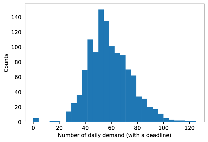
(a) With a deadline

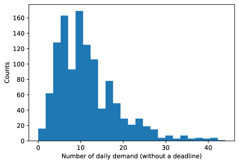
(b) Without a deadline

Figure 2: Histogram of the number of daily received orders across all zones, depending on whether the eviction orders have a deadline or not.

Table 1 presents the MLE results for the estimated mean and standard deviation of the arrival process for the entire system. For a more detailed discussion of the estimation method and the results for each individual zone, see Appendix LABEL:subapp:DemandEstimation.

Order type	Mean	Standard deviation
With a deadline	58.68	16.43
Without a deadline	11.63	7.16

Table 1: Estimated mean and standard deviation of the total arrivals per day.

Estimation of the order cancellation rate.

For simplicity, we estimate a common cancellation rate. Recall that the eviction orders received can be canceled before they are served. To estimate the cancellation rate, we apply a Kaplan-Meier estimator with bias correction, as detailed by Stute and Wang (1994). In our estimation, orders that are canceled are treated as uncensored observations, while those that are served are considered censored observations. The estimated cancellation rate is 0.0080 per day. A detailed discussion of the method and the results are included in Appendix LABEL:subapp:CancellationRateEstimation.

Estimation of eviction enforcement duration (not including travel times).

When a team of deputies arrives at the address of a pending eviction order, a non-negligible time period is required to enforce the order, i.e., the service time. We estimate the service time by calculating the difference between the recorded eviction start time and end time. Figure 3 shows the histogram of the service time recorded from the data.

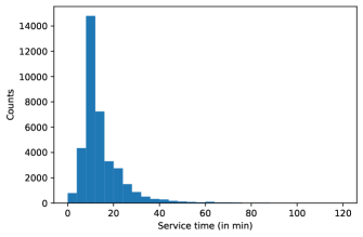
Figure 3: Empirical distribution of the service time of the eviction orders. The mean and standard deviation of the service time is 14.39 and 10.42 minutes, respectively.

To plan the route, we assume that each eviction order takes 14.39 minutes to enforce, based on the average service time derived from the CCSO dataset. When estimating the total working hours for each team in the simulation, we randomly select a service time for each served order using the empirical distribution of service times from the CCSO data, as shown in Figure 3. A detailed discussion of the estimation is provided in Appendix LABEL:subapp:ServiceTimeEstimation.

Estimation of the average number of eviction teams and their availability.

The number of eviction teams dispatched for daily enforcement assignments varies. Figure 4 shows the histogram of the number of teams assigned each day in the CCSO dataset. For our simulation study, we assume the number of teams for each daily assignment is 4, which corresponds to the average number of teams observed in the data. Appendix LABEL:subapp:NumTeamEstimation provides further details for this estimation.

Figure 4: Number of the teams for daily assignments throughout the history. The mean, median, and standard deviation of the number of teams in a daily assignment is 3.8722, 4, and 1.6408, respectively.

To estimate the daily working hours for each team, we first calculate the total number of working hours throughout the entire dataset. This information is obtained using the recorded eviction start and end time of the served eviction orders of each team. The estimated daily working hours are then determined by dividing the total working hours by the estimated average number of teams. Based on our calculations, each team is estimated to work approximately 5 hours per day. For a detailed discussion of the estimation, please refer to Appendix LABEL:subapp:DailyWorkingHoursEstimation.

Estimation of travel times.

The CCSO data does not include explicit information on travel times, but it does record the start and end times of each eviction order (for those that are enforced). While we can obtain the routes of the eviction enforcement from the CCSO data, we cannot directly use the time gap between the end of one order and the start of the next as the travel time for two key reasons: (1) In our proposed policy and the benchmark policies, it is possible that some routes not present in the CCSO data are recommended, leaving us with no information on travel times for those routes, and (2) travel times can vary significantly throughout the day (e.g., rush hours may lead to longer travel times), a factor that cannot be inferred directly from the data. To address these issues, we use a simple linear regression to estimate the travel time. Specifically, we first obtain the routes of the eviction enforcement from the CCSO data, treating each pair of consecutively enforced orders as a data point. Each data point has two attributes: (1) the distance difference, which is computed based on the geographical distance between the two orders, and (2) the travel time difference, which is calculated as the time gap between the eviction end time of the former order and the eviction start time of the latter order. Then the regression model is given by:

$${travel\;time} =\beta\times{distance},$$

where $\beta$ is the parameter to be estimated. Our estimation yields $\beta=1.9792$, with travel time and distance measured in minutes and kilometers, respectively. We provide a detailed discussion of the travel time estimation in Appendix LABEL:subapp:TravelTimeEstimation.

Estimation of the deadline.

As discussed in Section 3, the eviction orders of class $k$, where $k=1,\ldots,K$, have a deadline, which corresponds to the maximum time length until the order can be served. In the case of the Cook county, a deadline is typically set at 120 calendar days (which is approximately 85 workdays) after the judge issues the eviction order. However, there can be a delay between this approval and the receipt of the order by the CCSO for enforcement, which shorten the actual time duration until an order can be served. We estimate deadlines based on the duration between the received date and the assigned deadline from the data set. Figure 5 shows the distribution of these duration, where we focus on the number of workdays. For the simulation study, we generate each order’s deadline randomly based on this empirical distribution.

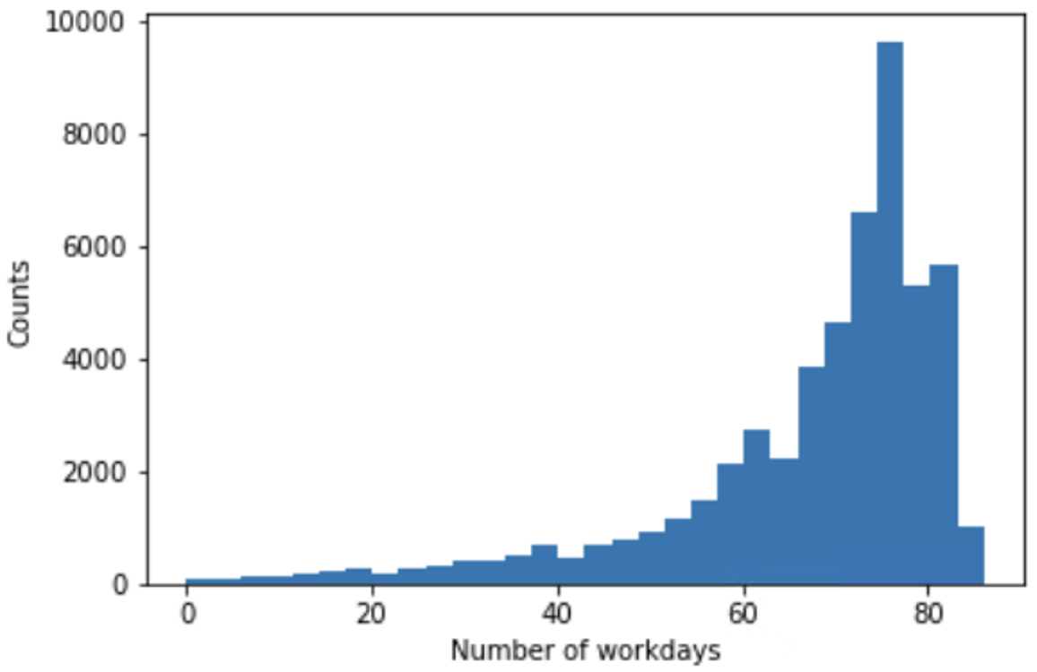
Figure 5: Distribution of the duration between the deadline and received date. The mean, median, and standard deviation is 69.17, 72, and 12.64, respectively.

7.2 Simulation Study

In this section, we compare the performance of our proposed policy against the two benchmark policies introduced in Section 6. Table 2 provides a summary of the performance measures used for comparison and their descriptions; see Appendix LABEL:app:PerformanceMeasures further details.

Performance	Description
Missing deadline percentage	The percentage of the orders that are not served nor canceled prior to their deadline.
Cancellation percentage	The percentage of the orders that are canceled (prior to their deadline). We report this metric for orders with or without a deadline separately.
Average number of orders waiting to be enforced	Number of orders that are waiting for service. We report this metric for orders with or without a deadline separately.
Number of orders served daily	Average number of orders that are served per day. We report this metric for orders with or without a deadline separately.

Table 2: Performance metrics.

In the simulation study, one can vary several operational levers. First, the cost parameters $c_{1},c_{2}$, and $p$ should be chosen so that the relative importance of reducing the number of pending orders and avoiding missing the deadline are reflected. Then, for the sake of computational efficiency, it is more practical to focus on a subset of pending orders with longer pending duration during daily planning, rather than considering all pending orders. The performance of the policies considered can depend on the specific size of this selected subset. In order to counteract this effect, we opt for a substantial subset, such as 500 orders that have the highest prizes. We determine this number so that results do not change significantly beyond this value. We refer to this number as the service threshold. In the remainder of this section, we first compare our proposed policy with the benchmark policies and then investigate on how different operational factors affect the performance of the proposed policy. In the simulation, we set the run length of all the experiments as 2000 simulated workdays, i.e., about eight years.

7.2.1 Comparison Between Proposed Policy and Benchmarks

Without loss of generality, we set $p=1$. Since $c_{1}$ represents the holding cost per pending day for each order with a deadline, and the deadline ranges approximately from 0 to 85 calendar days (see Figure 5), it is reasonable to assume $c_{1}<p/85$. In our experiments, we set $c_{1}=p/200=0.005$. The parameter $c_{2}$ represents the holding cost per day for orders without a deadline. The relative magnitude of $c_{1}$ and $c_{2}$ affect the allocation of service effort between orders with and without deadlines. A higher $c_{2}$ means that the holding cost for orders without a deadline increases, leading to more such orders being served. For our experiments, we let $h=c_{2}/c_{1}$, the ratio of the daily holding cost for orders with and without deadlines, and consider $h\in\{1,2,\ldots,10\}$. Note that $h=1$ implies equal holding costs for both orders with and without a deadline. Since orders with missed deadlines incur a penalty cost $p$, a great majority of the service effort is allocated to orders with deadlines in this case. Therefore, we do not consider $h<1$. In addition, we select $\xi=190$ and $w=0.3$ for the threshold-based policy and set $\tilde{d}=143$ for the urgency-based policy. These parameter values are calibrated using the CCSO dataset; see Appendix LABEL:app:ModelCalibration for further details.

Effect of the service effort allocation on the percentage of eviction orders that miss their deadline.

A larger holding cost ratio $h$ increases the service effort allocated to the eviction orders without a deadline. Figure 6 shows how the number of eviction orders with (Figure 6(a)) and without (Figure 6(b)) a deadline served changes as one varies $h$. It also shows how the percentage of eviction orders that miss their deadline varies (Figure 6(c)).

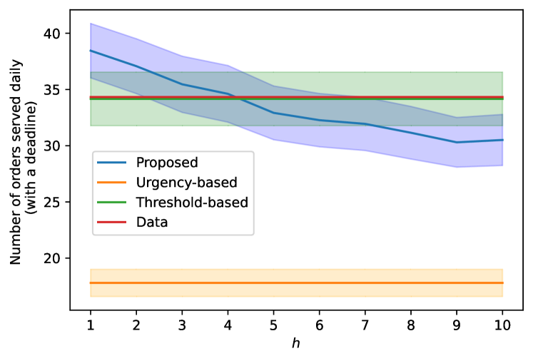
(a)

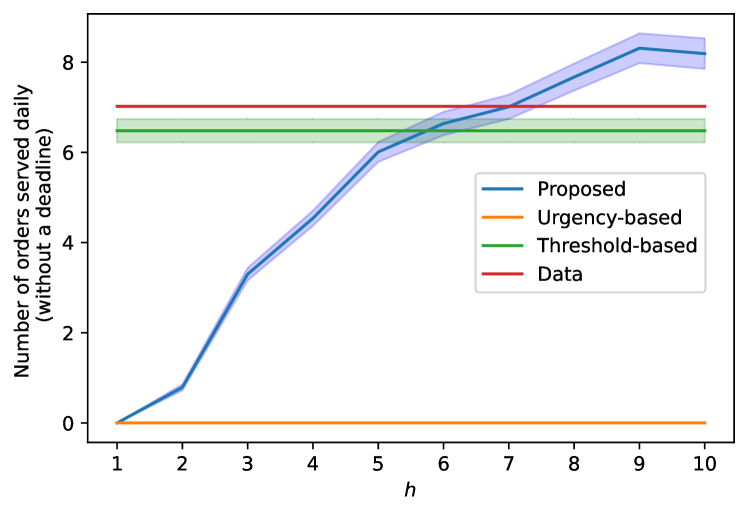
(b)

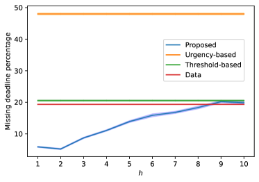
(c)

Figure 6: The number of orders served daily and missing deadline percentage for the two benchmark policies, the data, and the proposed policy in terms of $h\in\{1,2,\ldots,10\}$. The shaded area represents the 95% confidence interval estimated by 10 macro-replications through our simulation. Note that some results have narrow confidence intervals that are not visible in the figure.

We observe that the number of eviction orders enforced per day is close to that in the CCSO data under the proposed policy when $h=4$, but it significantly lowers the percentage of eviction orders that miss their deadline (by about 73%). Thus the holding cost parameter $h$ helps one balance the concerns of missing the deadline versus giving sufficient service attention to eviction orders without a deadline.

Trade-off between the percentage of eviction orders that miss their deadline and the cancellation percentage for eviction orders without a deadline.

As the holding cost ratio parameter $h$ increases, the service effort allocated to the eviction orders with a deadline decreases. As one would expect, this leads to larger percentage of eviction orders missing their deadline and a larger percentage of the orders with a deadline being canceled. More interestingly, Figure 7 shows the trade off (as $h$ varies) between the missing deadline percentage and the cancellation percentage (for orders without a deadline) as well as the average age of those orders before cancellation.

(a) Cancellation percentage (without deadline)

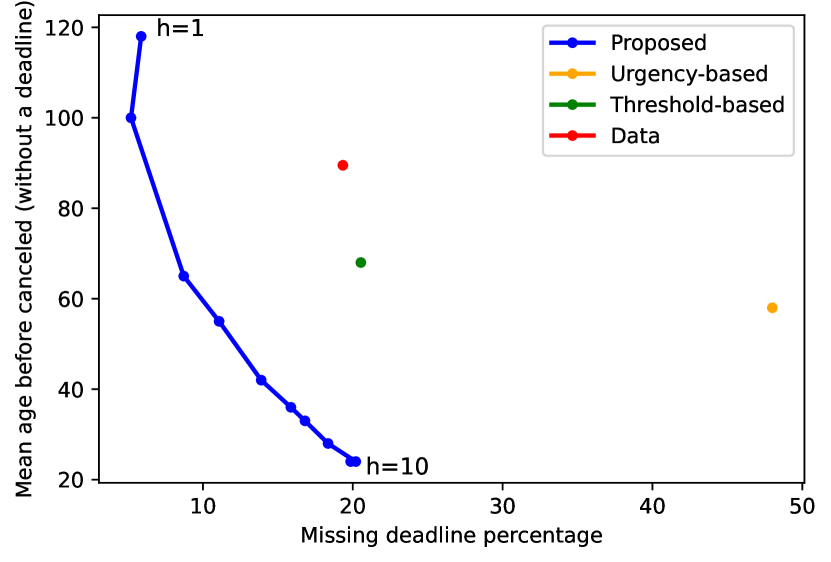
(b) Age before canceled (without deadline)

Figure 7: Trade-off curves for the missing deadline percentage against the cancellation percentage (without deadline) and the age of the orders (without deadline) before canceled for the proposed policy with different holding cost, the urgency-based policy, and the threshold-based policy.

As mentioned in Section 3, cancellations are not necessarily an undesirable outcome, as certain orders might be resolved by reaching an agreement between the tenant and the landlord. We further include the trade-off curve of the percentage of cancellation between the orders with and without a deadline in Figure 8.

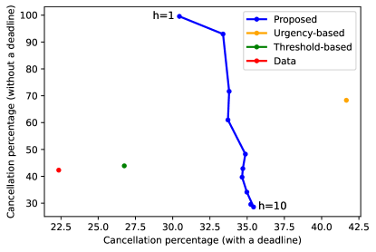
Figure 8: Relationship between the orders with and without deadlines in terms of the cancellation percentage.

Trade-off between missing deadline percentage and the number of orders pending.

As the holding cost ratio $h$ increases, more resources are diverted to enforcing the eviction orders without a deadline. Clearly, both the percentage of eviction orders missing their deadline and their number in the system increase in that case. Figure 9(a) shows the trade-off between the percentage missing their deadline and the number of pending orders without a deadline. Similarly, Figure 9(b) shows the trade-off between the number of pending eviction orders of two types (with or without a deadline) as $h$ varies.

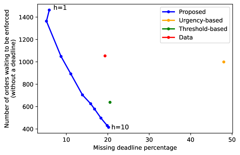
(a) Trade-off for missing deadline percentage

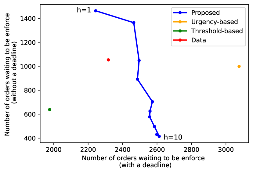
(b) Trade-off for number of orders waiting to be enforced (with deadline)

Figure 9: Trade-off between the number of orders without a deadline waiting to be enforced with respect to the percentage of orders that miss their deadline and the number of pending orders with a deadline.

In summary, as more service effort is diverted from the eviction orders with a deadline to those without a deadline (by increasing $h$), we observe the performance metrics (cancellation percentage, missing deadline percentage, and the number of pending orders) for the orders with a deadline gets slightly worse, whereas the performance metrics for the orders without a deadline improve dramatically. This is reflected by the steep nature of the trade-off curves in Figures 7–9, and it can guide decision making in practice.

7.2.2 Counterfactual Analysis

In this section, we conduct the counterfactual analysis of three counterfactual scenarios that vary the number of eviction teams, the number of daily working hours, or the deadline duration. In our experiments, we consider $h=4$ for the proposed policy, because it yields a similar number of daily served orders compared with that of the CCSO data.

As one would expect, increasing service capacity by increasing the number of eviction teams leads to improvements across the board. Figures 10–13 quantify the magnitudes of these improvements, which, of course, should be weighted against the capacity investment costs. In general, for all three policies, we observe that the percentage of missing deadline orders decreases, whereas the percentage of cancellation decreases, the number of daily served orders increases, and the number of daily pending orders decreases, as the number of vehicles increases.

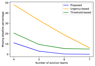
Figure 10: Missing deadline percentage as a function of eviction teams.

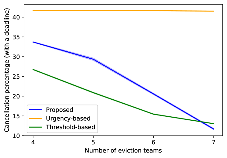
(a) With a deadline

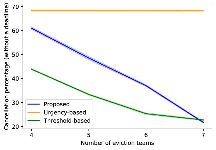
(b) Without a deadline

Figure 11: Cancellation percentage as a function of eviction teams.

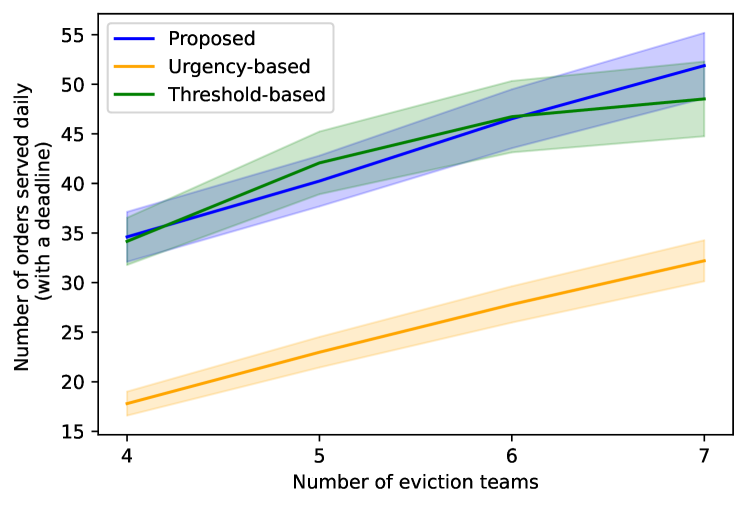
(a) With a deadline

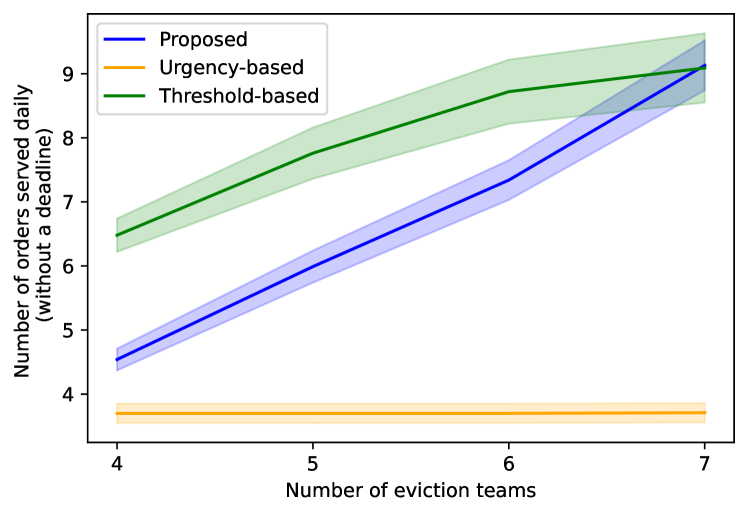
(b) Without a deadline

Figure 12: Number of orders served daily as a function of eviction teams.

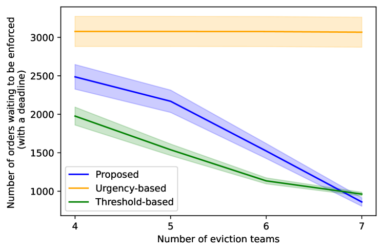
(a) With a deadline

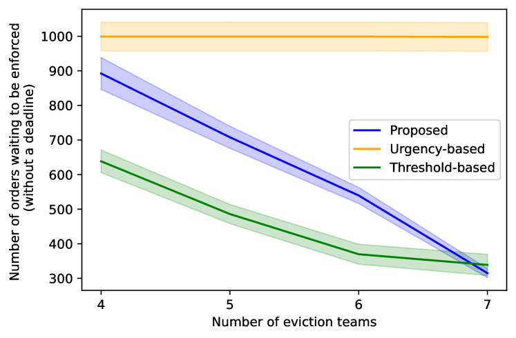
(b) Without a deadline

Figure 13: Number of orders waiting to be served in terms as a function of eviction teams.

Next, we consider a more granular adjustment to the service capacity. Namely, we study the effect of increasing the number of hours worked in a day for each vehicle, and observe a similar effect as when the number of eviction teams increases; see Figures 14–17.

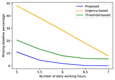
Figure 14: Missing deadline percentage as a function of daily working hours.

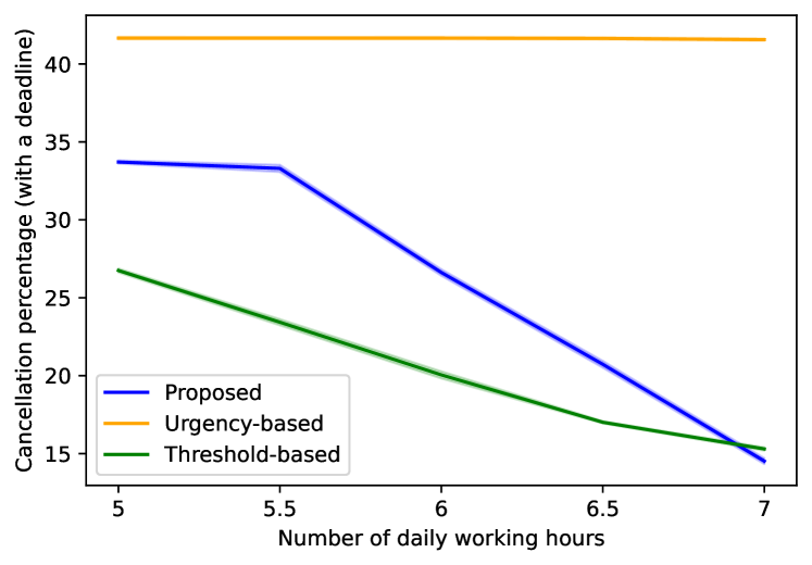
(a) With a deadline

(b) Without a deadline

Figure 15: Cancellation percentage as a function of daily working hours.

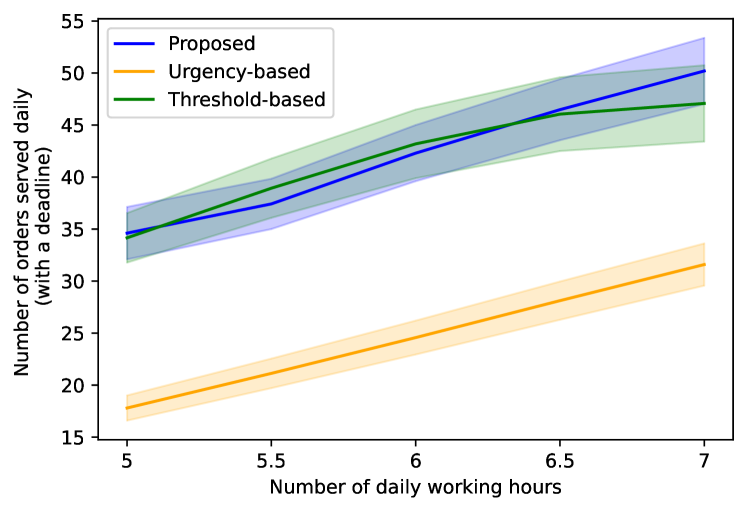
(a) With a deadline

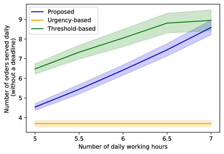
(b) Without a deadline

Figure 16: Number of orders served daily as a function of daily working hours.

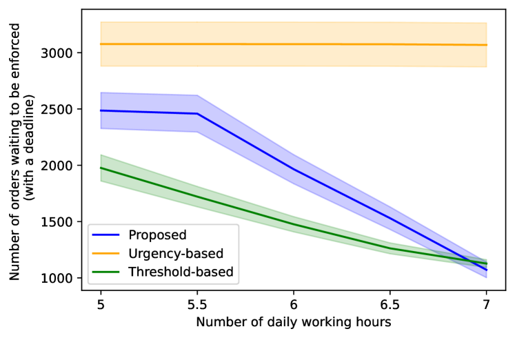
(a) With a deadline

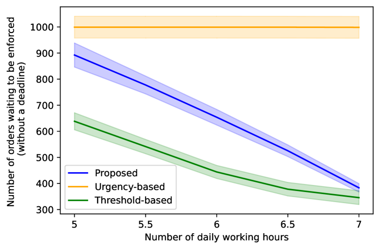
(b) Without a deadline

Figure 17: Number of orders waiting to be served as a function of daily working hours.

Finally, we present the effects of extending the deadline by an additional 10, 20, and 30 days; see Figures 18–21. We observe that the percentage of missing deadline decreases as the deadline is extended longer. On the other hand, the cancellation percentage for the orders with a deadline increases as the deadline is extended longer, which is expected as a longer deadline gives those orders a higher chance to be canceled. Another interesting finding is that the proposed policy results in a higher number of daily served orders without a deadline as the deadline of other orders is extended longer. This is due to the fact that the proposed policy assigns a higher prize to the orders with a deadline when the deadline approaches. When the deadline is extended, it assigns them a higher prize later that results in shifting the service effort slightly to the orders without a deadline.

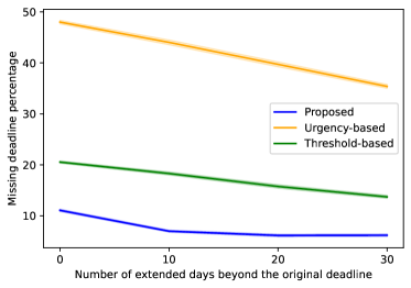
Figure 18: Missing deadline percentage as a function of daily working hours.

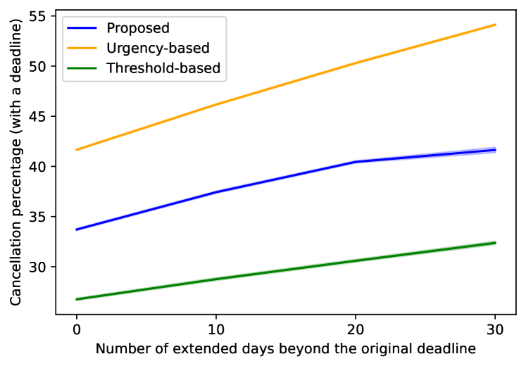
(a) With a deadline

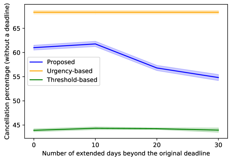
(b) Without a deadline

Figure 19: Cancellation percentage as a function of daily working hours.

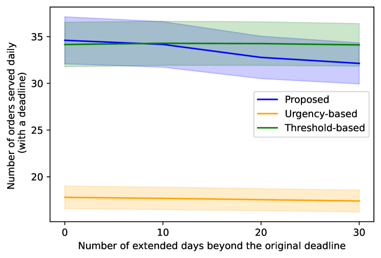
(a) With a deadline

(b) Without a deadline

Figure 20: Number of orders served daily as a function of daily working hours.

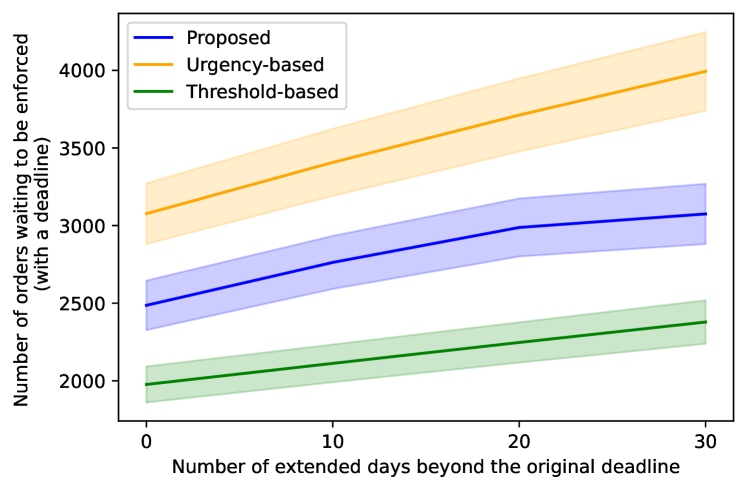
(a) With a deadline

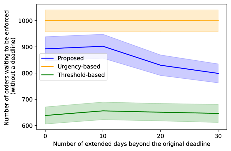
(b) Without a deadline

Figure 21: Number of orders waiting to be enforced in terms of different number of daily working hours.

8 Concluding Remarks

Our study is motivated by the eviction enforcement operations and the data from the CCSO, where the system manager must balance geographical coverage (as pending orders span the entirety of Cook County) and time constraints (as most eviction orders come with an enforcement deadline) when planning daily eviction operations, including the selection of orders to serve and the route to follow. Additionally, daily orders arrive with uncertainty, and cancellations are possible, which should be considered so that the daily decision is not myopic. When facing the trade-off between “equity” and “efficiency” in eviction enforcement planning, a FCFS policy, which emphasizes equity, may result in serving geographical dispersed orders on each day, thereby wasting resources. Conversely, focusing mainly on nearby orders to improve efficiency can increase the percentage of orders missing their deadlines.

To address this trade-off, we propose a policy and compare it with two benchmark policies and with the CCSO data. Our proposed approach selects orders and routes endogenously by solving a budgeted prize-collecting VRP, where the prize is determined by solving a Brownian control problem. This policy also allows the decision maker to adjust service effort between orders with and without deadlines by setting relative holding costs for each type. Our results show that the proposed policy reduces the percentage of missed deadlines by 72.38% compared to the CCSO data and also outperforms the benchmark policies. Notably, minimizing missing deadlines percentage requires prioritizing orders with deadlines, which leads to a higher cancellation rates by about 50%. This is because service efforts are more effectively directed toward orders nearing their deadlines, giving other orders more time to self-resolve (i.e., through cancellation), which can be a more desired outcome. Recall that a cancellation is not necessarily an undesirable outcome as it is often due to the landlord and the tenant reaching an agreement. Moreover, by adjusting the holding cost for each order type, the system manager can manage the trade-offs in cancellation rates and the number of orders waiting. These trade-offs also provide insights for eviction enforcement planning; see Figures 7–9.

We also conduct a counterfactual analysis to explore scenarios with increased service capacity (through more eviction teams and extended working hours) and with extended deadlines. Our results show that missed deadlines can be further reduced in both scenarios, but for different reasons. With increased service capacity, more orders are served, leading to lower cancellation rates and smaller number of orders waiting to be enforced. Conversely, extending deadlines reduces missed deadlines by allowing orders to stay longer in the system, which increases both the cancellation rate and the number of pending orders.

Lastly, it is worth noting that the data used in Section 7 is collected during 2015 – 2019, i.e., before the pandemic. During the pandemic, CCSO’s eviction operation were disrupted. As a result, our data set may not represent the current system state. Thus, we emphasize that our numerical study represents the CCSO’s eviction operations during 2015 – 2019 and its conclusions should be interpreted in that context.

Appendix

Appendix A Detailed Description of Solving Budgeted Prize-Collecting VRP

In this section, we first present related preliminary work related to solving the budgeted prize-collecting TSP in Appendix A.1. We then provide a detailed description of our proposed method of solving the budgeted prize-collecting VRP in Appendix A.2. Appendix A.3 includes a detailed discussion on constructing one of the inputs for the proposed algorithm. Finally, we provide implementation details for our numerical study based on the CCSO dataset in Appendix A.4.

A.1 Preliminaries

As discussed in Section 1 and 4.1, the algorithm presented by Hegde et al. [2015a] is computational efficient compared with other existing methods. Given that approximating function $H(z,v)$ requires a large number of data points and computational efficiency is crucial, our method utilizes one of the main algorithms in Hegde et al. [2015a].

Hegde et al. [2015a] consider a so-called Prize-Collecting Steiner Tree (PCST) problem, which, while different from our problem, is closely related. Loosely speaking, PCST aims to identify a subtree of a weighted graph that optimally balances the trade-off between the cost of the edges in the selected subtree and the prizes associated with the unconnected vertices. More specifically, we let $G=(V,E)$ be a connected, undirected, and weighted graph with edge costs $c:E\rightarrow\mathbb{R}_{0}^{+}$ and vertex prizes $\pi:V\rightarrow\mathbb{R}_{0}^{+}$. For any subgraph with vertices $V^{\prime}\subseteq V$ and edges $E^{\prime}\subseteq E$, we let the total prize of $V^{\prime}$ as $\pi(V^{\prime})=\sum_{v\in V^{\prime}}\pi(v)$ and the total cost of $E^{\prime}$ as $c(E^{\prime})=\sum_{e\in E^{\prime}}c(e)$. We further let $\overline{V^{\prime}}=V\setminus V^{\prime}$. Definition 1 provides the PCST problem definition studied by Hegde et al. [2015a].

Definition 1 (PCST problem).

Find a subtree $T=(V^{\prime},E^{\prime})$ of $G$ such that $c(E^{\prime})+\pi(\overline{V^{\prime}})$ is minimized.

Building on the work of Goemans and Williamson [1995] and Cole et al. [2001], Hegde et al. [2015a] present an algorithm, named PCST-FAST, that solves the PSCT in nearly linear time. PCST-FAST takes three parameters: the undirected graph $G=(V,E)$, the edge cost $c_{ij}\geq 0$ for $i,j\in V$ with $i\not=j$, and the vertex prize $\pi_{i}$ for $i\in V$. Since the focus of our work is not on the implementation details of PCST-FAST, we omit its algorithm description here. Interested reader may refer to Hegde et al. [2015a] for more details.

Although the goal of the PCST problem appears similar to our problem when a single vehicle is available, the resulting solution is a tree, whereas our problem aims to identify a tour for each vehicle. Following the method discussed in Goemans and Williamson [1995], we convert the identified tree from the PCST solution into a tour. That is, to solve the prize-collecting TSP (PCTSP), we first apply PCST-FAST and then convert the resulting tree into a tour as the solution to the PCTSP. Algorithm A.1 provides the detailed algorithmic statement of solving PCTSP.

Algorithm A.1 Solving the PCTSP

Input: An undirected graph $G=(V,E)$, edge costs $c_{ij}\geq 0$ for $i,j\in V$ and $i\not=j$, vertex prize $\pi_{i}\geq 0$ for $i\in V$, and a root vertex $r$.

Output: A tour $T$, which includes vertex $r\in V$.

1:function PCTSP($G,c,\pi,r$)

2:  Apply $\text{PCST-FAST}(G,c,\pi^{\prime},r)$ to the problem instance with graph $G$, edge costs $c$, root $r$, and prizes $\pi_{i}^{\prime}=\pi_{i}/2$ for $i\in V$. Obtain the solution as a subgraph $F$.

3:  Duplicate the edges of $F$ to form an Eulerian graph $F^{\prime}$.

4:  Form an Eulerian circuit in $F^{\prime}$ and then make the identified Eulerian circuit into a Hamiltonian circuit $T$ by skipping repeated vertices (shortcutting).

5:  return $T$

6:end function

A.2 Algorithm to Solve Budgeted Prize-Collecting VRP

To solve the budgeted prize-collecting VRP, we build on Algorithm A.1 with two additional requirement: i) the total travel and service time of each vehicle cannot exceed the maximum daily working hours, and ii) multiple vehicles are considered. First, we discuss a proposed procedure that addresses the budget constraint on travel costs when a single vehicle is considered. We then discuss how this procedure can be modified to incorporate multiple vehicles.

Budget constraint on edge cost.

To account for both travel time and service time, we assign the cost of each edge $e=(i,j)$, where $i,j\in V$ are the two vertices connected by $e$, as the sum of the travel time on edge $e$ and the service time required for serving the order at vertex $j$; see Section 7.1 for details on how travel time and service time are estimated. Recall from Definition 1 that the tour $T=(E^{\prime},V^{\prime})$ identified by Algorithm A.1 aims to minimize $c(E^{\prime})+\pi(\overline{V^{\prime}})$. However, this objective does not fully match our goal of maximizing $\pi(V^{\prime})$ (which is equivalent to minimizing $\pi(\overline{V^{\prime}})$) while also enforcing a constraint that $c(E^{\prime})$ remains below the maximum daily working hours.

To address this, inspired by Hegde et al. [2015b], we introduce a scaling parameter $\zeta>0$ that adjusts the prizes associated to all vertices through iterations updates by modifying the prize as $\zeta\pi_{i}$ for order $i\in V$. One may see that $\zeta$ needs to be neither too large nor too small. If $\zeta$ is significantly large, the algorithm prioritizes obtaining higher total reward over minimizing total travel cost, making the identified tour more likely to violate the budget constraint on edge cost. Conversely, if $\zeta$ is too small, satisfying the budget constraint on edge cost becomes more important than collecting a higher total prize, making it more likely to return a tour with few jobs (or even an empty tour). To find a $\zeta$ that effectively balance both vertex prizes and edge costs, we use a binary search method, ensuring that the identified tour satisfies the budget constraint on edge cost. Algorithm A.2 provides the algorithmic statement for solving the budgeted prize-collecting TSP.

Algorithm A.2 Budgeted-PCTSP

Input: An undirected graph $G=(V,E)$, edge costs $c_{ij}\geq 0$ for $i,j\in V$ with $i\not=j$, initial vertex prize $\pi_{i}\geq 0$ for $i\in V$, and a root vertex $r$. An initial value of the scaling parameter $\zeta^{\rm init}>0$ and the common edge cost budget $D$ for each vehicle. Tolerance level $\delta>0$ and tolerated precision $\epsilon>0$.

Output: A tour $T=(V_{T},E_{T})$, where $V_{T}\subseteq V$ with $r\in V_{T}$ and $E_{T}\subseteq E$.

1:function Budgeted-PCTSP($G,c,\pi,r,D,\zeta^{\rm init},\delta,\epsilon$)

2:  $\zeta_{l}\leftarrow 0$

3:  $\zeta_{r}\leftarrow\zeta_{\rm init}$

4:  $T=(V_{T},E_{T})\leftarrow\textsc{PCTSP}(G,c,\zeta_{r}\cdot\pi,r)$

5:  if $|c(E_{T})-D|\leq\delta$ then

6:   return $T=(V_{T},E_{T})$

7:  end if

8:  while ($|c(E_{T})-D|>\delta$) and ($\zeta_{r}-\zeta_{l}>\epsilon$) do

9:   $\zeta_{m}\leftarrow(\zeta_{l}+\zeta_{r})/2$

10:   $T=(V_{T},E_{T})\leftarrow\textsc{PCTSP}(G,c,\zeta_{m}\cdot\pi,r)$

11:   if $c(E_{T})<D-\delta$ then

12:     $\zeta_{r}\leftarrow\zeta_{m}$

13:   else

14:     $\zeta_{l}\leftarrow\zeta_{m}$

15:   end if

16:  end while

17:  if $|c(T)-D|\leq\delta$ then

18:   return $T=(V_{T},E_{T})$

19:  else

20:   $T_{l}=(V_{T_{l}},E_{T_{l}})\leftarrow\textsc{PCTSP}(G,c,\zeta_{l}\cdot\pi,r)$

21:   $T_{r}=(V_{T_{r}},E_{T_{r}})\leftarrow\textsc{PCTSP}(G,c,\zeta_{r}\cdot\pi,r)$

22:   $c^{T_{r}}\leftarrow\{\}$

23:   for $i\leftarrow 1,\ldots,|V_{T_{r}}|-1$ do

24:     $c^{T_{r}}\leftarrow c^{T_{r}}\cup\{c_{v_{i},v_{i+1}}\}$

25:   end for

26:   $T_{r}^{\prime}=(V_{T_{r}^{\prime}},E_{T_{r}^{\prime}})\leftarrow\textsc{PruneTour}(T_{r},c^{T_{r}},D,\delta,r)$

27:   if $\pi(V_{T_{l}})\geq\pi(V_{T_{r}^{\prime}})$ then

28:     return $T_{l}$

29:   else

30:     return $T_{r}^{\prime}$

31:   end if

32:  end if

33:end function

Note that through the binary search over $\zeta$, it is possible that one of the resulting tours (i.e., the resulting tour corresponds to $\zeta_{r}$) significantly exceeds the edge cost budget, even if $\zeta_{l}$ and $\zeta_{r}$ are extremely close (i.e., $\zeta_{r}-\zeta_{l}\leq\epsilon$). To address this, we use a subroutine PruneTour to extract a subtour when such a situation occurs; see Algorithm A.3. Since the tour that violates the cost budget constraint is expected to include vertices with high prizes, PruneTour simply selects vertices along the tour, starting from the root vertex, and continues until the edge cost budget is exhausted.

Algorithm A.3 PruneTour

Input: A tour $T=(V_{T},E_{T})$, edge costs $c_{ij}\geq 0$ for $i,j\in V_{T}$ with $i\not=j$, the edge cost budget $D$, and a root vertex $r$. Tolerance level $\delta>0$.

Output: A pruned tour $T^{\prime}=(V_{T^{\prime}},E_{T^{\prime}})$, where $V_{T^{\prime}}\subseteq V_{T}$ with $r\in V_{T^{\prime}}$ and $E_{T^{\prime}}\subseteq E_{T}$.

1:function PruneTour($T,c,D,\delta,r$)

2:  Let $L=\{v_{1},v_{2},\ldots,v_{|V_{T}|},v_{1}\}$ be the tour of $T$, where $v_{1}$ is the root vertex $r$.

3:  if $c(V_{T})\leq D+\delta$ then

4:   return $T=(V_{T},E_{T})$

5:  end if

6:  $T^{\prime}\leftarrow\{v_{1}\}$

7:  for $i\leftarrow 2,\ldots,|V_{T}|$ do

8:   $T^{\prime}\leftarrow T^{\prime}\cup\{v_{i}\}$

9:   $b\leftarrow\sum_{i=1}^{|T^{\prime}|-1}c_{v_{i},v_{i+1}}$

10:   if $b>D+\delta$ then

11:     $V_{T^{\prime}}\leftarrow\left\{v_{1},\ldots,v_{i-1}\right\}$

12:     $E_{T^{\prime}}\leftarrow\cup_{i=1}^{|T^{\prime}|-1}\{(v_{i},v_{i+1})\}$

13:     return $T^{\prime}=(V_{T^{\prime}},E_{T^{\prime}})$

14:   end if

15:  end for

16:end function

Incorporating multiple vehicles.

To incorporate multiple vehicles, we repeatedly apply Algorithm A.2 for each vehicle with respect to the remaining orders, as the number of daily pending orders can be substantial.

Algorithm A.4 presents our proposed heuristic method for solving the budgeted prize-collecting VRP when facing a set of pending orders, denoted as ${\cal P}$. Each pending order in ${\cal P}$ includes information of the order, such as location (in latitude and longitude), pending duration, deadline, etc., which is used to determine the prize assigned based on the chosen policy; see detailed discussion in Appendix LABEL:subapp:PolicyDescription. Note that Algorithm A.4 requires two additional algorithms: CreateGraph, which generates a complete graph as input for Budgeted-PCTSP, and AssignPrize, which assigns prizes to the pending orders according to the chosen policy. Detailed discussion of CreateGraph and AssignPrize are provided in Appendices A.3 and LABEL:subapp:AssignPrize, respectively.

Algorithm A.4 Solution to the Budgeted-PCVRP

Input: Set of pending orders ${\cal P}$. A root vertex $r$. An initial value of the scaling parameter $\zeta^{\rm init}>0$. Number of vehicles $W$. Edge cost budget $D=\{D_{w}\mid w=1,\ldots,W\}$ for all vehicles. Tolerance level $\delta>0$ and tolerated precision $\epsilon>0$. The chosen policy and the required inputs (see Algorithm LABEL:alg:AssignPrize).

Output: A set of $W$ tours where all the tours include root vertex $r$.

1:function Budgeted-PCVRP(${\cal P},r,W,D,\zeta^{\rm init},\delta,\epsilon,{\rm policy}$)

2:  for $w\leftarrow 1,\ldots,W$ do

3:   $\pi\leftarrow\textsc{AssignPrize}({\rm policy},{\cal P},\text{Inputs for the chosen policy})$

4:   $G,\pi^{\rm init},c\leftarrow\textsc{CreateGraph}({\cal P},\pi)$

5:   $T_{w}=(V_{w},E_{w})\leftarrow\textsc{Budgeted-PCTSP}(G,c,\pi^{\rm init},r,D_{w},\zeta^{\rm init},\delta,\epsilon)$

6:   Remove orders whose location is within $V_{w}$ from ${\cal P}$

7:  end for

8:  return $\{T_{w}=(V_{w},E_{w})\mid w=1,\ldots,W\}$

9:end function

A.3 Construction of the Input Undirected Graph

A crucial step in Algorithm A.4 is the implementation of Budgeted-PCTSP, which requires an undirected graph along with the prizes for its vertices as part of the input. To create the input graph $G=(V,E)$, where $V$ is the set of vertices and $E$ is the set edges connecting these vertices, we obtain the information for $V$ and $E$ from the daily pending orders. As discussed in Appendix A.2, we let ${\cal P}$ be the set of pending orders, which includes essential location information (latitude and longitude) for each order. To determine the cost of an edge $(i,j)$, where $i,j\in V$, we first compute the estimated travel time for the edge using the estimation in Section 7.1. We then add the average service time, also estimated in Section 7.1, since the total cost for traveling from vertex $i$ to vertex $j$ and completing enforcement at vertex $j$ constitutes the total cost of edge $(i,j)$. Furthermore, prior to creating the input graph $G$, the system manager generates a prize for each pending order $i\in{\cal P}$ based on the chosen policy. We denote these generated prizes as $\pi_{\rm pending}$ and assign them accordingly to the vertices in graph $G$. Algorithm A.5 shows the procedure for constructing the input graph $G=(V,E)$.

Algorithm A.5 Input graph creation

Input: Set of pending orders ${\cal P}$. The prize vector $\pi$, where $\pi_{i}$ corresponds to the prize for order $i\in{\cal P}$.

Output: Graph $G=(V,E)$, vertex prize $\pi_{i}$ for $i\in V$, and edge cost $c_{ij}$ for the edge in between of $i,j\in V$ and $i\not=j$.

1:function GraphCreation(${\cal P},\pi$)

2:  $V\leftarrow\{\}$

3:  $E\leftarrow\{\}$

4:  for $i=({\rm lat}_{i},{\rm lng}_{i},\ell^{\rm pending}_{i},t^{\rm cancel}_{i},t^{\rm deadline}_{i},{\rm class}_{i})\in{\cal P}$ do

5:   $V\leftarrow V\cup\{i\}$

6:   for $j=({\rm lat}_{j},{\rm lng}_{j},\ell^{\rm pending}_{j},t^{\rm cancel}_{j},t^{\rm deadline}_{j},{\rm class}_{j})\in{\cal P}$ where $i\not=j$ do

7:     $E\leftarrow E\cup\{(i,j)\}$

8:     $d_{ij}\leftarrow$ Haversine distance between $({\rm lat}_{i},{\rm lng}_{i})$ and $({\rm lat}_{j},{\rm lng}_{j})$

9:     $c_{ij}\leftarrow\beta d_{ij}+t_{service}$, where $t_{service}$ is the average service time (see Section 7.1)

10:   end for

11:  end for

12:  return $G=(V,E),\pi_{i}$ for $i\in V$, and $c_{ij}$ for $i,j\in V$ and $i\not=j$

13:end function

A.4 Implementation Details on the CCSO Eviction Data

In this section, we discuss our choices and adjustments for some inputs to Budgeted-PCTSP.

Adjustment for $\pi^{\rm init}$.

To balance the priority values of the pending orders across all policies, we scale the initial prizes, $\pi^{\rm init}$, through a binary search of $\zeta$ to align them with the edge cost. Since the prizes determined by each policy are initially much smaller than the edge cost, we multiply them by 1,000,000. This scaling factor ensures that the prizes are significantly larger than the edge cost, preserving the relative differences between the prizes. Note that other scaling factors may also be considered, and the results are not expected to change.

Adjustment for edge cost $c$.

Based on the CCSO dataset, we observe that some eviction requests can be very close, such as within nearby buildings or even the same building. In these cases, the edge cost $c_{ij}$ would be extremely small. However, in practice, deputies are still expected to spend time traveling between two closely located orders. To account for this, we set a minimum edge cost of 5 minutes when creating the input graph, as described in Algorithm A.5.

Choice of $\zeta^{\rm init}$.

The value of $\zeta^{\rm init}$ depends on the order of magnitude difference between the assigned initial prize $\pi^{\rm init}$ and the edge cost $c$. In our simulation study, we set $\zeta^{\rm init}=100$.

Choice of $\delta$.

The tolerate level $\delta$ serves as a buffer for the edge cost budget. Specifically, Algorithm A.4 aims to find routes with an overall edge cost within $[D-\delta,D+\delta]$ with high probability, where $D$ is the user-defined edge cost budget. The choice of $\delta$ depends on how much deviation from $D$ is acceptable to the system manager. In our simulation study, we assume the CCSO is indifferent with respect to 30 minutes in terms of their daily working hour and set $\delta$ as 30 minutes.

Choice of $\epsilon$.

The tolerated precision $\epsilon$ measures the maximum allowable difference between the scaling parameters $\zeta_{l}$ and $\zeta_{r}$ through the binary search (see Algorithm A.2). A smaller $\epsilon$ requires a finer distinction between $\zeta_{l}$ and $\zeta_{r}$, leading to longer computational time. In our simulation study, we set $\epsilon=0.0001$.

Appendix B Additional Discussion on Approximating Function $H(z,v)$

In this section, we provide additional discussion on how we approximate $H(z,v)$ (discussed in Section 4.1). Appendix B.1 provides an overview and algorithm for approximating $H(z,v)$, followed by implementation details in Appendix LABEL:subapp:ResultsApproximationH.

B.1 Procedure to Approximate $H(z,v)$

We use a neural network model to approximate $H(z,v)$ because incorporating it in Algorithm 3 is easier. Completing this task involves two main steps: generating training data and training the neural network model.

Recall from Section 4.1 that $H(z,w)=\max_{\mu\in{\cal A}(z)}\{\mu z\}$, where $z$ and $v$ are $2K$-dimensional vectors representing the number of daily pending eviction orders and the prize of serving one eviction order from each class, respectively. Each training data point includes three elements: the $2K$-dimensional vectors $z$ and $v$, and the corresponding response $\max_{\mu\in{\cal A}(z)}\{\mu v\}$. This response is the maximum total prize collectable, or the solution to the budgeted prize-collecting VRP, where $z_{k}$ represents the number of pending orders for class $k$, and $v_{k}$ represents the prize of serving one order of class $k$.

To facilitate the discussion, we let $n_{k}^{\rm max}$ be the maximum number of pending orders from class $k$, as observed in the CCSO dataset, and let ${\cal O}_{k}$ be the set of historical order locations from the dataset. To generate one training data point, we proceed as follows:

1. We determine the number of pending orders for each class $z_{k}$ by generating a uniform random variable over the interval $[0,1.5n_{k}^{\rm max}]$.

2. Next, we randomly select $z_{k}$ locations from the set ${\cal O}_{k}$. For each selected order, we assign a prize by generating a uniform random variable over the interval $[0,p]$ if the order has a deadline, or $[0,h_{2}/\gamma_{k}]$ if it does not. These ranges are based on the boundary conditions in the HJB equation (Equations (12)–(14)).

3. Finally, solve the budgeted VRP to determine the maximum total prize collected $\max_{\mu\in{\cal A}(z)}\{\mu v\}$.

Algorithms 5 shows the algorithm for generating one training data point.

Algorithm A.6 Generate one training data point

Input: Set of locations of the historical orders ${\cal O}$. Penalty of missing deadline $p$. Holding cost of the orders without a deadline $h_{2}$. Cancellation rate of class $k$, $\gamma_{k}$, where $k=1,\ldots,2K$. Number of vehicles $W$. Edge cost budget $D=\{D_{w}\mid w=1,\ldots,W\}$. An initial value of the scaling parameter $\zeta^{\rm init}>0$, a root vertex $r$, tolerance level $\delta>0$, and tolerated precision $\epsilon>0$.

Output: Number of pending orders $z$, assigned prizes for all classes $v$, and total prize collected by all vehicles $p_{\rm total}$.

1:function DataGen(${\cal O},p,h_{2},\gamma,r,W,D,\zeta^{\rm init},\delta,\epsilon$)

2:  $V_{\rm pending}\leftarrow\{\}$

3:  $\pi_{\rm pending}\leftarrow\{\}$

4:  for $k=1,\ldots,2K$ do

5:   if $k\leq K$ then

6:     $v_{k}\leftarrow{\rm Unif}(0,p)$

7:   else

8:     $v_{k}\leftarrow{\rm Unif}(0,h_{2}/\gamma_{k})$

9:   end if

10:   $z_{k}\leftarrow{\rm Unif}(0,1.5n^{k}_{\max})$

11:   for $n=1,\ldots,z_{k}$ do

12:     $i_{n}\leftarrow$ Randomly chosen location $({\rm lat}_{n},{\rm lng}_{n})$ from ${\cal O}_{k}$

13:     $V_{\rm pending}\leftarrow V_{\rm pending}\cup\{i_{n}\}$

14:     $\pi_{\rm pending}\leftarrow\pi_{\rm pending}\cup\{v_{k}\}$

15:   end for

16:  end for

17:  $G,\pi^{\rm init},c\leftarrow\textsc{GraphCreation}(V_{\rm pending},\pi_{\rm pending})$

18:  for $w=1,\ldots,W$ do

19:   $T_{w}=(V_{w},E_{w})\leftarrow\textsc{Budgeted-PCTSP}(G,c,\pi^{\rm init},r,D,\zeta^{\rm init},\delta,\epsilon)$

20:  end for

21:  $p_{\rm total}\leftarrow\sum_{w=1}^{W}\pi(V_{w})$

22:  return $z,v,p_{\rm total}$

23:end function

References

- Albareda-Sambola et al. [2014] Maria Albareda-Sambola, Elena Fernández, and Gilbert Laporte. The dynamic multiperiod vehicle routing problem with probabilistic information. Computers & Operations Research, 48:31–39, 2014.
- Alwan et al. [2024] Amir A. Alwan, Baris Ata, and Yuwei Zhou. A queueing model of dynamic pricing and dispatch control for ride-hailing systems incorporating travel times. Queueing Systems, 106(1):1–66, 2024.
- Angelelli et al. [2007a] Enrico Angelelli, M. Grazia Speranza, and Martin W.P. Savelsbergh. Competitive analysis for dynamic multiperiod uncapacitated routing problems. Networks, 49(4):308–317, 2007a.
- Angelelli et al. [2007b] Enrico Angelelli, Martin W.P. Savelsbergh, and M. Grazia Speranza. Competitive analysis of a dispatch policy for a dynamic multi-period routing problem. Operations Research Letters, 35(6):713–721, 2007b.
- Ata [2006] Barış Ata. Dynamic control of a multiclass queue with thin arrival streams. Operations Research, 54(5):876–892, 2006.
- Ata and Barjesteh [2023] Baris Ata and Nasser Barjesteh. An approximate analysis of dynamic pricing, outsourcing, and scheduling policies for a multiclass make-to-stock queue in the heavy traffic regime. Operations Research, 71(1):341–357, 2023.
- Ata and Kasikaralar [2023] Baris Ata and Ebru Kasikaralar. Dynamic scheduling of a multiclass queue in the halfin-whitt regime: A computational approach for high-dimensional problems. Working paper, Univeristy of Chicago, 2023.
- Ata et al. [2019] Baris Ata, Deishin Lee, and Erkut Sönmez. Dynamic volunteer staffing in multicrop gleaning operations. Operations Research, 67(2):295–314, 2019.
- Ata et al. [2024a] Baris Ata, J. Michael Harrison, and Nian Si. Drift control of high-dimensional reflected brownian motion: A computational method based on neural networks. Stochastic Systems, 0(0):null, 2024a.
- Ata et al. [2024b] Baris Ata, J. Michael Harrison, and Nian Si. Singular control of (reflected) brownian motion: a computational method suitable for queueing applications. Queueing Systems, 108(3):215–251, 2024b.
- Ata et al. [2024c] Baris Ata, Deishin Lee, and Mustafa Hayri Tongarlak. A diffusion model of dynamic participant inflow management. Queueing Systems, 2024c.
- Ata et al. [2024d] Baris Ata, Mustafa H. Tongarlak, Deishin Lee, and Joy Field. A dynamic model for managing volunteer engagement. Operations Research, 2024d.
- Ata et al. [2005] Bariş Ata, J. M. Harrison, and L. A. Shepp. Drift rate control of a Brownian processing system. The Annals of Applied Probability, 15(2):1145 – 1160, 2005.
- Azi et al. [2012] Nabila Azi, Michel Gendreau, and Jean-Yves Potvin. A dynamic vehicle routing problem with multiple delivery routes. Annals of Operations Research, 199(1):103–112, 2012.
- Baldacci et al. [2023] Roberto Baldacci, Edna A. Hoshino, and Alessandro Hill. New pricing strategies and an effective exact solution framework for profit-oriented ring arborescence problems. European Journal of Operational Research, 307(2):538–553, 2023.
- Beck et al. [2023] Christian Beck, Martin Hutzenthaler, Arnulf Jentzen, and Benno Kuckuck. An overview on deep learning-based approximation methods for partial differential equations. Discrete and Continuous Dynamical Systems - B, 28(6):3697–3746, 2023.
- Bertsimas [1992] Dimitris J. Bertsimas. A vehicle routing problem with stochastic demand. Operations Research, 40(3):574–585, 1992.
- Carlsson et al. [2024] John Gunnar Carlsson, Sheng Liu, Nooshin Salari, and Han Yu. Provably good region partitioning for on-time last-mile delivery. Operations Research, 72(1):91–109, 2024.
- Çelik and Maglaras [2008] Sabri Çelik and Costis Maglaras. Dynamic pricing and lead-time quotation for a multiclass make-to-order queue. Management Science, 54(6):1132–1146, 2008.
- Chessari et al. [2023] Jared Chessari, Reiichiro Kawai, Yuji Shinozaki, and Toshihiro Yamada. Numerical methods for backward stochastic differential equations: A survey. Probability Surveys, 20, Jan 2023.
- Cole et al. [2001] Richard J. Cole, Ramesh Hariharan, Moshe Lewenstein, and Ely Porat. A faster implementation of the goemans-williamson clustering algorithm. In ACM-SIAM Symposium on Discrete Algorithms, 2001.
- Dantzig and Ramser [1959] G. B. Dantzig and J. H. Ramser. The truck dispatching problem. Management Science, 6(1):80–91, 1959.
- Desmond [2012] Matthew Desmond. Eviction and the reproduction of urban poverty. American Journal of Sociology, 118(1):88–133, 2012.
- Desmond [2022] Matthew Desmond. Unaffordable America: Poverty, housing, and eviction. 2022.
- E et al. [2021] Weinan E, Jiequn Han, and Arnulf Jentzen. Algorithms for solving high dimensional pdes: from nonlinear monte carlo to machine learning. Nonlinearity, 35(1):278, dec 2021.
- El-Hajj et al. [2016] Racha El-Hajj, Duc-Cuong Dang, and Aziz Moukrim. Solving the team orienteering problem with cutting planes. Computers & Operations Research, 74:21–30, 2016.
- Feillet et al. [2005] Dominique Feillet, Pierre Dejax, and Michel Gendreau. The profitable arc tour problem: Solution with a branch-and-price algorithm. Transportation Science, 39(4):539–552, 2005.
- Flatberg et al. [2007] Truls Flatberg, Geir Hasle, Oddvar Kloster, Eivind J. Nilssen, and Atle Riise. Dynamic And Stochastic Vehicle Routing In Practice, pages 41–63. Springer US, Boston, MA, 2007.
- Fleming and Soner [2006] Wendell H. Fleming and H.M. Soner. Controlled Markov Processes and Viscosity Solutions. Springer New York, NY, 2006.
- Flood [1956] Merrill M. Flood. The traveling-salesman problem. Operations Research, 4(1):61–75, 1956.
- Gendreau et al. [1996] Michel Gendreau, Gilbert Laporte, and René Séguin. Stochastic vehicle routing. European Journal of Operational Research, 88(1):3–12, 1996.
- Ghosh and Weerasinghe [2007] Arka P. Ghosh and Ananda P. Weerasinghe. Optimal buffer size for a stochastic processing network in heavy traffic. Queueing Systems, 55(3):147–159, 2007.
- Ghosh and Weerasinghe [2010] Arka P. Ghosh and Ananda P. Weerasinghe. Optimal buffer size and dynamic rate control for a queueing system with impatient customers in heavy traffic. Stochastic Processes and their Applications, 120(11):2103–2141, 2010.
- Gilbarg and Trudinger [2001] David Gilbarg and Neil S. Trudinger. Elliptic Partial Differential Equations of Second Order. Springer Berlin, Heidelberg, 2001.
- Goemans and Williamson [1995] Michel X. Goemans and David P. Williamson. A general approximation technique for constrained forest problems. SIAM Journal on Computing, 24(2):296–317, 1995.
- Goodson et al. [2013] Justin C. Goodson, Jeffrey W. Ohlmann, and Barrett W. Thomas. Rollout policies for dynamic solutions to the multivehicle routing problem with stochastic demand and duration limits. Operations Research, 61(1):138–154, 2013.
- Gromis et al. [2022] Ashley Gromis, Ian Fellows, James R. Hendrickson, Lavar Edmonds, Lillian Leung, Adam Porton, and Matthew Desmond. Estimating eviction prevalence across the united states. Proceedings of the National Academy of Sciences, 119(21):e2116169119, 2022.
- Han et al. [2018] Jiequn Han, Arnulf Jentzen, and Weinan E. Solving high-dimensional partial differential equations using deep learning. Proceedings of the National Academy of Sciences, 115(34):8505–8510, 2018.
- Harrison [1988] J. Michael Harrison. Brownian models of queueing networks with heterogeneous customer populations. In Wendell Fleming and Pierre-Louis Lions, editors, Stochastic Differential Systems, Stochastic Control Theory and Applications, pages 147–186, New York, NY, 1988. Springer New York.
- Harrison [2000] J. Michael Harrison. Brownian models of open processing networks: canonical representation of workload. The Annals of Applied Probability, 10(1):75 – 103, 2000.
- Harrison [2003] J. Michael Harrison. A broader view of Brownian networks. The Annals of Applied Probability, 13(3):1119 – 1150, 2003.
- Harrison [2013] J. Michael Harrison. Brownian Models of Performance and Control. Cambridge University Press, 2013.
- Harrison and Reiman [1981] J. Michael Harrison and Martin I. Reiman. On the distribution of multidimensional reflected brownian motion. SIAM Journal on Applied Mathematics, 41(2):345–361, 1981.
- Harrison and Wein [1989] J. Michael Harrison and Lawrence M. Wein. Scheduling networks of queues: Heavy traffic analysis of a simple open network. Queueing Systems, 5(4):265–279, 1989.
- Harrison and Wein [1990] J. Michael Harrison and Lawrence M. Wein. Scheduling networks of queues: Heavy traffic analysis of a two-station closed network. Operations Research, 38(6):1052–1064, 1990.
- Hegde et al. [2015a] Chinmay Hegde, Piotr Indyk, and Ludwig Schmidt. A fast , adaptive variant of the goemans-williamson scheme for the prize-collecting steiner tree problem. 2015a.
- Hegde et al. [2015b] Chinmay Hegde, Piotr Indyk, and Ludwig Schmidt. A nearly-linear time framework for graph-structured sparsity. In Proceedings of the 32nd International Conference on International Conference on Machine Learning - Volume 37, ICML’15, page 928–937. JMLR.org, 2015b.
- Keskin et al. [2023] Merve Keskin, Juergen Branke, Vladimir Deineko, and Arne K. Strauss. Dynamic multi-period vehicle routing with touting. European Journal of Operational Research, 310(1):168–184, 2023.
- Klapp et al. [2018] Mathias A. Klapp, Alan L. Erera, and Alejandro Toriello. The one-dimensional dynamic dispatch waves problem. Transportation Science, 52(2):402–415, 2018.
- Laporte et al. [1992] Gilbert Laporte, François Louveaux, and Hélène Mercure. The vehicle routing problem with stochastic travel times. Transportation Science, 26(3):161–170, 1992.
- Liu and Luo [2023] Sheng Liu and Zhixing Luo. On-demand delivery from stores: Dynamic dispatching and routing with random demand. Manufacturing & Service Operations Management, 25(2):595–612, 2023.
- Liu et al. [2021] Sheng Liu, Long He, and Zuo-Jun Max Shen. On-time last-mile delivery: Order assignment with travel-time predictors. Management Science, 67(7):4095–4119, 2021.
- Markowitz et al. [2000] David M. Markowitz, Martin I. Reiman, and Lawrence M. Wein. The stochastic economic lot scheduling problem: Heavy traffic analysis of dynamic cyclic policies. Operations Research, 48(1):136–154, 2000.
- Pessoa et al. [2020] Artur Pessoa, Ruslan Sadykov, Eduardo Uchoa, and François Vanderbeck. A generic exact solver for vehicle routing and related problems. Mathematical Programming, 183(1):483–523, 2020.
- Pillac et al. [2013] Victor Pillac, Michel Gendreau, Christelle Guéret, and Andrés L. Medaglia. A review of dynamic vehicle routing problems. European Journal of Operational Research, 225(1):1–11, 2013.
- Plambeck et al. [2001] Erica Plambeck, Sunil Kumar, and J. Michael Harrison. A multiclass queue in heavy traffic with throughput time constraints: Asymptotically optimal dynamic controls. Queueing Systems, 39(1):23–54, 2001.
- Pon [2023] Peter Pon. Private Communication, 2023.
- Reiman et al. [1999] Martin I. Reiman, Rodrigo Rubio, and Lawrence M. Wein. Heavy traffic analysis of the dynamic stochastic inventory-routing problem. Transportation Science, 33(4):361–380, 1999.
- Rubino and Ata [2009] Melanie Rubino and Baris Ata. Dynamic control of a make-to-order, parallel-server system with cancellations. Operations Research, 57(1):94–108, 2009.
- Secomandi and Margot [2009] Nicola Secomandi and François Margot. Reoptimization approaches for the vehicle-routing problem with stochastic demands. Operations Research, 57(1):214–230, 2009.
- Stute and Wang [1994] Winfried Stute and Jane-Ling Wang. The jackknife estimate of a kaplan-meier integral. Biometrika, 81(3):602–606, 1994.
- Taş et al. [2013] Duygu Taş, Nico Dellaert, Tom van Woensel, and Ton de Kok. Vehicle routing problem with stochastic travel times including soft time windows and service costs. Computers & Operations Research, 40(1):214–224, 2013.
- Toriello et al. [2014] Alejandro Toriello, William B. Haskell, and Michael Poremba. A dynamic traveling salesman problem with stochastic arc costs. Operations Research, 62(5):1107–1125, 2014.
- Toth and Vigo [2002] Paolo Toth and Daniele Vigo. The Vehicle Routing Problem. Society for Industrial and Applied Mathematics, 2002.
- Ulmer et al. [2019] Marlin W. Ulmer, Justin C. Goodson, Dirk C. Mattfeld, and Marco Hennig. Offline–online approximate dynamic programming for dynamic vehicle routing with stochastic requests. Transportation Science, 53(1):185–202, 2019.
- Voccia et al. [2019] Stacy A. Voccia, Ann Melissa Campbell, and Barrett W. Thomas. The same-day delivery problem for online purchases. Transportation Science, 53(1):167–184, 2019.
- Vásquez-Vera et al. [2017] Hugo Vásquez-Vera, Laia Palència, Ingrid Magna, Carlos Mena, Jaime Neira, and Carme Borrell. The threat of home eviction and its effects on health through the equity lens: A systematic review. Social Science & Medicine, 175:199–208, 2017.
- Wein [1990a] Lawrence M. Wein. Optimal control of a two-station brownian network. Mathematics of Operations Research, 15(2):215–242, 1990a.
- Wein [1990b] Lawrence M. Wein. Scheduling networks of queues: Heavy traffic analysis of a two-station network with controllable inputs. Operations Research, 38(6):1065–1078, 1990b.
- Wen et al. [2010] Min Wen, Jean-François Cordeau, Gilbert Laporte, and Jesper Larsen. The dynamic multi-period vehicle routing problem. Computers & Operations Research, 37(9):1615–1623, 2010.
- Yang [2024] Yu Yang. Deluxing: Deep lagrangian underestimate fixing for column-generation-based exact methods. Operations Research, In press, 2024.
- Yang et al. [2023] Yu Yang, Chiwei Yan, Yufeng Cao, and Roberto Roberti. Planning robust drone-truck delivery routes under road traffic uncertainty. European Journal of Operational Research, 309(3):1145–1160, 2023.