Risk-Averse Reinforcement Learning: An Optimal Transport Perspective on Temporal Difference Learning

Abstract

The primary goal of reinforcement learning is to develop decision-making policies that prioritize optimal performance, frequently without considering risk or safety. In contrast, safe reinforcement learning seeks to reduce or avoid unsafe states. This letter introduces a risk-averse temporal difference algorithm that uses optimal transport theory to direct the agent toward predictable behavior. By incorporating a risk indicator, the agent learns to favor actions with predictable consequences. We evaluate the proposed algorithm in several case studies and show its effectiveness in the presence of uncertainty. The results demonstrate that our method reduces the frequency of visits to risky states while preserving performance. A Python implementation of the algorithm is available at redhttps://github.com/SAILRIT/Risk-averse-TD-Learning.

I INTRODUCTION

Reinforcement learning (RL) algorithms focus on maximizing performance, primarily through long-term reward optimization. However, this objective alone does not always prevent negative or high-risk outcomes. Ensuring safety is crucial for RL applications in robotics, autonomous systems, and safety-critical tasks [1]. To address this concern, researchers have explored various approaches to integrate safety into RL. A comprehensive review of safe RL methods can be found in [2].

Several early safe RL studies incorporate safety into the optimization criterion [3, 4, 5, 6, 7, 8, 9]. For example, in the worst-case criterion, a policy is considered optimal if it maximizes the worst-case return, reducing variability due to inherent or parametric uncertainty that may lead to undesirable outcomes [3, 4]. The optimization criterion can also be adjusted to balance return and risk using a subjective measure, such as a linear combination of return and risk which can be defined as the variance of return [5] or as the probability of entering an error state [6]. The other way is to optimize the return subject to constraints resulting in the constrained optimization criterion [7, 8]. Other approaches aim to avoid heuristic exploration strategies which are blind to the risk of actions. Instead, they propose modifications the exploration process to guide the agent toward safer regions. Safe exploration techniques include prior knowledge of the task for search initialization [10], learn from human demonstrations [11], and incorporate a risk metric to the algorithm [12, 13].

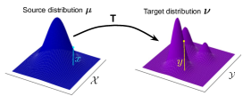
Figure 1: Conceptual illustration of optimal transport theory. Here, $\mu(x)$ is a probability distribution over the source space $\mathcal{X}$, and $\nu(y)$ is a probability distribution over the target space $\mathcal{Y}$. The arrows represent the optimal transport plan $T$, which reallocates mass from $\mu$ to $\nu$ to minimize the total transport cost.

Building on these strategies, we explore the use of optimal transport (OT) theory to enhance safety in RL by guiding the agent to prioritize visiting safer states during training. OT is highly valued for its ability to measure and optimize the alignment between probability distributions by minimizing the cost of transforming one distribution into another as shown in Fig. 1. It takes into account the geometry of the distributions and provides a more interpretable comparison, particularly when the distributions have non-overlapping supports or complex structures [14]. There are a few applications of OT in safe RL [15, 16, 17, 18, 19, 20]. For example, [16] apply OT theory to develop a safe RL framework that incorporates robustness through an OT cost uncertainty set. This approach constructs worst-case virtual state transitions using OT perturbations which improves safety in continuous control tasks compared to standard safe RL methods. [17] propose a novel approach called Wasserstein Q-learning (WQL), which uses Bayesian posterior distributions and Wasserstein barycenters to model and propagate uncertainty in RL. Their method demonstrates improved exploration and faster learning in tabular domains compared to classic RL algorithms. They also show preliminary success in adapting WQL to deep architectures for Atari games. [18] use OT for reward shaping in Q-learning. Through minimization of the Wasserstein distance between the policy’s stationary distribution and a predefined risk distribution, the agent is encouraged the agent to visit safe states more frequently.

In this letter, we incorporate OT theory into temporal difference (TD) learning to enhance agent safety during learning. We propose a risk-averse TD framework that considers both the reward and the uncertainty associated with actions without relying on expert knowledge or predefined safety constraints. We use Wasserstein distance to quantify the total risk level at each state and prioritize the actions that contribute less to this risk. This encourages the agent to take safer actions more frequently and avoid higher-risk ones. In other words, the agent tries to take actions with more predictable outcomes and avoid those with highly variable or uncertain consequences.

The contributions of this letter are: (i) introduction of a risk-averse TD learning algorithm to enhance agent safety, (ii) safety bounds of the algorithm which demonstrates less visitation to risky states, and (iii) applications on case studies with different forms of uncertainty in reward function, transition function, and states to show our algorithm reduces visiting unsafe states while preserving performance.

II Preliminaries

This section reviews Markov decision processes, partially observable Markov decision processes, temporal difference learning algorithms, and the basic principles of OT theory.

II-A Markov Decision Processes and Temporal Difference Learning

Markov Decision Processes (MDPs). MDPs represent a fully observable reinforcement learning environment. A finite MDP is defined by the tuple $\mathcal{M}=(\mathcal{S},\mathcal{A},\mathcal{T},\mathcal{R},\gamma)$, where $\mathcal{S}$ is a set of states, $\mathcal{A}$ is a set of actions, $\mathcal{T}:\mathcal{S}\times\mathcal{A}\times\mathcal{S}\to[0,1]$ is the transition probability function, where $\mathcal{T}(s^{\prime}|s,a)$ represents the probability of transitioning to state $s^{\prime}$ when action $a$ is taken in state $s$, $\mathcal{R}:\mathcal{S}\times\mathcal{A}\to\mathbb{R}$ is the reward function, and $\gamma\in[0,1)$ is the discount factor. The agent follows a policy $\pi:\mathcal{S}\times\mathcal{A}\rightarrow[0,1]$ that maps states to action probabilities, with the objective to maximize the expected discounted return, $G_{t}=\sum_{k=0}^{\infty}\gamma^{k}r_{t+k+1}$.

Temporal Difference Learning. The Q-value of action $a$ in state $s$ under policy $\pi$ is given by $Q_{\pi}(s,a)=\mathbb{E}_{\pi}[G_{t}|s_{t}=s,a_{t}=a]$, which can be incrementally learned. In one-step TD, the Q-value update rule is $Q(s_{t},a_{t})\leftarrow Q(s_{t},a_{t})+\alpha\delta_{t}$ where $\delta_{t}$ is the TD error at time $t$ and $\alpha$ is the learning rate. In the Q-learning algorithm [21], the TD error is defined as:

$$\delta_{t}=r_{t+1}+\gamma\max_{a}Q(s_{t+1},a)-Q(s_{t},a_{t})$$ (1)

Similarly, in the SARSA algorithm [22], the TD error is given by:

$$\delta_{t}=r_{t+1}+\gamma Q(s_{t+1},a_{t+1})-Q(s_{t},a_{t})$$ (2)

SARSA($\lambda$) extends one-step SARSA using eligibility traces to incorporate multi-step updates and improve learning efficiency. An eligibility trace tracks the degree to which each state-action pair has been recently visited, which enables updates to consider a weighted history of past experiences. The Q-value update rule in SARSA($\lambda$) is:

$$Q_{t+1}(s,a)=Q_{t}(s,a)+\alpha\delta_{t}e_{t}(s,a),\quad\text{for all }s,a$$ (3)

where $e_{t}(s,a)$ is the eligibility trace. The eligibility trace $e_{t}(s,a)$ decays over time and is updated as follows:

$$e_{t}(s,a)=\begin{cases}\gamma\lambda e_{t-1}(s,a)+1&\text{if }s=s_{t}\text{ and }a=a_{t}\\ \gamma\lambda e_{t-1}(s,a)&\text{otherwise}\end{cases}$$ (4)

where $\lambda\in[0,1]$ controls the trace decay rate. Higher $\lambda$ values give greater weight to longer-term past states. TD algorithms often use an $\epsilon$-greedy strategy for action generation. The parameter $\epsilon$ can either be fixed or decay over time to balance exploration and exploitation. The behavioral policy is expressed as:

$$\pi(s_{t},a_{t})=\begin{cases}1-\epsilon&\text{if }a_{t}\in\arg\max_{a}Q(s_{t},a)\\ \frac{\epsilon}{|\mathcal{A}|}&\text{otherwise}\end{cases}$$ (5)

Partially Observable MDPs (POMDPs). POMDPs generalize MDPs to account for environments where the agent cannot directly observe the underlying state. A POMDP is defined by the tuple $\mathcal{PM}=(\mathcal{S},\mathcal{A},\mathcal{O},\mathcal{T},\mathcal{R},\mathcal{Z},\gamma)$, where $\mathcal{S}$, $\mathcal{A}$, $\mathcal{T}$, $\mathcal{R}$, and $\gamma$ maintain their definitions from MDPs, and $\mathcal{O}$ is a set of observations the agent can perceive. The observation function $\mathcal{Z}:\mathcal{S}\times\mathcal{A}\to\mathcal{O}$ maps states and actions to observation probabilities.

II-B Optimal transport theory

The OT theory aims to find minimal-cost transport plans to move one probability distribution to another within a metric space. This involves a cost function $c(x,y)$ and two probability distributions, $\mu(x)$ and $\nu(y)$. The goal is to find a transport plan that minimizes the cost of moving $\mu$ to $\nu$ under $c(x,y)$, often using the Euclidean distance for explicit solutions [23].

We focus on discrete OT theory, assuming $\mu$ and $\nu$ as source and target distributions, respectively, both belonging to $\mathcal{P}p(\mathbb{R}^{n})$ with finite supports $\{x_{i}\}_{i=1}^{m_{1}}$ and $\{y_{j}\}_{j=1}^{m_{2}}$, and corresponding probability masses $\{a_{i}\}_{i=1}^{m_{1}}$ and $\{b_{j}\}_{j=1}^{m_{2}}$. The cost between support points is represented by an $m_{1}\times m_{2}$ matrix $C$, where $C_{ij}=|x_{i}-y_{j}|_{p}^{p}$ denotes the transport cost from $x_{i}$ to $y_{j}$. The OT problem seeks the transport plan $P^{\ast}$ that minimizes the cost while ensuring that the marginals of $P^{\ast}$ match $\mu$ and $\nu$:

$$\min_{P\in\mathbb{R}^{m_{1}\times m_{2}}}\sum_{i=1}^{m_{1}}\sum_{j=1}^{m_{2}}P_{ij}C_{ij}$$ (6)

Here, the coupling matrix $P_{ij}$ indicates the probability mass transported from $x_{i}$ to $y_{j}$ and $\sum_{j=1}^{m_{2}}P_{ij}=a_{i}$ for all $i$, and $\sum_{i=1}^{m_{1}}P_{ij}=b_{j}$ for all $j$. Additionally, $P_{ij}\geq 0$ for all $i,j$.

Definition 1 [23]: The Wasserstein distance between $\mu$ and $\nu$ is computed using the OT plan $P^{\ast}$ obtained from solving the above linear programming problem:

$$W_{p}(\mu,\nu)=\left(\langle P^{\ast},C\rangle\right)^{\frac{1}{p}}$$ (7)

where $p\geq 1$ and $\langle\cdot,\cdot\rangle$ denotes the inner product.

To enhance numerical stability and computational efficiency, an entropy regularization term can be added to the objective, leading to the regularized Wasserstein distance, which can be solved iteratively using the Sinkhorn iterations [24].

Definition 2 [24]: The Entropy-regularized OT problem is formulated as:

$$\min_{P\in\mathbb{R}^{m_{1}\times m_{2}}}\quad\sum_{i=1}^{m_{1}}\sum_{j=1}^{m_{2}}P_{ij}C_{ij}+\varepsilon\sum_{i=1}^{m_{1}}\sum_{j=1}^{m_{2}}P_{ij}(\log P_{ij}-1)$$ (8)

where $\varepsilon>0$ is a regularization parameter that balances transport cost and the entropy of the transport plan $P$.

III Methodology

Consider an RL agent interacting with an environment defined by an MDP. For each state $s$, we define the Q-distribution $Q_{s}$ as the normalized distribution over the agent’s estimated Q-values for the available actions $a_{i}$, $i=1,\ldots,N$. Formally, we have $Q_{s}=\sum_{i=1}^{N}q_{i}^{s}\delta_{\mathbf{a}_{i}}$, where $q_{i}^{s}$ is the probability assigned to action $a_{i}$ based on the current Q-value estimations, and $\delta_{\mathbf{a}_{i}^{s}}$ is the Dirac measure centered at $a_{i}$. Intuitively, $Q_{s}$ captures how the agent’s Q-values are distributed across actions at state $s$. We also introduce a corresponding T-distribution $T_{t}$, which represents a normalized distribution over the target values for the same set of actions. Specifically, we have $\quad T_{t}=\sum_{i=1}^{N}p_{i}^{t}\delta_{\mathbf{a}_{i}}$, where $p_{i}^{t}$ is the probability associated with action $a_{i}$ based on target values. For each action $a$ in state $s$, we define a risk indicator $U(s,a)$. The goal is to quantify how much an action contributes to the overall risk of the agent’s policy in that state. First, we compute the OT map $P^{\ast}$ between the Q-distribution $Q_{s}$ and the T-distribution $T_{t}$ by solving the entropy-regularized Wasserstein distance formulation. The total risk in state $s$ is measured by the Wasserstein distance $W(Q_{s},T_{t})$. For an action $a_{i}$, the flow $\Delta(s,a_{i})$ is defined as the absolute difference between the outgoing flow (transport from $a_{i}$ to other actions $b\neq a_{i}$) and the incoming flow (transport from other actions $b\neq a_{i}$ to $a_{i}$):

$$\Delta(s,a_{i})=\left|\sum_{b\neq a_{i}}P^{\ast}_{a_{i},b}-\sum_{b\neq a_{i}}P^{\ast}_{b,a_{i}}\right|$$ (9)

Here, the first summation $\sum_{b\neq a_{i}}P^{\ast}_{a_{i},b}$ represents how much probability mass is transported away from $a_{i}$ to other actions, while the second summation $\sum_{b\neq a_{i}}P^{\ast}_{b,a_{i}}$ denotes how much mass flows into $a_{i}$ from other actions. The absolute difference between these two flows, $\Delta(s,a_{i})$, captures how much the probability of an action in Q-distribution must be “redistributed” to match T-distribution. We subsequently normalize this value by the total Wasserstein distance:

$$U(s,a_{i})=\frac{\Delta(s,a_{i})}{W(Q_{s},T_{t})}$$ (10)

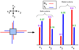
Figure 2: Example: For a fixed state and four available actions, we compute the total uncertainty of the state $W(Q_{s},T_{t})$ and the contribution of each action to this uncertainty.

TABLE I: Example: Incorporating uncertainty to the behavioral policy considering $\beta=0.5$. Standard SARSA chooses $a_{4}$, while our algorithm prefers $a_{2}$. The safest available action is $a_{1}$.

Action	$Q(s,a)$	$U(s,a)$	$Q(s,a)-\beta U(s,a)$
$a_{1}$	$0.2$	yellow$0.21$	$0.09$
$a_{2}$	$0.3$	$0.37$	yellow$0.112$
$a_{3}$	$0.1$	$0.78$	$-0.29$
$a_{4}$	yellow$0.4$	$0.62$	$0.087$

The risk indicator $U(s,a_{i})$ thus reflects how much action $a_{i}$ is responsible for the mismatch between $Q_{s}$ and $T_{t}$. Equivalently, it reveals to what extent the action $a_{i}$ needs to be adjusted (positively or negatively) for $Q_{s}$ to align with $T_{t}$ in a cost-efficient manner. Higher values of $\Delta(s,a_{i})$ indicate larger corrections to the probability of $a_{i}$ in $Q_{s}$, which suggest more uncertainty or risk. While standard SARSA does not account for safety, we incorporate the above risk indicator into the behavioral policy. Let $\beta$ be a risk sensitivity coefficient that specifies how strongly the agent prioritizes safety relative to reward. We then modify the behavioral policy as follows:

$$Q(s,a)-\beta U(s,a)$$ (11)

Importantly, the agent’s action-selection process is biased to favor actions with both high Q-values and low-risk indicators. Indeed, we encourage the agent to choose the action for which it has the highest confidence in the outcome among the actions experienced in that state. This approach enables a directed exploration strategy that prioritizes safer actions with higher rewards. Notably, the uncertainty we address here is aleatoric, which is inherent to the environment and irreducible. Example $1$ further illustrates the influence of this risk indicator on both Q-values and policy decisions. In particular, it demonstrates the trade-off between exploiting high-return actions and mitigating high-risk actions to ensure safer exploration and more stable learning.

In the context of POMDPs, we use the SARSA($\lambda$) variant. Specifically, the Q and target distributions associated with the agent’s current observation $o$ and the available actions $a_{1},\cdots,a_{N}$ are integrated into the safety indicator term $U(o,a_{i})$. Moreover, the flexibility of our approach enables its extension to scenarios that involve using multiple consecutive observations $o_{t-n},\cdots,o_{t}$, which can help the algorithm better capture non-Markovian properties.

Example: Consider a fixed state $s$ with four available actions. For this state, we have access to Q- and T-distributions over actions as depicted in Fig. 2. Table. I shows that how the risk indicator term affects the Q-values and action selection. As observed, $a_{1}$ is the safest action and $a_{4}$ offers the highest reward. In decision-making, standard SARSA prefers action $a_{4}$, whereas risk-averse SARSA chooses $a_{2}$ to balance the reward and safety.

Theorem 1

Let $\mathcal{S}_{\text{risk }}\subset\mathcal{S}$ be a set of hazardous or “risky” states to avoid. For each $t$, define policy $\pi_{t}$ to be the $\epsilon$-greedy policy derived from the risk-augmented Q -values $Q_{t}(s,a)-\beta U_{t}(s,a)$. Assume that every state-action pair is explored infinitely often in the limit (i.e., persistent exploration) and the step-size $\left\{\alpha_{t}\right\}$ satisfies usual stochastic-approximation conditions. Then for sufficiently large $\beta$, there exists a constant $0<c<1$ such that

$$\lim_{t\rightarrow\infty}\operatorname{Pr}_{\pi_{t}}\left[s\in\mathcal{S}_{\text{risk }}\right]\leq c\cdot\operatorname{Pr}_{\pi^{0}}\left[s\in\mathcal{S}_{\text{risk }}\right],$$ (12)

where $\pi^{0}$ is a baseline policy (e.g., standard SARSA’s $\epsilon$-greedy policy w.r.t. $Q$ alone).

Proof:

Let $\mathcal{M}=(\mathcal{S},\mathcal{A},\mathcal{T},\mathcal{R},\gamma)$ be a finite MDP with state space $\mathcal{S}$ and action space $\mathcal{A}$. Any stationary policy $\pi:\mathcal{S}\rightarrow\mathcal{P}(\mathcal{A})$ (where $\mathcal{P}(\mathcal{A})$ is the space of distributions over actions) induces a transition probability

$$P_{\pi}\left(s^{\prime}\mid s\right)=\sum_{a\in\mathcal{A}}\pi(a\mid s)\mathcal{T}\left(s^{\prime}\mid s,a\right)$$ (13)

Because the state and action sets are finite, each $\pi$ yields a finite-state Markov chain with transition matrix $P_{\pi}$. If $P_{\pi}$ is irreducible and aperiodic, there is a unique stationary distribution $\mu_{\pi}$. By the Ergodic Theorem for Markov chains, for any initial state $s_{0}$, the fraction of time the chain spends in state $s$ converges to $\mu_{\pi}(s)$ almost surely. Suppose $\pi^{0}$ is derived from (say) standard SARSA or Q-learning with $\epsilon$-greedy action selection based purely on $Q(s,a)$. Let $\mu^{0}$ be the unique stationary distribution of the Markov chain induced by $\pi^{0}$. Then

$$\underset{\pi^{0}}{\operatorname{Pr}}\left\{s\in\mathcal{S}_{\text{risk }}\right\}=\sum_{s\in\mathcal{S}_{\text{rikk }}}\mu^{0}(s)$$ (14)

In contrast, the “safe” policy $\pi_{t}$ at episode (or time) $t$ follows an $\epsilon$-greedy strategy with respect to the risk-adjusted Q-values, $Q_{t}(s,a)-$ $\beta U_{t}(s,a)$

$$\pi_{t}(a\mid s)=\begin{cases}1-\epsilon,&\text{if }a\in\arg\max\limits_{a^{\prime}}\big{(}Q_{t}(s,a^{\prime})-\beta U_{t}(s,a^{\prime})\big{)}\\[6.0pt] \frac{\epsilon}{|\mathcal{A}|},&\text{otherwise.}\end{cases}$$ (15)

For large $\beta$, actions with large $U_{t}(s,a)$ become less likely to be chosen. Over time $t\rightarrow\infty$, if the algorithm converges, then $Q_{t}\rightarrow Q_{\beta}^{*}$ and $U_{t}\rightarrow U_{\beta}^{*}$ in some stable sense, and hence $\pi_{t}\rightarrow\pi_{\beta}$. Let $\pi_{\beta}$ denote the limiting “risk-averse” policy and $\mu_{\beta}$ its stationary distribution. Intuitively, if an action $a$ leads frequently to or transitions inside $\mathcal{S}_{\text{risk }}$, it will accumulate a larger risk indicator $U(s,a)$, because repeatedly visiting or transitioning into hazardous states forces significant “corrections” in the Q-distribution (cf. the definition of $U$ via OT). Under the update $Q(s,a)-\beta U(s,a)$, if $U(s,a)$ is large, then $Q(s,a)-\beta U(s,a)$ might be substantially less than competing actions. Thus, for large $\beta$, the probability $\pi_{\beta}(a\mid s)$ of choosing such a risky action decreases, unless its Q-value is significantly higher than the alternatives. We now compare $\mu_{\beta}\left(\mathcal{S}_{\text{risk }}\right)$ (the stationary measure of risky states under $\left.\pi_{\beta}\right)$ with $\mu^{0}\left(\mathcal{S}_{\text{risk }}\right)$ (the stationary measure under $\pi^{0}$). Let $\mathcal{A}_{\text{risk }}(s)\subseteq\mathcal{A}$ denote the actions in state $s$ whose transitions have high probability of landing in $\mathcal{S}_{\text{risk }}$ or staying there. Formally, for a given threshold $\delta>0$, define

$$\mathcal{A}_{\text{risk }}(s)=\left\{a\in\mathcal{A}:\operatorname{Pr}\left[s_{t+1}\in\mathcal{S}_{\text{risk }}\mid s_{t}=s,a_{t}=a\right]\geq\delta\right\}$$ (16)

Because $\beta U(s,a)$ increases if an action is repeatedly leading to these hazardous states, for $\beta$ sufficiently large, actions in $\mathcal{A}_{\text{risk }}(s)$ are given low preference in $\pi_{\beta}$. One classical method is to compare two Markov chains $P_{\pi^{0}}$ and $P_{\pi_{\beta}}$ via a coupling argument. Intuitively, whenever $\pi^{0}$ chooses a “risky” action in state $s,\pi_{\beta}$ might choose a safer action in the same state with strictly higher probability if $\beta$ is large. Over many transitions, the chain under $\pi_{\beta}$ accumulates strictly fewer visits to $\mathcal{S}_{\text{risk }}$. In finite-state Markov chains, the stationary distribution $\mu$ is the normalized left-eigenvector of the transition matrix $P$. As we tune $\beta\rightarrow\infty$, the transition probabilities in $P_{\pi_{\beta}}\left(s^{\prime}\mid s\right)$ that lead to $\mathcal{S}_{\text{risk }}$ shrink, while transitions within the safe region $\mathcal{S}\backslash\mathcal{S}_{\text{risk }}$ become more likely. Consequently, the fraction of time spent in $\mathcal{S}_{\text{risk }}$ must decrease compared to the baseline. Formally,

$$\mu_{\beta}(s)=\frac{1}{Z_{\beta}}\exp(\Phi(s,\beta))\mu^{0}(s)$$ (17)

for some function $\Phi$ that accounts for changes in transition probabilities. Because transitions to $\mathcal{S}_{\text{risk }}$ are heavily penalized for large $\beta,\Phi$ is negative for $s\in\mathcal{S}_{\text{risk }}$; thus $\mu_{\beta}\left(\mathcal{S}_{\text{risk }}\right)$ must shrink relative to $\mu^{0}\left(\mathcal{S}_{\text{risk }}\right)$. Since the long-run fraction of time spent in $\mathcal{S}_{\text{risk }}$ converges to the respective stationary measure for each chain, we obtain

$$\begin{split}\lim_{t\rightarrow\infty}\operatorname{Pr}\left\{s\in\mathcal{S}_{\text{risk }}\right\}&=\mu_{\beta}\left(\mathcal{S}_{\text{risk }}\right)\\ &\leq c\mu^{0}\left(\mathcal{S}_{\text{risk }}\right)=c\underset{\pi^{0}}{\operatorname{Pr}}\left\{s\in\mathcal{S}_{\text{risk }}\right\}.\end{split}$$ (18)

∎

IV Experimental Results

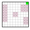
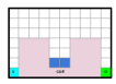
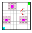
Figure 3: Case studies with low uncertainty level: (Left) grid-world with slippery states, (Center) cliff walking with traps, where the blue cells represent the trap region. (Right) rover navigation task with partial observability of obstacle locations.

IV-A Case Studies

We evaluate risk-averse SARSA in three case studies with uncertainties in rewards, transitions, and states (Fig. 3). For each case, we conduct experiments under low and high uncertainty levels and further examine the effect of increasing the environment size on performance.

Case study 1: Grid-world with Reward Uncertainty. We consider a $10\times 10$ grid-world environment with normal, goal, and slippery states [12]. The agent can move up, down, left, and right. For any movement to a normal state, the agent receives the reward of $-1$, while transitions to slippery states result in a random reward in the range $[-12,10]$. Collisions with walls incur a reward of $-10$. The episode terminates when the agent either reaches the goal state in the top-right corner or completes a maximum of $100$ steps.

Case study 2: Cliff Walking with Transition Uncertainty. The cliff walking environment [25] consists of three zones: the cliff region, the trap region, and the feasible region. The agent starts at the bottom-left corner to reach the goal at the bottom-right corner while avoiding the cliff zone, which represents unsafe states. Entering the cliff region results in task failure. The agent can move freely within the feasible region in four directions: up, down, left, and right. Entering the trap region forces the agent to move downward, regardless of its chosen action, eventually ending up in the cliff region. Each movement yields a reward of $-1$. If the agent collides with the environment borders, its position remains unchanged, but it still earns the movement reward. Reaching the target earns the agent a reward of $101$, while entering the cliff region results in a $-49$ penalty.

TABLE II: Average R $\pm$ Std over different algorithms on grid-world environment.

Scenario	SARSA	Q-learning	Ours
$10\times 10$ LU	$-15.70\pm 17.32$	$-13.38\pm 14.53$	yellow$-12.04\pm 12.83$
$10\times 10$ HU	$-16.26\pm 20.38$	$-14.14\pm 18.52$	yellow$-12.92\pm 16.79$
$30\times 30$ HU	$-119.16\pm 126.65$	$-108.21\pm 118.76$	yellow$-98.77\pm 112.15$

Case study 3: Rover Navigation with Partial Observability. In this case study, a rover must navigate a two-dimensional terrain map represented as a $10\times 10$ grid, where $3$ of the grid cells are obstacles. Each grid cell represents a state, and the rover can move in eight geographic directions. However, the environment is stochastic; for example, as shown in Fig. 3, when the rover takes the action east, it moves to the intended grid cell with a probability of $0.9$ but may move to one of the adjacent cells with a probability of $0.05$. Partial observability exists because the rover cannot directly detect the locations of obstacle cells through its measurements. When the rover moves to a cell adjacent to an obstacle, it can identify the exact location of the obstacle (marked in magenta) with a probability of $0.6$ and observe a probability distribution over nearby cells (marked in pink). Colliding with an obstacle results in an immediate penalty of $10$, while reaching the goal region provides no immediate reward. All other grid cells impose a penalty of $2$. We consider $\gamma=0.99$ and $\lambda=0.9$.

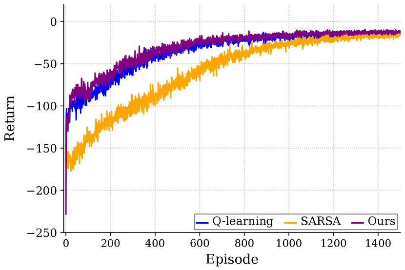
(a)

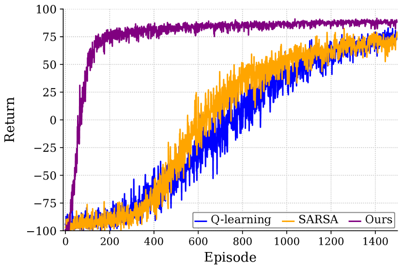
(b)

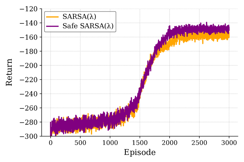
(c)

Figure 4: Comparison between average cumulative reward over $50$ random seeds for (a) grid-world and (b) cliff walking (c) rover navigation case studies with low uncertainty level. In all case studies, risk-averse SARSA outperforms other baselines.

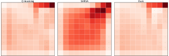
Figure 5: Comparison between state visitation density for different algorithms on grid-world with low uncertainty.

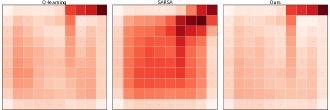
Figure 6: Comparison between state visitation density for different algorithms on grid-world with high uncertainty.

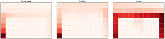
Figure 7: Comparison between the density of state visitation for different algorithms in case of cliff walking low uncertainty.

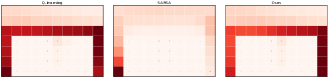
Figure 8: Comparison between the density of state visitation for different algorithms in case of cliff walking high uncertainty.

IV-B Discussion

Fig. 4 shows the average return of different algorithms over $50$ random seeds for different case studies with a low level of uncertainty. The results demonstrate that the risk-averse SARSA algorithm converges to a higher return value and exhibits higher stability throughout the learning process, mainly because of the risk indicator term, which guides exploration toward safer and more consistent actions. For the cliff walking case study, risk-averse SARSA not only achieves rapid convergence but also demonstrates a higher confidence in its return estimates. In contrast, both Q-learning and SARSA display greater variability, which reflects higher uncertainty in their returns.

Scenario	R/F	SARSA	Q-Learning	Ours
$10\times 7$ LU	R $\pm$ Std	$72.48\pm 36.1$	$74.59\pm 28.52$	yellow$87.99\pm 10.65$
	F	$72.74$	$61.46$	yellow$21.74$
$10\times 7$ HU	R $\pm$ Std	$69.82\pm 38.69$	$84.27\pm 23.99$	yellow$89.53\pm 8.65$
	F	$196.94$	$77.56$	yellow$30.14$
$30\times 21$ HU	R $\pm$ Std	$-177.07\pm 54.61$	$42.11\pm 37.44$	yellow$55.59\pm 22.36$
	F	$523.64$	$362.66$	yellow$196.48$

TABLE III: Average performance metrics for different scenarios of cliff walking environment.

Table. II, III, and IV present a quantitative comparison of risk-averse SARSA performance to other baselines, providing the average return (R) and standard deviation (std) under low uncertainty (LU), high uncertainty (HU), and increasing environment size scenarios across last $20$ episodes for all case studies. The results in Table. II confirm that risk-averse SARSA achieves the highest return and the lowest std in different scenarios. We present the state visitation map for LU and HU shown in Fig. 5 and Fig. 6. As expected, the SARSA algorithm, which lacks any safety considerations, demonstrates a high frequency of visits to slippery regions (darker red). In contrast, Q-learning performs better by exploring more efficient paths, but it still exhibits notable visits to unsafe states in comparison to risk-averse SARSA. For the cliff walking case study, the observations in Table. III demonstrate that risk-averse SARSA outperforms SARSA and Q-learning algorithms by converging to higher return values with lower std values. For this case study, the state visitation graph in Fig. 7 and Fig. 8 highlights the limitations of SARSA, where the agent struggles to identify the optimal path to the goal state in both LU and HU scenarios. Consequently, most episodes end without successfully reaching the goal. Q-learning performance is closer to our algorithm, however the rate of reaching the goal and escaping from the cliff at the beginning of episodes is lower than risk-averse SARSA. Moreover, in this case study number of failures (F) for risk-averse agent is significantly lower than both SARSA and Q-learning. For instance, in the LU scenario, risk-averse SARSA reduces failures by $35\%$ compared to SARSA and $30\%$ compared to Q-learning. This reduction is even greater in the other two scenarios. Overall, in both MDP case studies, our algorithm obtained a higher cumulative reward than Q-learning and SARSA, while improving the stability and the safety of the agent by avoiding unpredictable actions. Furthermore, for both MDP case studies, although increasing the size of the environment causes lower return values, risk-averse SARSA still maintains the best performance.

Scenario	R/F	SARSA($\lambda$)	Ours
$10\times 10$ LU	R $\pm$ Std	$-155.04\pm 109.09$	yellow$-149.96\pm 106.41$
	F	$2805.73$	yellow$2663.48$
$10\times 10$ HU	R $\pm$ Std	yellow$-247.70\pm 102.58$	$-264.00\pm 89.72$
	F	$9039.29$	yellow$8948.18$
$30\times 30$ HU	R $\pm$ Std	yellow$-1020.70\pm 39.26$	$-1024.74\pm 57.09$
	F	$30026.71$	yellow$30026.71$

TABLE IV: Average number of obstacle collisions for SARSA($\lambda$), and risk-averse SARSA($\lambda$) algorithms for POMDP case study.

For the POMDP case study, as can be seen in Table. IV, risk-averse SARSA($\lambda$) achieves superior performance compared to standard SARSA($\lambda$) in the case of low-partial observability. By increasing the partial observability degree (HU) and the size of the environment, the agent performance falls back. This shows that the performance of our algorithm can be influenced by the degree of partial observability in the environment. Specifically, when the agent receives indistinguishable or highly similar observations for different underlying states, the accuracy of the estimated Q-value and target distributions and, consequently, the reliability of the risk indicator becomes questionable. The number of failures for risk-averse SARSA($\lambda$) across the three scenarios is slightly lower than SARSA($\lambda$).

V Conclusions

We presented a risk-averse temporal difference algorithm based on optimal transport theory. We demonstrated the effectiveness of this approach in encouraging agents to prioritize less uncertain actions, leading to a reduction in visits to risky states and an improvement in cumulative rewards. Compared to standard temporal difference algorithms, our algorithm demonstrated robust performance in environments with reward, transition, and state uncertainties. Although our algorithm outperforms standard TD learning methods, it has its limitations. Determining the optimal transport map for candidate actions at each state is computationally expensive. While using the entropy-regularized extension of OT reduces this computational cost, further improvements in computational efficiency will be a focus of future work.

References

- [1] Shangding Gu, Long Yang, Yali Du, Guang Chen, Florian Walter, Jun Wang and Alois Knoll “A review of safe reinforcement learning: Methods, theories and applications” In IEEE Transactions on Pattern Analysis and Machine Intelligence IEEE, 2024
- [2] Javier Garcıa and Fernando Fernández “A comprehensive survey on safe reinforcement learning” In Journal of Machine Learning Research 16.1, 2015, pp. 1437–1480
- [3] Matthias Heger “Consideration of risk in reinforcement learning” In Machine Learning Proceedings Elsevier, 1994, pp. 105–111
- [4] Chris Gaskett “Reinforcement learning under circumstances beyond its control” In International Conference on Computational Intelligence for Modelling Control and Automation, 2003
- [5] Makoto Sato, Hajime Kimura and Shibenobu Kobayashi “TD algorithm for the variance of return and mean-variance reinforcement learning” In Transactions of the Japanese Society for Artificial Intelligence 16.3 Japanese Society for Artificial Intelligence, 2001, pp. 353–362
- [6] Peter Geibel and Fritz Wysotzki “Risk-sensitive reinforcement learning applied to control under constraints” In Journal of Artificial Intelligence Research 24, 2005, pp. 81–108
- [7] Joshua Achiam, David Held, Aviv Tamar and Pieter Abbeel “Constrained policy optimization” In International Conference on Machine Learning, 2017, pp. 22–31 PMLR
- [8] Yinlam Chow, Ofir Nachum, Aleksandra Faust, Edgar Duenez-Guzman and Mohammad Ghavamzadeh “Lyapunov-based safe policy optimization for continuous control” In arXiv preprint arXiv:1901.10031, 2019
- [9] Ali Baheri, Subramanya Nageshrao, H Eric Tseng, Ilya Kolmanovsky, Anouck Girard and Dimitar Filev “Deep reinforcement learning with enhanced safety for autonomous highway driving” In IEEE Intelligent Vehicles Symposium (IV), 2020, pp. 1550–1555
- [10] Yoshihiro Okawa, Tomotake Sasaki, Hitoshi Yanami and Toru Namerikawa “Safe exploration method for reinforcement learning under existence of disturbance” In Joint European Conference on Machine Learning and Knowledge Discovery in Databases, 2022, pp. 132–147 Springer
- [11] Jorge Ramirez and Wen Yu “Safe Reinforcement Learning for Learning from Human Demonstrations”, 2023
- [12] Clement Gehring and Doina Precup “Smart exploration in reinforcement learning using absolute temporal difference errors” In International Conference on Autonomous Agents and Multi-agent Systems, 2013, pp. 1037–1044
- [13] Edith LM Law “Risk-directed exploration in reinforcement learning” In PhD thesis McGill University, 2005
- [14] Filippo Santambrogio “Optimal transport for applied mathematicians” In Birkäuser, NY 55.58-63 Springer, 2015, pp. 94
- [15] Ali Baheri “Risk-aware reinforcement learning through optimal transport theory” In arXiv preprint arXiv:2309.06239, 2023
- [16] James Queeney, Erhan Can Ozcan, Ioannis Ch Paschalidis and Christos G Cassandras “Optimal transport perturbations for safe reinforcement learning with robustness guarantees” In arXiv preprint arXiv:2301.13375, 2023
- [17] Alberto Maria Metelli, Amarildo Likmeta and Marcello Restelli “Propagating uncertainty in reinforcement learning via Wasserstein barycenters” In Advances in Neural Information Processing Systems 32, 2019
- [18] Zahra Shahrooei and Ali Baheri “Optimal Transport-Assisted Risk-Sensitive Q-Learning” In arXiv preprint arXiv:2406.11774, 2024
- [19] Ali Baheri “The Synergy Between Optimal Transport Theory and Multi-Agent Reinforcement Learning” In arXiv preprint arXiv:2401.10949, 2024
- [20] Ali Baheri “Understanding reward ambiguity through optimal transport theory in inverse reinforcement learning” In arXiv preprint arXiv:2310.12055, 2023
- [21] Christopher JCH Watkins and Peter Dayan “Q-learning” In Machine learning 8 Springer, 1992, pp. 279–292
- [22] Gavin A Rummery and Mahesan Niranjan “On-line Q-learning using connectionist systems” University of Cambridge, Department of Engineering Cambridge, UK, 1994
- [23] Cédric Villani “Optimal transport: old and new” Springer, 2009
- [24] Marco Cuturi “Sinkhorn distances: Lightspeed computation of optimal transport” In Advances in Neural Information Processing Systems 26, 2013
- [25] Chengbin Xuan, Feng Zhang and Hak-Keung Lam “SEM: Safe exploration mask for Q-learning” In Engineering Applications of Artificial Intelligence 111 Elsevier, 2022, pp. 104765