Optimality and Renormalization
imply Statistical Laws

Abstract

Benford’s Law is an important instance of experimental mathematics that appears to constrain the information–theoretic behavior of numbers. Elias’ encoding for integers is a remarkable approach to universality and optimality of codes. In the present analysis we seek to deduce a general law and its particular implications for these two cases from optimality and renormalization as applied to information–theoretical functionals. Both theoretical and experimental results corroborate our conclusions.

1 The Information Theory underlying Benford’s Law

1.1 A probabilistic model for binary numbers

Herein, we present a Maximum Entropy formulation of Benford’s Law. We shall assume that a large integer may be represented as an unbounded binary code of $0$s and $1$s which is limited by the introduction of a stop symbol $S$. We shall also observe a threshold phenomenon associated to Benford’s Law applicability to number so generated.

Let a binary string $\beta$ be produced by the following probabilistic program:

• $\beta=``0"$ with probability $p_{0}$, or $\beta=``1"$ with probability $p_{1}$, otherwise;

• For codes of length $\lvert\beta\rvert>1$, set $\beta=``1"\gamma$, where $\gamma$ is generated by spawning ’0’ with probability $p_{0}$, $``1"$ with probability $p_{1}$, and $S$ with probability $p_{S}$. The generation of $\gamma$ is abandoned if $S$ is obtained and $S$ is not explicitly included at the end of the code.

Here we assume that the event of spawning $``0"$, $``1"$ and $``S"$ are independent and the probabilities satisfy

$$p_{0}+p_{1}+p_{S}=1.$$ (1)

There are no additional assumptions besides the equality $p_{0}=p_{1}$ due to the apparent symmetry.

1.2 Large deviations

Given the above probabilistic program, any binary number with $k>1$ bits may be expressed as a code $\beta$ starting with $``1"$ and continued with $k$ random symbols until $S$ is generated. Thus, the probability of $\beta$ is given by the geometric distribution

$$P(k)=(1-p_{S})^{k-1}\cdot p_{S},$$ (2)

and the expected length of $\beta$ is given by

$$\mathbb{E}[|\beta|]=1+\mathbb{E}[k-1]=\mathbb{E}[k]=\frac{1}{p_{S}}.$$ (3)

The order of magnitude $\Omega(k)$ of a binary number with $k\geq 1$ bits is $2^{k-1}$, if we consider as such the largest value it may take. It follows that

$$\mathbb{E}[\Omega]=\sum_{k=1}^{\infty}\Omega(k)\cdot P(k)=p_{S}\cdot\sum_{k=0}^{\infty}2^{k}\cdot(1-p_{S})^{k}=\begin{cases}\frac{p_{S}}{2p_{S}-1},&\text{if $p_{S}>\frac{1}{2}$},\\ \infty,&\text{$p_{S}\leq\frac{1}{2}$}.\end{cases}$$ (4)

While $\mathbb{E}[\Omega]$ diverges due to large deviations, we may estimate the typical stopping time and hence the typical order of magnitude using the geometric mean:

$$\mathbb{E}[\log_{2}\Omega]=\mathbb{E}[|\beta|]-1\sim\frac{1}{p_{S}}.$$ (5)

It follows that the typical number $\beta$ is on the scale of

$$\chi=2^{\mathbb{E}[\log_{2}\Omega]}\sim 2^{\frac{1}{p_{S}}}.$$ (6)

which we call the characteristic scale.

1.3 From Maximum Entropy to Benford’s Law

Using the Principle of Maximum Entropy, we would like to constrain the model parameters so that the numbers are distributed approximately uniformly up to binary length $N$.

Hence, given the cumulative distribution function of $k=|\beta|-1$

$$F(k)=1-(1-p_{S})^{k},$$ (7)

we apply the constraint

$$F(k)\approx\frac{k}{N},$$ (8)

for $0\leq k\leq N$.

As we may only satisfy this constraint on average, we have

$$(1-p_{S})^{N}=\frac{1}{N}\sum_{k=1}^{N}(1-p_{S})^{N}=\frac{1}{N}\sum_{k=1}^{N}\big{(}1-\frac{k}{N}\big{)}^{N/k}\approx\int_{0}^{1}(1-u)^{\frac{1}{u}}du,$$ (9)

for large $N\gg 1$.

Now, we may define the auxiliary parameter

$$\lambda=\int_{0}^{1}(1-u)^{\frac{1}{u}}du\approx 0.23075...,$$ (10)

so that

$$p_{S}=1-\lambda^{1/N},$$ (11)

where $p_{S}\rightarrow 0$ as $N\to\infty$.

On the other hand, we find:

$$p_{0}=p_{1}=\frac{\lambda^{1/N}}{2}=p_{\lambda,N},$$ (12)

where $p_{\lambda,N}\rightarrow\frac{1}{2}$ as $N\to\infty$.

Finally, we may deduce the cumulative distribution

$$F(k)=1-\lambda^{k/N}\approx\frac{k}{N}\cdot\ln\frac{1}{\lambda}$$ (13)

using the first term in the expansion

$$x^{k/N}=\sum_{n=0}^{\infty}\frac{k^{n}(\frac{\ln x}{N})^{n}}{n!},$$ (14)

as higher order terms become negligible for $N\gg 1$.

Within each order of magnitude $k$ all strings have the same probability

$$p(k,\lambda,N)=p_{\lambda,N}^{k-1},$$ (15)

to be generated, and thus for any fixed $k$ the distribution is uniform.

Since

$$P(k)=F(k)-F(k-1)=\frac{1}{N}\cdot\ln\frac{1}{\lambda}$$ (16)

does not depend on $k$, the distribution is uniform (up to a multiple) throughout all orders of magnitude $1\leq k\leq N$.

In other words, if $X$ is generated by our model, then $\log_{2}(X)$ is distributed roughly uniformly. In fact, the order of magnitude $k=\lfloor\log_{2}(X)\rfloor$ is distributed uniformly because of (16), and within each order of magnitude $\{\log_{2}(X)\}$ tends to the uniform distribution because we have a large and large amount of numbers generated each with the same probability (15).

Then,

$$d\cdot 10^{m}\leq X<(d+1)\cdot 10^{m}$$ (17)

is equivalent to

$$\log_{2}d+m\cdot\log_{2}10\leq\log_{2}X<\log_{2}(d+1)+m\cdot\log_{2}10,$$ (18)

which, by the above reasoning, has probability proportional to the length of the interval:

$$P(d)\sim\log_{2}\left(1+\frac{1}{d}\right).$$ (19)

This is, after an appropriate normalization, equivalent to Benford’s Law. It is also important to point out that the arguments above are largely heuristic, and not entirely rigorous. However, our numerical experiments suggest that the model’s behavior is largely as expected.

2 Numerical experiments

We perform some experiments to support our conclusions: the corresponding Python code is available on Github [KR25]. First, we generate binary strings as prescribed by our model, convert them to decimals, and take the leading digit. In each case we generate $10000$ binary strings with $N=64$ (which is the largest binary length for Benford’s law to hold a priori, see Section 1.3) and $\lambda\in\{10^{-12},10^{-6},0.1,0.230759776818,$ $0.3,0.4,0.5,0.6,0.7,0.8,0.9\}$.

It turns out that

$$\lambda_{*}=\int^{1}_{0}(1-u)^{1/u}\,du\approx 0.230759776818\ldots$$

relates to a threshold effect, see Figure 1.

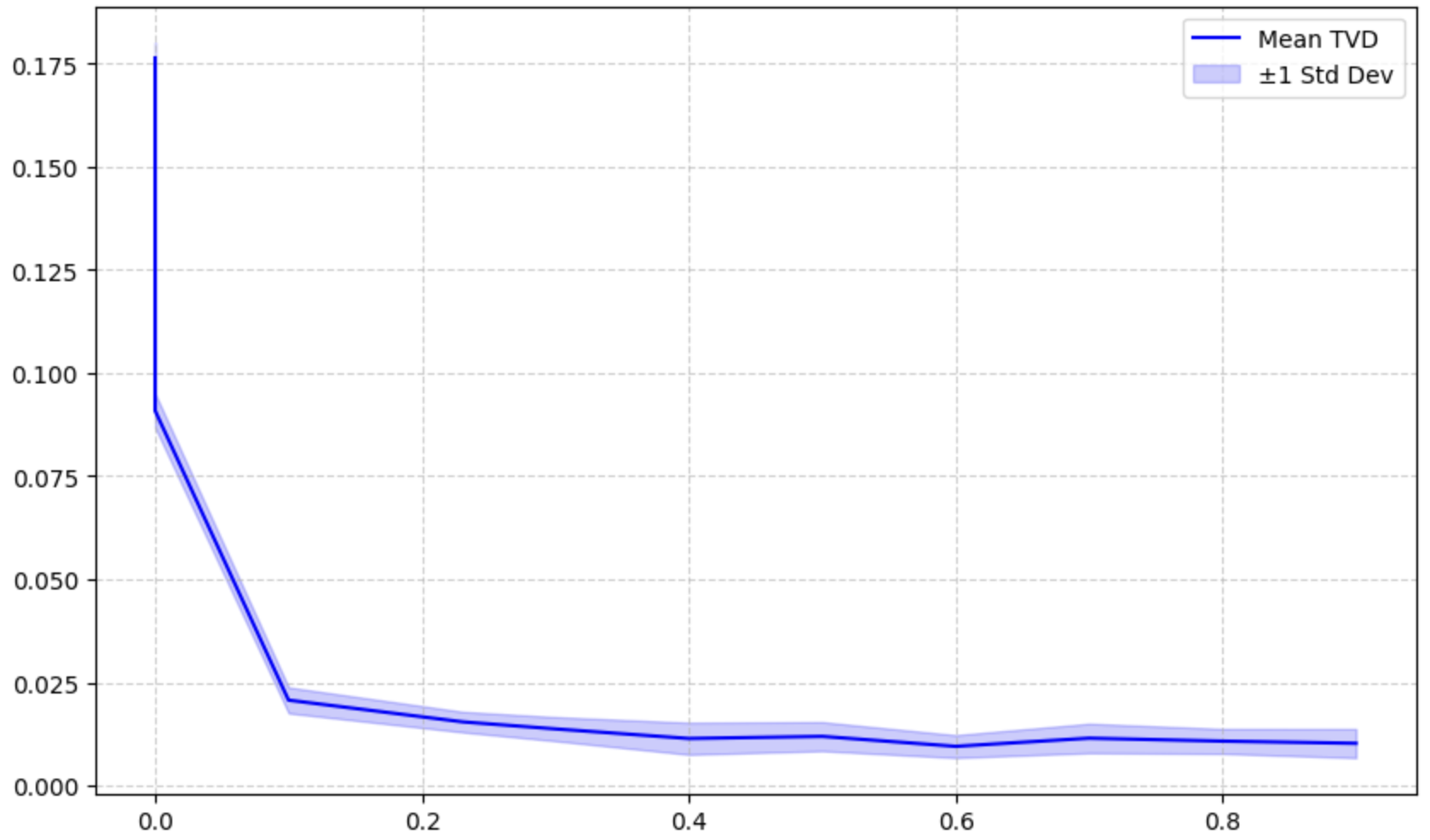
Figure 1: TVD from the model distribution of first significant digits to Benford’s law. The model parameter $\lambda$ responsible for the halting probability is on the horizontal axis: $\lambda=10^{-12},10^{-6},0.1,0.23076(\approx\lambda_{*}),$ $0.3,0.4,0.5,0.6,0.7,0.8,0.9$. Another parameter is set to $N=64$ throughout. The plateau starts at $\lambda=\lambda_{*}$.

Namely, for $\lambda<\lambda_{*}$ we do not observe that the numbers generated conform very strictly to Benford’s law (though they do compare to the real–life dataset we use. However, for $\lambda\geq\lambda_{*}$ we see that the total variation distance (TVD) drops down significantly (and apparently plateaus).

Second, we choose the dataset of city populations available from [Div24]. However, this dataset turns out not to follow Benford’s law very closely: the TVD between the empirical distribution and Benford’s law in this case is about $0.279507$.

The interesting observation is that were the dataset modeled by our approach, it would have halting probability $p_{S}=0.054689$, as the average binary length equals $18.285235$. The maximum binary length of the dataset is $N=25$.

If we use the ternary model with $p_{S}=0.054689$, we get a close average binary length, as expected. However, the maximum binary length is much larger $N>200$. In this case, the TVD between the model distribution and Benford’s law is about $0.02287$, which is a much closer match.

3 Non–ergodicity of large partitions

The following analysis is based off Oded Kafri’s statistical mechanical model for Benford’s Law, though it elucidates a diffeent aspect and also aims to correct some mathematical inconsistencies of the original argument provided in [Kaf09].

An $N$–digit number in base $\Omega\in\mathbb{N}$ may be modeled as a random vector with $N$ components where each component has value between $0$ and $\Omega-1$.

Let us consider the function $\phi(\sigma)$ that counts the number of components of $\vec{X}_{N}$ that equal $\sigma$. Also, we have

$$\frac{1}{N}\sum^{\Omega-1}_{\sigma=0}\phi(\sigma)=1,$$ (20)

which means that $\phi$ plays the role of a counting measure.

Let the “average digit” of $\vec{X}_{N}$ be

$$\mu=\frac{1}{N}\sum^{\Omega-1}_{i=0}\sigma\cdot\phi(\sigma).$$ (21)

Then, at time step $0\leq i\leq N$, we scale the average back by $i/N$ and get “on average” $\phi(i\cdot\mu/N)$ components. Here, $\phi$ should be understood as a distribution over the possible component values on a continuous rather than discrete range. This can be achieved by looking at $\phi$ as a generalized function, or an interpolant over a discrete set of values.

Then the time average of digits of $\vec{X}_{N}$ is

$$\frac{1}{N}\sum^{N}_{i=0}\mu\cdot\phi\left(\frac{i\cdot\mu}{N}\right)\rightarrow\int^{\mu}_{0}\phi(t)dt.$$ (22)

If we assume that $\vec{X}_{N}$ is generated in ergodic manner, then the spatial and temporal averages of our dynamical system would coincide. Setting the time average equal to the spatial average, as ergodicity would imply via Birkhoff’s theorem, results in the trivial solution $\phi(\mu)=1$. Thus, we must essentially employ the non–ergodicity of the process.

Let us constrain first the spatial entropy of our sequence:

$$\sum^{\Omega-1}_{i=0}\sigma\cdot\phi(\sigma)=\mu N=\mathcal{E}=const.$$ (23)

To estimate the number of vectors $\vec{X}_{N}$ with entropy constraint $\mathcal{E}$, it suffices to consider the combinatorial expression:

$$\Lambda(N,\mathcal{E})=\frac{(N+\mathcal{E}-1)!}{(N-1)!\mathcal{E}!}.$$ (24)

By using Stirling’s approximation, we find

$$\ln\Lambda\approx N\big{(}(1+\mu)\cdot\ln(1+\mu)-\mu\cdot\ln\mu\big{)}.$$ (25)

However, the temporal entropy should also be constrained in some way. Here, however, we posit that we can only constrain the time average of digits. This means that the entropy rate is limited: the generation of each next digit has bounded entropy, while the whole process is open–ended and unbounded in time.

Thus, we have

$$\int^{\mu}_{0}\phi(t)dt=\varepsilon=const.$$ (26)

Now, to find $\phi(\mu)$ that maximizes entropy we may specify a Lagrangian in terms of the entropy $\ln\Lambda(\mu)$ and the marginal entropy constraint $\mathcal{E}$:

$$\mathcal{L}(\mu)=\ln\Lambda-\beta\cdot\left(\int^{\mu}_{0}\phi(t)dt-\varepsilon\right).$$ (27)

By using (25) we find

$$\frac{\partial\mathcal{L}}{\partial\mu}=0\implies\phi(\mu)=\frac{N}{\beta}\ln\big{(}1+\frac{1}{\mu}\big{)},$$ (28)

as well as

$$\langle\phi\rangle=\frac{1}{N}\sum_{\mu=0}^{\Omega-1}\phi(\mu)=\frac{1}{\beta}\ln\Omega.$$ (29)

As the probability of the first digit ought to be normalized in order to be dimensionless, we find

$$P(n)=\frac{\phi(n)}{\sum_{n=1}^{\Omega-1}\phi(n)}=\frac{\ln\left(1+\frac{1}{n}\right)}{\ln\Omega}=\log_{\Omega}\left(1+\frac{1}{n}\right),$$ (30)

which is equivalent to Benford’s Law.

4 Optimal codes from Lagrangians and Renormalization

4.1 Lagrangian Optimization

Some interesting and practically common statistical laws appear to follow as optimal solutions of Lagrangians combining together the Minimal Entropy Principle with various combinatorial or physical constraints. One notable example is Visser’s derivation of Zipf’s in [Vis13].

Let us consider codes as probability spaces of codewords $\mathcal{C}$, with probability being a generalized function. This is done for the sake of convenience more than for any other purpose, and one may recast all arguments in the discrete case as well.

For us, the codewords will be numbers, not necessarily naturals, drawn from the space $\mathcal{C}=(0,+\infty)$. Given a code with probability $p(x)$ for a codeword $x$ of length $\ell(x)$, its expected word length is

$$\mathbb{E}[\ell]=\int_{\mathcal{C}}p(x)\ell(x)dx.$$ (31)

The Kraft–McMillan inequality can as well be recast in the continuous form:

$$\int_{\mathcal{C}}\exp(-\ell(x))dx\leq 1.$$ (32)

We shall add this condition as a constraint to the Lagrangian below:

$$\mathcal{L}(\ell)=\int_{\mathcal{C}}p(x)\ell(x)dx-\lambda\left(1-\int_{\mathcal{C}}\exp(-\ell(x))dx\right)\to\min,$$ (33)

with $\lambda>0$. This implies that violating the Kraft–McMillan inequality would imply a penalty on the Lagrangian being minimized.

Taking the functional derivative gives

$$\frac{\delta\mathcal{L}}{\delta\ell}=p(x)-\lambda\exp(-\ell(x))=0,$$ (34)

which is equivalent to $p(x)$ being the code’s implied probability

$$p(x)=\lambda\exp(-\ell(x)),$$ (35)

for some $\lambda>0$.

It follows from the complementary slackness that the code so derived has to saturate the Kraft inequality, and thus be complete. Indeed, we assume that $\lambda\neq 0$, so that the equality should take place in the corresponding constraint.

Let us define the renormalization operator $\mathcal{R}$ for probabilities aligned with exponentiation. Namely, we want to be able to renormalize for $\exp(x)$ if we know the probabilities for $x$. This, on the surface, does not imply the universality property shown in [Eli75], but rather guarantees that the conditional distribution is the same over all orders of magnitude.

Thus, put

$$\mathcal{R}p(\exp(x))=p(x)\cdot\exp(-x),$$ (36)

with the obvious fixed point given by a distribution $p(x)$ satisfying

$$p(\exp(x))=p(x)\cdot\exp(-x).$$ (37)

Note that the above can also be rewritten as a statement about the code length instead:

$$\ell(\exp(x))=\ell(x)+x.$$ (38)

The above, together with the natural constraint $\ell(x)\geq 0$, implies that $\ell(x)$ is given by the sum of iterated logarithms $\log(\log(\ldots\log(x)\ldots)$ that continues until we obtain a negative number.

This implies that

$$\ell(x)=\ln x+\ln(\ln(x)))+o(\ln(\ln(x))))$$ (39)

which in its turn yields

$$\mathbb{E}[\ell]=\int_{\mathcal{C}}P(x)\ell(x)\,dx=\int_{\mathcal{C}}P(x)\ln x\,dx+O(1)\leq H(P)+O(1),$$ (40)

where the last step is Wyner’s inequality. Now, this is asymptotic optimality.

Above, $P$ is any probability distribution on $\mathcal{C}$, and

$$H(P)=\int_{\mathcal{C}}P(x)\ln P(x)\,dx$$ (41)

is its Shannon entropy.

Naturally, if we now recast our observation into the discrete setting, Elias’ Omega Coding [Eli75] will provide a practical realization with very close properties.

4.2 Elias’ encoding

Among several possible encoding procedures for integers, in his paper [Eli75] Elias introduces the so–called Omega Encoding. This is a prefix code obtained by a simple iterative procedure below. Let $s=\text{bin}(x)$ be the binary string representation of a decimal number $x$, and let $x=\text{dec}(s)$ be the decimal value corresponding to a binary string $s$.

Algorithm 1 Elias’ Omega: Encoding

1:A positive integer $N\geq 1$

2:Encoded binary string for $N$

3:Initialize an empty code string $C=\text{""}$

4:Append a "0" to the end of $C$: $C\leftarrow C+"0"$ $\triangleright$ Termination marker

5:while $N>1$ do

6:  Prepend the binary representation of $N$ to $C$: $C\leftarrow\text{bin}(N)+C$

7:  Set $N\leftarrow\text{length}(\text{bin}(N))-1$ $\triangleright$ Number of bits in $\text{bin}(N)$, minus one

8:end while

9:return $C$

Algorithm 2 Elias’ Omega: Decoding

1:Encoded binary string $S$

2:Decoded positive integer $N$

3:Initialize $N\leftarrow 1$

4:Initialize a pointer $i\leftarrow 1$ (to track the current position in $S$)

5:while $S[i]\neq 0$ do

6:  Read the next $N+1$ bits from $S$ starting at position $i$

7:  $N\leftarrow\text{dec}(S[i:i+N])$

8:  Move the pointer $i\leftarrow i+N+1$

9:end while

10:return $N$

In the previous section, we mentioned that Elias’ Omega encoding has to be complete. Indeed, let $L(n)$ be the length of $n$ in Elias’ Omega encoding, and let $\beta(n)=\lfloor\log_{2}n\rfloor+1$ be the binary length of $n$. Then we have

$$L(n)=L(\beta(n)-1)+\beta(n).$$ (42)

Let also

$$I_{k}=\{n\in\mathbb{N}\,|\,\beta(n)=k\}=\{n\in\mathbb{N}\,|\,2^{k-1}\leq n\leq 2^{k}-1\}.$$ (43)

We have that $I_{k}$ contains $2^{k-1}$ elements, and thus

$$S_{k}=\sum_{n\in I_{k}}2^{-L(n)}=\sum_{n\in I_{k}}2^{-L(k-1)-k}=2^{-L(k-1)-1}.$$ (44)

Then for the Kraft’s sum $S=\sum_{n\in\mathbb{N}}2^{-L(n)}$ we get

$$S=\sum^{\infty}_{k=1}S_{k}=S_{1}+\sum^{\infty}_{k=2}S_{k}=\frac{1}{2}+\sum^{\infty}_{k=2}2^{-L(k-1)-1}=\frac{1}{2}+\frac{1}{2}\sum^{\infty}_{k=1}2^{-L(k)}=\frac{1+S}{2}.$$ (45)

This readily implies that $S=1$. The real rate of convergence is very slow though: in our computations we have reached (see [KR25])

$$\sum^{2^{2^{24}}}_{n=1}2^{-L(n)}\approx 0.9697265625\ldots$$ (46)

References

- [Eli75] Peter Elias “Universal codeword sets and representations of the integers” In IEEE Transactions on Information Theory 21.2, 1975, pp. 194–203 DOI: 10.1109/tit.1975.1055349
- [Kaf09] Oded Kafri “Entropy Principle in Direct Derivation of Benford’s Law” In ArXiv abs/0901.3047, 2009 URL: https://api.semanticscholar.org/CorpusID:6206012
- [Vis13] Matt Visser “Zipf’s law, power laws and maximum entropy” Published 16 April 2013 In New Journal of Physics 15.4 IOP Publishing and Deutsche Physikalische Gesellschaft, 2013, pp. 043021 DOI: 10.1088/1367-2630/15/4/043021
- [Div24] United Nations Statistics Division “City Population Annual Timeseries” In GitHub Datahub, 2024 URL: https://datahub.io/core/population-city
- [KR25] Alexander Kolpakov and Aidan Rocke “Auxhiliary code for Optimality and Renormalization …” In GitHub, 2025 URL: https://github.com/sashakolpakov/benford-experiment