Straight to Zero: Why Linearly Decaying the Learning Rate to Zero Works Best for LLMs

Abstract

LLMs are commonly trained with a learning rate (LR) warmup, followed by cosine decay to 10% of the maximum ($\mbox{10}\times$ decay). In a large-scale empirical study, we show that under an optimal peak LR, a simple linear decay-to-zero (D2Z) schedule consistently outperforms other schedules when training at compute-optimal dataset sizes. D2Z is superior across a range of model sizes, batch sizes, datasets, and vocabularies. Benefits increase as dataset size increases. Leveraging a novel interpretation of AdamW as an exponential moving average of weight updates, we show how linear D2Z optimally balances the demands of early training (moving away from initial conditions) and late training (averaging over more updates in order to mitigate gradient noise). In experiments, a 610M-parameter model trained for 80 tokens-per-parameter (TPP) using D2Z achieves lower loss than when trained for 200 TPP using $\mbox{10}\times$ decay, corresponding to an astonishing 60% compute savings. Models such as Llama2-7B, trained for 286 TPP with $\mbox{10}\times$ decay, could likely have saved a majority of compute by training with D2Z.

1 Introduction

Learning rate (LR) schedules play an important role in training large language models. The original Transformers paper proposed a brief LR warmup followed by decay proportional to the inverse square root of the step number (Vaswani et al., 2017). This schedule has the advantage of not requiring prior specification of the total training steps. However, cooling down to a specific minimum LR is acknowledged to be “preferable when one knows the training duration in advance” (Zhai et al., 2022) as it produces “slightly better results” (Raffel et al., 2020). In this paper, our main focus is finding LR schedules that achieve the minimum loss given a pre-specified number of training tokens.

The “predominant choice” (Hu et al., 2024) in such training — the “de-facto standard” (Hägele et al., 2024) — is warmup followed by cosine decay to 10% of the maximum LR, an approach used in GPT3 (Brown et al., 2020), Gopher (Rae et al., 2022), Chinchilla (Hoffmann et al., 2022), bloom (Scao et al., 2023), Llama (Touvron et al., 2023a), Llama2 (Touvron et al., 2023b), Falcon (Almazrouei et al., 2023), Pythia (Biderman et al., 2023), etc. It is used “following Hoffmann et al.” (Muennighoff et al., 2023), and is the default schedule in LLM codebases (Karpathy, 2024).

Figure 1: A 610M model trained for 80 TPP with Linear-D2Z has better train (and validation) loss than when trained for 200 TPP with Linear-$\mbox{10}\times$.

We present a large-scale empirical study to determine which schedules work best in which situations, and why. We focus on both compute-efficient and over-trained models. According to Chinchilla scaling laws (Hoffmann et al., 2022), the fewest FLOPs to achieve a given loss is obtained when models are trained for around 20 tokens-per-parameter (TPP). It is also common to train for more than 20 TPP because smaller, over-trained models are cheaper to serve (Touvron et al., 2023a). Our experiments (across various model scales, vocabulary sizes, and dataset sources) reveal a consistent outcome: when all schedules use their optimal peak LR, linear decay-to-zero (D2Z) works best at compute-optimal TPP. Moreover, the relative benefit of D2Z over $\mbox{10}\times$ (in terms of training, validation and downstream loss) increases with TPP. Compute savings from D2Z can be substantial for over-trained models (Figure 1). LLMs such as Llama2-7B (Touvron et al., 2023b), trained for 286 TPP at $\mbox{10}\times$ decay, could likely have saved most of their training compute by switching to D2Z.

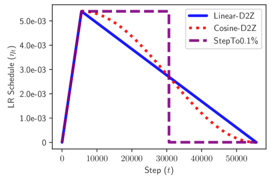
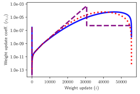
Figure 2: LR schedules and their update-combination duals: Each LR schedule, $\eta_{t}$ (left) and weight decay, $\lambda$, implies a weighted combination of weight updates, with combination coefficients $c_{t,i}$ (right, log-scale) giving the contribution of $i$th update to parameters $\theta_{t}$ at step $t$ (111M scale, coefficients at final step). The more sudden the drop in LR, the less emphasis on valuable later updates, perhaps explaining why Step underperforms Cosine and Cosine underperforms Linear decay.

To explain the success of Linear-D2Z, we build on recent work on the related topic of weight decay (Andriushchenko et al., 2023; Wang & Aitchison, 2024). First, decaying to zero helps because compute-efficient training includes a long phase in which gradient noise is the key factor slowing the loss reduction; with higher noise resulting from higher TPP or smaller batches, a vanishing LR works best. Second, we show that approaching zero linearly is beneficial via a novel interpretation of AdamW (Loshchilov & Hutter, 2017), the primary optimizer in LLM pre-training. With AdamW, weights generated at each step are implicitly a weighted combination of weight updates. The combination coefficients depend on the learning rate schedule and weight decay settings (Section 3.1). Analyzing this dual of the LR schedule, we observe linear decay to produce a favorable combination of prior weight updates (Figure 2). When LR drops abruptly, e.g., via step-decay or, to a lesser extent, cosine decay, later updates receive less emphasis, leading to worse model quality. The EMA dual perspective also reveals the implicit schedule-awareness of recent “schedule-free” approaches such as Warmup-Stable-Decay (WSD) (Hu et al., 2024; Bi et al., 2024; Hägele et al., 2024).

Our empirical study encompasses hundreds of models trained over a grid of schedules and peak LRs, with scales ranging from 111M to 1.7B parameters, and datasets up to 137B tokens. We also compare LR schedules over the cross product of weight decay versus peak LR, and peak LR versus batch size. We confirm a slight, consistent advantage of linear D2Z over cosine D2Z at 20 TPP. We also demonstrate that linear D2Z improves over continuous schedules such as WSD. Further, when dataset or batch size changes, optimal peak LRs are much more stable when using D2Z compared to using lesser decay. This latter finding exposes LR decay ratio as an important confounder in prior work studying optimal hyperparameter transfer with $\mu$P (Yang & Hu, 2020; Yang et al., 2021).

2 Background and Related Work

2.1 Learning rate schedules

LR schedules have a long history in stochastic optimization, and are motivated by convergence bounds for stochastic gradient methods (Moulines & Bach, 2011; Bottou et al., 2018). For example, following Andriushchenko et al. (2023), consider SGD for a convex loss parameterized by $\theta$: with a constant LR $\eta$, the gap between the optimum and current loss at step $t$ can be bounded by:

$$\mathbb{E}[\mathcal{L}(\theta_{t})-\mathcal{L}(\theta_{*})]\leq{\color[rgb]{0.12,0.98,0.64}(1-\eta\mu)^{t}||\theta_{0}-\theta_{*}||^{2}}+{\color[rgb]{1,.5,0}\eta\sigma^{2}}$$ (1)

where $\theta_{0}$ are initial parameters, $\theta_{*}$ is the loss minimizer, $\sigma^{2}$ is a bound on the variance of gradient noise, and $\mu$ is a measure of the objective’s curvature (see also Bottou et al. (2018, Theorem 4.6)). A larger LR can decrease dependence on initial conditions (the bias term), but also increase the effect of gradient noise (the variance term). As training progresses, bias decreases exponentially in $t$, and the relative importance of variance increases. Bottou et al. (2018) note this motivates a strategy where LR is high initially (to mitigate bias) and lowered later (to minimize variance).

In practice, when and how to reduce the LR is rarely informed by ML theory. Many LLMs simply follow the 10x cosine schedule, which is noted to work slightly better than cosine D2Z in the influential work of Hoffmann et al. (2022). It is also well established that using a portion of a longer (or extending a shorter) schedule is suboptimal compared to using a schedule that reaches its minimum only at the final training step (Li et al., 2019; Hoffmann et al., 2022; Hu et al., 2024; Hägele et al., 2024). Linear decay after warmup (Howard & Ruder, 2018) has been used in LLMs, typically also to 10% of the peak (Henighan et al., 2020; Dey et al., 2023; Sengupta et al., 2023). Dropping LR at specific milestones (step decay) is popular in vision models (He et al., 2016; Zagoruyko & Komodakis, 2016; Li et al., 2020), but has also been used in LLMs (Bi et al., 2024).

Kaplan et al. (2020) compared various decay functions and concluded the specific schedule was unimportant given a high enough average LR, although decaying to zero “gives a fixed improvement close to the end of training.” Few papers explicitly compare different LR schedules for large-scale training, and when comparisons are made (Shallue et al., 2019; Kaplan et al., 2020; Schmidt et al., 2021; Hoffmann et al., 2022; Yang et al., 2021), they are not the primary focus. So, while some insights are gained, “comprehensive study” is usually regarded as “out of scope” (Aleph Alpha, 2024). One exception is Defazio et al. (2023), who found linear equals or outperforms other common schedules, including cosine, across a range of problems, including LLM training. In addition, Defazio et al. develop convergence bounds that theoretically motivate linear as the optimal schedule. Unlike our work, they do not evaluate LLMs with different peak LRs or decay ratios.

Seeking to measure model quality at different training durations without having to re-train separate models from scratch (Zhai et al., 2022; Hägele et al., 2024), researchers have adopted various continuous schedules, such as constant, cyclic (Smith, 2017), etc. Following optimization theory (Moulines & Bach, 2011; Defazio et al., 2024) weight averaging provides an alternative to decay (Sandler et al., 2023; Sanyal et al., 2023; Busbridge et al., 2024), although it is typically not as effective (Hägele et al., 2024), and moreover may have hyperparameters that implicitly depend on training duration (Defazio et al., 2024). Warmup-Stable-Decay (WSD) approaches have also been used in LLM training (Hu et al., 2024; Shen et al., 2024a; Ibrahim et al., 2024; Hägele et al., 2024). These methods train at a constant LR, but decay from a checkpoint in a separate process when an intermediate model is needed. We show that the optimal constant LR of these methods implicitly depends on training duration, rendering them not truly schedule-free.

2.2 Maximal update parameterization ($\mu$P)

It is common to scale initial weights of neural networks such that activations have unit variance (Glorot & Bengio, 2010; He et al., 2015). Yet weights can become unstable after a few steps of updates, if layer-wise LRs are imbalanced (Yang et al., 2021). In contrast, $\mu$P (Yang & Hu, 2020; Dey et al., 2024a) prescribes a re-parameterization of initial weight variances and LRs – essentially, rules for scaling these values as model width (i.e., $d_{model}$) scales – so that activations and updates remain stable. $\mu$P also stabilizes embeddings, layer norms, and self-attention in Transformers. $\mu$P is seeing growing application in LLMs (Dey et al., 2023; Shen et al., 2024b; Hu et al., 2024), where it acts to stabilize training and to enable transfer of optimal hyperparameters (HPs) across model scales.

With $\mu$P, base HPs can be tuned on a small proxy, or base, model, and transferred to larger models. Given the width of the proxy model, $d_{p}$, and width of the target, $d_{t}$, $\mu$P prescribes scaling factors to apply to HPs. The base LR $\tilde{\eta}$ is scaled down to $\eta=\rho\tilde{\eta}$, where $\rho=\nicefrac{{d_{p}}}{{d_{t}}}$. In terms of LR schedules, the base LR $\tilde{\eta}_{t}$ is scaled at every step to provide $\eta_{t}$. $\mu$P is convenient in our study as we can sweep the same base peak LRs, $\tilde{\eta}$, at each model size, and observe trends that are scale-invariant.

2.3 AdamW weights as an exponentially-weighted moving average (EMA)

An AdamW update at a single training step, $t$, can be expressed as:

$$\theta_{t}=(1-\eta\lambda)\theta_{t-1}-\eta\frac{\hat{m}_{t}}{\sqrt{\hat{v}_{t}}+\epsilon}$$ (2)

where $\eta$ is the learning rate, $\hat{m}_{t}$ and $\hat{v}_{t}$ are (bias-corrected) running averages of the gradient and the squared gradient, respectively, and $\epsilon$ is a small constant added to prevent division by zero. The weight decay value, $\lambda$, is typically set to 0.1 in LLM training (Brown et al., 2020; Hoffmann et al., 2022; Almazrouei et al., 2023; Aleph Alpha, 2024).

While the running averages of $m$ and $v$ in Adam (Kingma & Ba, 2014) and AdamW are exponentially-weighted moving averages (EMAs), Wang & Aitchison (2024) recently showed that the weights generated by AdamW can also be understood as an EMA — of the weight updates. That is, a standard EMA, $y_{t}$, for a time-varying quantity, $x_{t}$, can be written as:

$$y_{t}=(1-\alpha)y_{t-1}+\alpha x_{t}$$ (3)

where $\alpha$ is the smoothing parameter. AdamW in Equation 2 can be seen as an EMA by letting:

$$y_{t}=\theta_{t}\mbox{, }\alpha=\eta\lambda\mbox{, and }x_{t}=-\frac{1}{\lambda}\frac{\hat{m}_{t}}{\sqrt{\hat{v}_{t}}+\epsilon}$$ (4)

Wang & Aitchison note the quantity $\tau$=$\nicefrac{{1}}{{\alpha}}$, i.e., $\nicefrac{{1}}{{(\eta\lambda)}}$, provides a rough timescale over which updates are averaged. Weight decay can therefore be used to control the effective window over which updates are combined (smaller values of $\lambda$ increase $\tau$, increasing the role of earlier updates in $\theta_{t}$). This perspective also motivates dynamic LR schedules. Initial $\tau$ should be small (high $\eta_{t}$), to forget early updates, “while the final timescale is around the total number of epochs [low $\eta_{t}$], to ensure averaging over all datapoints.” In fact, we will show that contribution of weight updates, $x_{0},x_{1},\ldots x_{t}$, to $\theta_{t}$ at a particular step, $t$, cannot be determined by the instantaneous value of $\eta_{t}\lambda$. Rather, the contribution of any $x_{i}$ to $\theta_{t}$ requires looking at the full LR schedule holistically (Section 3.1).

Wang & Aitchison also motivate scaling rules for optimal $\lambda$ as model and dataset size vary. If dataset size increases by a factor of $K$ (i.e., $K\times$ as many steps), the EMA perspective recommends scaling $\lambda$ by $\nicefrac{{1}}{{K}}$ in order to expand $\tau$ proportional to $K$. Moreover, with $\mu$P, if model size increases and LR is scaled by $\rho$ (Section 2.2), the EMA perspective motivates scaling $\lambda$ by $\nicefrac{{1}}{{\rho}}$ to keep $\tau$ constant.

3 Methods, Conceptual Foundations, and Hypotheses

We now present an extended EMA perspective on AdamW that accounts for time-varying LRs. We then introduce our conceptual model of LLM training, and connect it to the EMA perspective. Finally, we outline the specific testable hypotheses that follow from our conceptual model.

3.1 AdamW as convex combination of weight updates, driven by LR schedule

Consider a generic moving average, but now with time-varying smoothing, $\alpha_{t}$, i.e., $y_{t}=(1-\alpha_{t})y_{t-1}+\alpha_{t}x_{t}$. If we let $\alpha_{1}=1$ (so that $y_{1}=x_{1}$), we can express $y_{t}$ in terms of all inputs $x_{t}$:

$$y_{1} = \alpha_{1}x_{1},$$

$$y_{2} = (1-\alpha_{2})\alpha_{1}x_{1}+\alpha_{2}x_{2},\cdots$$

$$y_{t} = \sum_{i=1}^{t}\left(\prod_{j=i+1}^{t}(1-\alpha_{j})\right)\alpha_{i}x_{i}$$ (5)

$$= \sum_{i=1}^{t}c_{t,i}x_{i}$$

Where $c_{t,i}=\left(\prod_{j=i+1}^{t}(1-\alpha_{j})\right)\alpha_{i}$. It can be shown $\forall t,\sum_{i}c_{t,i}=1$, and hence, as in a standard EMA, each $y_{t}$ is a convex combination of inputs $x_{1}\ldots x_{t}$ (all coefficients are non-negative and sum to 1). However, with time-varying $\alpha_{t}$, we are not restricted to exponentially-decreasing $c_{t,i}$ as $i$ decreases. Indeed, for any convex combination of inputs, there is a corresponding smoothing schedule that generates the combination via the EMA. In terms of LR schedules for AdamW training, $y_{t}=\theta_{t}$, while $\alpha_{t}=\eta_{t}\lambda$ becomes the smoothing parameter at step $t$ (cf. Equations 3 and 4).

3.2 Conceptual model: bias and variance in LLM training

(a) Constant, fewer steps (low TPP)

(b) Constant, many steps (high TPP)

(c) D2Z, fewer steps (low TPP)

(d) D2Z, many steps (high TPP)

Figure 3: Bias & variance in LLM pre-training: as training duration increases (higher TPP), the importance of variance reduction — and having a lower LR — increases. With no decay (Constant, 3(a), 3(b)), the optimal peak LR must drop significantly lower, neglecting bias reduction. With D2Z (3(c), 3(d)), periods of bias and variance reduction can both be enjoyed without large shifts in peak LR.

Following Andriushchenko et al. (2023), our main conceptual premise is that in LLM training, there is an initial training phase focused on movement from initial conditions (bias reduction), followed by a later phase bottlenecked by gradient variance. Furthermore, analogous to prior work optimizing the convex loss gap via SGD (Equation 1), we argue the primary beneficial mechanism of LR decay in LLM training is to reduce gradient noise during later stages of training, while simultaneously minimizing the impact on bias reduction. The larger the dataset, the longer the proportion of training bottlenecked by gradient noise, and the greater the benefit from D2Z (Figure 3).

Variance reduction

Per-step gradient variance is known to increase over the course of training (McCandlish et al., 2018). Very recently, Zhang et al. (2024) showed that for an LLM of a fixed size, training with larger datasets corresponds to larger critical batch sizes, which directly relates to larger (aggregate) gradient variance via the gradient noise scale (McCandlish et al., 2018).

Figure 4: HP influence vs. TPP: Higher TPP means higher gradient noise; LR decay & weight decay settings thus increase in importance with TPP.

In the EMA perspective, parameters $\theta_{t}$ are a combination of prior weight updates (indexed by $i$). The more variance at step $t$, the more updates that should be combined in order to reduce it. Here variance is reduced by combining updates across steps, rather than increasing batch size at a specific step. Now, with a constant LR, update coefficient $c_{t,i}$ decreases exponentially in $(t-i)$: the further back the update from the current step, the less it contributes. But if LR $\eta_{i}$ decreases over steps, each later coefficient $c_{t,m}$ will be smaller due to a lower $\alpha_{m}=\eta_{m}\lambda$. Yet since coefficients sum to one, earlier coefficients will correspondingly increase: coefficients are basically flattened and updates contribute more evenly across steps. The more we decay, the more updates we average over, and the more variance is reduced.

Bias reduction

Higher decay is preferable to reducing peak LR because we must also minimize bias, i.e., the contribution of the initial random weights. In the EMA perspective, the contribution of these weights to $\theta_{t}$ is $c_{t,1}=\prod_{j=2}^{t}(1-\alpha_{j})$. For a decaying LR, and where $\alpha_{j}=\eta_{j}\lambda\ll 1$, coefficient $c_{t,1}$ can be approximated (with equality when LR is constant, Section B.1):

$$c_{t,1}\approx(1-\bar{\alpha})^{t-1}$$ (6)

where $\bar{\alpha}$ is the average $\alpha_{j}$ over the schedule. Exactly as in Equation 1, bias therefore decreases exponentially in the absolute number of steps, $t$, with a rate of decrease depending on the LR. Crucially, this means that as we train for more total steps (i.e., a higher tokens-per-parameter; TPP), there is a decrease in the fraction of steps required for $c_{t,1}$ to become negligible. At higher TPP, bias reduction becomes relatively less important than variance reduction (Figure 4).

3.3 Experimental Hypotheses

This hypothesis follows from the premise that gradient variance plays a larger role at higher TPP, and greater LR decay (as in D2Z) allows for more updates to be averaged, and thus greater variance reduction. A related hypothesis is that if we increase the batch size at each step, gradient variance will decrease, and so the benefits of D2Z over $\mbox{10}\times$ decay should diminish. Note our conceptual framework does not say precisely at which TPP or batch size that D2Z will first prevail; here we will rely on our empirical findings (Section 4) to fill in the theoretical gap.

Tuning peak LR is about trading off movement from initial conditions (requiring a high LR) and mitigating variance (requiring a low LR). As TPP increases, and bias reduction plays a smaller role, optimal peak LR should decrease. We hypothesize the decrease will be greater with a Constant schedule, as Constant does not use decay to balance the conflicting demands of bias and variance (Figure 3). Moreover, optimal peak LR for other continuous LR schedules, like WSD and Cyclic, should also decrease with longer training durations. In this way, such “schedule-free” approaches are not truly schedule-free. This dependence is also obvious when plotting update coefficients for these schedules (appendix Figure 29): the higher the LR, the more emphasis on recent updates.

While LR decay allows averaging over more weight updates, if the LR decreases too quickly, the final weight updates may not contribute to the EMA. From a loss surface perspective, as the LR approaches zero, we take vanishingly small steps. Since Cosine reaches smaller steps faster than Linear (Figure 2, left), Cosine will make less progress toward the optimum loss. From the EMA perspective, this is equivalent to Cosine having smaller $c_{t,i}$ coefficients as $i$ approaches $t$ (Figure 2, right). Note this problem is unique to Cosine D2Z and will not affect, e.g., Cosine $\mbox{10}\times$ decay.

Note that weight updates $x_{t}$ have a coefficient of $\nicefrac{{1}}{{\lambda}}$ in Equation 4. So, while $\eta_{t}$ and $\lambda$ contribute equally to $\alpha_{j}$, increasing $\lambda$ to reduce bias is counterproductive as weight updates will be scaled down proportionally, reducing movement from initial conditions. However, if LR is in a high enough range so that bias plays a minimal factor, both LR and WD should equally affect variance reduction.

4 Empirical Analysis of Decay-to-Zero

4.1 Experimental setup

Experiments use a GPT-like LLM (Radford et al., 2019), with ALiBi embeddings (Press et al., 2022) and SwiGLU (Shazeer, 2020). Main paper models are trained on SlimPajama (Soboleva et al., 2023) and evaluated over 1.1B held-out tokens (regardless of training TPP). Unless otherwise indicated, $\lambda$=$0.1$ is used. Training runs use the same random seed, so all decay functions (Linear, Cosine, etc.) and ratios (Constant, $\mbox{10}\times$, D2Z) have identical warmups, but note results are very consistent across seeds at this scale (appendix Figure 24). By default we use $\mu$P (standard parameterization results are in Sections C.2 and C.10). $\mu$P HPs are derived from a smaller proxy model tuned using a Linear-$\mbox{10}\times$ schedule. Since we hypothesized that different LR schedules may enjoy their optimal peak LR at different values, our experiments compare schedules when each is tuned to its optimal peak LR; we sweep $\tilde{\eta}$ by factors of 2$\times$ around the $\mu$P proxy-tuned $\tilde{\eta}=1.6\mbox{e-}02$. Appendix A provides further details on the model architecture (Table 2), dataset sizes (Table 3), and compute resources.

4.2 Results

Table 1: Comparison of schedules: validation loss for 610M $\mu$P models, 20 TPP. $\tilde{\eta}$=$1.6\mbox{e-}02$ is the $\mu$P proxy-tuned peak (base) LR, $\eta$ is the LR after $\mu$P adjustment ($\rho$=$0.125$, see Section 2.2). D2Z is superior to $\mbox{10}\times$ decay across most LRs. Linear-D2Z slightly outperforms Cosine-D2Z in all cases.

$\tilde{\eta}$	$\eta$	InvSqrt	Constant	Cosine	Linear	Cosine	Linear
				$\mbox{10}\times$	$\mbox{10}\times$	D2Z	D2Z
$6.5$e-$02$	$8.1$e-$03$	2.789	3.035	NaN	2.667	2.611	2.605
$3.2$e-$02$	$4.0$e-$03$	2.710	2.850	2.604	2.606	2.574	2.571
$1.6\mbox{e-}02$*	$2.0$e-$03$	2.671	2.768	2.590	2.591	2.578	2.573
$8.1$e-$03$	$1.0$e-$03$	2.665	2.722	2.598	2.600	2.595	2.590
$4.0$e-$03$	$5.1$e-$04$	2.691	2.711	2.634	2.635	2.637	2.633
$2.0$e-$03$	$2.5$e-$04$	2.762	2.739	2.707	2.710	2.717	2.714

For 610M-parameter $\mu$P models trained to compute-optimal 20 TPP, the optimal Linear-D2Z setting achieves 0.77% lower loss than the optimal Linear-$\mbox{10}\times$ setting (Table 1). At smaller, suboptimal peak LRs, $\mbox{10}\times$ can be better than D2Z. In appendix Figure 10, we demonstrate very similar results using the standard parameterization. Regarding the decay function, gains from Linear-D2Z over Cosine-D2Z are small, but perfectly consistent across peak LRs, exactly in line with recent work (Defazio et al., 2023; Lingle, 2024). Interestingly, Cosine-$\mbox{10}\times$ is consistently slightly better than Linear-$\mbox{10}\times$, showing that Linear itself is not always best, rather Linear plus D2Z is needed. Lacking a cooldown phase, inverse square root (InvSqrt) and Constant do not perform as well.

Appendix Figure 11 compares schedules as we sweep peak LR for 111M, 610M, and 1.7B models. For these and subsequent experiments, we use a Linear decay.

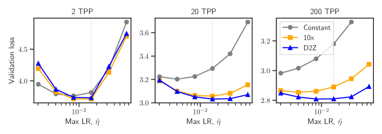
Figure 5: Comparing decay schedules across TPP (111M scale): As TPP increases, Linear-D2Z outperforms $\mbox{10}\times$, especially at the proxy-tuned peak LR (red lines).

For 111M models at only 2 TPP, D2Z performs worse than $\mbox{10}\times$ across all peak LRs (Figure 5, left). 610M results are similar (appendix Figure 12). However, as TPP increases, D2Z begins to outperform $\mbox{10}\times$, exceeding the best setting of $\mbox{10}\times$ by 1.6% at 200 TPP, and performing 2.8% better at the proxy-tuned $\tilde{\eta}$=$1.6\mbox{e-}02$ (marked in plots with a red vertical line). While we hypothesized D2Z would surpass $\mbox{10}\times$ at some TPP, our key finding is that, at both compute-efficient (20 TPP) and over-trained sizes, decaying to zero is optimal. Even at 2 TPP, some LR decay is beneficial ($\mbox{10}\times$ improves over Constant), but too much evidently hampers bias reduction. As TPP increases, optimal LRs for $\mbox{10}\times$ shift lower as variance reduction gains in importance, but now it is the lower peak LRs that hamper bias reduction, and $\mbox{10}\times$ begins to lag D2Z. By 20+ TPP, D2Z is consistently superior.

Figure 6 plots validation loss of $\mbox{10}\times$ and D2Z at different TPP settings for different model sizes (all models are trained using the proxy-tuned peak LR). For the 610M model, D2Z is also initially worse than $\mbox{10}\times$, but begins to surpass it around 4 TPP, and by 200 TPP is 2.6% better. As with training loss (Figure 1), an 80 TPP D2Z model can surpass a 200 TPP $\mbox{10}\times$ model in validation loss. Importantly, these trends also hold for downstream evaluation of the models (appendix Table 5).

Figure 6 also shows the advantage of using D2Z with 1.7B models trained to 80 TPP; D2Z achieves roughly 3.05% lower loss than $\mbox{10}\times$ at the proxy-tuned $\tilde{\eta}$. At this scale, such gains provide real-world impact: we over-train models of this size for use as proposal models in speculative decoding (Leviathan et al., 2023) and smaller models like Gemma-2B (Mesnard et al., 2024) and Phi-1.5 (Li et al., 2023) are used in many production settings.

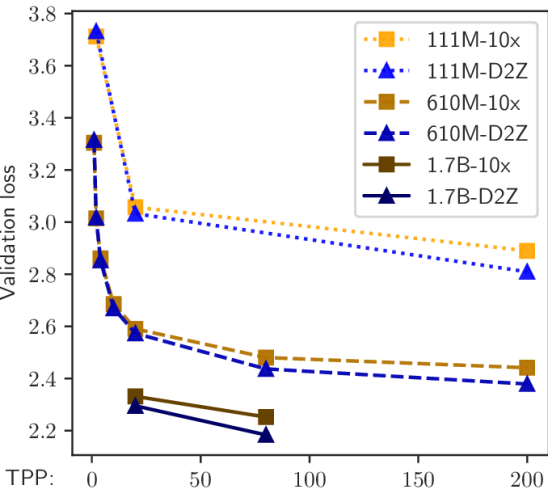
Figure 6: Loss gap between Linear-D2Z and $\mbox{10}\times$ grows with TPP: for 111M, 610M, and 1.7B-scale models.

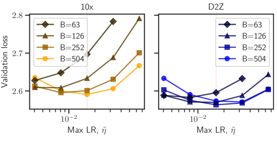
Figure 7: Comparison across batch sizes (iso-TPP) (610M): Comparing $\mbox{10}\times$ (left) to D2Z (right). All models trained to 20 TPP (smaller batches have more steps). As $B$ decreases, the optimal LR ($\tilde{\eta}$) drifts significantly lower for $\mbox{10}\times$ decay, less so for D2Z.

Figure 5 reveals different levels of hyperparameter sensitivity when increasing TPP: optimal LR shifts substantially lower for Constant, somewhat lower for $\mbox{10}\times$, and hardly at all for D2Z. The same trend holds at the 610M scale (appendix Figure 12). Moreover, with D2Z, loss is less sensitive to a suboptimal LR (bowls are flatter). D2Z loss is also more stable (and lower) as we vary both weight decay (appendix Figures 17 and 18) and batch size, $B$. For example, the optimal LR already shifts significantly for $\mbox{10}\times$ models at B=126, while D2Z optima only begin to shift at B=63 (Figure 7). The superiority of D2Z over $\mbox{10}\times$ across $B$ is more clearly observed in appendix Figure 13.

Crucially, if we keep the number of optimization steps constant (11752), but only vary $B$ (effectively increasing TPP proportional to $B$), we find the optimal learning rate does not decrease (i.e., with TPP) but rather increases (appendix Figure 14). Clearly, LR decay is primarily beneficial as a noise-reduction mechanism: with larger batches, we have less gradient noise, and can afford a larger LR.

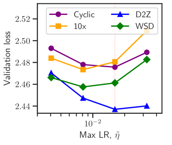
Figure 8: Comparison to continuous (610M, 80 TPP): D2Z surpasses Cyclic and WSD schedules.

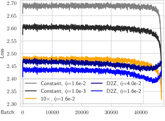
Figure 9: Loss on training set batches (in original order) after models have been trained (610M, 80 TPP)

In Figure 8, we compare D2Z to $\mbox{10}\times$, and to two approaches designed for continuous pre-training: Cyclic, which cycles LR up and down, and WSD (Section 2.1). For WSD, we simulate a model being retrieved after 80 TPP, and cool the LR to zero for the final 22.5% of steps (around the proportion recommended by Hägele et al. (2024), and equal to the cooldown duration in our 20 TPP models). Appendix Figure 29 provides full LR curves and update coefficients for all models in Figure 8.

At its optimal LR, WSD works better than $\mbox{10}\times$, confirming results in Hägele et al. (2024). However, note the optimal peak LR shifts lower for both $\mbox{10}\times$ and WSD at this TPP. Linear-D2Z remains best here, around 0.84% better than the optimal WSD. Given the diminishing returns of high-TPP training (Figure 6), WSD would require significantly more training FLOPs to reach the level of D2Z.

Figure 9 shows the loss of trained models (with frozen weights) on the exactly-same ordered batches used during pre-training. As predicted by the extended EMA perspective (Section 3), the higher the LR, the more models fit to late-stage training batches. It is striking that both Constant and $\mbox{10}\times$, but not D2Z, overfit to the very final portion. Extra adaptation of generative models to recent training sequences has long been observed (Graves, 2013), but to our knowledge this is the first evidence D2Z may help mitigate these effects. Since D2Z demonstrates the lowest loss on batches slightly before the final training phase, placing the highest-quality and most-recent data in the very final phase, while using D2Z (e.g., as in Dubey et al. (2024)), may be suboptimal. These findings also contradict Biderman et al. (2023), who found training order had little impact on memorization.

5 Discussion

The confounding role of LR schedule

We have shown that the more constant the LR schedule, the more sensitive the optimal peak $\eta$. These findings help explain LR sensitivity in prior work. For example, Shen et al. (2024b) were puzzled by their observation that “although the WSD scheduler could, in theory, continue in the stable phase forever …the optimal LRs are different for different amounts of training tokens.” As noted under Section 3.3, LR schedules with long constant periods only appear “schedule-free” in the primal; from the dual (EMA) perspective, the higher the LR, the more emphasis is placed on recent updates (see appendix Figure 28 for Constant, Figure 29 for WSD). Filatov et al. (2024) and Yang et al. (2021, Figure 19) also observed major decreases in optimal LR with higher TPP; these results were both obtained with a constant LR. In contrast, Bjorck et al. (2024) observed less significant decrease of optimal $\eta$ with TPP, but used $\mbox{10}\times$ decay.

LR schedule may also affect the optimal $\eta$ as batch size varies — particularly when using $\mu$P. Some prior $\mu$P studies (Yang et al., 2021; Noci et al., 2024; Shen et al., 2024b) observed linear scaling of optimal LR with batch size, i.e., the so-called linear scaling rule (Krizhevsky, 2014; Chen et al., 2016; Smith et al., 2018). Others (Lingle, 2024) have observed square-root scaling, resonating with other prior studies (Hoffer et al., 2017; You et al., 2019b; Malladi et al., 2022). This discrepancy can be explained by noting the linear scaling results were all found with a Constant or WSD LR decay, while square-root was observed with Linear D2Z, again underscoring the greater stability of D2Z.

The confounding role of training duration

While LR schedules have confounded studies varying TPP, TPP has analogously confounded studies evaluating LR schedules. Recall Kaplan et al. (2020) also saw a benefit from D2Z. In contrast to Chinchilla scaling (Hoffmann et al., 2022), in the Kaplan et al. perspective, small models should be trained to high TPP (while larger models should be trained less). It is therefore not surprising Kaplan et al. saw benefits testing D2Z with small models; as we have shown, D2Z is especially effective at high TPP. In contrast, in Figure 4 of Yang et al. (2021), Linear is worst of all schedules, and the gap between it and Constant and InvSqrt grows with model width. But here, since training data is small — and fixed, then TPP decreases as width increases. Thus training is in a phase where bias reduction is paramount and D2Z is not effective. Notably, in their LLM training experiments at higher TPP, Yang et al. do report linear D2Z to work best.

With this context, we speculate on why D2Z has not been adopted more widely in LLM pre-training:

• First, it is common to evaluate hyperparameters on smaller training runs; unfortunately, with limited training data (low TPP), D2Z misleadingly under-performs.

• Secondly, coupling between LR schedule and optimal peak LR is problematic: with $\mbox{10}\times$ decay, we may find a lower peak LR is optimal; if we then test D2Z with the same LR, it may be suboptimal for D2Z. Not seeing a benefit at this LR, we may conclude D2Z is inferior in general.

• Finally, poorly controlled training dynamics may prevent D2Z models from training with their (higher) optimal LR. Indeed, when we initially compared D2Z and $\mbox{10}\times$ using NanoGPT (Section C.10), $\mbox{10}\times$ performed better at the default LR. Raising the LR resulted in training divergence. Only after switching the numerical precision from bfloat16 to float32 could D2Z succeed — and the model reach optimal loss.

The special benefit of D2Z

Our results suggest a low $\alpha$ later in training can expand the timescale over which weight updates are combined, reducing noise in a similar way to increasing batch size. However, there is apparently a separate, independent benefit from a vanishing LR. Indeed, looking at appendix Figure 29 for the 80 TPP comparison to continuous schedules, we see $\mbox{10}\times$ coefficients are quite similar to the D2Z curve, apart from missing the final drop. Moreover, they are flatter than the WSD EMA coefficients for the same peak LR, suggesting better integration of prior updates. Yet WSD performs better than $\mbox{10}\times$ at all LR settings (Figure 8). In contrast, at 2 TPP (Figure 5, left), $\mbox{10}\times$ performs better than D2Z at every LR setting. Prior work has shown large LRs allow exploration of the loss surface at a height “above the valley floor” (Xing et al., 2018), while LR cooldown phases descend into a local minimum (Hu et al., 2024; Hägele et al., 2024). It appears that descending into these minima is beneficial only after sufficient exploration of the loss surface.

6 Limitations and Further Experiments

While our findings strongly support linear D2Z being optimal in our specific context, there are some limitations to keep in mind. First, LR schedules like D2Z require prior knowledge of the total number of training steps. But it is worth reiterating that even nominally schedule-free approaches such as Constant also require this knowledge in order to optimally set the LR value. In contrast, the extended EMA perspective of LR schedules enables derivation of a truly schedule-free schedule, which we introduce in Section D.1. Second, our focus in this paper was specifically LLM training at compute-optimal and overtrained dataset sizes. For ML problems with limited access to training data, D2Z is likely not the best strategy. Third, our work focuses on AdamW (the standard optimizer in LLM pre-training). While the extended EMA perspective of LR schedules will likely apply to other optimizers that use decoupled weight decay (as noted by Wang & Aitchison (2024)), it may not apply to approximate second order methods, such as Shampoo (Gupta et al., 2018). Finally, for LLMs with unstable training dynamics that cannot tolerate high LRs, D2Z may not be beneficial. We experienced this first-hand when we initially trained NanoGPT (Section C.10).

However, we also note the remarkable consistency of D2Z’s success. While results in the main paper used the SlimPajama dataset, consistent results were found with OpenWebText (Section C.10) and a multilingual dataset (with a larger vocabulary) (Section C.11). We also saw consistent findings with different parameterizations (Sections C.2 and C.10), architectures (Section C.11), weight sparsity settings (Section C.8), and training frameworks (Section C.10). Section C.11 describes scaling laws fit to models trained with D2Z and $\mbox{10}\times$, at model sizes up to 2.75B; results indicate a growing performance gap as scale increases. Finally, Section C.6 demonstrates that the benefits of weight decay are observed primarily when using LR D2Z, where raising weight decay can fine-tune the EMA update coefficients without affecting training stability.

7 Conclusion

Linear decay-to-zero is the optimal LR schedule for LLM training using AdamW. To be clear, less decay is beneficial for low tokens-per-parameter training, but there is no practical reason to perform such training with LLMs, since the same FLOPs could be used to train a smaller model, over more tokens, to a lower loss – using D2Z. The superiority of D2Z was validated across a range of experimental conditions. Results suggest its relative benefit will increase as models increase in scale. Moreover, when using D2Z and $\mu$P, the optimal peak LR is less sensitive to changes in weight decay, dataset size, and batch size, i.e., there is better hyperparameter transfer.

Our analysis was aided by our interpretation of AdamW’s output as a convex combination of prior weight updates. D2Z overfits less the final training sequences, and is especially beneficial when gradient noise dominates training. As we enter a phase of applied ML where inference efficiency is a primary concern, there is strong motivation to study high-TPP training, where gradient noise is the bottleneck. While our results indicate that D2Z is a key component of the solution here, further investigation is required, including into how and when to adjust hyperparameters such as weight decay, batch size, and learning rate, in the high-TPP context.

Appendix A Experimental Details

Table 2: Model architecture and batch sizes for main experiments

Model	vocab. size	$d_{model}$	$n_{layers}$	$d_{head}$	$d_{\text{ffn}}$	batch size
111M	50257	768	10	64	2048	192
610M	50257	2048	10	64	5461	504
1.7B	50257	2048	32	64	5461	504

Table 3: Training steps for main experiments

Model	TPP	Warmup	Steps	Tokens
111M	2	56	557	219M
111M	20	556	5568	2.19B
111M	200	5560	55680	21.9B
610M	2	118	1176	1.21B
610M	20	1175	11752	12.1B
610M	80	4700	47008	48.5B
610M	200	11750	117520	121B
1.7B	20	3322	33220	34.3B
1.7B	80	13288	132880	137B

Table 2 provides details on model architecture and hyperparameters for the main experiments (i.e., results presented in the main paper). Table 3 provides information on the training steps. All the models in our main experiments were trained on the SlimPajama dataset (Soboleva et al., 2023), a cleaned and deduplicated version of the RedPajama dataset. We use the GPT-2 (Radford et al., 2019) vocabulary of size 50257, and a context length of 2048 tokens. Unless otherwise noted, the weight decay value, $\lambda$, is by default set to 0.1, following standard practice in LLM pre-training (Brown et al., 2020; Hoffmann et al., 2022; Almazrouei et al., 2023; Aleph Alpha, 2024). Also following standard practice, we do not apply weight decay or bias to LayerNorm layers. Validation loss is always computed over 1.1B held-out tokens, regardless of training TPP. By default we parameterize with $\mu$P (further details below).

For a given TPP, all models have the exact same warmup phase: a linear warmup of the LR from 0 to the peak value. In all our runs, warmup was 10% of the total steps. LR warmup is standard practice in LLM pre-training.

All models in the main experiments were trained on a Cerebras CS-3 system. 610M-parameter, 20 TPP models take roughly 6 hours each to train on a single CS-3. If a training run did not complete due to numerical instabilities, the values are left off our plots or marked as NaN in Table 1.

Proxy model hyperparameter tuning

Table 4: Tuned hyperparameters for $\mu$P proxy model

$\sigma_{W,\text{base}}$	$8.67$e-$02$
$\tilde{\eta}$	$1.62\mbox{e-}02$
$\alpha_{\text{input}}$	$9.17$
$\alpha_{\text{output}}$	$1.095$

To find the optimal $\mu$P hyperparameters (HPs), we trained a 39M-parameter proxy model using a width $d_{\text{model}}$=$d_{p}$ of 256, with 24 layers and a head size of 64. We trained this proxy model on 800M tokens with a batch size of 256 and context length 2048, using $\mbox{10}\times$ decay. We randomly sampled 350 configurations of base learning rates, base initialization standard deviation, and embedding and output logits scaling factors, and used the top-performing values as our tuned HPs (Table 4).

Appendix B Derivations

B.1 Derivation of Equation 6

The initial coefficient is $c_{t,1}=\prod_{j=2}^{t}(1-\alpha_{j})$. Clearly, if $\alpha_{j}=\alpha$ is constant, we have $c_{t,1}=(1-\alpha)^{t-1}$. Otherwise, given $\alpha_{j}$ is small, we can use a first-order Taylor expansion, $e^{-\alpha_{j}}\approx 1-\alpha_{j}$, and therefore:

$$c_{t,1} \approx\prod_{j=2}^{t}e^{-\alpha_{j}}$$

$$=e^{\sum_{j=2}^{t}-\alpha_{j}}$$

$$=e^{-\sum_{j=2}^{t}\alpha_{j}}.$$

Assuming we only know the average value, $\bar{\alpha}=\frac{1}{t-1}\sum_{j=2}^{t}\alpha_{j}$, we have:

$$c_{t,1} \approx e^{-\bar{\alpha}(t-1)}$$

$$=(e^{-\bar{\alpha}})^{t-1}.$$

Given $\bar{\alpha}$ is also small, we reverse the earlier Taylor expansion, but now $e^{-\bar{\alpha}}\approx 1-\bar{\alpha}$, and:

$$c_{t,1} \approx(1-\bar{\alpha})^{t-1}.$$

That is, with a small time-varying smoothing parameter, the initial coefficient in an EMA, $c_{t,1}$, also decreases exponentially with the number of steps.

Appendix C Additional experimental results

In this section, we include some additional results to support the findings in the main paper. All validation losses reported in this section are from models trained with Linear decay.

C.1 Downstream evaluations

Table 5: Downstream evaluations: for 610M-parameter models corresponding to Figure 1. A model trained for 80 tokens-per-parameter with linear D2Z has equivalent downstream loss to the same model trained for 200 TPP with $\mbox{10}\times$ decay.

	MMLU (Avg.)	Commonsense Reasoning								Reading Comp.	Truthfulness & Bias		Down- stream (Avg.)
		Wino- grande	Hella- swag	Open- Book QA	Lamb- ada OpenAI	Lamb- ada Stand.	SIQA	PIQA	Arc-e	RACE	Truth- ful QA	CrowS- Pairs
$\mbox{10}\times$@80TPP	23.6%	52.2%	43.9%	31.4%	46.7%	36.7%	32.8%	68.7%	47.6%	32.3%	39.8%	60.7%	43.05%
D2Z@80TPP	23.5%	53.4%	44.6%	31.6%	46.9%	37.3%	33.2%	68.8%	48.8%	33.4%	40.2%	60.8%	43.54%
$\mbox{10}\times$@200TPP	23.3%	53.4%	46.6%	31.2%	46.2%	38.8%	32.2%	68.8%	47.9%	34.4%	38.4%	60.4%	43.46%
D2Z@200TPP	24.7%	54.5%	48.2%	32.4%	50.0%	42.6%	32.9%	70.1%	50.4%	32.6%	38.9%	62.5%	45.00%

Table 5 presents a variety of downstream evaluations of the four models presented in Figure 1. Differences between the models here are largely consistent with the differences in training and validation loss, showing that D2Z is meaningful not just for the autoregressive training objective, but for real-world applications.

C.2 Standard parameterization

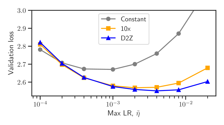
Figure 10: Standard parameterization results: Validation loss for different LR and decay combinations, across peak LRs, for 610M-parameter models trained with the standard parameterization.

Figure 10 presents results for a 610M-parameter model trained with the standard parameterization. Here $\tilde{\eta}$ is therefore not a $\mu$P-corrected base LR, but rather a LR that we swept directly for this model scale. Results are obviously quite similar to results using $\mu$P, suggesting the benefits of D2Z are not $\mu$P-specific. Further results using the standard parameterization, but for NanoGPT models, are in Section C.10 below.

C.3 Model sizes

Figure 11: Model size comparison: Validation losses at 20 TPP. Across all model sizes, Linear-D2Z outperforms Linear-$\mbox{10}\times$. Note: Missing high-LR values in all plots correspond to failed training runs due to NaN instabilities.

Figure 11 presents results across 111M, 610M, and 1.7B model sizes, all trained to 20 TPP. Note the absence of results for the highest LR setting at the 1.7B-scale; at the very highest LR, numerical instabilities led to failed training runs. Otherwise, results are fairly similar across model sizes. At the proxy-tuned peak LR, the gap between D2Z and $\mbox{10}\times$ is 0.81%, 0.67%, and 1.56%, at the 111M, 610M, and 1.7B scales, respectively. We further investigate the issue of whether the gap between D2Z and $\mbox{10}\times$ varies with model size as part of our scaling law experiments below (Section C.11).

C.4 TPP

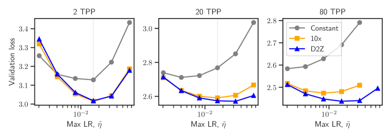
Figure 12: Comparing decay schedules across TPP (610M scale): As TPP increases, Linear-D2Z begins to outperform Linear-$\mbox{10}\times$, especially at the proxy-tuned peak LR (red lines). The optimal LR also shifts significantly lower for Constant, somewhat lower for $\mbox{10}\times$, and hardly at all for D2Z. Compare to Figure 5 for 111M models.

As we vary TPP, we consistently see increasing gains with D2Z. Here we plot the results for the 610M-scale models in Figure 12, as a counterpart to main Figure 5.

C.5 Batch sizes

Batch size setup

Default batch sizes of 192 and 504 (Table 2) were selected for 111M and 610M scales. These specific values were based on an internal scaling law for optimal batch size as a function of compute FLOPs (similar to those in Bi et al. (2024) and Porian et al. (2024)). Batch size of 504 was then re-used for 1.7B training (later testing confirmed this to be a good setting at 1.7B for 20 TPP training). In our experiments varying batch size, we swept $B$ by factors of 2 around these initial settings.

C.5.1 Iso-TPP batch size experiments

Figure 13: Comparison across batch sizes (iso-TPP) (610M): Different batch sizes, $B$, but all trained to 20 TPP. As batch size decreases, the relative gain of D2Z over $\mbox{10}\times$ increases. Same data as in Figure 7.

In main paper Figure 7, we presented results where all models train for the same number of total tokens (20 TPP), while only the batch size, $B$, varies. Figure 13 presents the same data, but with each $B$ separated into a separate subplot; this lets us better observe how the differences between D2Z and $\mbox{10}\times$ evolve as $B$ changes. We see clearly that for smaller $B$, as gradient noise increases, the differences between D2Z and $\mbox{10}\times$ also increase. This again demonstrates that LR decay is beneficial as a noise reduction mechanism.

We now discuss the related observation that the optimal LR decreases as $B$ decreases. Note the EMA perspective of Wang & Aitchison (2024) would predict linear scaling of $\tilde{\eta}$ with $B$. This is because the total number of iterations scales with $1/B$. Therefore, in order to keep the timescale constant (as a fraction of the total iterations), we would need to scale $\tilde{\eta}$ (or $\lambda$) proportional to any change in $B$. Although we do see roughly linear scaling in the case of $\mbox{10}\times$ models, the optimal $\tilde{\eta}$ is more stable with D2Z. In our conceptual model, the purpose of the timescale is to optimize variance reduction. But note that lowering $\tilde{\eta}$ also has an effect on bias reduction. For $\mbox{10}\times$, as $B$ changes, it seems paying the cost of lower bias reduction is worth the benefits in variance reduction. Since using D2Z already enables better variance reduction, it seems, for D2Z, lowering $\tilde{\eta}$ has less value in the trade-off, so optimal $\tilde{\eta}$ lowers to a lesser extent.

C.5.2 Iso-step batch size experiments

Figure 14: Comparison across batch sizes (iso-step) (610M): Different batch sizes, $B$, but all trained for 11752 steps (not iso-FLOP, smaller batches see fewer TPP). In contrast, Figure 7 and appendix Figure 13 instead keep TPP constant. D2Z remains superior in the iso-Step context. More interestingly, here the optimal LR actually increases as batches — and, correspondingly, the datasets — increase in size.

In the above batch size tests, we kept the dataset size constant (iso-TPP). Now consider the following two mechanisms for increasing the dataset size (TPP) of a training run:

1. Fix the batch size, but increase the number of steps.

2. Fix the number of steps, but increase the batch size.

Approach (1) was taken in our experiments increasing TPP. In that case, we found optimal LR to decrease, as a mechanism for coping with greater gradient noise, which grows with TPP. We now discuss Approach (2): fixing the number of steps, but increasing the batch size (iso-step).

In Figure 14, we keep the number of steps constant to 11752, so each model will see the same total number of batches, and we increase $B$ by factors of two. Since number of steps does not change, Wang & Aitchison (2024) do not prescribe any adjustments to the timescale, and hence no adjustment is needed to LR (or weight decay). But we clearly see that optimal LR increases as $B$ increases (like a rolling wheel, LR bowls rotate clockwise as we move to the right). This is evidently because increasing $B$ decreases gradient noise; with less noise, we can afford a larger LR throughout training. More precisely, increasing $\tilde{\eta}$ decreases the number of AdamW weight updates that are combined. Therefore, an increase in $\tilde{\eta}$ can be viewed as a way to reduce the effective number of batches that are combined, basically compensating for the fact per-step $B$ is larger.

As $B$ increases, gradient noise decreases, and we would expect benefits of LR decay to also diminish; differences between $\mbox{10}\times$ and D2Z do seem to decrease. This aligns with prior work, e.g., You et al. (2019a) compared SGD to full-batch GD (with WideResNets for image classification), and showed that when gradient noise is eliminated by using full GD, LR decay is no longer beneficial.

C.6 Weight Decay

C.6.1 Weight decay: results

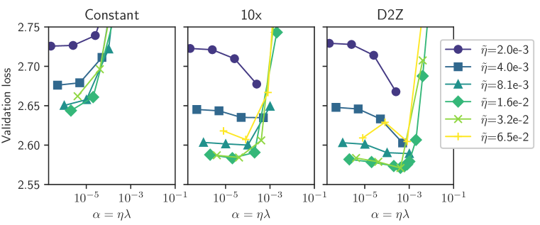
Figure 15: Weight decay results, grouped by $\tilde{\eta}$ as $\alpha$=$\eta\lambda$ varies (610M, 20 TPP): Validation losses for different settings of decay schedule (separated by subplot), maximum learning rate ($\tilde{\eta}$, marked by color), and weight decay ($\lambda$, corresponding to points on the LR curves). Loss is plotted relative to $\alpha$=$\eta\lambda$. The optimal loss corresponds to high (but not too high) $\tilde{\eta}$. As the smoothing $\alpha$ increases, Constant models suffer, $\mbox{10}\times$ models see marginal gains, while D2Z models benefit significantly.

Figure 15 analyzes the interaction between weight decay (WD) and LR for 610M models. Here we plot with the x-axis set to the (peak) smoothing parameter, $\alpha$=$\eta\lambda$ (on a log scale), and y-axis set to validation loss. Note that for a given decay ratio and fixed $\alpha$, EMA update coefficients (Section 3) are identical (i.e., specific values of $\eta$ and $\lambda$ do not affect coefficients, only their product). Thus it supports the extended EMA perspective to note that regardless of peak LR, $\tilde{\eta}$, models tend to reach lowest loss at around the same $\alpha$ (Figure 15); that is, the same EMA timescale, $\nicefrac{{1}}{{\eta\lambda}}$, is optimal across different LRs. However, to reach optimal loss, models require $\tilde{\eta}$ to be high enough, but not too high — at $\tilde{\eta}$=$6.5$e-$02$ and above, we consistently encounter instabilities in training.

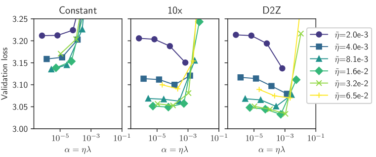
Figure 16: Weight decay results, grouped by $\tilde{\eta}$ as $\alpha$=$\eta\lambda$ varies (111M, 20 TPP): Validation losses for different settings of decay schedule (separated by subplot), maximum learning rate ($\tilde{\eta}$, marked by color), and weight decay ($\lambda$, corresponding to points on the LR curves). Loss is plotted relative to $\alpha$=$\eta\lambda$. The optimal loss is obtained when $\tilde{\eta}$ is high, but not too high, typically around $1.6\mbox{e-}02$ to $3.2$e-$02$. As in Figure 15, only D2Z models further improve as $\lambda$ increases.

When increasing $\lambda$ with a given peak LR (moving left-to-right along curves), note behavior differs depending on LR schedule: Constant models perform worse, Linear-$\mbox{10}\times$ sees marginal gains, and Linear-D2Z benefits significantly. Results are similar for 111M models (Figure 16).

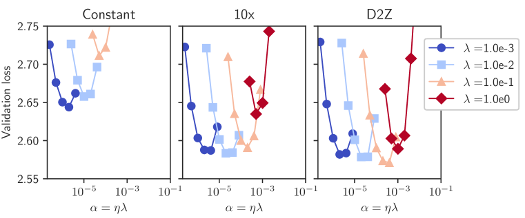
Figure 17: Weight decay results, grouped by $\lambda$ as $\alpha$=$\eta\lambda$ varies (610M, 20 TPP): Subset of the data in Figure 15, but now curves trace points with same weight decay $\lambda$ (in color) and LR $\eta$ varies across each curve. Only D2Z models significantly improve as we increase weight decay. D2Z models are also less sensitive to choice of $\lambda$.

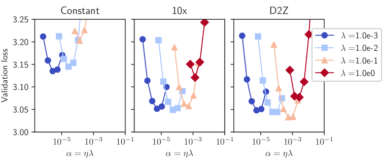
Figure 18: Weight decay results, grouped by $\lambda$ as $\alpha$=$\eta\lambda$ varies (111M, 20 TPP): Same data as in Figure 16, but now curves trace points with same weight decay $\lambda$ (in color) and LR $\eta$ varies across each curve. Only D2Z models significantly improve as we increase weight decay. D2Z models are also less sensitive to choice of $\lambda$. See Figure 17 for 610M-model results.

Figures 17 and 18 depict the same data, but with points now grouped by $\lambda$. For higher or lower $\lambda$, we cannot reach the optimal timescale without taking $\tilde{\eta}$ out of its comfort zone. Therefore, with our 20 TPP models, $\lambda$=0.1 emerges as good default setting because, in synergy with a comfortable LR, $\lambda$=0.1 corresponds to an appropriate EMA timescale.

Similar to the findings in Andriushchenko et al. (2023), we also confirm weight decay does not act like a traditional regularizer here: beneficial settings of weight decay always improve both validation and training loss.

C.6.2 Weight decay: further discussion

Learning rates reduce bias, weight decay best controls variance

Recall that Section 3.3 made the observation that while LR $\eta$ and weight decay $\lambda$ can both equally change the update coefficients, only $\eta$ is effective in moving the model away from initial conditions (due to the $\nicefrac{{1}}{{\lambda}}$ factor applied to the updates). This is confirmed by Figures 15 and 16: only when $\eta$ is sufficiently high do models achieve optimal loss. Given such a high-enough $\eta$, the primary benefit of weight decay is evidently to adjust $\alpha$=$\eta\lambda$ (and hence the timescale $\nicefrac{{1}}{{\alpha}}$), to a setting that synergizes best with the decay schedule (for 610M models, around $4$e-$04$). Weight decay is specifically useful in this context because training instabilities prevent reaching this optimal $\alpha$ purely through increasing $\eta$. However, given $\eta$ and $\lambda$ both affect the timescale, $\alpha$=$\eta\lambda$ can be viewed as the effective or intrinsic LR (Li et al., 2020; Wang & Aitchison, 2024), but only later in training.

Since weight decay does not impact bias reduction, it follows that, when the timescale needs to be adjusted at high TPP due to the greater gradient noise, it should be more effective to lower WD than to lower LR, exactly as prescribed by Wang & Aitchison (2024). In ongoing concurrent work, we do observe lower loss from tuning WD compared to tuning LR. This stands in contrast to other recent work that recommends purely decreases in LR for high-TPP training (Shen et al., 2024b; Bjorck et al., 2024).

Why weight decay is only beneficial when using LR decay

Our observation that weight decay is only beneficial when using a LR (decay) schedule aligns with both Loshchilov & Hutter (2017) and Andriushchenko et al. (2023) who also observed no benefit from WD when using constant LRs. In contrast, Aleph Alpha (2024) recently reported $\lambda$=$0.1$ to improve over $\lambda$=$0.0$ in LLM training; notably, they train with D2Z. We believe the reason for these observations can also be explained by the bias/variance trade-off, and by the fact, noted above, that weight decay primarily plays a role later in training. Since its LR is fixed, Constant negotiates the bias/variance trade-off by using a LR that is suboptimally low early and suboptimally high later on (refer back to Figure 3 in the main paper for a visualization). Increasing $\lambda$ raises the already-too-high (late) $\alpha$ even higher, further decreasing the timescale $\nicefrac{{1}}{{\alpha}}$ and hurting the model. In contrast, when using a LR schedule, weight decay can play its beneficial variance reduction role, as discussed above.

It is also worth observing that if one is using D2Z with a LR that is suboptimally low (e.g., if increasing it any further caused numerical stability issues, as we observed with NanoGPT in Section C.10), then increasing weight decay can be very beneficial. For example, note the large improvements in loss as weight decay is increased for the $\tilde{\eta}$=$4.0$e-$3$ and $\tilde{\eta}$=$2.0$e-$3$ curves in Figure 15.

Stability of D2Z loss with high $\lambda$

While Constant and $\mbox{10}\times$ are much worse at higher $\lambda$ values, D2Z performs reasonably well even at $\lambda$=$1.0$ (particularly at the 610M scale). Since increasing $\lambda$ effectively decreases the timescale $\nicefrac{{1}}{{\alpha}}$ over which weight updates are integrated, it increases the variance over weight updates. Therefore, setting $\lambda$ too high hurts all models, but since D2Z has lower $\eta$ later in training, it somewhat counterbalances the increase in $\lambda$ in the product $\alpha$=$\eta\lambda$. Another view of this is that as fewer updates are combined, noise increases; D2Z is evidently best at mitigating the negative effects of such noise through its maximal LR decay.

C.7 Step decay

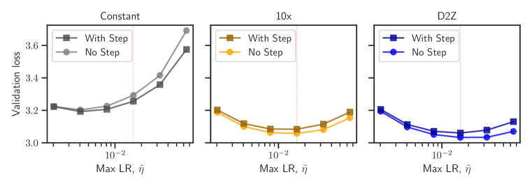
Figure 19: Impact of applying Step decay (111M, 20 TPP): Validation loss for different LR and decay combinations with and without Step decay. Step decay is applied after 90% of training, stepping to a value equal to 0.1% of the maximum LR. Dropping the LR in this manner helps Constant, although it is still below the level of $\mbox{10}\times$ and D2Z. Adding stepping to a $\mbox{10}\times$ or D2Z schedule is not beneficial.

In Figure 19, we present results investigating the impact of Step decay on model training. Here, for 111M-parameter models, Step decay can improve the loss versus keeping the LR constant (left panel), but the resulting losses are still much worse than those obtained with D2Z or $\mbox{10}\times$ decay. We also tried applying a Step decay to a LR that had been following a $\mbox{10}\times$ (middle panel) or D2Z trajectory (right panel); this approach always led to inferior results.

While it is likely possible to improve the quality of Step decay by tuning the positioning of the drop, we hypothesize that these efforts will not surpass D2Z, since dropping the LR will fundamentally always result in an over-emphasis of earlier updates, as shown in Figure 2 and Figure 27. Moreover, introducing additional tunable hyperparameters (i.e., when and how much to decay) is a further drawback of the Step schedule.

C.8 Weight sparsity

Weight sparsity setup

In this section, we investigate the role of Linear-D2Z in the context of models trained with unstructured weight sparsity, a promising direction for improving the efficiency of large neural networks (Hoefler et al., 2021). We parameterize with $\mu$P’s sparse extension, S$\mu$Par (Dey et al., 2024b). S$\mu$Par allows us to use the same $\mu$P hyperparameters as with dense models, except we must now apply corrections due to both model scaling (i.e., $\rho$, Section 2.2) and layer sparsity. For these experiments, we sparsified all non-embedding layers of our 610M-parameter dense models by randomly fixing certain weights to zero for the duration of training. We trained all models for 11752 total steps using a batch size of 504, i.e., the same amount of training data as we used for training the corresponding 610M-parameter dense models to 20 TPP (Tables 2 and 3).

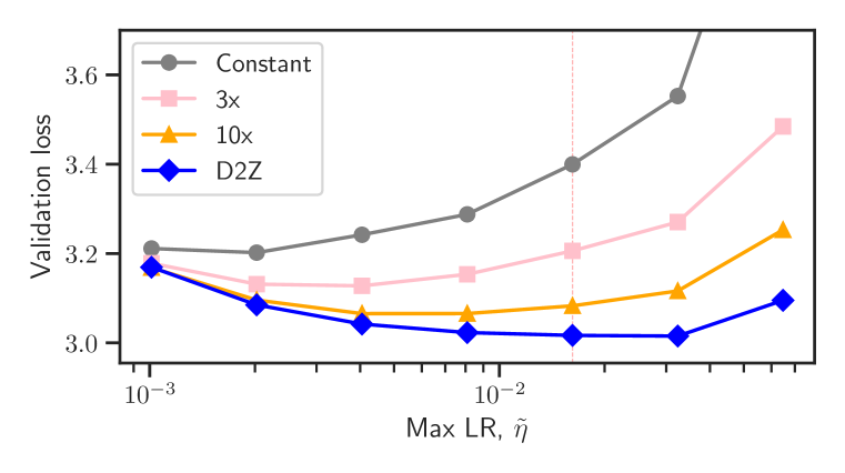
Figure 20: Comparison of decay schedules when using 93.75% weight sparsity (610M): Validation losses for different LR and decay combinations, for a model trained with S$\mu$Par, with 93.75% unstructured weight sparsity. As the decay rate increases, loss improves, while the optimal peak LR is much more stable when using D2Z.

At 93.75% sparsity ($\nicefrac{{1}}{{16}}$ density), the optimal D2Z model improves by 1.64% over the optimal $\mbox{10}\times$ model, with a clear trend of optimal LRs shifting lower and loss becoming worse as we go from $\mbox{10}\times$ to $3\times$ to Constant decay (Figure 20).

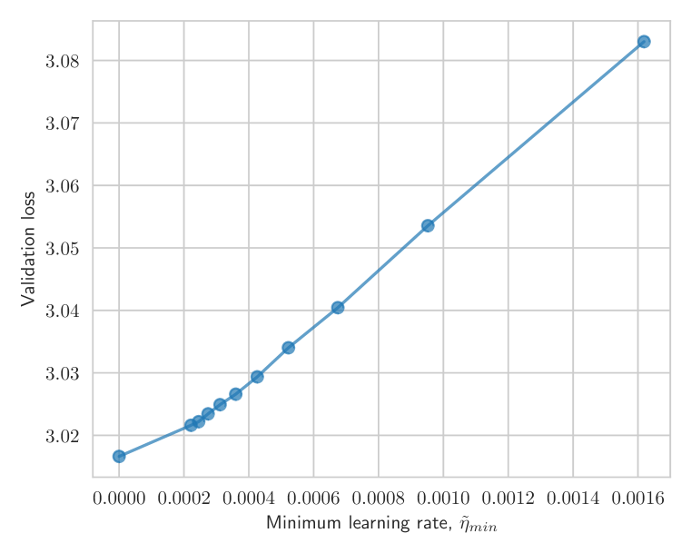
Figure 21: Decay ratio sweep, part 1 (610M): Validation loss for models trained with S$\mu$Par, with 93.75% unstructured weight sparsity, as we vary the LR decay ratio. The x-axis plots the minimum LR, i.e., the LR at the final training step. As the ratio increases from $\mbox{10}\times$ (right-most point), where the minimum LR is 10% of the proxy-tuned rate, to 0% (D2Z, left-most point), validation loss decreases roughly linearly.

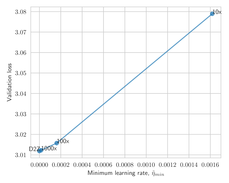
Figure 22: Decay ratio sweep, part 2 (610M): Validation loss for models trained with S$\mu$Par, with 93.75% unstructured weight sparsity, for a LR decay ratio of $\mbox{10}\times$, $\mbox{100}\times$, $\mbox{1000}\times$, and D2Z (using a different sparsity pattern than part 1). As in part 1, validation loss decreases roughly linearly with the minimum LR.

At the proxy-tuned peak LR of $1.6\mbox{e-}02$, D2Z is 2.15% better than $\mbox{10}\times$. We also trained 93.75% sparse models with a variety of other decay ratios between $\mbox{10}\times$ and D2Z, and present these results in Figures 21 and 22. Here we see a largely linear decrease in loss with a linear increase in the decay ratio (i.e., a linear decrease in the minimum LR). These are encouraging findings in the sense that D2Z can seemingly be used directly on a range of problems, without having to worry about tuning a problem-specific LR decay ratio (e.g., 50$\times$ or 100$\times$).

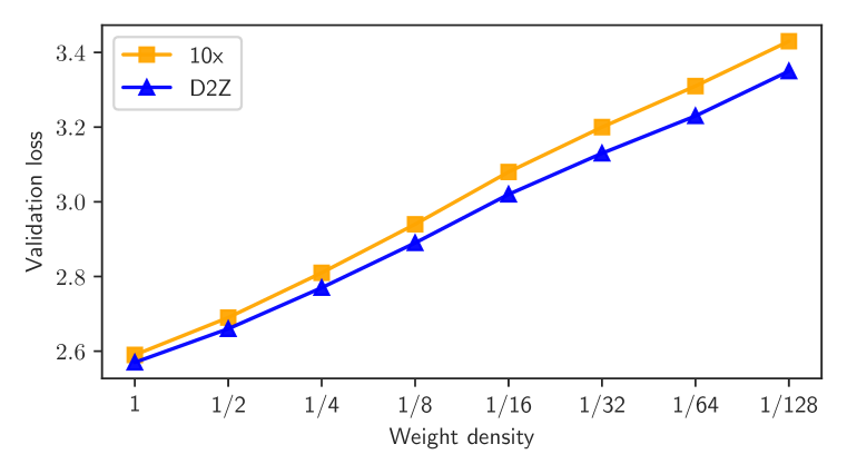
Figure 23: Comparison of decay schedules when using varying weight sparsity (610M): Validation losses for models trained with S$\mu$Par, as unstructured weight sparsity increases (density decreases). All models trained with the same number of training tokens (11752 steps, equivalent to 20 TPP for the fully-dense models). As sparsity increases, the number of trainable parameters decreases, and thus tokens-per-(non-zero)-parameter (and the benefit of D2Z) increases.

In Figure 23, we investigate the gap between D2Z and $\mbox{10}\times$ at the proxy-tuned peak LR across different sparsity levels. Note that increasing sparsity effectively leads to a corresponding decrease in the number of trainable parameters. Since we use a fixed number of training tokens in each case, as the number of parameters decreases, the number of tokens-per-parameter (TPP) increases. In this sense, we note the relative differences between D2Z and $\mbox{10}\times$ are consistent with our results in Figure 6 — as TPP (and gradient noise) increases, D2Z performs relatively better.

C.9 Error bars

Figure 24: Stability across random seeds (111M, 20 TPP): Validation loss variance for different maximum LRs at different decay ratios. Each point corresponds to the mean validation loss over 5 separate training runs with different random seeds; the error bars give the standard deviation. Beyond the instabilities at high learning rates, run-to-run variance is remarkably low at this scale.

Taken as a whole, our results are remarkably stable: empirical results for different model scales, training durations, batch sizes, weight decays, and weight sparsity settings largely behave as predicted by theory. Since all validation runs are performed on 1.1B tokens, any significant run-to-run variance must arise during training. To quantify this variance, we repeated 111M-model 20 TPP training four additional times, resulting in 5 total validation loss results for each original training run. Figure 24 confirms that run-to-run variance is remarkably low. The only significant variance arises in Constant results at the highest learning rate. Here, the training loss sometimes spikes at various points during training, and the final validation loss can be significantly higher for models that cannot recover sufficiently following the spike.

C.10 NanoGPT experiments

We also compared $\mbox{10}\times$ versus D2Z by training NanoGPT models using the NanoGPT codebase (Karpathy, 2024). NanoGPT uses the standard parameterization. We configured these models to be largely similar to our 111M-parameter models, also using a weight decay of 0.1, a context length of 2048, and the GPT-2 vocab size of 50257. Key differences here are that we do not include bias weights, and we trained on the OpenWebText dataset (Gokaslan & Cohen, 2019). Experiments are run on Nvidia A10 GPUs.

As mentioned in Section 5, we initially tested NanoGPT in bfloat16 precision. Here, at the default NanoGPT learning rate of 6e-4, $\mbox{10}\times$ performed slightly better than D2Z. As we pushed the LR 50% higher (to 9e-4), both $\mbox{10}\times$ and D2Z had higher loss, and by 1.2e-3, the loss from $\mbox{10}\times$ doubled.

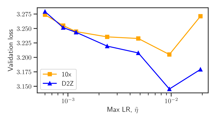
Figure 25: NanoGPT results (111M, 20 TPP): Validation loss for different LR and decay combinations, for a NanoGPT model. With float16 precision, we were not able to train above $6$e-$04$ without instabilities (first point in curves). Moreover, at $\tilde{\eta}=6$e-$04$, $\mbox{10}\times$ performed better than D2Z. After switching to float32, we were able to train at higher $\tilde{\eta}$ values, where D2Z demonstrates its familiar superiority over $\mbox{10}\times$.

We suspected that numerical issues may be causing the instabilities, and repeated our experiments in float32. At this precision, we were able to successfully increase the LR, by factors of two, up to 32 times the default. At these levels, we do see the familiar gains of D2Z over $\mbox{10}\times$ (Figure 25). We note there is nothing fundamentally limiting about float16 precision itself - indeed all our main experiments were done using this precision. Rather, float16 is simply problematic at a high learning rate in the NanoGPT codebase (see Gray et al. (2024, Appendix C.2) for a potential root cause of this instability).

These experiments demonstrate that a comparison between D2Z and $\mbox{10}\times$ may serve as a kind of diagnostic of whether a model is being trained at optimal peak LRs: if a 100M+ model trained to 20 TPP does not see roughly 1% gains from using D2Z, it is likely the LR is not high enough. In order to raise the LR further, efforts to stabilize the model, perhaps including $\mu$P or other techniques (Wortsman et al., 2023), may be warranted.

C.11 Scaling law experiments

Encouraged by the results of D2Z at smaller scales, we began testing D2Z in some of our frontier model efforts. Frontier models do not provide scope for hyperparameter tuning at scale. Thus it becomes important to derive scaling laws to forecast loss at larger scales, based on the loss with a sequence of smaller models.

For this set of experiments, we tested Llama-style (Touvron et al., 2023a) architectures, except using LayerNorm instead of RMSNorm, and multi-head attention instead of group-query attention. We use $\mu$P here as well, and a batch size scaling law to determine an optimal batch size for each model scale. These models also use ALiBi embeddings (Press et al., 2022) and SwiGLU (Shazeer, 2020). Here, the context length is 8192 tokens, and we use tied embeddings. We also re-tuned our $\mu$P proxy-model hyperparameters.

We used a bilingual data mix of English, Arabic and source code samples mixed in a 2:1:0.4 mix ratio. English data is from the Pile (Gao et al., 2020), Arabic uses a proprietary dataset (Sengupta et al., 2023), and the source code comes from the GitHub portion of the Pile.

Table 6: Model architecture and batch sizes for scaling law experiments.

Model	vocab. size	$d_{\text{model}}$	$n_{\text{layers}}$	$d_{\text{head}}$	$d_{\text{ffn}}$	batch size
272M	84992	1024	14	64	2912	128
653M	84992	1536	18	128	4096	160
1.39B	84992	2048	24	128	5472	208
2.75B	84992	2560	32	128	6832	256

To derive scaling laws to compare D2Z and $\mbox{10}\times$ models, we used the power law functional form $y=cx^{m}$, where $x$ is the pre-training FLOPs, $y$ is the loss on the Pile validation set, and $c$ and $m$ are parameters to be fit. To fit these parameters, we transformed our Loss-to-FLOPs equation, $y=cx^{m}$, to a logarithmic form, $log(y)=log(c)+mlog(x)$, and fit the slope and intercept parameters of this line using a least-squares linear regression. We trained models at four sizes to compute-optimal 20 TPP (Table 6), and computed total FLOPs spent as well as validation loss on the Pile. We then fit the power law free parameters to obtain our scaling laws.

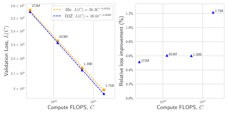
Figure 26: Scaling law comparison of decay schedules: Loss-to-FLOPS scaling law fits for models trained to 20 TPP (8192 context lengths, Llama architecture, Pile validation data). The power law fit for D2Z models has a steeper slope than the scaling law for $\mbox{10}\times$ models, implying a growing performance gap for larger model sizes.

Encouragingly, here we find the scaling law slope of D2Z is roughly 2.5% better than $\mbox{10}\times$ decay (Figure 26). This translates to an improvement of roughly 1% at 1.3B and 2.7B scales, broadly similar to our earlier results at 1.7B scale. Projecting our scaling law to a 70B model trained to a compute optimal 20 TPP, D2Z would achieve a roughly 2% loss improvement over $\mbox{10}\times$ decay.

Appendix D AdamW as convex combination of weight updates, driven by LR schedule: Further details

We have begun using plots of the weight update coefficients internally to proactively analyze LR schedules. These plots give us insight into the timescale over which training data is integrated into the model parameters, and can be obtained without actually performing any training. Moreover, we can also use the extended EMA perspective in order to design novel LR schedules that have desirable blends of weight updates. Optimizing these coefficients thus provides a dual to optimizing the LR decay function, which is why we refer to these coefficients as the dual coefficients of the LR schedule. In this section, we first describe the design of one such LR schedule, and then we follow with example plots for this and other schedules.

D.1 Truly schedule-free LR schedules

Recall that, for a moving average with time-varying smoothing, $y_{t}=(1-\alpha_{t})y_{t-1}+\alpha_{t}x_{t}$, we use $c_{t,i}=\left(\prod_{j=i+1}^{t}(1-\alpha_{j})\right)\alpha_{i}$ to denote the dual coefficients, i.e., the contribution of input $x_{i}$ to output $y_{t}$ at time $t$. Constant schedules, or schedules with a long constant phase such as WSD, are not truly “schedule-free” because their peak LR setting affects the $(1-\alpha_{j})$ terms in the dual. Different LRs will correspond to different effective timescales over updates, and thus different LRs will be optimal for different training durations.

In contrast, we now derive a schedule such that coefficients are always weighted equally, at every training step. First, it can be shown that:

$$\frac{c_{t,i+1}}{c_{t,i}}=\frac{\alpha_{i+1}}{(1-\alpha_{i+1})\alpha_{i}}.$$ (7)

For the coefficients to be uniform at any step $t$, we require this ratio to be 1. Unity of this ratio implies that smoothing evolves $\alpha_{i+1}$ = $\frac{\alpha_{i}}{(1+\alpha_{i})}$. Assuming a fixed weight decay (so $\alpha_{i}=\eta_{i}\lambda$), coefficients will be equal if the LR evolves:

$$\eta_{i+1}=\frac{\eta_{i}}{(1+\eta_{i}\lambda)}$$ (8)

We can initialize $\eta_{0}$ to some value and iterate Equation 8 to generate the full LR schedule. We call this the Rational schedule since it is both a rational expression of $\eta_{i}$ and a very reasonable approach: regardless of how long we train, all weight updates contribute equally. At each step we effectively decrease all prior coefficients such that they now equal the coefficient of the current update, $\alpha_{t}$.

With $\lambda$=$1$ and no warmup, this schedule evolves like $\nicefrac{{1}}{{n}}$. However, in order to distance ourselves from the initial conditions, we can warmup the LR in the usual manner to the desired peak LR, then switch on rational decay, ensuring equal coefficients going forward. The full schedule is depicted in Figure 28. However, such a schedule will almost surely not work as effectively as Linear D2Z for fixed-duration training, since it lacks the cooldown phase where gradient noise is minimized. Indeed, $\nicefrac{{1}}{{n}}$ has performed relatively poorly in prior studies (Ge et al., 2019; Defazio et al., 2023). However, we introduce it here as a promising schedule for continuous pre-training.

D.2 LR curves and dual coefficients

(a) Linear

(b) Cosine

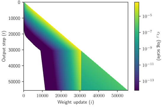
(c) Step

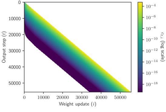
(d) Constant

Figure 27: EMA perspective: weight update contribution across steps: Convex combination of weight updates, with color indicating value of combination coefficients $c_{t,i}$: each $c_{t,i}$ gives the contribution of the $i$th update (across x-axis) to model weights $\theta_{t}$ across steps $t$ (y-axis). Note that LR schedules and coefficients corresponding to the final step only were presented earlier in Figure 2 (except for Constant). Coefficients correspond to settings for 111M-parameter models trained to 200 TPP: $t$=$55680$, $\tilde{\eta}$=$1.6\mbox{e-}02$, $\rho$=$\nicefrac{{1}}{{3}}$, $\lambda$=$0.1$.

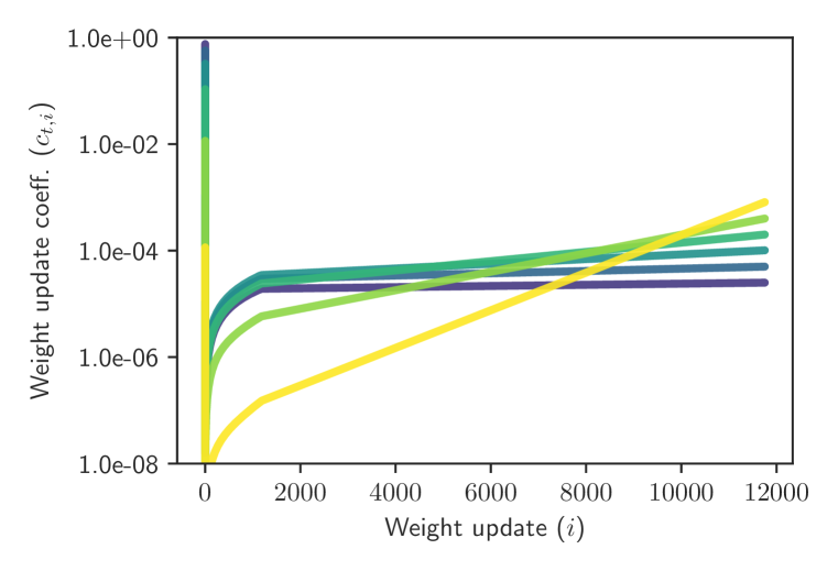
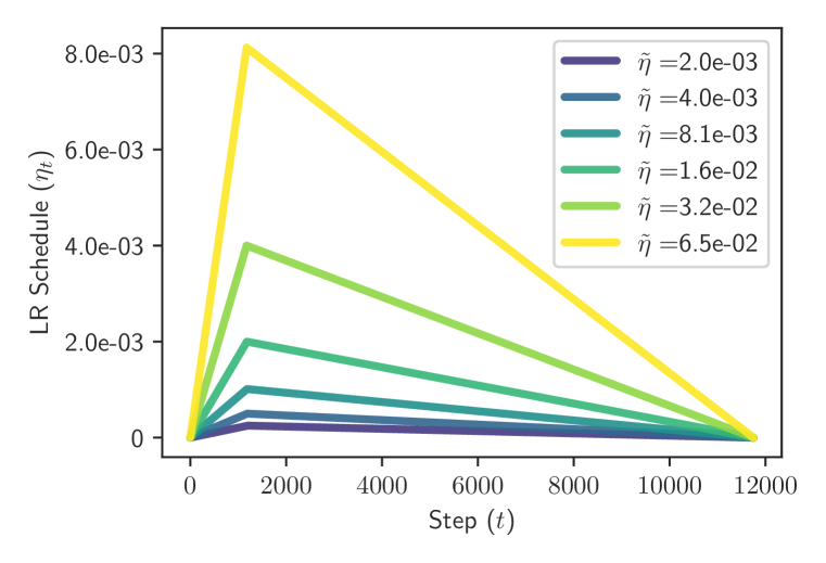
(a) Constant (b) Linear D2Z (c) InvSqrt (d) Rational

Figure 28: LR curves and dual coefficients for various common LR schedules as well as the proposed Rational approach (Section D.1): Dual coefficients shown at final training step (right side) for 610M-parameter, 20 TPP training ($t$=$11752$, $\rho$=$\nicefrac{{1}}{{8}}$, $\lambda$=$0.1$). For InvSqrt, we vary the warmup and fix $\tilde{\eta}$=$1.6\mbox{e-}02$ for all curves. Note coefficient values are plotted on log-scale

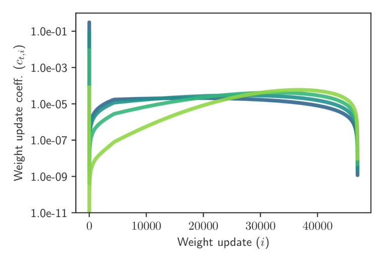
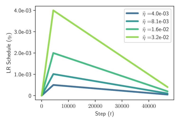
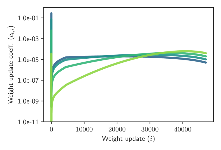
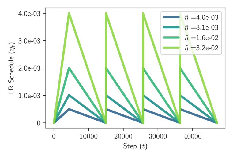
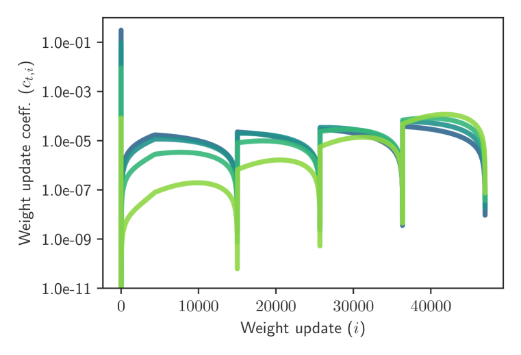
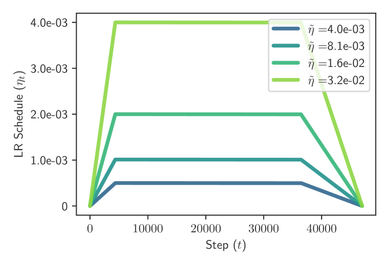
(a) Linear D2Z (b) Linear $\mbox{10}\times$ (c) Cyclic (d) WSD

Figure 29: LR curves and dual coefficients for standard vs. continuous schedules: Comparison of standard Linear schedules versus Cyclic and WSD. On the left are the exact LR schedules used in Figure 8 evaluations, i.e., 610M-parameter, 80 TPP training ($\rho$=$\nicefrac{{1}}{{8}}$, $\lambda$=$0.1$). Dual coefficients shown at at final training step $t$=$47008$ (right side). Note coefficient values are plotted on log-scale.

In this section, we provide some extra figures that were referenced in the main paper. Figure 27 shows the dual coefficients at every step of training, using color to indicate the coefficient value (log-scale). Every horizontal row/step of Figure 27 reflects the coefficients at that step, essentially providing a version of Figure 2 but at each step. Figure 28 provides the LR schedules and dual coefficients for some of the schedules discussed in the main paper, as well as our proposed Rational schedule, which combines all the prior weight updates (after warmup) equally at every step. Finally, Figure 29 gives the LR schedules and dual coefficients for the comparison to WSD and Cyclic in Figure 8.

It is worth re-iterating that the dual coefficients can be computed separately from any actual training. They are mathematically equivalent to the LR schedule itself and simply provide a perspective on how the weight updates combine to form parameters, when using the AdamW optimizer. Furthermore, it is also worth noting the vertical bar at step 1 in the dual coefficient plots; this bar reflects the coefficient on the initial, random weights. To some extent, this $c_{1,t}$ value can serve as an indicator of how far the model has moved from initial conditions, i.e., the extent to which the model has reduced the bias. In general, if $c_{1,t}$ is too high (e.g., when it outweighs the sum of the other coefficients), then bias is likely significantly hindering learning. Two effective ways to reduce $c_{1,t}$ and thus reduce bias are to (1) raise the peak LR, and (2) train for more TPP. In contrast to these two methods, raising weight decay, $\lambda$, can also decrease $c_{1,t}$, but is counterproductive for reducing bias because it also reduces the scale of weight updates, as noted in Section 3.3. Likewise, using smaller batches also reduces $c_{1,t}$, but is likewise counterproductive if the batches become too small, to the extent that gradient noise increases. However, D2Z is more robust to such noise than $\mbox{10}\times$ or Constant decay. Further investigating the interplay of $\lambda$, batch size, and peak learning rate is important future work.

References

- Aleph Alpha (2024) Aleph Alpha. Introducing Pharia-1-LLM: Transparent and compliant. Blog post, 2024. Accessed: 2024-09-07.
- Almazrouei et al. (2023) Ebtesam Almazrouei, Hamza Alobeidli, Abdulaziz Alshamsi, Alessandro Cappelli, Ruxandra Cojocaru, Mérouane Debbah, Étienne Goffinet, Daniel Hesslow, Julien Launay, Quentin Malartic, et al. The Falcon series of open language models. arXiv preprint arXiv:2311.16867, 2023.
- Andriushchenko et al. (2023) Maksym Andriushchenko, Francesco D’Angelo, Aditya Varre, and Nicolas Flammarion. Why do we need weight decay in modern deep learning? arXiv preprint arXiv:2310.04415, 2023.
- Bi et al. (2024) Xiao Bi, Deli Chen, Guanting Chen, Shanhuang Chen, Damai Dai, Chengqi Deng, Honghui Ding, Kai Dong, Qiushi Du, Zhe Fu, et al. DeepSeek LLM: Scaling open-source language models with longtermism. arXiv preprint arXiv:2401.02954, 2024.
- Biderman et al. (2023) Stella Biderman, Hailey Schoelkopf, Quentin Anthony, Herbie Bradley, Kyle O’Brien, Eric Hallahan, Mohammad Aflah Khan, Shivanshu Purohit, USVSN Sai Prashanth, Edward Raff, Aviya Skowron, Lintang Sutawika, and Oskar van der Wal. Pythia: A suite for analyzing large language models across training and scaling, 2023.
- Bjorck et al. (2024) Johan Bjorck, Alon Benhaim, Vishrav Chaudhary, Furu Wei, and Xia Song. Scaling optimal LR across token horizons. arXiv preprint arXiv:2409.19913, 2024.
- Bottou et al. (2018) Léon Bottou, Frank E Curtis, and Jorge Nocedal. Optimization methods for large-scale machine learning. SIAM review, 60(2):223–311, 2018.
- Brown et al. (2020) Tom Brown, Benjamin Mann, Nick Ryder, Melanie Subbiah, Jared D Kaplan, Prafulla Dhariwal, Arvind Neelakantan, Pranav Shyam, Girish Sastry, Amanda Askell, et al. Language models are few-shot learners. Advances in Neural Information Processing Systems, 33:1877–1901, 2020.
- Busbridge et al. (2024) Dan Busbridge, Jason Ramapuram, Pierre Ablin, Tatiana Likhomanenko, Eeshan Gunesh Dhekane, Xavier Suau Cuadros, and Russell Webb. How to scale your EMA. Advances in Neural Information Processing Systems, 36, 2024.
- Chen et al. (2016) Jianmin Chen, Xinghao Pan, Rajat Monga, Samy Bengio, and Rafal Jozefowicz. Revisiting distributed synchronous SGD. arXiv preprint arXiv:1604.00981, 2016.
- Defazio et al. (2023) Aaron Defazio, Ashok Cutkosky, Harsh Mehta, and Konstantin Mishchenko. When, why and how much? Adaptive learning rate scheduling by refinement. arXiv preprint arXiv:2310.07831, 2023.
- Defazio et al. (2024) Aaron Defazio, Harsh Mehta, Konstantin Mishchenko, Ahmed Khaled, Ashok Cutkosky, et al. The road less scheduled. arXiv preprint arXiv:2405.15682, 2024.
- Dey et al. (2023) Nolan Dey, Gurpreet Gosal, Hemant Khachane, William Marshall, Ribhu Pathria, Marvin Tom, and Joel Hestness. Cerebras-GPT: Open compute-optimal language models trained on the Cerebras wafer-scale cluster. arXiv preprint arXiv:2304.03208, 2023.
- Dey et al. (2024a) Nolan Dey, Quentin Anthony, and Joel Hestness. The practitioner’s guide to the maximal update parameterization. Blog post, 2024a.
- Dey et al. (2024b) Nolan Dey, Shane Bergsma, and Joel Hestness. Sparse maximal update parameterization: A holistic approach to sparse training dynamics. arXiv preprint arXiv:2405.15743, 2024b.
- Dubey et al. (2024) Abhimanyu Dubey, Abhinav Jauhri, Abhinav Pandey, Abhishek Kadian, Ahmad Al-Dahle, Aiesha Letman, Akhil Mathur, Alan Schelten, Amy Yang, Angela Fan, et al. The Llama 3 herd of models. arXiv preprint arXiv:2407.21783, 2024.
- Filatov et al. (2024) Oleg Filatov, Jan Ebert, Jiangtao Wang, and Stefan Kesselheim. Time transfer: On optimal learning rate and batch size in the infinite data limit. arXiv preprint arXiv:2410.05838, 2024.
- Gao et al. (2020) Leo Gao, Stella Biderman, Sid Black, Laurence Golding, Travis Hoppe, Charles Foster, Jason Phang, Horace He, Anish Thite, Noa Nabeshima, Shawn Presser, and Connor Leahy. The Pile: An 800GB dataset of diverse text for language modeling, 2020.
- Ge et al. (2019) Rong Ge, Sham M Kakade, Rahul Kidambi, and Praneeth Netrapalli. The step decay schedule: A near optimal, geometrically decaying learning rate procedure for least squares. Advances in neural information processing systems, 32, 2019.
- Glorot & Bengio (2010) Xavier Glorot and Yoshua Bengio. Understanding the difficulty of training deep feedforward neural networks. In Proceedings of the Thirteenth International Conference on Artificial Intelligence and Statistics (PMLR), 2010.
- Gokaslan & Cohen (2019) Aaron Gokaslan and Vanya Cohen. OpenWebText corpus. Web page, 2019.
- Goyal et al. (2018) Priya Goyal, Piotr Dollár, Ross Girshick, Pieter Noordhuis, Lukasz Wesolowski, Aapo Kyrola, Andrew Tulloch, Yangqing Jia, and Kaiming He. Accurate, large minibatch SGD: Training ImageNet in 1 hour, 2018.
- Graves (2013) Alex Graves. Generating sequences with recurrent neural networks. arXiv preprint arXiv:1308.0850, 2013.
- Gray et al. (2024) Gavia Gray, Aman Tiwari, Shane Bergsma, and Joel Hestness. Normalization layer per-example gradients are sufficient to predict gradient noise scale in transformers. arXiv preprint arXiv:2411.00999, 2024.
- Gupta et al. (2018) Vineet Gupta, Tomer Koren, and Yoram Singer. Shampoo: Preconditioned stochastic tensor optimization. In International Conference on Machine Learning, pp. 1842–1850. PMLR, 2018.
- Hägele et al. (2024) Alexander Hägele, Elie Bakouch, Atli Kosson, Loubna Ben Allal, Leandro Von Werra, and Martin Jaggi. Scaling laws and compute-optimal training beyond fixed training durations. arXiv preprint arXiv:2405.18392, 2024.
- He et al. (2015) Kaiming He, Xiangyu Zhang, Shaoqing Ren, and Jian Sun. Delving deep into rectifiers: Surpassing human-level performance on ImageNet classification. In Proceedings of the IEEE international conference on computer vision, pp. 1026–1034, 2015.
- He et al. (2016) Kaiming He, Xiangyu Zhang, Shaoqing Ren, and Jian Sun. Deep residual learning for image recognition. In Proceedings of the IEEE conference on computer vision and pattern recognition, pp. 770–778, 2016.
- Henighan et al. (2020) Tom Henighan, Jared Kaplan, Mor Katz, Mark Chen, Christopher Hesse, Jacob Jackson, Heewoo Jun, Tom B Brown, Prafulla Dhariwal, Scott Gray, et al. Scaling laws for autoregressive generative modeling. arXiv preprint arXiv:2010.14701, 2020.
- Hoefler et al. (2021) Torsten Hoefler, Dan Alistarh, Tal Ben-Nun, Nikoli Dryden, and Alexandra Peste. Sparsity in deep learning: Pruning and growth for efficient inference and training in neural networks. Journal of Machine Learning Research, 22(241):1–124, 2021.
- Hoffer et al. (2017) Elad Hoffer, Itay Hubara, and Daniel Soudry. Train longer, generalize better: Closing the generalization gap in large batch training of neural networks. Advances in Neural Information Processing Systems, 30, 2017.
- Hoffmann et al. (2022) Jordan Hoffmann, Sebastian Borgeaud, Arthur Mensch, Elena Buchatskaya, Trevor Cai, Eliza Rutherford, Diego de Las Casas, Lisa Anne Hendricks, Johannes Welbl, Aidan Clark, et al. An empirical analysis of compute-optimal large language model training. Advances in Neural Information Processing Systems, 35, 2022.
- Howard & Ruder (2018) Jeremy Howard and Sebastian Ruder. Universal language model fine-tuning for text classification. arXiv preprint arXiv:1801.06146, 2018.
- Hu et al. (2024) Shengding Hu, Yuge Tu, Xu Han, Chaoqun He, Ganqu Cui, Xiang Long, Zhi Zheng, Yewei Fang, Yuxiang Huang, Weilin Zhao, et al. MiniCPM: Unveiling the potential of small language models with scalable training strategies. arXiv preprint arXiv:2404.06395, 2024.
- Ibrahim et al. (2024) Adam Ibrahim, Benjamin Thérien, Kshitij Gupta, Mats L Richter, Quentin Anthony, Timothée Lesort, Eugene Belilovsky, and Irina Rish. Simple and scalable strategies to continually pre-train large language models. arXiv preprint arXiv:2403.08763, 2024.
- Kaplan et al. (2020) Jared Kaplan, Sam McCandlish, Tom Henighan, Tom B. Brown, Benjamin Chess, Rewon Child, Scott Gray, Alec Radford, Jeffrey Wu, and Dario Amodei. Scaling laws for neural language models, 2020.
- Karpathy (2024) Andrej Karpathy. nanoGPT. github.com/karpathy/nanoGPT, 2024. GitHub repository.
- Kingma & Ba (2014) Diederik P Kingma and Jimmy Ba. Adam: A method for stochastic optimization. arXiv preprint arXiv:1412.6980, 2014.
- Kosson et al. (2024) Atli Kosson, Bettina Messmer, and Martin Jaggi. Analyzing & reducing the need for learning rate warmup in GPT training. In arXiv preprint arXiv:2410.23922, 2024.
- Krizhevsky (2014) Alex Krizhevsky. One weird trick for parallelizing convolutional neural networks. arXiv preprint arXiv:1404.5997, 2014.
- Leviathan et al. (2023) Yaniv Leviathan, Matan Kalman, and Yossi Matias. Fast inference from transformers via speculative decoding. In International Conference on Machine Learning, pp. 19274–19286. PMLR, 2023.
- Li et al. (2019) Mengtian Li, Ersin Yumer, and Deva Ramanan. Budgeted training: Rethinking deep neural network training under resource constraints. arXiv preprint arXiv:1905.04753, 2019.
- Li et al. (2023) Yuanzhi Li, Sébastien Bubeck, Ronen Eldan, Allie Del Giorno, Suriya Gunasekar, and Yin Tat Lee. Textbooks are all you need II: phi-1.5 technical report. arXiv preprint arXiv:2309.05463, 2023.
- Li et al. (2020) Zhiyuan Li, Kaifeng Lyu, and Sanjeev Arora. Reconciling modern deep learning with traditional optimization analyses: The intrinsic learning rate. Advances in Neural Information Processing Systems, 33:14544–14555, 2020.
- Lingle (2024) Lucas Lingle. A large-scale exploration of -transfer. arXiv preprint arXiv:2404.05728, 2024.
- Liu et al. (2019) Liyuan Liu, Haoming Jiang, Pengcheng He, Weizhu Chen, Xiaodong Liu, Jianfeng Gao, and Jiawei Han. On the variance of the adaptive learning rate and beyond. arXiv preprint arXiv:1908.03265, 2019.
- Loshchilov & Hutter (2017) Ilya Loshchilov and Frank Hutter. Decoupled weight decay regularization. In International Conference on Learning Representations, 2017.
- Malladi et al. (2022) Sadhika Malladi, Kaifeng Lyu, Abhishek Panigrahi, and Sanjeev Arora. On the SDEs and scaling rules for adaptive gradient algorithms. Advances in Neural Information Processing Systems, 35:7697–7711, 2022.
- McCandlish et al. (2018) Sam McCandlish, Jared Kaplan, Dario Amodei, and OpenAI Dota Team. An empirical model of large-batch training, 2018.
- Mesnard et al. (2024) Thomas Mesnard, Cassidy Hardin, Robert Dadashi, Surya Bhupatiraju, Shreya Pathak, Laurent Sifre, Morgane Rivière, Mihir Sanjay Kale, Juliette Love, et al. Gemma: Open models based on gemini research and technology. arXiv preprint arXiv:2403.08295, 2024.
- Moulines & Bach (2011) Eric Moulines and Francis Bach. Non-asymptotic analysis of stochastic approximation algorithms for machine learning. Advances in Neural Information Processing Systems, 24, 2011.
- Muennighoff et al. (2023) Niklas Muennighoff, Alexander Rush, Boaz Barak, Teven Le Scao, Nouamane Tazi, Aleksandra Piktus, Sampo Pyysalo, Thomas Wolf, and Colin A Raffel. Scaling data-constrained language models. Advances in Neural Information Processing Systems, 36, 2023.
- Noci et al. (2024) Lorenzo Noci, Alexandru Meterez, Thomas Hofmann, and Antonio Orvieto. Why do learning rates transfer? Reconciling optimization and scaling limits for deep learning. arXiv preprint arXiv:2402.17457, 2024.
- Porian et al. (2024) Tomer Porian, Mitchell Wortsman, Jenia Jitsev, Ludwig Schmidt, and Yair Carmon. Resolving discrepancies in compute-optimal scaling of language models. arXiv preprint arXiv:2406.19146, 2024.
- Press et al. (2022) Ofir Press, Noah Smith, and Mike Lewis. Train short, test long: Attention with linear biases enables input length extrapolation. In International Conference on Learning Representations, 2022.
- Radford et al. (2019) Alec Radford, Jeffrey Wu, Rewon Child, David Luan, Dario Amodei, and Ilya Sutskever. Language models are unsupervised multitask learners, 2019.
- Rae et al. (2022) Jack W. Rae, Sebastian Borgeaud, Trevor Cai, Katie Millican, Jordan Hoffmann, Francis Song, John Aslanides, Sarah Henderson, Roman Ring, Susannah Young, et al. Scaling language models: Methods, analysis & insights from training Gopher, 2022.
- Raffel et al. (2020) Colin Raffel, Noam Shazeer, Adam Roberts, Katherine Lee, Sharan Narang, Michael Matena, Yanqi Zhou, Wei Li, and Peter J. Liu. Exploring the limits of transfer learning with a unified text-to-text transformer. Journal of Machine Learning Research, 2020.
- Robbins & Monro (1951) Herbert Robbins and Sutton Monro. A stochastic approximation method. The Annals of Mathematical Statistics, pp. 400–407, 1951.
- Sandler et al. (2023) Mark Sandler, Andrey Zhmoginov, Max Vladymyrov, and Nolan Miller. Training trajectories, mini-batch losses and the curious role of the learning rate. arXiv preprint arXiv:2301.02312, 2023.
- Sanyal et al. (2023) Sunny Sanyal, Atula Neerkaje, Jean Kaddour, Abhishek Kumar, and Sujay Sanghavi. Early weight averaging meets high learning rates for LLM pre-training. arXiv preprint arXiv:2306.03241, 2023.
- Scao et al. (2023) Teven Le Scao, Angela Fan, Christopher Akiki, Ellie Pavlick, Suzana Ilić, Daniel Hesslow, Roman Castagné, Alexandra Sasha Luccioni, François Yvon, Matthias Gallé, et al. BLOOM: A 176b-parameter open-access multilingual language model, 2023.
- Schmidt et al. (2021) Robin M Schmidt, Frank Schneider, and Philipp Hennig. Descending through a crowded valley-benchmarking deep learning optimizers. In International Conference on Machine Learning, pp. 9367–9376. PMLR, 2021.
- Sengupta et al. (2023) Neha Sengupta, Sunil Kumar Sahu, Bokang Jia, Satheesh Katipomu, Haonan Li, Fajri Koto, William Marshall, Gurpreet Gosal, Cynthia Liu, Zhiming Chen, et al. Jais and Jais-chat: Arabic-centric foundation and instruction-tuned open generative large language models. arXiv preprint arXiv:2308.16149, 2023.
- Shallue et al. (2019) Christopher J Shallue, Jaehoon Lee, Joseph Antognini, Jascha Sohl-Dickstein, Roy Frostig, and George E Dahl. Measuring the effects of data parallelism on neural network training. Journal of Machine Learning Research, 20(112):1–49, 2019.
- Shazeer (2020) Noam Shazeer. GLU variants improve transformer, 2020.
- Shen et al. (2024a) Yikang Shen, Zhen Guo, Tianle Cai, and Zengyi Qin. JetMoE: Reaching Llama2 performance with 0.1M dollars. arXiv preprint arXiv:2404.07413, 2024a.
- Shen et al. (2024b) Yikang Shen, Matthew Stallone, Mayank Mishra, Gaoyuan Zhang, Shawn Tan, Aditya Prasad, Adriana Meza Soria, David D Cox, and Rameswar Panda. Power scheduler: A batch size and token number agnostic learning rate scheduler. arXiv preprint arXiv:2408.13359, 2024b.
- Smith (2017) Leslie N Smith. Cyclical learning rates for training neural networks. In 2017 IEEE Winter Conference on Applications of Computer Vision (WACV), pp. 464–472. IEEE, 2017.
- Smith et al. (2018) Samuel L. Smith, Pieter-Jan Kindermans, and Quoc V. Le. Don’t decay the learning rate, increase the batch size. In International Conference on Learning Representations, 2018.
- Soboleva et al. (2023) Daria Soboleva, Faisal Al-Khateeb, Robert Myers, Jacob R Steeves, Joel Hestness, and Nolan Dey. SlimPajama: A 627B token cleaned and deduplicated version of RedPajama. Blog post, 2023.
- Tissue et al. (2024) Howe Tissue, Venus Wang, and Lu Wang. Scaling law with learning rate annealing. arXiv preprint arXiv:2408.11029, 2024.
- Touvron et al. (2023a) Hugo Touvron, Thibaut Lavril, Gautier Izacard, Xavier Martinet, Marie-Anne Lachaux, Timothée Lacroix, Baptiste Rozière, Naman Goyal, Eric Hambro, Faisal Azhar, Aurelien Rodriguez, Armand Joulin, Edouard Grave, and Guillaume Lample. LLaMA: Open and efficient foundation language models, 2023a.
- Touvron et al. (2023b) Hugo Touvron, Louis Martin, Kevin Stone, Peter Albert, Amjad Almahairi, Yasmine Babaei, Nikolay Bashlykov, Soumya Batra, Prajjwal Bhargava, Shruti Bhosale, et al. LLaMA 2: Open foundation and fine-tuned chat models. arXiv preprint arXiv:2307.09288, 2023b.
- Vaswani et al. (2017) Ashish Vaswani, Noam Shazeer, Niki Parmar, Jakob Uszkoreit, Llion Jones, Aidan N Gomez, Łukasz Kaiser, and Illia Polosukhin. Attention is all you need. In Advances in Neural Information Processing Systems, 2017.
- Wang & Aitchison (2024) Xi Wang and Laurence Aitchison. How to set AdamW’s weight decay as you scale model and dataset size. arXiv preprint arXiv:2405.13698, 2024.
- Wortsman et al. (2023) Mitchell Wortsman, Peter J Liu, Lechao Xiao, Katie Everett, Alex Alemi, Ben Adlam, John D Co-Reyes, Izzeddin Gur, Abhishek Kumar, Roman Novak, et al. Small-scale proxies for large-scale transformer training instabilities. arXiv preprint arXiv:2309.14322, 2023.
- Xing et al. (2018) Chen Xing, Devansh Arpit, Christos Tsirigotis, and Yoshua Bengio. A walk with SGD. arXiv preprint arXiv:1802.08770, 2018.
- Xiong et al. (2020) Ruibin Xiong, Yunchang Yang, Di He, Kai Zheng, Shuxin Zheng, Chen Xing, Huishuai Zhang, Yanyan Lan, Liwei Wang, and Tieyan Liu. On layer normalization in the transformer architecture. In International Conference on Machine Learning, pp. 10524–10533. PMLR, 2020.
- Yang & Hu (2020) Greg Yang and Edward J Hu. Feature learning in infinite-width neural networks. arXiv preprint arXiv:2011.14522, 2020.
- Yang et al. (2021) Greg Yang, Edward Hu, Igor Babuschkin, Szymon Sidor, Xiaodong Liu, David Farhi, Nick Ryder, Jakub Pachocki, Weizhu Chen, and Jianfeng Gao. Tuning large neural networks via zero-shot hyperparameter transfer. In Advances in Neural Information Processing Systems, 2021.
- You et al. (2019a) Kaichao You, Mingsheng Long, Jianmin Wang, and Michael I Jordan. How does learning rate decay help modern neural networks? arXiv preprint arXiv:1908.01878, 2019a.
- You et al. (2019b) Yang You, Jing Li, Sashank Reddi, Jonathan Hseu, Sanjiv Kumar, Srinadh Bhojanapalli, Xiaodan Song, James Demmel, Kurt Keutzer, and Cho-Jui Hsieh. Large batch optimization for deep learning: Training BERT in 76 minutes. arXiv preprint arXiv:1904.00962, 2019b.
- Zagoruyko & Komodakis (2016) Sergey Zagoruyko and Nikos Komodakis. Wide residual networks. arXiv preprint arXiv:1605.07146, 2016.
- Zhai et al. (2022) Xiaohua Zhai, Alexander Kolesnikov, Neil Houlsby, and Lucas Beyer. Scaling vision transformers. In Proceedings of the IEEE/CVF conference on computer vision and pattern recognition, pp. 12104–12113, 2022.
- Zhang et al. (2024) Hanlin Zhang, Depen Morwani, Nikhil Vyas, Jingfeng Wu, Difan Zou, Udaya Ghai, Dean Foster, and Sham Kakade. How does critical batch size scale in pre-training? arXiv preprint arXiv:2410.21676, 2024.