Modal analysis of a domain decomposition method for Maxwell’s equations in a waveguide

Abstract

Time-harmonic wave propagation problems, especially those governed by Maxwell’s equations, pose significant computational challenges due to the non-self-adjoint nature of the operators and the large, non-Hermitian linear systems resulting from discretization. Domain decomposition methods, particularly one-level Schwarz methods, offer a promising framework to tackle these challenges, with recent advancements showing the potential for weak scalability under certain conditions. In this paper, we analyze the weak scalability of one-level Schwarz methods for Maxwell’s equations in strip-wise domain decompositions, focusing on waveguides with general cross sections and different types of transmission conditions such as impedance or perfectly matched layers (PMLs). By combining techniques from the limiting spectrum analysis of Toeplitz matrices and the modal decomposition of Maxwell’s solutions, we provide a novel theoretical framework that extends previous work to more complex geometries and transmission conditions. Numerical experiments confirm that the limiting spectrum effectively predicts practical behavior even with a modest number of subdomains. Furthermore, we demonstrate that the one-level Schwarz method can achieve robustness with respect to the wave number under specific domain decomposition parameters, offering new insights into its applicability for large-scale electromagnetic wave problems.

to be added

1 Introduction

Time-harmonic wave propagation problems, particularly those arising in electromagnetic applications governed by Maxwell’s equations, present significant computational challenges. At the continuous level, these problems involve non-self-adjoint operators when impedance boundary conditions are imposed. When discretized, the number of degrees of freedom must grow with the wave number to mitigate the pollution effect, meaning that the numerical wave speed deviates from the exact solution [1]. This increase in discretization leads to large-scale, non-Hermitian linear systems that are difficult to solve using traditional iterative methods.

Over the past two decades, significant advances have been made in developing efficient solvers and preconditioners for these problems. Among these approaches, domain decomposition methods [14] offer an effective balance between direct and iterative strategies. Enhanced domain decomposition techniques, such as those using optimized transmission conditions, have proven successful for Helmholtz equations [17] and their extensions to Maxwell’s equations [13, 11, 16] and elastic wave problems [6, 23]. For large-scale problems, robustness in terms of subdomain count and wave number has been achieved by introducing two-level methods that leverage absorptive counterparts of the equations as preconditioners, solved iteratively using domain decomposition techniques [2, 15, 19].

More recently, an intriguing concept has emerged: achieving weak scalability with one-level Schwarz methods under certain conditions on the problem’s physical and numerical parameters, such as absorption and subdomain size. This ensures that the convergence rate remains stable as the number of subdomains increases, enabling the solution of increasingly complex problems without requiring a coarse space [18, 20]. Unlike traditional scalability that pertains to a fixed problem, weak scalability applies to a family of problems, where increasing the number of subdomains facilitates the solution of more challenging instances while maintaining consistent convergence rates. This concept has been explored in computational chemistry [7] and analyzed rigorously using Fourier techniques [8]. Extensions of this work to broader geometries and one-level methods have been achieved through variational and propagation-tracking analyses [9]. Such analyses have been generalized only later to complex valued problems, decompositions into multiple subdomains and optimisation of transmission conditions in [12, 15].

Notably in [4] authors investigates the convergence properties of one-level parallel Schwarz methods with Robin transmission conditions for time-harmonic wave problems, focusing on 1D and 2D Helmholtz and 2D Maxwell equations. By utilizing the block Toeplitz structure of the Schwarz iteration matrix, the authors provide a novel analysis of the limiting spectrum, showing that weak scalability can be achieved without a coarse space under specific conditions, particularly in strip-wise decompositions commonly found in waveguide problems. Building on these ideas, in this work, we examine the weak scalability of one-level methods for Maxwell’s equations in the context of strip-wise domain decompositions, as these naturally arise in waveguide problems of general cross section and with more general transmission conditions. While previous studies focused on wave number robustness [18, 20], our emphasis is on scalability over a growing chain of subdomains with fixed size, independent of discretisation. This approach provides new insights into the efficiency and applicability of domain decomposition methods for large-scale electromagnetic wave problems. The main difficulty for Maxwell’s equations resides in the vector nature of the problem and the analysis will be facilitated by the modal decomposition into Transverse Electric (TE) and Transverse Magnetic (TM) modes like in [13].

The main contributions of this paper are:

• We analyze the limiting spectrum of a one-level Schwarz method applied to strip-wise domain decompositions for Maxwell’s equations in a waveguide of a general cross section.

• Our analysis, conducted at the continuous level, is valid for a more general class of transmission conditions like impedance or perfectly matched layers (PMLs) and this analysis relies on a combination of limiting spectrum of Toeplitz matrices, introduced in [4] and the modal decompositions of the Maxwell’s solutions like in [13].

• Numerical experiments demonstrate that again limiting spectrum is highly predictive of practical behavior, even for relatively few subdomains.

• We will also show that, under specific domain decomposition parameters, in addition to scalability, the one-level Schwarz method can also achieve robustness with respect of the wavenumber.

The structure of the paper is as follows: in Section 2 we recall elements of modal analysis for Maxwell’s equations in a waveguide of general cross sections. In Section 3 we present and analyse the domain decomposition method with different types of transmission conditions relying on the modal decomposition and limiting spectrum. Finally in Section 4 we present two types of numerical results: first, showing that the limiting spectrum is descriptive for the convergence of the algorithm even in the case of a moderate number of domains and then on the discretised problem using the edge element method.

2 Modal decomposition in a waveguide

Let us consider the classical Maxwell’s equation in time-harmonic regime in the first and second order form (with convention $e^{-\imath\omega t}$ where $\omega$ is the pulsation):

(1) $$\left\{\begin{array}[]{lll}\nabla\times{\mathbf{E}}=\imath\omega\mu{\mathbf{H}}&\text{in}&\Omega,\\ \nabla\times{\mathbf{H}}=-\imath\omega\varepsilon{\mathbf{E}}&\text{in}&\Omega,\\ {\mathbf{E}}\times\mathbf{n}=\mathbf{0}.&\text{on}&\partial\Omega.\end{array}\right.\quad\Leftrightarrow\quad\left\{\begin{array}[]{lll}\nabla\times\nabla\times{\mathbf{E}}-k^{2}{\mathbf{E}}=0&\text{in}&\Omega,\\ {\mathbf{E}}\times\mathbf{n}=\mathbf{0}.&\text{on}&\partial\Omega,\end{array}\right.$$

where we denote by $k^{2}=\varepsilon\mu\omega^{2}$ the wavenumber, by $\varepsilon=\varepsilon^{\prime}-\imath\varepsilon^{\prime\prime}$ the (complex) electric permittivity and $\mu$ the magnetic permeability. The unknown vector functions are respectively the electric ${\mathbf{E}}$ and magnetic fields ${\mathbf{H}}$. All physical parameters are assumed to be constant in what follows. Although we will work mainly on the second-order formulation, the first-order formulation will be useful later, this is why it is also introduced here.

The domain $\Omega$ is a straight infinite waveguide of geometry $\mathbb{R}\times S$ where $S$ denotes the section of the waveguide, see the example Figure 1. On the boundaries, we consider Perfect Electric Conductor (PEC) conditions ($\mathbf{E}\times\mathbf{n}=0$) and $\mathbf{n}$ denotes the outward normal. The purpose of this section is illustrate the computation of solutions of Maxwell’s equations in this type of geometry which relies on the modal decomposition of the electric field. We will follow the presentation given in [10].

We call modes particular solutions of the Maxwell equations of the form

$${\mathbf{E}}=e^{\imath\beta x}\widehat{\bf{E}}(y,z)\quad\text{and}\quad{\mathbf{H}}=e^{\imath\beta x}\widehat{\bf{H}}(y,z),$$

where $\beta$ is a complex number whose meaning will be explained later and $\widehat{\bf{E}}$, $\widehat{\bf{H}}$ are vector valued fields defined in the cross section.

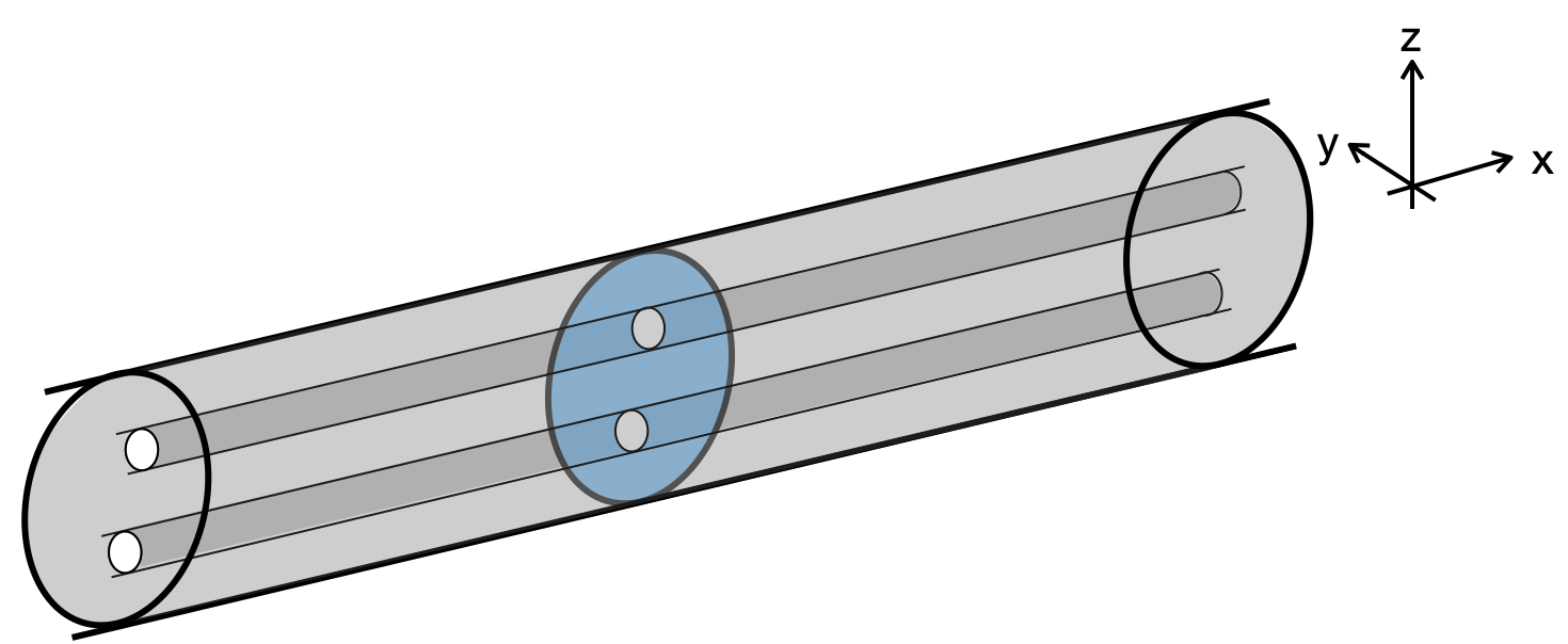
Figure 1: Scheme of the geometry $\Omega$. In blue, cross-sections of the waveguide.

In what follows we will give an overview of different case scenarios that could appear when the modes are solutions to the Maxwell’s equations.

From the second equation of the Maxwell system (1) written in the first order form, we can easily see that the electric field ${\mathbf{E}}$ is divergence free so that $\nabla\cdot{\mathbf{E}}=0$. As a consequence, using the fact that $\nabla\times\nabla\times=\nabla\left(\nabla\cdot\right)-\mathbf{\Delta}$, we get that each component of ${\mathbf{E}}$ satisfies a scalar Helmholtz equation:

(2) $$-\Delta E_{i}-k^{2}E_{i}=0\quad\text{in}\quad\Omega,\quad\forall i\in\{x,y,z\}.$$

Now, for the boundary conditions we have:

(3) $${\mathbf{E}}\times\mathbf{n}=\mathbf{0}\;\; \Leftrightarrow\;\;\left[\begin{matrix}E_{x}\\ E_{y}\\ E_{z}\end{matrix}\right]\times\left[\begin{matrix}0\\ n_{y}\\ n_{z}\end{matrix}\right]\;\;\Leftrightarrow\;\;\left[\begin{matrix}E_{y}n_{z}-E_{z}n_{y}\\ -E_{x}n_{z}\\ E_{x}n_{y}\end{matrix}\right]=\left[\begin{matrix}0\\ 0\\ 0\end{matrix}\right]$$

(6) $$\Leftrightarrow\;\;\begin{array}[]{|lll}E_{y}n_{z}-E_{z}n_{y}=0&\text{on}&\mathbb{R}\times\partial S,\\ E_{x}=0&\text{on}&\mathbb{R}\times\partial S.\end{array}$$

In particular, we deduce that $\widehat{E}_{x}$ in $E_{x}=e^{\imath\beta x}\widehat{E}_{x}(y,z)$ satisfies

(7) $$\begin{array}[]{|lll}-\Delta_{(y,z)}\widehat{E}_{x}-\left(k^{2}-\beta^{2}\right)\widehat{E}_{x}=0&\text{in}&S,\\ \widehat{E}_{x}=0&\text{on}&\partial S.\end{array}$$

where $\Delta_{(y,z)}$ denotes the Laplace operator in the two-dimensional cross section. Following the same reasoning and using the second order formulation for ${\mathbf{H}}$, we can show that $\widehat{H}_{x}$ satisfies

(8) $$\begin{array}[]{|lll}-\Delta_{(y,z)}\widehat{H}_{x}-\left(k^{2}-\beta^{2}\right)\widehat{H}_{x}=0&\text{in}&S,\\ \partial_{\mathbf{n}}\widehat{H}_{x}=0&\text{on}&\partial S.\end{array}$$

Note that knowing $\widehat{E}_{x}$ and $\widehat{H}_{x}$ one can reconstruct the full vector fields $\widehat{{\mathbf{E}}}$ and $\widehat{{\mathbf{H}}}$. Indeed, from the first order formulation of the Maxwell equations, we have:

(9) $$\begin{array}[]{|lll}\partial_{y}\widehat{E}_{z}-\partial_{z}\widehat{E}_{y}=\imath\omega\mu\widehat{H}_{x},\\ -\imath\beta\widehat{E}_{z}+\partial_{z}\widehat{E}_{x}=\imath\omega\mu\widehat{H}_{y},\\ \imath\beta\widehat{E}_{y}-\partial_{y}\widehat{E}_{x}=\imath\omega\mu\widehat{H}_{z},\end{array}\quad\text{and}\quad\begin{array}[]{|lll}\partial_{y}\widehat{H}_{z}-\partial_{z}\widehat{H}_{y}=-(\imath\omega\varepsilon-\sigma)\widehat{E}_{x},\\ -\imath\beta\widehat{H}_{z}+\partial_{z}\widehat{H}_{x}=-(\imath\omega\varepsilon-\sigma)\widehat{E}_{y},\\ \imath\beta\widehat{H}_{y}-\partial_{y}\widehat{H}_{x}=-(\imath\omega\varepsilon-\sigma)\widehat{E}_{z},\end{array}$$

Taking now the last two equations of both systems, we get that

(10) $$\left[\begin{matrix}-(\imath\omega\varepsilon-\sigma)&0&0&\imath\beta\\ 0&-(\imath\omega\varepsilon-\sigma)&-\imath\beta&0\\ 0&\imath\beta&\imath\omega\mu&0\\ -\imath\beta&0&0&\imath\omega\mu\\ \end{matrix}\right]\left[\begin{matrix}\widehat{E}_{y}\\ \widehat{E}_{z}\\ \widehat{H}_{y}\\ \widehat{H}_{z}\end{matrix}\right]=\left[\begin{matrix}\partial_{z}\widehat{H}_{x}\\ -\partial_{y}\widehat{H}_{x}\\ \partial_{z}\widehat{E}_{x}\\ -\partial_{y}\widehat{E}_{x}\end{matrix}\right].$$

We can easily see that that the determinant of the matrix is not zero iff $k^{2}-\beta^{2}\neq 0$ and in this case the components $(\widehat{E}_{y},\widehat{E}_{z})$ and $(\widehat{H}_{y},\widehat{H}_{z})$ are uniquely defined.

Depending on the values of $\widehat{E}_{x}$ and $\widehat{H}_{x}$ will distinguish now between three case scenarios allowing us to identify different types of modes corresponding to different types of particular solutions of Maxwell’s equations in the waveguide.

Transverse Electric (TE) modes: $\widehat{E}_{x}=0$ and $\widehat{H}_{x}\neq 0$

In this case since $\widehat{H}_{x}$ is solution to Equation 8, we deduce $\widehat{H}_{x}$ is a linear combination of the functions:

$$e^{\imath m\beta_{i}^{\rm TE}x}\varphi^{\mathcal{N}}_{i}(y,z)\quad\text{where}\quad\beta^{\rm TE}_{i}=\sqrt{k^{2}-(\lambda^{\mathcal{N}})^{2}_{i}},\;\;i\in\mathbb{N}^{+},\;\;m\in\{-,+\},$$

and

(11) $$\begin{array}[]{|lll}-\Delta_{(y,z)}\varphi^{\mathcal{N}}=\lambda^{\mathcal{N}}\varphi^{\mathcal{N}}&\text{in}&S,\\[5.0pt] \partial_{\mathbf{n}}\varphi^{\mathcal{N}}=0&\text{on}&\partial S.\end{array}$$

The coefficients of the decomposition that we will denote by $A_{i}^{{\rm TE},m}$ are called modal amplitudes and the sign $m$ indicates the direction of propagation of the mode, $m=+$ corresponding to right-going modes (propagating toward $+\infty$) and $m=-$ corresponding to left-going modes (propagating toward $-\infty$).

Classically, when $\beta^{\rm TE}_{i}$ is real we say that the mode is propagative and when Im$\left(\beta^{\rm TE}_{i}\right)\neq 0$ we say that the mode is evanescent.

Remark 2.1.

We remind that the eigenvalue problem (11) has an infinite countable set of solutions with $(\lambda^{\mathcal{N}}_{i})_{i\in\mathbb{N}}$ an increasing positive sequence that tends to $+\infty$ and the set of eigenfunctions $(\varphi^{\mathcal{N}}_{i})_{i\in\mathbb{N}}$ is an orthonormal basis of $L^{2}(S)$. Let us emphasize that for the first mode corresponding to $i=0$ and $\varphi_{0}=1$, the associated modal amplitude $A^{{\rm TE},m}_{i}=0$. Indeed, using the first equation of (9) of the left system, we get that:

$$\imath\omega\int_{S}\widehat{H}_{x}dS=\int_{S}\partial_{y}\widehat{E}_{z}-\partial_{z}\widehat{E}_{y}dS=\int_{\partial S}\widehat{E}_{z}n_{y}-\widehat{E}_{y}n_{z}=0,$$

according to the BC satisfied by ${\mathbf{E}}$. Then, we can deduce using the orthogonality of the eigenfunctions $\varphi^{\mathcal{N}}_{j}$ that necessarily $A^{TE,m}_{0}=0$ because

$$A^{{\rm TE},m}_{0}=\int_{S}\widehat{H}_{x}\;\varphi^{\mathcal{N}}_{0}dS=0.$$

Tranverse Magnetic modes (TM): $\widehat{E}_{x}\neq 0$ and $\widehat{H}_{x}=0$

Using a similar reasoning to the case of the TE modes, we find that $\widehat{E}_{x}$ is a linear combination of

$$e^{\imath m\beta_{i}^{\rm TM}x}\varphi^{\mathcal{D}}_{i}(y,z)\quad\text{where}\quad\beta^{\rm TM}_{i}=\sqrt{k^{2}-(\lambda^{\mathcal{D}})^{2}_{i}},\;\;i\in\mathbb{N}^{+},\;\;m\in\{-,+\},$$

and

$$\begin{array}[]{|lll}-\Delta_{y,z}\varphi^{\mathcal{D}}=\lambda^{\mathcal{D}}\varphi^{\mathcal{D}}&\text{in}&S,\\ \varphi^{\mathcal{D}}=0&\text{on}&\partial S.\end{array}$$

Here again, the above eigenvalue problem has an infinite countable set of solutions with $(\lambda^{D}_{i})_{i\in\mathbb{N}^{+}}$ an increasing positive sequence that tends to $+\infty$ and the eigenfunctions $(\varphi^{\mathcal{D}}_{i})_{i\in\mathbb{N}^{+}}$ form an orthonormal basis of $L^{2}(S)$.

Like in the case of TE-modes, we say that the mode is propagative if Im$\left(\beta^{\rm TM}_{i}\right)=0$ and evanescent if not, and the direction of propagation is given by $m$.

Transverse Electric Magnetic (TEM): $\widehat{E}_{x}=\widehat{H}_{x}=0$

Since the right hand side of Equation 10 is zero, to get non-zero solutions, we necessarily need to have $(\beta^{\rm TEM})^{2}=k^{2}$. We can show that there exist $N_{C}-1$ TEM modes where $N_{C}$ is the number of connected components of $\partial S$, see [10] for details. In particular, in the case of a waveguide with ”no holes”, there is no TEM mode propagating in the guide.

To summarise, the solutions of the Maxwell equations in a waveguide can be written as linear combination of these three types of modes:

(12) $$\begin{split}{\mathbf{E}}=&\sum_{i\geq 0}\sum_{m\in\{-,+\}}A^{{\rm TE},m}_{i}e^{\imath m\beta_{i}^{\rm TE}x}\;\widehat{{\mathbf{E}}}^{{\rm TE},m}_{i}+A^{{\rm TM},m}_{i}e^{\imath m\beta_{i}^{\rm TM}x}\;\widehat{{\mathbf{E}}}^{{\rm TM},m}_{i}\\ &+\sum_{i=1}^{N_{C}-1}\sum_{m\in\{-,+\}}A^{{\rm TEM},m}_{i}e^{\imath mkx}\widehat{{\mathbf{E}}}^{{\rm TEM},m}_{i},\end{split}$$

where the vector fields $\widehat{{\mathbf{E}}}^{{\rm TE},m}_{i}$, $\widehat{{\mathbf{E}}}^{{\rm TM},m}_{i}$ and $\widehat{{\mathbf{E}}}^{{\rm TEM},m}_{i}$ (depending on $y,z$ and defined in the section $S$) are called mode profiles, and $A^{{\rm TE},\pm}_{i}$, $A^{{\rm TM},\pm}_{i}$ and $A^{{\rm TEM},\pm}_{i}$ are the modal amplitudes associated to each type of mode. We remind that the mode profiles for TE and TM modes are determined using Equation 10 once we know $\widehat{E}_{x}$ and $\widehat{H}_{x}$ for each type of modes.

Remark 2.2.

Let us note that the TEM-modes are necessarily propagative (unlike the TE and TM modes which can be either propagative or evanescent). Also, in what follows, we will assume that we are not on a cut-off frequency $k$, that is to say a frequency s.t. there exists $i$ s.t. $\beta^{\rm TE}_{i}=0$ or $\beta^{\rm TM}_{i}=0$.

The following property regarding the continuity of the tangential traces of mode profiles will be useful later and help to manipulate Equation 12 in the underlying computations.

Proposition 2.3 (Tangential traces of mode profiles).

For $\mathbf{n}=(1,0,0)^{t}$, we can choose the mode profiles such that

$$\widehat{{\mathbf{E}}}^{\rm TE,+}_{i}\times\mathbf{n}=\widehat{{\mathbf{E}}}^{\rm TE,-}_{i}\times\mathbf{n},\quad\widehat{{\mathbf{E}}}^{\rm TM,+}_{i}\times\mathbf{n}=\widehat{{\mathbf{E}}}^{\rm TM,-}_{i}\times\mathbf{n}\quad\forall i\in\mathbb{N}^{+},$$

and

$$\widehat{{\mathbf{E}}}^{\rm TEM,+}_{i}\times\mathbf{n}=\widehat{{\mathbf{E}}}^{\rm TEM,-}_{i}\times\mathbf{n},\quad\forall i\in\{1,\cdots,N_{C}-1\}.$$

Proof 2.4.

To prove this result, let us first remark that for any field $\mathbf{U}$ we have:

(13) $$\mathbf{U}\times\mathbf{n}=\left[\begin{matrix}0\\ U_{z}\\ -U_{y}\end{matrix}\right].$$

For TE-modes, using Equation 9 and the fact that $E_{x}=\widehat{E}_{x}=0$, we deduce that

$$\widehat{E}_{y}=\dfrac{\imath\omega\mu\partial_{z}\varphi^{\mathcal{N}}_{i}}{\lambda^{\mathcal{N}}_{i}}\quad\text{and}\quad\widehat{E}_{z}=-\dfrac{\imath\omega\mu\partial_{y}\varphi^{\mathcal{N}}_{i}}{\lambda^{\mathcal{N}}_{i}}.$$

Since the expression above is independent of the sign of $\beta$ we get the first result by choosing the TE-modes profile:

$$\widehat{{\mathbf{E}}}^{\rm TE,\pm}_{i}=\left[\begin{matrix}0\\ \widehat{E}_{y}\\ \widehat{E}_{z}\end{matrix}\right].$$

A similar result holds for the TEM-modes.

Regarding the TM-modes, we use again Equation 9 and the fact that $H_{x}=\widehat{H}_{x}=0$, which leads to:

$$\widehat{E}_{y}=\dfrac{\imath\beta^{\rm TM}_{i}\partial_{y}\varphi^{\mathcal{D}}_{i}}{\lambda^{\mathcal{D}}_{i}}\quad\text{and}\quad\widehat{E}_{z}=\dfrac{\imath\beta^{\rm TM}_{i}\partial_{z}\varphi^{\mathcal{D}}_{i}}{\lambda^{\mathcal{D}}_{i}}.$$

This time, the expression does depend on the sign of $\beta$. Yet, since modes are solutions to the eigenvalues problem, the profiles $\widehat{{\mathbf{E}}}^{\rm TM,\pm}_{i}$ are defined up to a (non-zero) multiplicative constant. As a consequence, we can choose

$$\widehat{{\mathbf{E}}}^{\rm TM,+}_{i}=\left[\begin{matrix}\widehat{E}^{\rm TM,+}_{x}\\ \widehat{E}_{y}\\ \widehat{E}_{z}\end{matrix}\right]\quad\text{and}\quad\widehat{{\mathbf{E}}}^{\rm TM,-}_{i}=\left[\begin{matrix}\widehat{E}^{\rm TM,-}_{x}\\ \widehat{E}_{y}\\ \widehat{E}_{z}\end{matrix}\right],$$

which proves our result using Equation 13.

Remark 2.5.

Since for TE-modes and TEM-modes $E_{x}=0$, we could drop the exponent $\pm$ in the profile because $\widehat{{\mathbf{E}}}^{\rm TE,+}_{i}=\widehat{{\mathbf{E}}}^{\rm TE,-}_{i}$.

3 Domain decomposition algorithm

The modal analysis in Section 2 holds in the case of infinite waveguide. In what follows, for computational reasons we will truncate this waveguide to $\tilde{\Omega}=[a,b]\times S$ and add appropriate boundary conditions at the ending cross-sections $\{a\}\times S$ and $\{b\}\times S$.

To define the Schwarz algorithm, we will split this computational domain into several overlapping subdomains. Let us consider $(a_{l})_{l}$ and $(b_{l})_{l}$ s.t. $a_{1}=a$, $b_{N}=b$:

(14) $$b_{l-1}-a_{l}=\delta>0,\quad\text{and}\quad b_{l}-a_{l}=L+2\delta\quad\;\;\forall l\in\{1,\cdots,N\},$$

with $N\in\mathbb{N}$ given and $L>0$. We define by $\Omega_{l}$ the subdomain $\Omega_{l}:=[a_{l},b_{l}]\times S$ of the whole domain $\widetilde{\Omega}=\cup_{l=1}^{N}\Omega_{l}=[a_{1},b_{N}]\times S$ see Figure 2 (where we note that all subdomains are prisms with the same type of cross-section). We denote by $\delta>0$ the size of the overlapping area between two consecutive subdomains $\Omega_{l}$ and $\Omega_{l\pm 1}$.

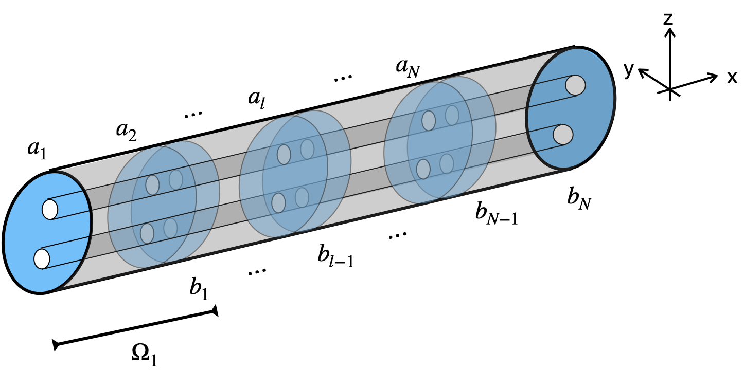
Figure 2: A bounded waveguide $\widetilde{\Omega}$ and its decomposition into subdomains.

Definition 3.1 (The Schwarz algorithm).

Let $\mathcal{L}$ be the linear second order Maxwell’s operator

(15) $$\mathcal{L}(\mathbf{E}):=\nabla\times\nabla\times\mathbf{E}-k^{2}\mathbf{E},$$

and $\mathcal{B}$ the boundary operator:

(16) $$\mathcal{B}(\mathbf{E}):=\left(\left(\nabla\times\mathbf{E}\right)\times\mathbf{n}\right)\times\mathbf{n}+\mathcal{T}(\mathbf{E}\times\mathbf{n}).$$

where $\mathcal{T}$ is a linear transmission operator which will be defined later. Starting from an initial guess, the classical Schwarz algorithm computes at iteration $n\in\mathbb{N}$ the solution in the subdomain $\Omega_{l}$ as follows

(17) $$\begin{array}[]{|lcl}\mathcal{L}(\mathbf{E}^{n,l})=\mathbf{f}_{l}&\text{in}&\Omega_{j},\\ \mathcal{B}(\mathbf{E}^{n,l})=\mathcal{B}({\mathbf{E}}^{n-1,l-1})&\text{on}&\Gamma_{l,l-1}:=\{x=a_{l}\}\times S,\\ \mathcal{B}(\mathbf{E}^{n,l})=\mathcal{B}({\mathbf{E}}^{n-1,l+1})&\text{on}&\Gamma_{l,l+1}:=\{x=b_{l}\}\times S,\\ \mathbf{E}^{n,l}\times\mathbf{n}=0&\text{on}&\partial\Omega_{l}\setminus\left(\Gamma_{l,l-1}\cup\Gamma_{l,l+1}\right).\end{array}$$

For simplicity, we will consider that boundary conditions at the extremities of the waveguide are: $\mathcal{B}(\mathbf{E}^{n-1,1})=\mathbf{g}_{1}$ and $\mathcal{B}(\mathbf{E}^{n-1,N})=\mathbf{g}_{N}$.

Remark 3.2.

Typically, if the transmission operator in Equation 16 is $\mathcal{T}=-\imath k$, then ${\cal B}$ corresponds to zero order absorbing boundary conditions that we can classically use when truncating an unbounded waveguide. This condition (roughly) takes into account what happens in the exterior domain and ensures the solution in the truncated domain is a good approximation to the restriction of the solution in the unbounded one, by ”absorbing” outgoing waves and avoiding reflections, see for instance [21, 22] for more details. Note also that for diffraction problems, these boundary conditions on $\Gamma_{1,0}$ and $\Gamma_{N,N+1}$ are usually inhomogeneous i.e. $\mathbf{g}_{1,N}\neq 0$ (if we work with the total field, i.e. the sum of the incident field and the diffracted field).

In the analysis of the algorithm below we will consider the homogeneous case (where $\mathbf{f}_{l}=\mathbf{g}_{1,N}=0$) because we will be interested the evolution of the error throughout the iterations. The convergence factor of algorithm (17) will be computed using a Fourier analysis and different types of transmissions conditions will be considered. This analysis relies on several ingredients including the modal decomposition of the waveguide solution which will allow analytical computations of the action of the transmission operators from Equation 16. In particular we will see that these operators are diagonalized by the different modes (see also the analysis in [13]).

Proposition 3.3 (Diagonalization of ${\mathbf{E}}\rightarrow((\nabla\times{\mathbf{E}})\times\mathbf{n})\times\mathbf{n}$).

Let $\mathbf{n}=(1,0,0)^{t}$ the outward normal to the waveguide cross-section. Then the operator ${\mathbf{E}}\rightarrow((\nabla\times{\mathbf{E}})\times\mathbf{n})\times\mathbf{n}$ is diagonalized by the TE, TM and TEM modes i.e. the following identities hold:
For TE-modes, we have $\forall i\in\mathbb{N}^{+}$:

(18) $$((\nabla\times\mathbf{E}^{\rm TE,\pm}_{i})\times\mathbf{n})\times\mathbf{n}=\pm\imath\beta^{\rm TE}_{i}\mathbf{E}^{\rm TE,\pm}_{i}\times\mathbf{n}\text{ where }\mathbf{E}^{\rm TE,\pm}_{i}:=\widehat{\mathbf{E}}^{\rm TE,\pm}_{i}e^{\pm\imath\beta^{\rm TE}_{i}x}.$$

For the TM-modes, we have $\forall i\in\mathbb{N}^{+}$:

(19) $$((\nabla\times\mathbf{E}^{\rm TM,\pm}_{i})\times\mathbf{n})\times\mathbf{n}=\pm\imath\dfrac{k^{2}}{\beta^{\rm TM}_{i}}\mathbf{E}^{\rm TM,\pm}_{i}\times\mathbf{n}\text{ where }\mathbf{E}^{\rm TM,\pm}_{i}:=\widehat{\mathbf{E}}^{\rm TM,\pm}_{i}e^{\pm\imath\beta^{\rm TM}_{i}x}.$$

For the TEM-modes, we have $\forall i\in\{1,\cdots N_{C}-1\}$:

(20) $$((\nabla\times\mathbf{E}^{\rm TEM,\pm}_{i})\times\mathbf{n})\times\mathbf{n}=\pm\imath k\mathbf{E}^{\rm TEM,\pm}_{i}\times\mathbf{n}\text{ where }\mathbf{E}^{\rm TEM,\pm}_{i}:=\widehat{\mathbf{E}}^{\rm TEM,\pm}_{i}e^{\pm\imath kx}.$$

Proof 3.4.

For simplicity we will drop the index $i$ in the proof. First, we see by simple computations that:

$$(\nabla\times\mathbf{E})\times\mathbf{n}=\left[\begin{matrix}0\\ \partial_{x}E_{y}-\partial_{y}E_{x}\\ \partial_{x}E_{z}-\partial_{z}E_{x}\end{matrix}\right],$$

for any field $\mathbf{E}$. Now, for $\mathbf{E}=\mathbf{E}^{\rm TE,\pm}$ since $E^{\rm TE,\pm}_{x}=0$ and $\mathbf{E}^{\rm TE,\pm}:=\widehat{\mathbf{E}}^{\rm TE,\pm}e^{\pm\imath\beta^{\rm TE}x}$ we deduce that:

$$\begin{split}&(\nabla\times\mathbf{E}^{\rm TE,\pm})\times\mathbf{n}=\pm\imath\beta^{\rm TE}e^{\pm\imath\beta^{\rm TE}x}\widehat{\mathbf{E}}^{\rm TE,\pm}=\pm\imath\beta^{\rm TE}\mathbf{E}^{\rm TE,\pm},\\ \Rightarrow\quad&((\nabla\times\mathbf{E}^{\rm TE,\pm})\times\mathbf{n})\times\mathbf{n}=\pm\imath\beta^{\rm TE}\mathbf{E}^{\rm TE,\pm}\times\mathbf{n},\end{split}$$

which proves our first result. This proof also holds for TEM-modes.

For TM-modes, we have $H_{x}=0$ and ${\mathbf{H}}^{\rm TM,\pm}=\widehat{\mathbf{H}}^{\rm TM,\pm}e^{\pm\imath\beta^{\rm TM}x}$ so that as for TE-modes we get

$$(\nabla\times\mathbf{H}^{\rm TM,\pm})\times\mathbf{n}=\pm\imath\beta^{\rm TM}\mathbf{H}^{\rm TM,\pm}.$$

Using now the first order form of Maxwell equations (1), we deduce that

(21) $$\begin{split}&-(\imath\omega\varepsilon-\sigma){\mathbf{E}}^{\rm TM,\pm}\times\mathbf{n}=\pm\imath\beta^{\rm TM}\dfrac{1}{\imath\omega\mu}\nabla\times\mathbf{E}^{\rm TM,\pm},\\ \Leftrightarrow\quad&\mp\imath\dfrac{k^{2}}{\beta^{\rm TM}}{\mathbf{E}}^{\rm TM,\pm}\times\mathbf{n}=\nabla\times\mathbf{E}^{\rm TM,\pm},\\ \Rightarrow\quad&\mp\imath\dfrac{k^{2}}{\beta^{\rm TM}}(({\mathbf{E}}^{\rm TM,\pm}\times\mathbf{n})\times\mathbf{n})\times\mathbf{n}=((\nabla\times\mathbf{E}^{\rm TM,\pm})\times\mathbf{n})\times\mathbf{n}.\end{split}$$

To conclude, we simply need to recall that $(({\mathbf{E}}^{\rm TM,\pm}\times\mathbf{n})\times\mathbf{n})\times\mathbf{n}=-{\mathbf{E}}^{\rm TM,\pm}\times\mathbf{n}$.

We will see that this diagonalisation property is crucial in simplifying the computations further.

Regarding $\mathcal{T}$, the other operator appearing in the transmission conditions from Equation 17, we will assume that it is also diagonalized by the modes, that is:

(22) $$\mathcal{T}({\mathbf{E}}^{\rm T,\pm}_{i}\times\mathbf{n})=\lambda^{\rm T,\pm}_{i}{\mathbf{E}}^{\rm T,\pm}_{i}\times\mathbf{n},\quad\forall i\in\mathbb{N}^{+},\;\;\forall\text{T}\in\{\text{TE},\text{TM},\text{TEM}\}.$$

As we will see in Section 3.1 this assumption is satisfied for the main classes of transmission conditions we will consider. This will allow us not only to analyze the convergence properties of the iterative algorithm mode by mode but also to show that the convergence analysis will be similar to the one for the Helmholtz equation. In fact, proceeding mode by mode simplifies the analysis by reducing it to one-dimensional problems.

3.1 Transmission conditions

In this section we will see that in the case of the most commonly used transmission conditions, the operators $\mathcal{T}$ satisfy indeed the diagonalization property Equation 22.

Impedance conditions or first order ABC (Absorbing Boundary Conditions)

Let us consider first

(23) $$\mathcal{T}:{\mathbf{E}}\times\mathbf{n}\longrightarrow-\imath k\;({\mathbf{E}}\times\mathbf{n}),$$

which is in fact the identity operator multiplied by $-\imath k$. This operator leads to a first order absorbing boundary condition or an impedance condition defined by ${\cal B}$ and obviously satisfies Equation 22 with $\lambda^{\rm T,\pm}_{i}=-\imath k$ for all $i\in\mathbb{N}^{+}$ and ${\rm T}\in\{{\rm TE,TM}\}$, and for all $i\in\{1,\cdots,N_{C}-1\}$ and ${\rm T}={\rm TEM}$.

PML (Perfectly Matched Layers)

The second case we wish to consider is the PML transmission conditions. PML are layers that aim at absorbing outgoing waves and are widely used to model unbounded domain [5]. They “transform” propagative waves into exponentially decaying waves in the PML, without generating any reflexion (at the continuous level), so that we can truncate the PML at finite distance inducing a small error. In the context of domain decomposition, PML can be used for the transmission conditions [3, 24]. Their action is generally more efficient than simple absorbing boundary conditions as we will see later.

To construct the corresponding operator $\mathcal{T}$, we consider that each subdomain $\Omega_{j}$ is extended by a PML of length $\ell$ ended by a homogeneous Dirichlet condition, i.e. ${\mathbf{E}}\times\mathbf{n}=0$ at $x=b_{j}+\ell$ and $x=a_{j}-\ell$. We consider a complex stretching in the direction $x$ which amounts to replace $x$ by $\widetilde{x}$ defined by

(24) $$\widetilde{x}(x)=\begin{array}[]{|lcl}x&\text{if}&x\in[a_{j},b_{j}],\\ x+\imath\sigma(x-b_{j})&\text{if}&x\in[b_{j},b_{j}+\ell],\\ x-\imath\sigma(x-a_{j})&\text{if}&x\in[a_{j}-\ell,a_{j}],\end{array}$$

where for simplicity we consider $\sigma$ a strictly positive constant . Thus, the solution in the PML $x\geq b_{j}$ for instance is given by

(25) $$\begin{split}{\mathbf{E}}=&\;\;\;\;\sum_{i\in\mathbb{N}^{+}}A^{{\rm TE},+}_{i}\left(e^{\imath\beta_{i}^{\rm TE}(1+\imath\sigma)(x-b_{j})}-e^{2\imath\beta^{\rm TE}_{i}(1+\imath\sigma)\ell}e^{-\imath\beta_{i}^{\rm TE}(1+\imath\sigma)(x-b_{j})}\right)\widehat{{\mathbf{E}}}^{{\rm TE},+}_{i}\\ &+\sum_{i\in\mathbb{N}^{+}}A^{{\rm TM},+}_{i}\left(e^{\imath\beta_{i}^{\rm TM}(1+\imath\sigma)(x-b_{j})}-e^{2\imath\beta^{\rm TM}_{i}(1+\imath\sigma)\ell}e^{-\imath\beta_{i}^{\rm TM}(1+\imath\sigma)(x-b_{j})}\right)\widehat{{\mathbf{E}}}^{{\rm TM},+}_{i}\\ &+\sum_{i=1}^{N_{C}-1}A^{{\rm TEM},+}_{i}\left(e^{\imath\beta_{i}^{\rm TEM}(1+\imath\sigma)(x-b_{j})}-e^{2\imath\beta^{\rm TEM}_{i}(1+\imath\sigma)\ell}e^{-\imath\beta_{i}^{\rm TEM}(1+\imath\sigma)(x-b_{j})}\right)\widehat{{\mathbf{E}}}^{{\rm TEM},+}_{i}.\end{split}$$

Now, using Proposition 3.3 and Proposition 2.3, we can deduce at $x=b_{j}$ that:

(26) $$\begin{split}((\nabla\times{\mathbf{E}})\times\mathbf{n})\times\mathbf{n}=&\sum_{i\in\mathbb{N}^{+}}A^{\rm TE,+}_{i}\imath\beta^{\rm TE}_{i}\left(1+e^{2\imath\beta^{\rm TE}_{i}(1+\imath\sigma)\ell}\right)\widehat{{\mathbf{E}}}^{\rm TE,+}_{i}\times\mathbf{n}\\ &+\sum_{i\in\mathbb{N}^{+}}A^{\rm TM,+}_{i}\imath\dfrac{k^{2}}{\beta^{\rm TM}_{i}}\left(1+e^{2\imath\beta^{\rm TM}_{i}(1+\imath\sigma)\ell}\right)\widehat{{\mathbf{E}}}^{\rm TM,+}_{i}\times\mathbf{n}\\ &+\sum_{i=1}^{N_{C}-1}A^{\rm TEM,+}_{i}\imath k\left(1+e^{2\imath k(1+\imath\sigma)\ell}\right)\widehat{{\mathbf{E}}}^{\rm TEM,+}_{i}\times\mathbf{n}.\end{split}$$

The operator $\mathcal{T}$ corresponding to the PML can therefore be defined by its action on each mode. More precisely, this operator maps the trace ${\mathbf{E}}\times\mathbf{n}$ to $((\nabla\times{\mathbf{E}})\times\mathbf{n})\times\mathbf{n}$ on $x=b_{j}$ for each modes. To compute its action, we need to replace the modal amplitudes in Equation 26 by their expression as a function of ${\mathbf{E}}\times\mathbf{n}$. This is done evaluating Equation 25 at $x=b_{j}$ for each mode:

(27) $$\begin{array}[]{lll}\widehat{{\mathbf{E}}}^{\rm TE,\pm}_{i}\times\mathbf{n}&\xrightarrow{\mathcal{T}}&-\imath\beta^{\rm TE}_{i}\dfrac{1+e^{2\imath\beta^{\rm TE}_{i}(1+\imath\sigma)\ell}}{1-e^{2\imath\beta^{\rm TE}_{i}(1+\imath\sigma)\ell}}\widehat{{\mathbf{E}}}^{\rm TE,\pm}_{i}\times\mathbf{n}=:\lambda^{\rm TE,\pm}_{i}(\widehat{{\mathbf{E}}}^{\rm TE,\pm}_{i}\times\mathbf{n}),\\[10.0pt] \widehat{{\mathbf{E}}}^{\rm TM,\pm}_{i}\times\mathbf{n}&\xrightarrow{\mathcal{T}}&-\imath\dfrac{k^{2}}{\beta^{\rm TM}_{i}}\dfrac{1+e^{2\imath\beta^{\rm TM}_{i}(1+\imath\sigma)\ell}}{1-e^{2\imath\beta^{\rm TM}_{i}(1+\imath\sigma)\ell}}\widehat{{\mathbf{E}}}^{\rm TM,\pm}_{i}\times\mathbf{n}=:\lambda^{\rm TM,\pm}_{i}(\widehat{{\mathbf{E}}}^{\rm TM,\pm}_{i}\times\mathbf{n}),\\[10.0pt] \widehat{{\mathbf{E}}}^{\rm TEM,\pm}_{i}\times\mathbf{n}&\xrightarrow{\mathcal{T}}&-\imath k\dfrac{1+e^{2\imath\beta^{\rm TEM}_{i}(1+\imath\sigma)\ell}}{1-e^{2\imath\beta^{\rm TEM}_{i}(1+\imath\sigma)\ell}}\widehat{{\mathbf{E}}}^{\rm TEM,\pm}_{i}\times\mathbf{n}=:\lambda^{\rm TEM,\pm}_{i}(\widehat{{\mathbf{E}}}^{\rm TEM,\pm}_{i}\times\mathbf{n}).\\ \end{array}$$

Let us note that $\lambda$ is independent of the direction of the mode $\pm$, which is logical since we choose the mode profile such that ${\mathbf{E}}^{\rm T,+}\times\mathbf{n}={\mathbf{E}}^{\rm T,-}\times\mathbf{n}$. In what follows, we will drop the upper index $\pm$ for $\lambda$.

Remark 3.5.

We should note that for $\sigma>0$ and $\ell\rightarrow+\infty$ then $e^{2\imath\beta^{\rm T}_{i}(1+\imath\sigma)\ell}\rightarrow 0$ (for T $\in\{$TE,TM,TEM$\}$ and for all $i$) and therefore the operator $\mathcal{T}$ tends to the “Dirichlet To Neumann” operator which gives the transparent boundary condition for the semi-infinite waveguide.

To conclude this section, we have seen that the operator ${\mathcal{T}}$ involved the most used boundary and interface transmission conditions i.e. absorbing boundary conditions (or impedance) and PML has the property stated in Equation 22.

3.2 Analysis of the Schwarz algorithm

We have now all the elements required to analyze the convergence properties of the Schwarz algorithm from Equation 17. Since we have seen that it is a reasonable assumption that $\mathcal{T}$ is diagonalized by the modes, we can perform this analysis mode by mode and estimate how each mode evolves throughout the Schwarz iterations.

Proposition 3.6 (Evolution of TE modes).

Suppose that for all subdomains $l\in\{1,\cdots,N\}$ the solution is a combination of TE modes of the form

$$\begin{split}{\mathbf{E}}^{n-1,l}\;\;&=\;\;{\mathbf{E}}^{{\rm TE},n-1,l}_{i}\;\;:=\;\;e^{\imath\beta^{\rm TE}_{i}x}A^{{\rm TE},+,n-1,l}_{i}\widehat{{\mathbf{E}}}_{i}^{{\rm TE},+}+e^{-\imath\beta^{\rm TE}_{i}x}A^{{\rm TE},-,n-1,l}_{i}\widehat{\textbf{E}}_{i}^{\rm TE,-}\end{split}$$

for fixed $i\in\mathbb{N}^{+}$, then at the next iteration the solution will also be a TE mode $\mathbf{E}^{n,l}=\mathbf{E}^{{\rm TE},n,l}_{i}$ with the following relation between the different mode amplitudes $A^{{\rm TE},\pm,n}_{i}$ and $A^{{\rm TE},\pm,n-1}_{i}$ of neighboring domains:

(28) $$M^{l,l}_{\rm TE}\textbf{A}^{{\rm TE},n,l}=M^{l,l-1}_{\rm TE}\textbf{A}^{{\rm TE},n-1,l-1}+M^{l,l+1}_{\rm TE}\textbf{A}^{{\rm TE},n-1,l+1}$$

with $\textbf{A}^{{\rm TE},n,l}=[A^{{\rm TE},-,n,l}_{i},A^{{\rm TE},+,n,l}_{i}]^{t}$, $\textbf{A}^{{\rm TE},n-1,l\pm 1}=[A^{{\rm TE},-,n-1,l\pm 1}_{i},A^{{\rm TE},+,n-1,l\pm 1}_{i}]^{t}$,

$$M^{l,l-1}_{\rm TE}(i):=\left[\begin{matrix}(\imath\beta_{i}^{\rm TE}+\lambda^{\rm TE}_{i})e^{-\imath\beta^{\rm TE}_{i}a_{l}}&(-\imath\beta_{i}^{\rm TE}+\lambda^{\rm TE}_{i})e^{\imath\beta^{\rm TE}_{i}a_{l}}\\ 0&0\end{matrix}\right],$$

$$M^{l,l+1}_{\rm TE}(i):=\left[\begin{matrix}0&0\\ (-\imath\beta_{i}^{\rm TE}+\lambda^{\rm TE})e^{-\imath\beta_{i}^{\rm TE}b_{l}}&(\imath\beta_{i}^{\rm TE}+\lambda^{\rm TE}_{i})e^{\imath\beta^{\rm TE}_{i}b_{l}}\end{matrix}\right],$$

and $M^{l,l}_{\rm TE}(i)=M^{l,l-1}_{\rm TE}(i)+M^{l,l+1}_{\rm TE}(i)$:

$$M^{l,l}_{\rm TE}(i):=\left[\begin{matrix}(\imath\beta_{i}^{\rm TE}+\lambda^{\rm TE}_{i})e^{-\imath\beta^{\rm TE}_{i}a_{l}}&(-\imath\beta_{i}^{\rm TE}+\lambda^{\rm TE}_{i})e^{\imath\beta^{\rm TE}_{i}a_{l}}\\ (-\imath\beta_{i}^{\rm TE}+\lambda^{\rm TE}_{i})e^{-\imath\beta_{i}^{\rm TE}b_{l}}&(\imath\beta_{i}^{\rm TE}+\lambda^{\rm TE}_{i})e^{\imath\beta^{\rm TE}_{i}b_{l}}\end{matrix}\right].$$

Proof 3.7.

For the sake of simplicity we will drop again the index $i$. We have supposed that in $\Omega_{l}$ the solution is composed only of TE modes of the form:

$$\mathbf{E}^{n,l}=e^{\imath\beta^{\rm TE}x}A^{{\rm TE},+,n,l}\widehat{\textbf{E}}^{\rm TE,+}+e^{-\imath\beta^{\rm TE}x}A^{{\rm TE},-,n,l}\widehat{\textbf{E}}^{\rm TE,-}$$

Clearly, it satisfies $\mathcal{L}(\mathbf{E}^{n,l})=\mathbf{0}$. Since each subproblem in $\Omega_{l}$ is well-posed, if we can find $A^{{\rm TE},+,n,l}$ and $A^{{\rm TE},-,n,l}$ such that the BC are verified, then we would prove our result.

On $\Gamma_{l,l-1}=\{x=a_{l}\}\times S$, $\mathbf{n}=(-1,0,0)^{t}$ and using Proposition 3.3 we get:

$$\begin{split}&\left(-\imath\beta^{\rm TE}+\lambda^{\rm TE}\right)e^{\imath\beta a_{l}}A^{{\rm TE},+,n,l}(\widehat{\textbf{E}}^{\rm TE,+}\times\mathbf{n})\\ &+\left(\imath\beta^{\rm TE}+\lambda^{\rm TE}\right)e^{-\imath\beta a_{l}}A^{{\rm TE},-,n,l}(\widehat{\textbf{E}}^{\rm TE,-}\times\mathbf{n})\\[5.0pt] =&\left(-\imath\beta^{\rm TE}+\lambda^{\rm TE}\right)e^{\imath\beta a_{l}}A^{{\rm TE},+,n-1,l-1}(\widehat{\textbf{E}}^{\rm TE,+}\times\mathbf{n})\\ &+\left(\imath\beta^{\rm TE}+\lambda^{\rm TE}\right)e^{-\imath\beta a_{l}}A^{{\rm TE},-,n-1,l-1}(\widehat{\textbf{E}}^{\rm TE,-}\times\mathbf{n})\end{split}$$

Since $\widehat{\textbf{E}}^{\rm TE,-}\times\mathbf{n}=\widehat{\textbf{E}}^{\rm TE,+}\times\mathbf{n}$ (see Proposition 2.3), we deduce that:

(29) $$\begin{split}&\left(-\imath\beta^{\rm TE}+\lambda^{\rm TE}\right)e^{\imath\beta a_{l}}A^{{\rm TE},+,n,l}+\left(\imath\beta^{\rm TE}+\lambda^{\rm TE}\right)e^{-\imath\beta a_{l}}A^{{\rm TE},-,n,l}\\ =&\left(-\imath\beta^{\rm TE}+\lambda^{\rm TE}\right)e^{\imath\beta a_{l}}A^{{\rm TE},+,n-1,l-1}+\left(\imath\beta^{\rm TE}+\lambda^{\rm TE}\right)e^{-\imath\beta a_{l}}A^{{\rm TE},-,n-1,l-1}\end{split}$$

Similarly, we have on $\Gamma_{l,l+1}$ the normal $\mathbf{n}=(1,0,0)^{t}$ and using again Proposition 3.3 and Proposition 2.3, we can conclude that:

$$\begin{split}&\left(\imath\beta^{\rm TE}+\lambda^{\rm TE}\right)e^{\imath\beta^{\rm TE}b_{l}}A^{{\rm TE},+,n,l}+\left(-\imath\beta^{\rm TE}+\lambda^{\rm TE}\right)e^{-\imath\beta b_{l}}A^{{\rm TE},-,n,l}\\[5.0pt] =&\left(\imath\beta^{\rm TE}+\lambda^{\rm TE}\right)e^{\imath\beta b_{l}}A^{{\rm TE},+,n-1,l+1}+\left(-\imath\beta^{\rm TE}+\lambda^{\rm TE}\right)e^{-\imath\beta b_{l}}A^{{\rm TE},-,n-1,l+1}\end{split}$$

Combining these two relations, we get the expected result:

$$M^{l,l}_{\rm TE}\textbf{A}^{{\rm TE},n,l}=M^{l,l-1}_{\rm TE}\textbf{A}^{{\rm TE},n-1,l-1}+M^{l,l+1}_{\rm TE}\textbf{A}^{{\rm TE},n-1,l+1}.$$

Remark 3.8.

Let us note that the boundary condition $\mathcal{B}(\textbf{E}^{n,1})=0$ on $\Gamma_{1,0}$ and the boundary condition $\mathcal{B}(\textbf{E}^{n,N})=0$ on $\Gamma_{N,N+1}$ are well-taken into account if we consider that $M^{1,0}_{\rm TE}(i)=M^{N,N+1}_{\rm TE}(i)=0$.

Exactly the same result holds for TEM-modes, replacing $\beta^{TE}_{i}$ by $k$. Now, for TM-modes we have:

Proposition 3.9 (Evolution of TM modes).

Suppose that for all subdomains $l\in\{1,\cdots,N\}$ the solution is a combination of TM modes of the form

$$\begin{split}\mathbf{E}^{n-1,l}\;\;&=\;\;\widehat{\mathbf{E}}^{{\rm TM},n-1,l}_{i}\;\;:=\;\;e^{\imath\beta^{\rm TM}_{i}x}A^{{\rm TM},+,n-1,l}_{i}\widehat{{\mathbf{E}}}_{i}^{{\rm TM},+}+e^{-\imath\beta^{\rm TM}_{i}x}A^{{\rm TM},-,n-1,l}_{i}\widehat{{\mathbf{E}}}_{i}^{{\rm TM},-}\end{split}$$

for fixed $i$, then at the next iteration the solution will also be a TE mode $\mathbf{E}^{n,l}=\mathbf{E}^{{\rm TM},n,l}_{i}$ with the following relation between the different mode amplitudes $A^{{\rm TM},\pm,n}_{i}$ and $A^{{\rm TM},\pm,n-1}_{i}$ of neighbouring domains:

(30) $$M^{l,l}_{\rm TM}(i)\textbf{A}^{{\rm TM},n,l}=M^{l,l-1}_{\rm TM}(i)\textbf{A}^{{\rm TM},n-1,l-1}+M^{l,l+1}_{\rm TM}(i)\textbf{A}^{{\rm TM},n-1,l+1}$$

where

$$\textbf{A}^{{\rm TM},n,l}=\left[A^{{\rm TM},-,n,l}_{i},A^{{\rm TM},+,n,l}_{i}\right]^{t},\,\textbf{A}^{{\rm TM},n-1,l\pm 1}=\left[A^{{\rm TM},-,n-1,l\pm 1}_{i},A^{{\rm TM},+,n-1,l\pm 1}_{i}\right]^{t}$$

and

$$M^{l,l-1}_{\rm TM}(i):=\left[\begin{matrix}(\imath\dfrac{k^{2}}{\beta^{\rm TM}_{i}}+\lambda_{i}^{\rm TM})e^{-\imath\beta^{\rm TM}_{i}a_{l}}&(-\imath\dfrac{k^{2}}{\beta^{\rm TM}_{i}}+\lambda_{i}^{\rm TM})e^{\imath\beta^{\rm TM}_{i}a_{l}}\\ 0&0\end{matrix}\right],$$

$$M^{l,l+1}_{\rm TM}(i):=\left[\begin{matrix}0&0\\ (-\imath\dfrac{k^{2}}{\beta^{\rm TM}_{i}}+\lambda_{i}^{\rm TM})e^{-\imath\beta^{\rm TM}_{i}b_{l}}&(\imath\dfrac{k^{2}}{\beta^{\rm TM}_{i}}+\lambda_{i}^{\rm TM})e^{\imath\beta^{\rm TM}_{i}b_{l}}\end{matrix}\right],$$

and $M^{l,l}_{\rm TM}(i)=M^{l,l-1}_{\rm TM}(i)+M^{l,l+1}_{\rm TM}(i)$:

$$M^{l,l}_{\rm TM}(i):=\left[\begin{matrix}(\imath\dfrac{k^{2}}{\beta^{\rm TM}_{i}}+\lambda_{i}^{\rm TM})e^{-\imath\beta^{\rm TM}_{i}a_{l}}&(-\imath\dfrac{k^{2}}{\beta^{\rm TM}_{i}}+\lambda_{i}^{\rm TM})e^{\imath\beta^{\rm TM}_{i}a_{l}}\\[8.0pt] (-\imath\dfrac{k^{2}}{\beta^{\rm TM}_{i}}+\lambda_{i}^{\rm TM})e^{-\imath\beta^{\rm TM}_{i}b_{l}}&(\imath\dfrac{k^{2}}{\beta^{\rm TM}_{i}}+\lambda_{i}^{\rm TM})e^{\imath\beta^{\rm TM}_{i}b_{l}}\end{matrix}\right].$$

Proof 3.10.

The proof is (almost) identical to that of Proposition 3.6, we only need to replace $\imath\beta^{\rm TE}$ by $\imath\dfrac{k^{2}}{\beta^{\rm TM}}$.

The iteration relations obtained in Proposition 3.6 and Proposition 3.9 can be reformulated in a simpler and more compact way:

Proposition 3.11 (Compact writing of the Schwarz iteration).

Let us denote by

$$\mathbf{R}^{{\rm{T}},n,l}(i)=\left[\begin{matrix}R^{{\rm{T}},-,n,l}(i)\\ R^{{\rm{T}},+,n,l}(i)\end{matrix}\right]:=M^{l,l}_{\rm{T}}(i)\textbf{A}^{{\rm{T}},n,l}(i)\quad\text{T}\in\{{\rm TE,TM,TEM}\}.$$

Then, the iteration relations given in Equation 28 and Equation 30 from Proposition 3.6 and Proposition 3.9 can be re-written as:

$$\textbf{R}^{{\rm T},n,l}=K^{-}_{\rm T}(i)\textbf{R}^{{\rm T},n-1,l-1}+K^{+}_{\rm T}(i)\textbf{R}^{{\rm T},n-1,l+1},\quad\text{T}\in\{{\rm TE,TM,TEM}\}$$

where matrices $K^{\pm}_{\rm T}$ are independent of the index $l$ of the subdomain and are given by:

$$K^{+}_{\rm T}(i)=\left[\begin{matrix}0&0\\ a^{{\rm T}}_{i}(\kappa)&b^{{\rm T}}_{i}(\kappa)\end{matrix}\right]\quad\text{and}\quad K^{-}_{\rm T}(i)=\left[\begin{matrix}b^{{\rm T}}_{i}(\kappa)&a^{{\rm T}}_{i}(\kappa)\\ 0&0\end{matrix}\right],$$

with

(31) $$a^{{\rm T}}_{i}(\kappa) =\dfrac{((\lambda^{\rm T}_{i})^{2}-\kappa^{2})\left(e^{\imath\beta^{\rm T}_{i}(L+\delta)}-e^{-\imath\beta^{\rm T}_{i}(L+\delta)}\right)}{\left(\kappa+\lambda^{\rm T}_{i}\right)^{2}e^{\imath\beta^{\rm T}_{i}(L+2\delta)}-(-\kappa+\lambda)^{2}e^{-\imath\beta^{\rm T}_{i}(L+2\delta)}}$$

(32) $$b^{{\rm T}}_{i}(\kappa) =\dfrac{(\kappa+\lambda^{\rm T}_{i})^{2}e^{\imath\beta^{\rm T}_{i}\delta}-(\lambda^{\rm T}_{i}-\kappa)^{2}e^{-\imath\beta^{\rm T}_{i}\delta}}{\left(\kappa+\lambda^{\rm T}_{i}\right)^{2}e^{\imath\beta^{\rm T}_{i}(L+2\delta)}-(-\kappa+\lambda^{\rm T}_{i})^{2}e^{-\imath\beta^{\rm T}_{i}(L+2\delta)}},$$

and with $\kappa=\imath\beta^{\rm TE}$ for TE-modes, $\imath k$ for TEM-modes and $\kappa=\imath\dfrac{k^{2}}{\beta_{i}^{\rm TM}}$ for TM-modes.

Proof 3.12.

For the proof, we will drop the index $i$ as well as the superscript T (the arguments are similar for each case). Clearly, we have:

$$\begin{split}&M^{l,l}\textbf{A}^{n,l}=M^{l,l-1}\textbf{A}^{n-1,l-1}+M^{l,l+1}\textbf{A}^{n-1,l+1},\\ \Leftrightarrow\;\;&\textbf{R}^{n,l}=\underbrace{M^{l,l-1}\left[M^{l-1,l-1}\right]^{-1}}_{=:K^{-}}\textbf{R}^{n-1,l-1}+\underbrace{M^{l,l+1}\left[M^{l+1,l+1}\right]^{-1}}_{=:K^{+}}\textbf{R}^{n-1,l+1}.\end{split}$$

It remains to show that $M^{l,l\pm 1}\left[M^{l\pm 1,l\pm 1}\right]^{-1}$ is independent of $l$. Because $b_{l\pm 1}-a_{l\pm 1}=L+2\delta$, we get that:

$$\begin{split}\det(M^{l\pm 1,l\pm 1})\;\;&=\;\;\left(\kappa+\lambda\right)^{2}e^{\imath\beta(L+2\delta)}-(-\kappa+\lambda)^{2}e^{-\imath\beta(L+2\delta)}=:D,\end{split}$$

where $\kappa=\imath\beta$ for TE-modes, $\kappa=\imath k$ for TEM-modes and $\lambda=\imath\frac{k}{\beta}$ for TM modes. Moreover, we have:

$$\begin{split}M^{l,l+1}\left[M^{l+1,l+1}\right]^{-1}&=\dfrac{1}{D}\left[\begin{matrix}0&0\\ (-\kappa+\lambda)e^{-\imath\beta b_{l}}&(\kappa+\lambda)e^{\imath\beta b_{l}}\end{matrix}\right]\left[\begin{matrix}(\kappa+\lambda)e^{\imath\beta b_{l+1}}&(\kappa-\lambda)e^{\imath\beta a_{l+1}}\\ (\kappa-\lambda)e^{-\imath\beta b_{l+1}}&(\kappa+\lambda)e^{-\imath\beta a_{l+1}}\end{matrix}\right]\\ &=\dfrac{1}{D}\left[\begin{matrix}0&0\\ (\lambda^{2}-\kappa^{2})\left(e^{\imath\beta(L+\delta)}-e^{-\imath\beta(L+\delta)}\right)&(\kappa+\lambda)^{2}e^{\imath\beta\delta}-(\lambda-\kappa)^{2}e^{-\imath\beta\delta}\end{matrix}\right]\end{split}$$

recalling that $b_{l+1}-b_{l}=L+\delta$ and $b_{l}-a_{l+1}=\delta$. Similarly, we have:

$$\begin{split}M^{l,l-1}\left[M^{l-1,l-1}\right]^{-1}&=\dfrac{1}{D}\left[\begin{matrix}(\kappa+\lambda)e^{-\imath\beta a_{l}}&(-\kappa+\lambda)e^{\imath\beta a_{l}}\\ 0&0\end{matrix}\right]\left[\begin{matrix}(\kappa+\lambda)e^{\imath\beta b_{l-1}}&(\kappa-\lambda)e^{\imath\beta a_{l-1}}\\ (\kappa-\lambda)e^{-\imath\beta b_{l-1}}&(\kappa+\lambda)e^{-\imath\beta a_{l-1}}\end{matrix}\right]\\ &=\dfrac{1}{D}\left[\begin{matrix}(\kappa+\lambda)^{2}e^{\imath\beta\delta}-(\lambda-\kappa)^{2}e^{-\imath\beta\delta}&(\lambda^{2}-\kappa^{2})\left(e^{\imath\beta(L+\delta)}-e^{-\imath\beta(L+\delta)}\right)\\ 0&0\end{matrix}\right]\end{split}$$

recalling this time that $b_{l-1}-a_{l}=\delta$ and $a_{l}-a_{l-1}=L+\delta$.

Remark 3.13.

By using the identities

$$k^{2}-\dfrac{k^{4}}{\beta^{2}}=-\dfrac{k^{2}}{\beta^{2}}(\beta^{2}-k^{2})\quad\text{and}\quad\dfrac{\beta^{2}}{k^{2}}\left(k\pm\dfrac{k^{2}}{\beta}\right)^{2}=\left(\beta\pm k\right)^{2},$$

we can deduce that for $\lambda^{\rm T}_{i}=-\imath k$:

$$a^{\rm T}_{i}(\kappa)=-a^{\rm T}_{i}\left(\frac{k^{2}}{\kappa}\right)\quad\text{and}\quad b^{\rm T}_{i}(\kappa)=b^{\rm T}_{i}\left(\frac{k^{2}}{\kappa}\right).$$

Therefore, for the transmission condition Eq. 23 the iteration matrices are almost the same (up to the sign of $a$) for TE (TEM) and TM modes if $\beta^{\rm TE}=\beta^{\rm TM}$. A similar result holds for the PML transmission condition Eq. 26 since in that case we have for $\kappa=\imath\dfrac{k^{2}}{\beta^{\rm T}_{i}}$ and $\lambda^{\rm T}_{i}=-\imath\dfrac{k^{2}}{\beta^{\rm T}_{i}}c(\beta^{\rm T}_{i})$ (where $c(\beta^{\rm T}_{i})$ is a coefficient appearing in the expressions of $\lambda_{i}$’s from Equation 27):

$$\kappa^{2}-(\lambda^{\rm T}_{i})^{2}=-\dfrac{k^{4}}{(\beta^{\rm T}_{i})^{4}}\left((\beta^{\rm T}_{i})^{2}-(\beta^{\rm T}_{i}c(\beta^{\rm T}_{i}))^{2}\right)\,\text{and}\,(\kappa\pm\lambda^{\rm T}_{i})^{2}=\dfrac{k^{4}}{(\beta^{\rm T}_{i})^{4}}(\imath\beta^{\rm T}_{i}c(\beta^{\rm T}_{i})-\imath\beta^{\rm T}_{i})^{2}.$$

Therefore we have this time $a^{\rm TE}_{i}(\kappa)=a^{\rm TM}_{i}(\frac{k^{2}}{\kappa})$ and $b^{\rm TE}_{i}(\kappa)=b^{\rm TM}_{i}(\frac{k^{2}}{\kappa})$ if $\beta^{\rm TE}=\beta^{\rm TM}$.

To conclude, according to Proposition 3.11, the analysis of the convergence of the Schwarz algorithm reduces to the study, for each mode $i$, of the spectral properties of the iteration matrices $I^{\rm TE}(i)$, $I^{\rm TEM}(i)$ and $I^{\rm TM}(i)$ defined by the relations:

$$\textbf{R}^{{\rm T},n+1}(i)=I^{\rm T}(i)\textbf{R}^{{\rm T},n}(i)\quad\text{where}\quad\text{T}\in\{\text{TE},\text{TEM},\text{TM}\},\;\;i\in\mathbb{N}_{T},$$

where

$$\begin{split}&\textbf{R}^{{\rm T},n}(i)=\left(R^{{\rm T},-,n,1}_{i},R^{{\rm T},+,n,1}_{i},\cdots,R^{{\rm T},-,n,N}_{i},R^{{\rm T},+,n,N}_{i}\right)^{t}.\end{split}$$

More explicitly, this iteration matrix can be written as:

$$I^{\rm{T}}(i)=\left[\begin{matrix}0_{2\times 2}&K^{+}_{{\rm T}}(i)&\cdots&0_{2\times 2}\\[6.0pt] K^{-}_{{\rm T}}(i)&0_{2\times 2}&\ddots&\vdots\\[6.0pt] \vdots&\ddots&\ddots&K^{+}_{{\rm T}}(i)\\[6.0pt] 0_{2\times 2}&&K^{-}_{{\rm T}}(i)&0_{2\times 2}\end{matrix}\right].$$

Remark 3.14.

One very interesting feature of this type of iteration matrices is that $I^{\rm{T}}(i)$ does not depend on the subdomain parameters $a_{l}$ and $b_{l}$ in other words the coefficients of each block of the matrix are constant. Hence we say that this matrix has a block Toeplitz structure. The size of the matrix increases with the number of subdomains hence the spectral radius of this matrix while being an indicator of the convergence properties of the algorithm also allows to analyse its scalability (i.e. its behaviour for an increasing number of domains).

For this kind of matrices, one can reuse under certain conditions the result from [4] on their limiting spectrum:

Theorem 3.15.

If $a\neq 0$ and $b\neq 0$, the spectral radius of $I^{\rm{T}}(i)$ satisfies:

$$\lim_{N\rightarrow+\infty}\rho(I^{\rm{T}}(i))=\max(|a^{\rm T}_{i}(\kappa)+b^{\rm T}_{i}(\kappa)|,|a^{\rm T}_{i}(\kappa)-b^{\rm T}_{i}(\kappa)|),\quad\text{T}\in\{\text{TE},\text{TEM},\text{TM}\}.$$

hence as the number of subdomains increases, the convergence factor tends to a constant. If this convergence factor is stricly less than $1$ for all modes, we say that the method will scale.

We should note that in certain situations we cannot analyse the convergence anymore using the limiting spectrum arguments. In particular in the case $a=0$, the result from Theorem 3.15 doesn’t apply but we can still characterise the convergence using nilpotency of the iteration matrix. In particular, this is the case when the PML layer is infinite:

Proposition 3.16.

In the case of an infinite PML, $\ell=+\infty$, which corresponds to the perfect “Dirichlet To Neumann” operator $\mathcal{T}$, we have $\lambda^{\rm T}_{i}=\kappa$ and therefore $a^{\rm T}_{i}=0$ and $b^{\rm T}_{i}=e^{-\imath\beta^{\rm T}_{i}(L+\delta)}$. Moreover, the iteration matrix $I^{\rm T}(i)$ satisfies $\left[I^{\rm T}(i)\right]^{N}=0$ for all $\text{T}\in\{\text{TE, TEM, TM}\}$ and $i\in\mathbb{N}_{T}$, where we recall that $N$ is the number of subdomains.

Before proving it, let us emphasize that this result is consistent with the fact that $\mathcal{T}$ leads to the transparent boundary conditions. Indeed, it is well known in that case that the Schwarz algorithm Eq. 17 converges in $N$ iterations, $N$ being the number of subdomains.

Proof 3.17.

As explained before, for $\sigma>0$ and $\ell=+\infty$, the PML will tend to a transparent boundary condition and $\lambda_{i}^{\rm TE}=-\beta^{\rm TE}_{i}$, $\lambda^{\rm TM}_{i}=-\frac{k^{2}}{\beta^{\rm TM}_{i}}$ and $\lambda^{\rm TEM}_{i}=-\imath k$. Therefore, this clearly leads to $a^{\rm T}_{i}=0$ in the definition of $a^{\rm T}_{i}$ given in Proposition 3.11 because $\kappa=\lambda^{\rm T}_{i}$.

To prove that $\left[I^{\rm T}(i)\right]^{N}=0$, we will show that for any vector ${\bf{R}}\in{\mathbb{C}}^{2N}$ we have $\left[I^{\rm T}(i)\right]^{N}{\bf{R}}=\bf{0}$. Since $a^{\rm T}_{i}=0$, there is only one non-zero term on each line of the matrix $I^{\rm T}(i)$ except for the lines $1$ and $2N$ which are null. More precisely, we have for all $l\in\{1,\cdots,N-1\}$:

$$\left(I^{\rm T}(i){\bf{R}}\right)_{2l+1}=b\;{\bf{R}}_{2l-1}\quad\text{and}\quad\left(I^{\rm T}(i){\bf{R}}\right)_{2l}=b\;{\bf{R}}_{2l+2},$$

and $\left(I^{\rm T}(i){\bf{R}}\right)_{1}=\left(I^{\rm T}(i){\bf{R}}\right)_{2N}=0$. Then, since ${\bf{R}}^{(2)}=\left[I^{\rm T}(i)\right]^{2}{\bf{R}}=\left[I^{\rm T}(i)\right]{\bf{R}}^{(1)}$ with ${\bf{R}}^{(1)}=\left[I^{\rm T}(i)\right]{\bf{R}}$, we easily deduce that ${\bf{R}}^{(2)}_{1}={\bf{R}}^{(2)}_{3}=0$ and ${\bf{R}}^{(2)}_{2N}={\bf{R}}^{(2)}_{2N-2}=0$. Repeating this $N$ times, we get that ${\bf{R}}^{(N)}:=\left[I^{\rm T}(i)\right]^{N}{\bf{R}}={\bf{0}}$ which proves our statement.

4 Numerical experiments

In this section we will show two types of numerical results. First, we will illustrate the limiting spectrum property, that is, how the convergence factor tends to the predicted theoretical value as the number of subdomains increases. Secondly, we aim at showing scalability for discretised Maxwell’s equation in a waveguide and decomposition into many subdomains when using different types of transmission conditions.

4.1 Limiting spectrum property for absorbing boundary conditions and PMLs

In order to illustrate the limiting spectrum property from Theorem 3.15 we will evaluate the spectral radius of the iteration matrices $I^{\rm{TE}}(r)$, $I^{\rm{TEM}}(r)$ and $I^{\rm{TM}}(r)$ since $\beta^{\rm TE}(r)=\beta^{\rm TM}(r)$ for a rectangular waveguide and a decomposition in different number of subdomains. For simplicity, we will replace the eigenvalues $\lambda^{\mathcal{D}}_{i}$ and $\lambda^{\mathcal{N}}_{i}$ by a continuous variable $r\in\mathbb{R}^{+}$. For instance, $\beta^{\rm TE}_{i}$ will be replaced by $\beta^{\rm TE}(r)=\sqrt{k^{2}-r^{2}}$. Thanks to Remark 3.13, we thus deduce that the limiting spectrum is the same for iteration matrices $I^{\rm{TE}}(r)$, $I^{\rm{TEM}}(r)$ and $I^{\rm{TM}}(r)$ since $\beta^{\rm TE}(r)=\beta^{\rm TM}(r)$.

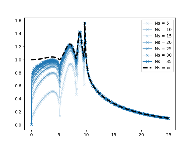
Figure 3: Spectral radius of the iteration matrix for TE-modes (and TEM-modes) on the left and TM-modes on the right with respect to $r\geq 0$ using the transmission condition (23).

Now, for a fixed frequency $k=10$, $L=1$ and overlap $\delta=0.1$, we have represented in Fig. 3 the spectral radius of $I^{\rm{TE}}(r)$ and $I^{\rm{TM}}(r)$ for various number of subdomains $N\in\{5,10,\cdots,35\}$ using the transmission conditions given by Eq. 23.

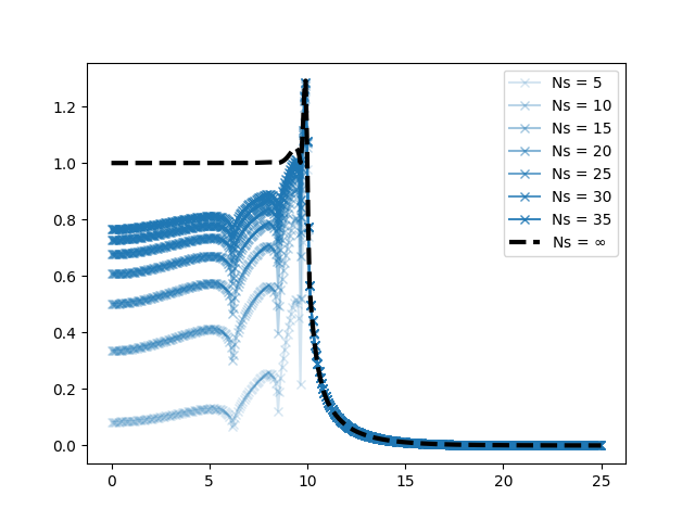
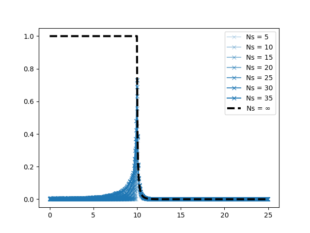
Figure 4: Spectral radius of the iteration matrix (TE or TM, it is the same) taking $\ell=0.1$ and $\sigma=5$ (on the left) and taking $\ell=1$ and $\sigma=10$ (on the right) with respect to $r\geq 0$ using the transmission condition (26).

For the same parameter, we have also represented the same quantity but using a PML transmission condition Eq. 26 with $\ell=0.1$ and $\sigma=5$, and with $\ell=1$ and $\sigma=5$ in Fig. 4.

For both transmission conditions, we can see that the convergence to the limit spectrum is fast for evanescent modes ($r\geq k$). For absorbing boundary conditions from Equation 23, the convergence to the limit spectrum is also quite fast for propagative modes. On the other hand, for PML transmission conditions from Equation 26, this convergence is bit slower for these modes and for a very strong PML (in the sense that it acts almost as the exact transmission operator). This last remark is consistent with the theory since we (almost) have $a=0$ and as we have seen, in that case all the eigenvalues of the iteration matrix tend to $0$. In this ”near nilpotency” case, the limiting spectrum result doesn’t hold any longer.

Also as expected, we can also see that PML transmission conditions lead in general to a better convergence factor than absorbing boundary conditions, and this behavirou is quite prominent for propagative modes and a lower number of subdomains.

Let us now show the impact of complex frequencies $k$, which corresponds to the case of the complex electric permittivity $\varepsilon=\varepsilon^{\prime}-\imath\varepsilon^{\prime\prime}$ with $\varepsilon^{\prime\prime}>0$. From physical point of view this means the waves are damped in an absorptive media and for this reason, the numerical computation of the solution would be easier and the underlying algorithms will converge faster. We have represented on Fig. 5 the spectral radius of the iteration matrix for TE-modes (it is the same for TM-modes as previously explained) and the limiting spectrum taking $k=10+\imath$. The results have been obtained using the same parameters as before and we tested the two transmission conditions defined in Equation 23 and Equation 26. We can see that even a (quite) small imaginary part drastically reduces the convergence factor in both cases. Also, we see that, as expected, the PML transmission conditions still lead to better results. Finally, let us mention that this time, the limit spectrum is less than one (in modulus) which shows that the iterative Schwarz algorithm will converge with a rate independent of the number of domains and hence we have weak scalability.

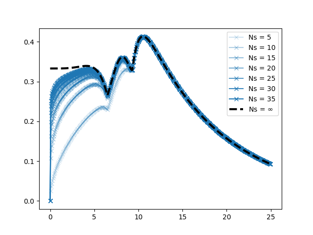
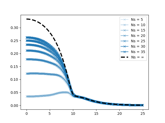
Figure 5: Spectral radius of the iteration matrix for TE-modes with respect to $r\geq 0$ using the transmission condition (23) (on the left) and (26) (on the right).

References

- [1] I. M. Babuška and S. A. Sauter, Is the pollution effect of the FEM avoidable for the Helmholtz equation considering high wave numbers?, SIAM J. Numer. Anal., 34 (1997), pp. 2392–2423.
- [2] M. Bonazzoli, V. Dolean, I. G. Graham, E. A. Spence, and P.-H. Tournier, Domain decomposition preconditioning for the high-frequency time-harmonic Maxwell equations with absorption, Math. Comp., 88 (2019), pp. 2559–2604.
- [3] N. Bootland, S. Borzooei, V. Dolean, and P.-H. Tournier, Numerical assessment of pml transmission conditions in a domain decomposition method for the helmholtz equation, in International Conference on Domain Decomposition Methods, Springer, 2022, pp. 445–453.
- [4] N. Bootland, V. Dolean, A. Kyriakis, and J. Pestana, Analysis of parallel schwarz algorithms for time-harmonic problems using block toeplitz matrices, Electronic Transactions on Numerical Analysis, 55 (2022), pp. 112–141, https://doi.org/10.1553/etna_vol55s112.
- [5] J. Bramble and J. Pasciak, Analysis of a finite pml approximation for the three dimensional time-harmonic maxwell and acoustic scattering problems, Mathematics of Computation, 76 (2007), pp. 597–614.
- [6] R. Brunet, V. Dolean, and M. J. Gander, Natural domain decomposition algorithms for the solution of time-harmonic elastic waves, SIAM J. Sci. Comput., 42 (2020), pp. A3313–A3339.
- [7] E. Cances, Y. Maday, and B. Stamm, Domain decomposition for implicit solvation models, J. Chem. Phys., 139(5) (2013), https://doi.org/10.1063/1.4816767.
- [8] G. Ciaramella and M. J. Gander, Analysis of the parallel Schwarz method for growing chains of fixed-sized subdomains: Part I, SIAM J. Numer. Anal., 55 (2017), pp. 1330–1356, https://doi.org/10.1137/16M1065215, https://doi.org/10.1137/16M1065215.
- [9] G. Ciaramella, M. Hassan, and B. Stamm, On the scalability of the Schwarz method, SMAI J. Comput. Math., 6 (2020), pp. 33–68, https://doi.org/10.5802/smai-jcm.61, https://doi.org/10.5802/smai-jcm.61.
- [10] A.-S. B.-B. Dhia and É. Lunéville, Propagation dans les guides d’ondes, (2021).
- [11] V. Dolean, M. J. Gander, and L. Gerardo-Giorda, Optimized Schwarz methods for Maxwell’s equations, SIAM J. Sci. Comput., 31 (2009), pp. 2193–2213.
- [12] V. Dolean, M. J. Gander, and A. Kyriakis, Closed form optimized transmission conditions for complex diffusion with many subdomains, SIAM Journal on Scientific Computing, 45 (2023), pp. A829–A848.
- [13] V. Dolean, M. J. Gander, S. Lanteri, J.-F. Lee, and Z. Peng, Effective transmission conditions for domain decomposition methods applied to the time-harmonic curl–curl Maxwell’s equations, J. Comput. Phys., 280 (2015), pp. 232–247, https://doi.org/10.1016/j.jcp.2014.09.024.
- [14] V. Dolean, P. Jolivet, and F. Nataf, An Introduction to Domain Decomposition Methods: Algorithms, Theory, and Parallel Implementation, SIAM, Philadelphia, 2015, https://doi.org/10.1137/1.9781611974065.ch1.
- [15] V. Dolean, P. Jolivet, P.-H. Tournier, and S. Operto, Iterative frequency-domain seismic wave solvers based on multi-level domain-decomposition preconditioners, in 82 Annual EAGE Meeting (Amsterdam), 2020. arXiv:2004.06309.
- [16] M. El Bouajaji, V. Dolean, M. J. Gander, and S. Lanteri, Optimized Schwarz methods for the time-harmonic Maxwell equations with damping, SIAM J. Sci. Comput., 34 (2012), pp. A2048–A2071.
- [17] M. J. Gander, L. Halpern, and F. Magoulès, An optimized Schwarz method with two-sided Robin transmission conditions for the Helmholtz equation, Internat. J. Numer. Methods Fluids, 55 (2007), pp. 163–175.
- [18] S. Gong, I. G. Graham, and E. A. Spence, Domain decomposition preconditioners for high-order discretizations of the heterogeneous Helmholtz equation, IMA J. Numer. Anal., (2020). draa080.
- [19] I. G. Graham, E. A. Spence, and E. Vainikko, Recent results on domain decomposition preconditioning for the high-frequency helmholtz equation using absorption, in Modern Solvers for Helmholtz Problems, D. Lahaye, J. Tang, and K. Vuik, eds., Geosystems Mathematics, Birkhäuser, Cham, 2017, pp. 3–26.
- [20] I. G. Graham, E. A. Spence, and J. Zou, Domain decomposition with local impedance conditions for the Helmholtz equation, SIAM J. Numer. Anal., 58 (2020), pp. 2515–2543.
- [21] H. Haddar, P. Joly, and H.-M. Nguyen, Generalized impedance boundary conditions for scattering problems from strongly absorbing obstacles: The case of maxwell’s equations, Mathematical Models and Methods in Applied Sciences, 18 (2008), pp. 1787–1827.
- [22] W. F. Hall and A. V. Kabakian, A sequence of absorbing boundary conditions for maxwell’s equations, Journal of Computational Physics, 194 (2004), pp. 140–155.
- [23] V. Mattesi, M. Darbas, and C. Geuzaine, A high-order absorbing boundary condition for 2D time-harmonic elastodynamic scattering problems, Comput. Math. Appl., 77 (2019), pp. 1703–1721.
- [24] A. Royer, C. Geuzaine, E. Béchet, and A. Modave, A non-overlapping domain decomposition method with perfectly matched layer transmission conditions for the helmholtz equation, Computer Methods in Applied Mechanics and Engineering, 395 (2022), p. 115006.