[a]Jeremy R. Green
Status of two-baryon scattering in lattice QCD
Abstract
In these proceedings, I will review lattice QCD calculations of baryon-baryon scattering, their methods, and their challenges. In the last few years, there has been a new generation of calculations with increased focus on controlling systematic uncertainties. Contrary to the findings of earlier exploratory calculations, it now appears probable that at heavy pion masses there is no nucleon-nucleon bound state.
1 Introduction
Lattice QCD calculations of multi-baryon systems have the ambition of deriving few-baryon interactions, which form the basis of nuclear and hypernuclear physics, starting from the Standard Model of particle physics using just a handful of experimental inputs such as the masses of the pion, kaon, and nucleon.
In addition to replacing experimental input for two- and three-baryon interactions, lattice QCD calculations can also answer questions not easily accessed. At unphysical quark masses, these calculations provide information about the dependence of the deuteron binding energy on the parameters of the Standard Model, which serves as input for studies of the fine-tunedness of the universe and whether the parameters could have been different during Big Bang nucleosynthesis [1]. Unlike in experiment, systems with strangeness are not especially challenging on the lattice, making them likely the first place lattice calculations will have an impact on phenomenology; it is hoped that precise nucleon-hyperon, hyperon-hyperon, and eventually nucleon-nucleon-hyperon interactions will help to resolve the hyperon puzzle in neutron stars [2].
Beyond scattering, lattice calculations can also include external probes, gaining insight into the structure of light nuclei. The EMC effect and quenching of axial charge revealed that interactions of a probe with more than one nucleon can contribute significantly, making it important to control these effects in particle physics experiments that use nuclear targets such as dark matter direct detection and neutrino experiments. Neutrinoless double beta decay, an inherently two-nucleon process that violates lepton number and can occur if neutrinos have a Majorana mass, is also a long-term goal [3]; it is further complicated by the need to deal with two separate currents.
Lattice QCD calculations of baryon-baryon interactions are in a state of change, transitioning from an earlier generation of exploratory calculations to new calculations with a focus on understanding and controlling systematic uncertainties, based in part on methods adapted from the last decade of successful meson-meson calculations. From these new calculations, it now appears clear that the earlier calculations were afflicted by large uncontrolled systematic uncertainties and that claims of a deeply bound deuteron and dineutron at heavy pion mass are not correct.
In this review, I will focus on calculations that use the periodic box as a tool, i.e. those based on finite-volume spectroscopy and Lüscher’s quantization condition [4, 5, 6, 7]. Alternatively, the HAL QCD method obtains hadron-hadron potentials from equal-time Nambu-Bethe-Salpeter wave functions. It has different sources of systematic uncertainty and has never claimed a deeply bound nucleon-nucleon bound state. I will say little about calculations using this method; the reader is referred to the review by Sinya Aoki at this workshop [8].
2 Methods and challenges
The standard approach for hadron-hadron interactions on the lattice proceeds by the following steps:
-
1.
Compute the low-lying finite-volume energy levels for various quantum numbers according to symmetries of the lattice theory: flavour, total momentum , and irreducible representation (irrep) of the little group containing lattice rotations and reflections that preserve . Since lattice calculations are done in cubic finite volumes of size with periodic boundary conditions, is quantized in integer multiples of . In the continuum in infinite volume, the little group irrep is given by the quantum numbers, whereas in finite volume the little group is much smaller and multiple can mix in the same irrep.
-
2.
Use finite-volume quantization conditions to constrain the scattering amplitude . Each energy level implies one constraint on the infinite set of channels and partial wave amplitudes at the corresponding centre-of-mass energy that contribute to . In practice, one must neglect partial waves beyond the lowest few and it is necessary to employ a model describing the energy-dependence of . The energy levels then serve as constraints on the parameters of the model.
-
3.
By interpolating the model along the real energy axis or extrapolating into the complex plane, find poles corresponding to bound states and resonances. Using a variety of models, one can judge the robustness of the poles and estimate systematic uncertainty from the modelling.
In addition, one must control the standard lattice systematics (which also affect the HAL QCD method): discretization effects coming from a nonzero lattice spacing , residual finite-volume effects, and unphysical quark masses . Ideally, the calculation is extrapolated , , and (or calculated directly at ). Here I will focus on the first step — computing the finite-volume spectrum — and on discretization effects, which may be more important than was expected.
2.1 Finite-volume spectroscopy
2.1.1 Excited-state effects and signal-to-noise ratio
Finite-volume spectroscopy starts with two-point correlation functions of time-local interpolating operators and with the desired quantum numbers, separated in Euclidean time. Inserting a complete set of states, we get
| (1) | ||||
where is the vacuum and are the finite-volume states of the specified quantum numbers, ordered by increasing energy. As increases, Euclidean time evolution acts as an exponential filter to remove excited states, and it is eventually possible to extract the ground-state energy from the exponential decay of . Furthermore, if then every term in the sum is positive and the effective energy will approach monotonically from above.
Complicating the matter is the well-known signal-to-noise problem [9, 10]. For a single-nucleon correlation function, the statistical error decays asymptotically with , more slowly than the correlator decays. This loss of signal makes it impossible in practice to use very large . One is reduced to looking for an acceptable “window”, where the time separation is large enough to suppress excited-state contributions but small enough that the signal is still good.
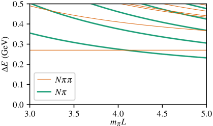
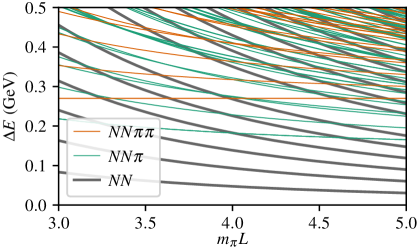
Figure 1 illustrates the approximate energy gaps between the ground state and excited states, neglecting interactions between hadrons, as functions of . In an actual calculation, the energy levels will be shifted due to those interactions as governed (in the two-particle regime) by Lüscher’s quantization condition. For a single nucleon at rest, states with the finite-volume version of quantum numbers can contribute. Here, the minimum energy gap is roughly : one can excite two pions at rest or one pion with a single unit of back-to-back momentum given to the pion and the nucleon. For a typical calculation with , these two excitations are nearly degenerate, and as , the lowest energy gap becomes .
For a two-nucleon system, the lowest energy gap is much smaller because the system can be elastically excited, i.e. each nucleon can receive one unit of momentum, yielding a gap of approximately . For the same typical calculation at the physical pion mass, this corresponds to slightly more than . Thus Euclidean time evolution is only one sixth as effective at filtering out excited states than in the single-nucleon case. In addition, the signal-to-noise ratio decays asymptotically twice as fast. The combination of these two problems is the main reason why two-nucleon systems are so challenging on the lattice: there may be no window in which the ground state has been reached but there is still a signal.
2.1.2 Improved methods
One approach to improve spectroscopy calculations is to suppress the noise. This requires modifying the standard algorithmic strategy: multilevel methods have been developed for this purpose [11, 12, 13], although they have not yet been used in a large-scale calculation. Alternatively, the filtering out of excited states can be made faster using variational methods, as is now standard in multi-meson spectroscopy. Rather than computing a single correlation function, one computes an matrix using different interpolating operators [14, 15]. By solving a generalized eigenvalue problem (GEVP)
| (2) |
for each of the lowest states one effectively finds an optimal linear combination for isolating it. The energy of state can also be estimated with a systematic error that decays asymptotically as [16]. For the ground state, this removes the contributions from the first excited states, yielding a much faster filtering by Euclidean time evolution.
2.1.3 Interpolating operators
Whether one uses a single correlator or a matrix, the starting point is interpolating operators (interpolators). Typically these are constructed using “smeared” quark fields with a spatial extent similar to the hadrons of interest. Two kinds have seen widespread use for studying two-baryon systems. The first is local “hexaquark” operators of form
| (3) |
i.e. with all six quarks at the same point. (Here, details of flavour, colour, and spin have been omitted.) These are similar to states like the dibaryon in the quark model. The second is bilocal “baryon-baryon” operators,
| (4) |
which factorize into the product of two “baryon” operators of definite momentum and thus have the structure of a noninteracting two-baryon state. Varying the single-baryon momentum allows the construction of many different operators with the same total momentum .
Given a choice of interpolating operators, computing their two-point correlation function is a nontrivial task. Since the fermionic path integral is done analytically, one must evaluate Wick contractions of quark propagators on each gauge background. Efficient solvers have been developed for the linear system , which yield applied to a specified source . Many calculations in the past have used simple smeared point sources, which imply that all smeared quarks in the creation operator lie at the same point, allowing only hexaquark interpolators. This was often paired with a baryon-baryon annihilation operator . Newer calculations use more sophisticated techniques such as distillation [17, 18] or sparsening [19], allowing a greater variety of interpolators and the use of variational methods.
2.2 Finite-volume quantization conditions
When a bound state is present, the finite-volume ground state will approach the bound-state mass with finite-volume corrections that are exponentially suppressed with , where is the binding momentum with respect to the nearest two-particle scattering threshold for particles of mass , i.e. . For shallow bound states such as the deuteron, can be small, producing slowly decaying finite-volume effects. In these cases, finite-volume quantization conditions can serve as a workaround: the finite-volume energies constrain the two-particle scattering amplitude, both above and below the bound-state mass. By interpolating, the bound-state pole can be found with much smaller finite-volume effects.
Following the initial work by Lüscher [4], two-particle finite-volume quantization conditions have been generalized to account for nonzero momentum, spin, and coupled channels [5, 6, 7]. Following Ref. [20], it can be written as , where is the reduced -matrix, related algebraically to the infinite-volume scattering amplitude; is the finite-volume matrix that depends on , , and little-group irrep; and the determinant runs over channels and partial waves. Given an ansatz for as a function of energy, its solutions are the predicted finite-volume energy levels. Truncated to a single channel and partial wave, it becomes a simple equation giving the phase shift at the centre-of-mass energy corresponding to each finite-volume energy level.
It has been known for a long time that finite-volume quantization conditions break down above the lowest untreated threshold, which typically corresponds to three particles. However, it was noted in Ref. [21] that a breakdown also occurs somewhere below the lowest two-particle threshold, due to left-hand cuts. This is particularly relevant for baryon-baryon systems, in which pion exchange causes left-hand cuts to occur close to the lowest threshold. With several new proposals on how to deal with this issue [22, 23, 24, 25, 26, 27, 28], this is an ongoing area of research and the reader is referred to the talks on this subject presented at this workshop [29, 30, 31, 32, 33]. Another direction being investigated is how to include lattice artifacts that break symmetry [34].
3 Old and new calculations
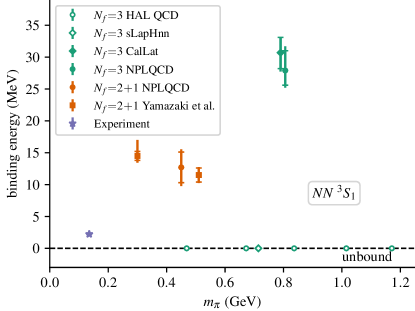
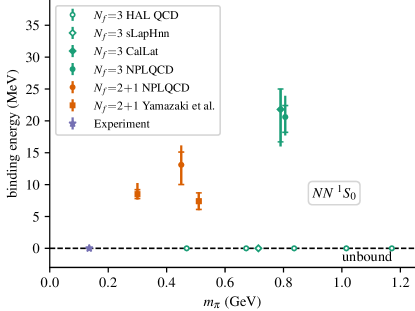
There has been a decade-long controversy over whether nucleon-nucleon bound states exist for QCD with heavier-than-physical quark masses; see Fig. 2. Some calculations reported that the deuteron becomes more deeply bound as the pion mass is increased, and that a second “dineutron” (isospin one, spin zero) bound state appears [41, 40, 37, 42, 43, 44, 38, 39]. However, first HAL QCD and then others reported the opposite result: that there is no bound state [35, 36]. More recent calculations for which preliminary results were reported [45] or where conclusions about the presence of bound states were not reached [46, 47] are also consistent with there being no bound state.
The presence or absence of nucleon-nucleon bound states is one of the simplest questions about nuclear physics that can be asked of lattice QCD. This long-standing disagreement is a significant problem that needs to be resolved before lattice calculations of other two-baryon observables can be taken seriously. Fortunately, a new generation of calculations promises to better control systematic uncertainties and resolve the controversy.
What explains the disagreement in Fig. 2? One possible source is discretization effects: except for recent calculations in Refs. [21, 48, 45, 49, 50], no baryon-baryon study used more than one lattice spacing . Thus, the missing extrapolation is a completely uncontrolled source of systematic error. Another source is excited states contaminating the estimate of the ground-state energy. Calculations that obtained bound states used point-source methods and asymmetric correlation functions of form , whereas calculations yielding no bound state used either the HAL QCD method (with very different systematics) or variational methods [36, 45, 46, 47].
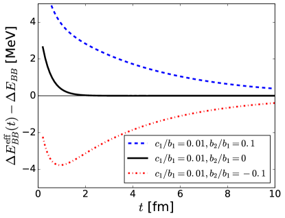
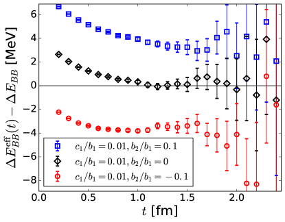
The question of how a spectroscopy calculation can go wrong has been studied by HAL QCD [51]. If variational methods are not used, then the very small energy gap between the ground state and lowest-lying elastic excitation controls the asymptotic approach to the energy plateau. The need for implies that Euclidean time separations of up to 10 fm are needed to isolate the ground-state energy. Furthermore, an asymmetric correlation function allows excited-state contributions of either sign, further confounding the plateau. Given that the noise starts to grow rapidly for fm, this can cause “fake plateaus” to appear; see Fig. 3. In particular, noise transforms the case with a local minimum into the best-looking plateau.
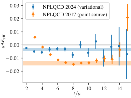
This effect can be seen in two sets of calculations done by NPLQCD on the same lattice ensembles at a heavy SU(3)-symmetric point ( MeV). The earlier work [43, 38], which used point sources and asymmetric correlators, found a dineutron ( ) bound state with binding energy MeV. The newer work [46, 47], which used variational techniques with a variety of local and bilocal interpolating operators, is consistent with no bound state. As shown in Fig. 4, the two calculations produced quite incompatible energy plateaus. Since variational methods yield better control over low-lying excited states, the newer calculation has a more trustworthy plateau. For further discussion on this issue, see Refs. [52, 53].
4 Calculations at light SU(3)-symmetric point
In this section I will report some past and ongoing calculations that I have done together with the “Mainz group” and the broader Baryon Scattering (BaSc) collaboration. These have been done using ensembles from CLS [57] at an SU(3)-symmetric point where the up, down, and strange quarks are degenerate with mass set to the average of their masses in nature, corresponding to MeV. We employed variational methods to study multiple low-lying energy levels and eight lattice ensembles covering a range of different box sizes and lattice spacings .
4.1 Nucleon-nucleon and
Flavour symmetries are unbroken on the lattice and the two-particle quantization condition does not mix different spins, allowing us to analyze four different subsets of nucleon-nucleon energy levels independently: combining spin zero or one with isospin zero or one. The simplest of these to analyze is isospin-zero spin-zero, which contains odd partial waves , , , etc. The corresponding energy levels are shown in Fig. 5. In all cases, the lattice energy is shifted upward relative to the noninteracting one, indicating a repulsive interaction.
The lattice spectrum can be fitted using a chiral EFT-inspired model for the and phase shifts combined with finite-volume quantization. I include the one-pion-exchange potential and one contact term in each partial wave, regularized following Ref. [59] with cutoff , and solve the Lippmann-Schwinger equation to obtain the phase shifts. With just three fit parameters ( and the coefficients of the two contact terms) and assuming no discretization effects, this model provides a good description of the spectrum and a reasonable-valued coupling constant . However, in a sign of the breakdown of the quantization condition, there are also spurious solutions that converge toward the onset of the left-hand cut as . Here they can be easily skipped over, since the spectra start well above threshold; however, spurious solutions are potentially problematic for analyzing waves, which are constrained by near-threshold energy levels.
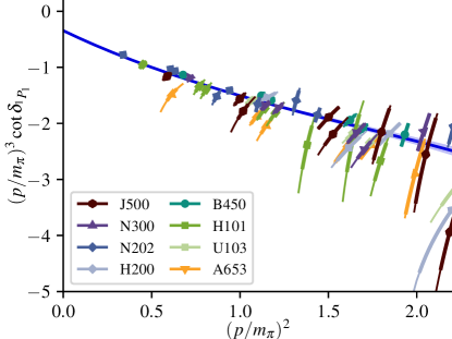
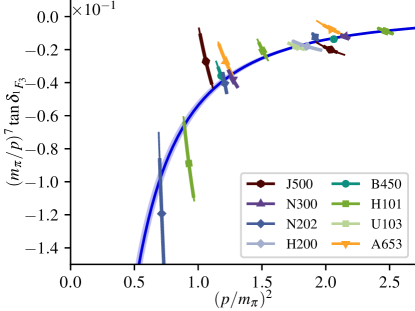
The corresponding phase shifts are shown in Fig. 6. In a highly nontrivial check of the finite-volume spectrum, all of the phase-shift points from different volumes, moving frames, and irreps lie on a single curve, suggesting that the uncertainties of the spectrum are under reasonable control. Furthermore, the different lattice spacings agree, indicating that discretization effects are small.
4.2 dibaryon
Conjectured decades ago based on an MIT bag model calculation [60], the dibaryon is a hypothetical SU(3) flavour singlet scalar that would be a bound state. Past lattice calculations [61, 35, 62, 63, 64, 42, 43] have also found bound states for heavy quark masses, with binding energies of up to 75 MeV. This includes calculations by HAL QCD, who have consistently found no nucleon-nucleon bound state. However, at similar quark masses corresponding to MeV, the binding energy reported by HAL QCD is about half as big as the one reported by NPLQCD.
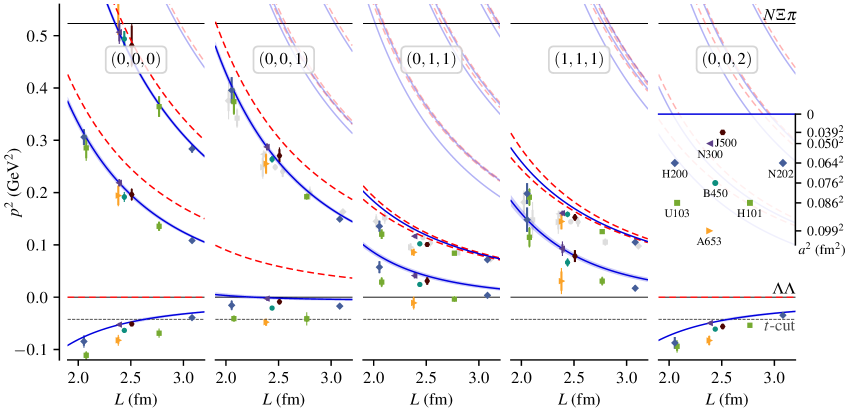
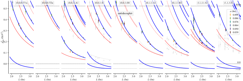
Our finite-volume spectra relevant for the dibaryon at the light SU(3)-symmetric point are shown in Fig. 7. There are two notable features. First, there is a strong dependence on the lattice spacing: the difference between noninteracting and lattice energies can vary by a factor of almost two between the finest and coarsest lattices. This was a surprising result, as it had been expected that discretization effects would mostly cancel in this difference. Second, the lowest energy levels lie on top of the left-hand cut, making them unusable in Lüscher’s finite-volume quantization condition.
In Ref. [21], we fitted these data by describing with polynomials in , allowing the coefficients to depend on the lattice spacing. The levels on the left-hand cut were omitted from the analysis. In the continuum limit, we found a binding energy of roughly 5 MeV, whereas at nonzero lattice spacing this was up to seven times larger. This difference is comparable in size to the spread between past studies of the dibaryon, which each used just a single lattice spacing.
For two-nucleon energy levels, preliminary results in irreps that contain and – partial waves also show significant dependence on the lattice spacing [48, 45], in contrast with the spin-zero odd partial waves shown in the previous subsection. Recently, significant lattice artifacts for the dibaryon binding energy have also been found by HAL QCD [49] (with otherwise very different systematics) and NPLQCD [50]. Thus, the need for fine lattice spacings and good control over the continuum limit adds to the challenges in studying two-baryon systems on the lattice.
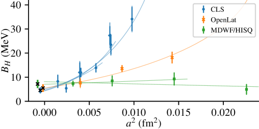
Together with the broader BaSc collaboration, I have been studying the origin of these discretization effects by repeating the study of the dibaryon using different lattice formulations of QCD [65, 66]. We supplemented the existing calculation on CLS ensembles using clover fermions from Ref. [21] with two other actions with the same quark masses. First, we used three ensembles with a modified clover term [67] from OpenLat [68]. Second, we generated four staggered-fermion ensembles with the HISQ action [69, 70] (including a physical-mass charm quark) and used Möbius domain wall valence fermions in a mixed-action setup [71]. As shown in Fig. 8, these other actions produce a much weaker dependence on the lattice spacing, which might help future calculations control discretization effects at a lower computational cost.
5 Summary and outlook
Following increased scrutiny, it now appears probable that past exploratory lattice QCD calculations of two-baryon systems were affected by two sources of large uncontrolled systematic uncertainty: the ground-state energy was not adequately isolated and discretization effects were neglected. In particular, there is no nucleon-nucleon bound state at significantly-heavier-than-physical pion masses.
Moving forward, the community needs to maintain its focus on controlling systematic effects. A better understanding of lattice artifacts, their origin, and how to model them, would be quite valuable. Applying modified quantization conditions that account for the left-hand cut will help to control and understand the residual finite-volume effects. In general, it will be important to have more detailed cross-checks between different collaborations including HAL QCD (with its different methodology): rather than simply agreeing on the absence of a bound state, we should quantitatively compare scattering lengths, effective ranges, phase shifts, and mixing angles.
Finally, we need to push to lighter quark masses, towards the physical point. As the signal-to-noise problem becomes more severe and the energy splittings become smaller, new techniques may be needed to make the calculations feasible.
Acknowledgments
I thank my colleagues in the BaSc collaboration for valuable discussions. Calculations for these projects used resources provided by the John von Neumann Institute for Computing and Gauss Centre for Supercomputing e.V. (www.gauss-centre.eu) on JUQUEEN [72], JURECA [73], and JUWELS [74] at Jülich Supercomputing Centre; on Summit at the Oak Ridge Leadership Computing Facility at the Oak Ridge National Laboratory, which is supported by the Office of Science of the U.S. Department of Energy under Contract No. DE-AC05-00OR22725; provided by the Lawrence Livermore National Laboratory (LLNL) Multiprogrammatic and Institutional Computing program for Grand Challenge allocations on Lassen at LLNL; and of the National Energy Research Scientific Computing Center (NERSC), a Department of Energy Office of Science User Facility using NERSC awards NP-ERCAP0033436 and NP-ERCAP0027666. This work used the software packages GLU [75], QDP++ [76], PRIMME [77], openQCD [78], QUDA [79, 80, 81], opt_einsum [82], SigMonD [83], TwoHadronsInBox [20], NumPy [84], SciPy [85], and Matplotlib [86]. We are grateful to our colleagues within CLS and OpenLat for sharing ensembles.
References
- [1] H. Meyer, U.-G. Meißner and B. Metsch, Anthropic considerations for Big Bang nucleosynthesis, PoS CD2024 113.
- [2] A. Nogga, Application of chiral two- and three-baryon interactions to light hypernuclei, PoS CD2024 090.
- [3] J. de Vries, Neutrinoless double beta decay and chiral effective field theory, PoS CD2024 022.
- [4] M. Lüscher, Nucl. Phys. B 354 (1991) 531.
- [5] K. Rummukainen and S.A. Gottlieb, Nucl. Phys. B 450 (1995) 397 [hep-lat/9503028].
- [6] R.A. Briceño, Z. Davoudi and T.C. Luu, Phys. Rev. D 88 (2013) 034502 [1305.4903].
- [7] R.A. Briceño, Phys. Rev. D 89 (2014) 074507 [1401.3312].
- [8] S. Aoki, Interactions between two hadrons in lattice QCD, PoS CD2024 018.
- [9] G. Parisi, Phys. Rept. 103 (1984) 203.
- [10] G.P. Lepage, The analysis of algorithms for lattice field theory, in From Actions to Answers: Proceedings of the 1989 Theoretical Advanced Study Institute in Elementary Particle Physics, T. DeGrand and D. Toussaint, eds., pp. 97–120, World Scientific, 1989.
- [11] M. Cè, L. Giusti and S. Schaefer, Phys. Rev. D 93 (2016) 094507 [1601.04587].
- [12] M. Cè, L. Giusti and S. Schaefer, Phys. Rev. D 95 (2017) 034503 [1609.02419].
- [13] L. Giusti and M. Saccardi, Phys. Lett. B 829 (2022) 137103 [2203.02247].
- [14] C. Michael, Nucl. Phys. B 259 (1985) 58.
- [15] M. Lüscher and U. Wolff, Nucl. Phys. B 339 (1990) 222.
- [16] B. Blossier, M. Della Morte, G. von Hippel et al., JHEP 04 (2009) 094 [0902.1265].
- [17] Hadron Spectrum collaboration, Phys. Rev. D 80 (2009) 054506 [0905.2160].
- [18] C. Morningstar, J. Bulava, J. Foley et al., Phys. Rev. D 83 (2011) 114505 [1104.3870].
- [19] W. Detmold et al., Phys. Rev. D 104 (2021) 034502 [1908.07050].
- [20] C. Morningstar, J. Bulava, B. Singha et al., Nucl. Phys. B 924 (2017) 477 [1707.05817].
- [21] J.R. Green, A.D. Hanlon, P.M. Junnarkar and H. Wittig, Phys. Rev. Lett. 127 (2021) 242003 [2103.01054].
- [22] L. Meng and E. Epelbaum, JHEP 10 (2021) 051 [2108.02709].
- [23] L. Meng, V. Baru, E. Epelbaum et al., Phys. Rev. D 109 (2024) L071506 [2312.01930].
- [24] A.B. Raposo and M.T. Hansen, JHEP 08 (2024) 075 [2311.18793].
- [25] M.T. Hansen, F. Romero-López and S.R. Sharpe, JHEP 06 (2024) 051 [2401.06609].
- [26] S.M. Dawid, F. Romero-López and S.R. Sharpe, JHEP 01 (2025) 060 [2409.17059].
- [27] R. Bubna, H.-W. Hammer, F. Müller et al., JHEP 05 (2024) 168 [2402.12985].
- [28] S.M. Dawid, A.W. Jackura and A.P. Szczepaniak, 2411.15730.
- [29] M.T. Hansen, Left-hand branch cuts in lattice QCD scattering calculations, PoS CD2024 006.
- [30] A. Rusetsky, R. Bubna, H.W. Hammer et al., Long-range forces in a finite volume, PoS CD2024 045.
- [31] L. Meng, Left-hand cut problem in lattice QCD and an EFT-based solution, PoS CD2024 046.
- [32] S. Dawid, Three-body analysis of , PoS CD2024 048.
- [33] F. Romero-López, Three-hadron dynamics from lattice QCD, PoS CD2024 007.
- [34] M.T. Hansen and T. Peterken, 2408.07062.
- [35] HAL QCD collaboration, Nucl. Phys. A 881 (2012) 28 [1112.5926].
- [36] B. Hörz et al., Phys. Rev. C 103 (2021) 014003 [2009.11825].
- [37] E. Berkowitz, T. Kurth, A. Nicholson et al., Phys. Lett. B 765 (2017) 285 [1508.00886].
- [38] M.L. Wagman, F. Winter, E. Chang et al., Phys. Rev. D 96 (2017) 114510 [1706.06550].
- [39] NPLQCD collaboration, Phys. Rev. D 103 (2021) 054508 [2009.12357].
- [40] T. Yamazaki et al., Phys. Rev. D 86 (2012) 074514 [1207.4277].
- [41] T. Yamazaki et al., Phys. Rev. D 92 (2015) 014501 [1502.04182].
- [42] NPLQCD collaboration, Phys. Rev. D 85 (2012) 054511 [1109.2889].
- [43] NPLQCD collaboration, Phys. Rev. D 87 (2013) 034506 [1206.5219].
- [44] NPLQCD collaboration, Phys. Rev. D 92 (2015) 114512 [1508.07583], [Erratum: Phys. Rev. D 102 (2020) 039903].
- [45] Baryon Scattering (BaSc) collaboration, PoS LATTICE2022 (2023) 200 [2212.09587].
- [46] S. Amarasinghe, R. Baghdadi, Z. Davoudi et al., Phys. Rev. D 107 (2023) 094508 [2108.10835], [Erratum: Phys. Rev. D 110 (2024) 119904].
- [47] W. Detmold, M. Illa, W.I. Jay et al., 2404.12039.
- [48] J.R. Green, A.D. Hanlon, P.M. Junnarkar and H. Wittig, PoS LATTICE2021 (2022) 294 [2111.09675].
- [49] HAL QCD collaboration, Few Body Syst. 65 (2024) 34.
- [50] R. Perry et al., Studying lattice artifacts in baryon-baryon variational bounds, PoS LATTICE2024 125.
- [51] T. Iritani et al., JHEP 10 (2016) 101 [1607.06371].
- [52] HAL QCD collaboration, JHEP 03 (2019) 007 [1812.08539].
- [53] R. Briceño, J.R. Green, A.D. Hanlon, A. Nicholson and A. Walker-Loud, On the reliable lattice-QCD determination of multi-baryon interactions and matrix elements, in Nuclear Forces for Precision Nuclear Physics: A Collection of Perspectives, I. Tews, Z. Davoudi, A. Ekström and J.D. Holt, eds., Few Body Syst. 63 (2022) 67 [2202.01105].
- [54] A. Francis, J.R. Green, P.M. Junnarkar, C. Miao, T.D. Rae and H. Wittig, Phys. Rev. D 99 (2019) 074505 [1805.03966].
- [55] Y. Geng, L. Liu, P. Sun et al., Doubly charmed -like dibaryon scattering from lattice QCD, PoS LATTICE2024 307.
- [56] Z.-Y. Wang, X. Feng, L. Jin and C. Liu, Lattice calculation of proton-proton fusion matrix element, PoS LATTICE2024 111.
- [57] M. Bruno et al., JHEP 02 (2015) 043 [1411.3982].
- [58] Baryon Scattering (BaSc) collaboration, Two nucleons from SU(3)-flavor-symmetric QCD, in preparation.
- [59] P. Reinert, H. Krebs and E. Epelbaum, Eur. Phys. J. A 54 (2018) 86 [1711.08821].
- [60] R.L. Jaffe, Phys. Rev. Lett. 38 (1977) 195 [Erratum: Phys. Rev. Lett. 38 (1977) 617].
- [61] HAL QCD collaboration, Phys. Rev. Lett. 106 (2011) 162002 [1012.5928].
- [62] HAL QCD collaboration, Nucl. Phys. A 998 (2020) 121737 [1912.08630].
- [63] NPLQCD collaboration, Phys. Rev. Lett. 106 (2011) 162001 [1012.3812].
- [64] S.R. Beane et al., Mod. Phys. Lett. A 26 (2011) 2587 [1103.2821].
- [65] J.R. Green et al., Universality of the continuum limit for the dibaryon, talk presented at Lattice 2024.
- [66] Baryon Scattering (BaSc) collaboration, Universality of the continuum limit for the dibaryon, in preparation.
- [67] A. Francis et al., Comput. Phys. Commun. 255 (2020) 107355 [1911.04533].
- [68] A. Francis, F. Cuteri, P. Fritzsch et al., PoS LATTICE2023 (2024) 048 [2312.11298].
- [69] HPQCD, UKQCD collaboration, Phys. Rev. D 75 (2007) 054502 [hep-lat/0610092].
- [70] MILC collaboration, Phys. Rev. D 82 (2010) 074501 [1004.0342].
- [71] E. Berkowitz et al., Phys. Rev. D 96 (2017) 054513 [1701.07559].
- [72] Jülich Supercomputing Centre, J. Large-Scale Res. Facil. 1 (2015) A1.
- [73] Jülich Supercomputing Centre, J. Large-Scale Res. Facil. 4 (2018) A132.
- [74] Jülich Supercomputing Centre, J. Large-Scale Res. Facil. 7 (2021) A183.
- [75] R.J. Hudspith, “GLU.” https://github.com/RJHudspith/GLU, Feb., 2014.
- [76] SciDAC, LHPC, UKQCD collaboration, Nucl. Phys. B (Proc. Suppl.) 140 (2005) 832 [hep-lat/0409003].
- [77] A. Stathopoulos and J.R. McCombs, ACM Trans. Math. Softw. 37 (2010) 21:1.
- [78] M. Lüscher and S. Schaefer, “openQCD.” http://luscher.web.cern.ch/luscher/openQCD/, 2012.
- [79] QUDA collaboration, Comput. Phys. Commun. 181 (2010) 1517 [0911.3191].
- [80] QUDA collaboration, Scaling lattice QCD beyond 100 GPUs, in SC ’11: Proceedings of the International Conference for High Performance Computing, Networking, Storage and Analysis, 9, 2011 [1109.2935].
- [81] QUDA collaboration, Accelerating lattice QCD multigrid on GPUs using fine-grained parallelization, in SC ’16: Proceedings of the International Conference for High Performance Computing, Networking, Storage and Analysis, 12, 2016 [1612.07873].
- [82] D.G.A. Smith and J. Gray, J. Open Source Softw. 3(26) (2018) 753.
- [83] C. Morningstar, “SigMonD.” https://github.com/andrewhanlon/sigmond, Feb., 2023.
- [84] C.R. Harris, K.J. Millman, S.J. van der Walt et al., Nature 585 (2020) 357 [2006.10256].
- [85] P. Virtanen, R. Gommers, T.E. Oliphant et al., Nature Methods 17 (2020) 261 [1907.10121].
- [86] J.D. Hunter, Comput. Sci. Eng. 9 (2007) 90.