Generalization Guarantees for Representation Learning via Data-Dependent Gaussian Mixture Priors

Abstract

We establish in-expectation and tail bounds on the generalization error of representation learning type algorithms. The bounds are in terms of the relative entropy between the distribution of the representations extracted from the training and “test” datasets and a data-dependent symmetric prior, i.e., the Minimum Description Length (MDL) of the latent variables for the training and test datasets. Our bounds are shown to reflect the “structure” and “simplicity” of the encoder and significantly improve upon the few existing ones for the studied model. We then use our in-expectation bound to devise a suitable data-dependent regularizer; and we investigate thoroughly the important question of the selection of the prior. We propose a systematic approach to simultaneously learning a data-dependent Gaussian mixture prior and using it as a regularizer. Interestingly, we show that a weighted attention mechanism emerges naturally in this procedure. Our experiments show that our approach outperforms the now popular Variational Information Bottleneck (VIB) method as well as the recent Category-Dependent VIB (CDVIB).

1 Introduction

One major problem in learning theory pertains to how to guarantee that a statistical learning algorithm performs on new, unseen data as well as on the used training data, i.e., it has good generalization properties. This key question, which has roots in various scientific disciplines, has been studied using seemingly unrelated approaches, including compression-based [59; 14; 7; 13; 83; 47; 9; 39; 41; 15; 40; 42; 20; 78; 77], information-theoretic [75; 89; 82; 30; 17; 37; 66; 5; 43; 91; 61; 44], PAC-Bayes [76; 57; 18; 63; 34; 86; 10; 84; 28; 67; 72; 64; 65; 88], and intrinsic dimension-based [81; 12; 46; 58] approaches.

In practice, a common approach advocates the usage of a two-part, or encoder-decoder, model, often referred to as representation learning. In this approach, the encoder part of the model shoots for extracting a “minimal” representation of the input (i.e., small generalization error), whereas the decoder part shoots for small empirical risk. One popular approach is the information bottleneck (IB), which was first introduced in  [85] and then extended in various ways [80; 3; 2; 55; 31; 73; 53]. The IB principle is mainly based on the assumption that Shannon’s mutual information (MI) between the input and the representation is a good indicator of the generalization error. However, this assumed relationship has been refuted in several works [54; 74; 6; 32; 23; 62; 79]. As shown in these works, the few existing theoretical MI-based generalization bounds (e.g., [87; 49]) become vacuous in most reasonable setups. Also, in practice, no consistent relation between the generalization error and the MI has been observed experimentally so far. Rather, recent works [13; 32; 79] have shown that the generalization error of representation learning algorithms is related to the minimum description length (MDL) of the latent variable and the so-called geometric compression. Geometric compression occurs when latent vectors are designed so as to concentrate around a limited number of representatives which form centroid vectors of associated clusters [6; 32]. In such settings, inputs can be mapped to the centroids of the clusters that are closest to their associated latent vectors (i.e., lossy compression); and this yields non-vacuous bounds at the expense of only a small (distortion) penalty. The benefit of this lossy compression approach can be appreciated when opposed to classic MI-based bounds [87; 49] which are known to be vacuous when the latent vectors are deterministic functions of the inputs.

In this work, we study the problem of representation learning depicted in Fig. 1 from a generalization error perspective. Then, we use the obtained generalization bound to design and discuss various choices of generalization-inspired regularizers using data-dependent Gaussian mixture priors. To the best knowledge of the authors, generalization error bounds that account suitably for the encoder-decoder structure of the representation learning problem of Fig. 1 are very scarce; and, in fact, with the exception of [79], no non-vacuous bounds for this settings have been reported so far.

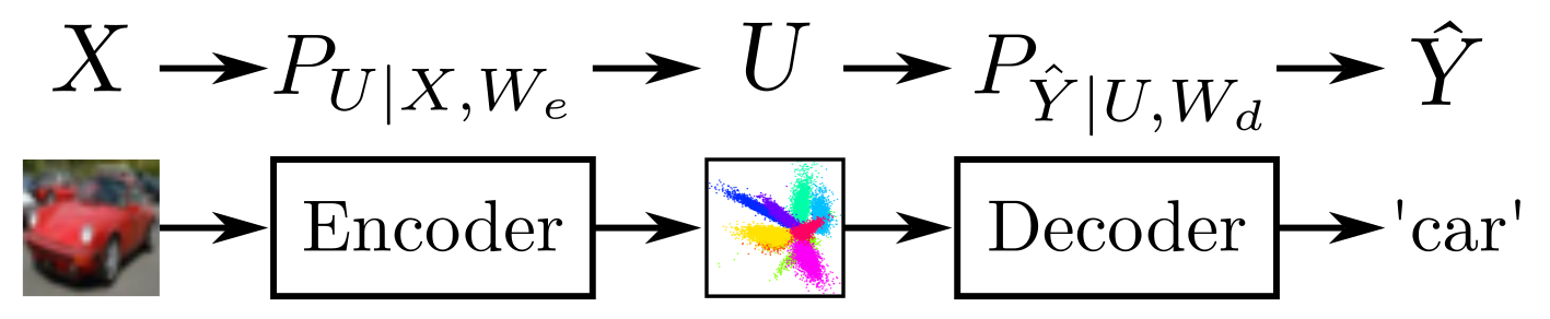
Figure 1: Studied representation learning setup.

Contributions: Our main contributions in this work are summarized as follows.

• We establish in-expectation and tail bounds on the generalization error of the representation learning algorithms. Our bounds are expressed in terms of the relative entropy between the distribution of the representations extracted from training and “test” datasets and a data-dependent symmetric prior $\mathbf{Q}$, i.e., the Minimum Description Length ($\text{MDL}(\mathbf{Q})$) of the latent variables for training and test datasets – (Bounds that depend on $\text{MDL}(\mathbf{Q})$ are arguably better bounds because they capture the structure and simplicity of the encoders in sharp contrast with IB-based approaches [13]). However, our bounds are shown to be possibly tighter than those of [79]. For instance, while the bounds of [79] are of the order of $\sqrt{\text{MDL}(\mathbf{Q})/n}$, where $n$ designates the size of the used training dataset, ours is approximately of the order of $\text{MDL}(\mathbf{Q})/n$ for the realizable setup.

• We propose a systematic approach to finding a suitable “data-dependent” prior that we then use to construct judiciously a regularizer during training (based on our newly established bounds). Specifically, first, we observe that if the latent variables are generated according to a Gaussian distribution, then the prior $\mathbf{Q}$ that minimizes the empirical $\text{MDL}(\mathbf{Q})$ term is a Gaussian mixture distribution. Then, using this and the known fact that Gaussian mixture distributions can approximate sufficiently well any arbitrary distribution when the number of mixture components is large enough [21; 36; 69], we propose two methods for simultaneously finding a Gaussian mixture prior and using it as a regularizer along the optimization iterations. The methods are coined ‘lossless Gaussian mixture prior” and “lossy Gaussian mixture prior”, respectively. In essence, the procedure consists of finding the underlying “structure” of the latent variables in the form of a Gaussian mixture prior; and, simultaneously, steers the latent variables to best fit with this found structure. Interestingly, in the lossy version of the approach, which is shown to generally yield better performance, the components of the Gaussian mixture are updated using a mechanism that is similar to the self-attention mechanism. In particular, the components are updated according to the extent they each “attend” to the latent variables statistically.

• We validate the advantages of our generalization-aware regularizer in practice through experiments using various datasets (CIFAR10, CIFAR100, INTEL, and USPS) and encoder architectures (CNN4 and ResNet18). In particular, we show that our approach outperforms the popular VIB of [3] and the recent Category-Dependent VIB of [79]. The reader is referred to Section 5 and Appendix E for details on the datasets, models, and experiments.

We emphasize once more that our approach here, which measures complexity using MDL of the involved latent variables, has two appealing features: (i) it yields generalization bounds that only depend on the encoder part of representation type statistical learning algorithms, and (ii) the employed lossy compression enables the yielded bounds to only take finite values, i.e., not vacuous, in reasonable setups, by opposition to the MI bounds of [87; 49]. The described approach and results must be contrasted with classes of prior-art bounds that measure complexity differently. The first class of bounds involves the complexity of the hypothesis (model) space and includes, e.g., MI-based, PAC-Bayes, and some of the compression-based bounds (e.g. [7]). Such bounds mostly involve “data-independent” priors on the model; and seldom use “data-dependent” priors [29; 71] – see [4, Section 3.3] for a detailed review. Generalization bounds that use model complexity do not seem to be amenable to using them for regularization since, in practice, one has only a single instance of the posterior. The second class of bounds are intrinsic dimension-based bounds that measure the complexity of the model along the optimization trajectories. Although in this approach multiple instances of the posterior are available, measuring the trajectory complexity of large models is not practical. The third class of bounds uses prediction complexity such as with f-CMI [43; 44] - see also the related [13; 79]. In such bounds, typically the complexity appears in both the loss function and the regularizer; and this is generally not reasonable in practice.

Notations. We denote the random variables and their realizations by upper and lower case letters and use Calligraphy fonts to refer to their support set e.g., $X$, $x$, and $\mathcal{X}$. The distribution of $X$ is denoted by $P_{X}$, which for simplicity, is assumed to be a probability mass function for a random variable with discrete support set and to be probability density function otherwise. With this assumption, the Kullback–Leibler (KL) between two distributions $P$ and $Q$ is defined as $D_{KL}\left(P\|Q\right)\coloneqq\mathbb{E}_{P}\left[\log(P/Q)\right]$ if $P\ll Q$, and $\infty$ otherwise. Lastly, we denote the set $\{1,\ldots,n\}$, $n\in\mathbb{N}^{*}$, by $[n]$.

2 Problem setup

We consider a $C$-class classification setup, as described below.

Data. We assume that the input data $Z$, which take value according to an unknown distribution $\mu$, is composed of two parts $Z=(X,Y)$, where (i) $X$ represents the feature of the input data, taking values in the feature space $\mathcal{X}$, and (ii) $Y\in\mathcal{Y}$ represents the label ranging from 1 to $C$, i.e., $\mathcal{Y}=[C]$. We denote the underlying distribution of $X$ and $Y$ by $\mu_{X}$ and $\mu_{Y}$, respectively, and their joint distribution by $\mu\coloneqq\mu_{X|Y}\mu_{Y}\coloneqq\mu_{X}\mu_{Y|X}$.

Training dataset. To learn a model, we assume the availability of a training dataset $S=\{Z_{1},\ldots,Z_{n}\}\sim\mu^{\otimes n}\eqqcolon P_{S}$, composed of $n$ i.i.d. samples $Z_{i}=(X_{i},Y_{i})$ of the input data. In our analysis, we often use a test dataset (known also as ghost dataset [82]) $S^{\prime}=\{Z^{\prime}_{1},\ldots,Z^{\prime}_{n}\}\sim\mu^{\otimes n}\eqqcolon P_{S^{\prime}}$, where $Z^{\prime}_{i}=(X^{\prime}_{i},Y^{\prime}_{i})$. To simplify the notation, we denote the features and labels of $S$ and $S^{\prime}$ by $\mathbf{X}\coloneqq X^{n}\sim\mu_{X}^{\otimes n}$, $\mathbf{Y}\coloneqq Y^{n}\sim\mu_{Y}^{\otimes n}$, $\mathbf{X}^{\prime}\coloneqq X^{\prime n}\sim\mu_{X}^{\otimes n}$, and $\mathbf{Y}^{\prime}\coloneqq Y^{\prime n}\sim\mu_{Y}^{\otimes n}$, respectively.

Encoder-decoder model. We assume that the model (hypothesis) is composed of two parts: an encoder and a decoder part. The encoder $w_{e}\in\mathcal{W}_{e}$ takes as input the feature $x$ and generates as output the representation or the latent variable $U\in\mathcal{U}$, possibly stochastically. For simplicity, we assume that $\mathcal{U}=\mathbb{R}^{d}$, for some $d\in\mathbb{N}^{*}$. The decoder $w_{d}\in\mathcal{W}_{d}$ takes $U$ as input and outputs an estimate $\hat{Y}$ of the true label $Y$. The overall model is denoted by $w\coloneqq(w_{e},w_{d})\in\mathcal{W}=\mathcal{W}_{e}\times\mathcal{W}_{d}$. The setup is shown in Fig. 1.

Learning algorithm. We consider a general stochastic learning framework in which the learning algorithm $\mathcal{A}\colon\mathcal{Z}^{n}\to\mathcal{W}$ has access to a training dataset $S$ and uses it to choose a model (or hypothesis) $\mathcal{A}(S)=W\in\mathcal{W}$, where $W=(W_{e},W_{d})$. The distribution induced by the learning algorithm $\mathcal{A}$ is denoted by $P_{W|S}=P_{W_{e},W_{d}|S}$. Also, the joint distribution of $(S,W)$ is denoted by $P_{S,W}$ and the marginal distribution of $W$ under this distribution is denoted by $P_{W}$. Furthermore, we denote the induced conditional distribution of the latent variable $U$ given the encoder and the input by $P_{U|X,W_{e}}$. Finally, we denote the conditional distribution of the model’s prediction $\hat{Y}$, conditioned on the decoder and the latent variable, by $P_{\hat{Y}|U,W_{d}}$. It is easy to see that $P_{\hat{Y}|X,W}=\mathbb{E}_{U\sim P_{U|X,W_{e}}}\big{[}P_{\hat{Y}|U,W_{d}}\big{]}$. Lastly and as a general rule, we use the following shorthand notation

$$P_{\mathbf{U},\mathbf{U}^{\prime}|\mathbf{X},\mathbf{X}^{\prime},W_{e}}\coloneq\bigotimes\nolimits_{i\in[n]}\left\{P_{U_{i}|X_{i},W_{e}}P_{U^{\prime}_{i}|X^{\prime}_{i},W_{e}}\right\}.$$ (1)

Similar notation is used to shorten products of distributions, e.g., $P_{\mathbf{U}|\mathbf{X},W_{e}}$ and $P_{\hat{\mathbf{Y}}|\mathbf{X},W}$.

Risks. The quality of a model $w$ is assessed by the below 0-1 loss function $\ell\colon\mathcal{Z}\times\mathcal{W}\to\{0,1\}$:

$$\ell(z,w)\coloneqq\mathbb{E}_{\hat{Y}\sim P_{\hat{Y}|x,w}}[\mathbbm{1}_{\{y\neq\hat{Y}\}}]=\mathbb{E}_{U\sim P_{U|x,w_{e}}}\mathbb{E}_{\hat{Y}\sim P_{\hat{Y}|U,w_{d}}}\left[\mathbbm{1}_{\{y\neq\hat{Y}\}}\right].$$ (2)

In learning theory, the ultimate goal is to find a model that minimizes the population risk, defined as $\mathcal{L}(w)\coloneqq\mathbb{E}_{Z\sim\mu}\left[\ell(Z,w)\right]$. However, since the underlying distribution $\mu$ is unknown, only the empirical risk, defined as $\hat{\mathcal{L}}(s,w)\coloneqq\frac{1}{n}\sum_{i\in[n]}\ell(z_{i},w)$, is accessible and can be minimized. Therefore, a central question in learning theory and this paper is to control the difference between these two risks, known as generalization error:

$$\operatorname{gen}(s,w)\coloneqq\mathcal{L}(w)-\hat{\mathcal{L}}(s,w).$$ (3)

In our results, for simplicity, we also use the following shorthand notations:

$$\mathcal{\hat{L}}(\mathbf{y},\mathbf{\hat{y}})\coloneqq\frac{1}{n}\sum\nolimits_{i\in[n]}\mathbbm{1}_{\{\hat{y}_{i}\neq y_{i}\}}, \quad\quad\mathcal{\hat{L}}(\mathbf{y}^{\prime},\mathbf{\hat{y}}^{\prime})\coloneqq\frac{1}{n}\sum\nolimits_{i\in[n]}\mathbbm{1}_{\{\hat{y}^{\prime}_{i}\neq y^{\prime}_{i}\}},$$ (4)

Note that

$$\mathcal{\hat{L}}(s,w)=\mathbb{E}_{\hat{\mathbf{Y}}\sim P_{\mathbf{\hat{Y}}|\mathbf{x},w}}\left[\mathcal{\hat{L}}(\mathbf{y},\mathbf{\hat{Y}})\right],\quad\quad\mathcal{\hat{L}}(s^{\prime},w)=\mathbb{E}_{\hat{\mathbf{Y}}^{\prime}\sim P_{\mathbf{\hat{Y}}^{\prime}|\mathbf{x}^{\prime},w}}\left[\mathcal{\hat{L}}(\mathbf{y}^{\prime},\mathbf{\hat{Y}}^{\prime})\right].$$ (5)

Symmetric prior. Our results are stated in terms of the KL-divergence between a posterior (e.g., $P_{\mathbf{U},\mathbf{U}^{\prime}|\mathbf{X},\mathbf{X}^{\prime},W_{e}}$) and a prior $\mathbf{Q}$ that needs to satisfy some symmetry property.

Definition 1 (Symmetric prior).

A conditional prior $\mathbf{Q}(U^{2n}|Y^{2n},X^{2n},W_{e})$ is said to be symmetric if $\mathbf{Q}(U^{2n}_{\pi}|Y^{2n},X^{2n},W_{e})$ is invariant under all permutations $\pi\colon[2n]\mapsto[2n]$ for which $\forall i\colon Y_{i}{=}Y_{\pi(i)}$.

3 Generalization bounds for representation learning algorithms

In this section, we establish novel in-expectation and tail bounds on the generalization error of representation learning algorithms for the setup of Fig. 1.

3.1 In-expectation bound

Define the function $h_{D}\colon[0,1]\times[0,1]\to[0,2]$ as

$$h_{D}(x_{1},x_{2})\coloneqq 2h_{b}\Big{(}\frac{x_{1}+x_{2}}{2}\Big{)}-h_{b}(x_{1})-h_{b}(x_{2}),$$

where $h_{b}(x)=-x\log_{2}(x)-(1-x)\log_{2}(1-x)$ is the binary Shannon entropy function. It is easy to see that $h_{D}(x_{1},x_{2})/2$ equals the Jensen-Shannon divergence between two binary Bernoulli distributions with parameters $x_{1}\in[0,1]$ and $x_{2}\in[0,1]$. Also, let the function $h_{C}\colon[0,1]\times[0,1]\times\mathbb{R}^{+}\to\mathbb{R}^{+}$ be defined as

$$h_{C}(x_{1},x_{2};\epsilon)\coloneqq\max_{\epsilon^{\prime}}\Big{\{}h_{b}(x_{1\land 2}+\epsilon^{\prime})-h_{b}(x_{1\land 2})+h_{b}(x_{x_{1\lor 2}}-\epsilon^{\prime})-h_{b}(x_{x_{1\lor 2}})\Big{\}},$$ (6)

where $x_{1\land 2}=\min(x_{1},x_{2})$, $x_{1\lor 2}=\max(x_{1},x_{2})$, and the maximization in  (6) is over all

$$\epsilon^{\prime}\in\Big{[}0,\min\Big{(}\epsilon,\frac{x_{1\lor 2}-x_{1\land 2}}{2}\Big{)}\Big{]}.$$ (7)

Hereafter we sometimes use the handy notation

$$h_{\mathbf{y},\mathbf{y}^{\prime},\mathbf{\hat{y}},\mathbf{\hat{y}}^{\prime}}(\epsilon)\coloneqq h_{C}\left(\mathcal{\hat{L}}(\mathbf{y},\mathbf{\hat{y}}),\mathcal{\hat{L}}(\mathbf{y}^{\prime},\mathbf{\hat{y}}^{\prime});\epsilon\right).$$ (8)

Now, we state our in-expectation generalization bound for representation learning algorithms.

Theorem 1.

Consider a $C$-class classification problem and a learning algorithm $\mathcal{A}\colon\mathcal{Z}^{n}\to\mathcal{W}$ that induces the joint distribution $(S^{\prime},S,W,\mathbf{U},\mathbf{U^{\prime}},\hat{\mathbf{Y}},\hat{\mathbf{Y}}^{\prime})\sim P_{S^{\prime}}P_{S,W}P_{\mathbf{U},\mathbf{U}^{\prime}|\mathbf{X},\mathbf{X}^{\prime},W_{e}}P_{\hat{\mathbf{Y}},\hat{\mathbf{Y}}^{\prime}|\mathbf{U},\mathbf{U}^{\prime},W_{d}}$. Then, for any symmetric conditional distribution $\mathbf{Q}(\mathbf{U},\mathbf{U^{\prime}}|\mathbf{Y},\mathbf{Y^{\prime}},\mathbf{X},\mathbf{X^{\prime}},W_{e})$ and for $n\geq 10$, we have

$$\mathbb{E}_{\mathbf{S},\mathbf{S}^{\prime},W,\hat{\mathbf{Y}},\hat{\mathbf{Y}}^{\prime}}\Big{[}h_{D}\Big{(} \mathcal{\hat{L}}(\mathbf{Y}^{\prime},\mathbf{\hat{Y}}^{\prime}),\mathcal{\hat{L}}(\mathbf{Y},\mathbf{\hat{Y}})\Big{)}\Big{]}\leq$$

$$\frac{\,\textnormal{MDL}(\mathbf{Q})+\log(n)}{n}+\mathbb{E}_{\mathbf{Y},\mathbf{Y}^{\prime},\hat{\mathbf{Y}},\hat{\mathbf{Y}}^{\prime}}\left[h_{\mathbf{Y},\mathbf{Y}^{\prime},\hat{\mathbf{Y}},\hat{\mathbf{Y}}^{\prime}}\left(\frac{1}{2}\left\|\hat{p}_{\mathbf{Y}}-\hat{p}_{\mathbf{Y}^{\prime}}\right\|_{1}\right)\right],$$ (9)

where $\hat{p}_{\mathbf{Y}}$ and $\hat{p}_{\mathbf{Y}^{\prime}}$ are empirical distributions of $\mathbf{Y}$ and $\mathbf{Y}^{\prime}$, respectively, and

$$\textnormal{MDL}(\mathbf{Q})\coloneqq\mathbb{E}_{S,S^{\prime},W_{e}}\big{[}D_{KL}\big{(}P_{\mathbf{U},\mathbf{U}^{\prime}|\mathbf{X},\mathbf{X}^{\prime},W_{e}}\big{\|}\mathbf{Q}\ \big{)}\big{]}.$$ (10)

The proof of Theorem 1, which appears in Appendix G.1, consists of two main proof steps, a change of measure argument followed by computation of a moment generation function (MGF). Specifically, we use the Donsker-Varadhan’s lemma [22, Lemma 2.1] to change the distribution of the latent variables from $P_{\mathbf{U},\mathbf{U}^{\prime}|\mathbf{X},\mathbf{X}^{\prime},W_{e}}$ to $\mathbf{Q}$. This change in measure results in a penalty term equal to $\text{MDL}(\mathbf{Q})$. Let $f$ be given by $n$ times the difference of $h_{D}$ and the term on the right-hand-side (RHS) of (9) , i.e., $f=n(h_{D}-\text{RHS}\eqref{eq:bound_hd})$. We apply the Donsker-Varadhan change of measure on the function $f$, in sharp contrast with related proofs in MI-based bounds literature [89; 82; 4]. The second step consists in bounding the MGF of $nf$. For every label $c\in[C]$, let $\mathcal{B}_{c}$ denote the set of those samples of $S$ and $S^{\prime}$ that have label $c$. By construction, any arbitrary reshuffling of the latent variables associated with the samples in the set $\mathcal{B}_{c}$ preserves the labels. In addition, such reshuffling does not change the value of the symmetric prior $\mathbf{Q}$. The rest of the proof consists in judiciously bounding the MGF of $nf$ under the uniform distribution induced by such reshuffles.

It is easy to see that the left hand side (LHS) of (9) is related to the expected generalization error. For instance, since by [79, Lemma 1] the function $h_{D}(x_{1},x_{2})$ is convex in both arguments, $h_{D}(x_{1},0)\geq x_{1}$, and $h_{D}(x_{1},x_{2})\geq(x_{1}-x_{2})^{2}$ for $x_{1},x_{2}\in[0,1]$, one has that

$$\mathbb{E}_{\mathbf{S},W}\big{[}\operatorname{gen}(S,W)\big{]}\leq\mathbb{E}_{\mathbf{S},\mathbf{S}^{\prime},W,\hat{\mathbf{Y}},\hat{\mathbf{Y}}^{\prime}}\big{[}h_{D}\big{(}\mathcal{\hat{L}}(\mathbf{Y}^{\prime},\mathbf{\hat{Y}}^{\prime}),\mathcal{\hat{L}}(\mathbf{Y},\mathbf{\hat{Y}})\big{)}\big{]},$$

and

$$\mathbb{E}_{\mathbf{S},W}\big{[}\operatorname{gen}(S,W)\big{]}^{2}\leq\mathbb{E}_{\mathbf{S},\mathbf{S}^{\prime},W,\hat{\mathbf{Y}},\hat{\mathbf{Y}}^{\prime}}\big{[}h_{D}\big{(}\mathcal{\hat{L}}(\mathbf{Y}^{\prime},\mathbf{\hat{Y}}^{\prime}),\mathcal{\hat{L}}(\mathbf{Y},\mathbf{\hat{Y}})\big{)}\big{]},$$

for the “realizable” and “unrealizable” cases, respectively.

Several remarks are now in order. First, note that the generalization gap bound of Theorem 1 does not depend on the classification head; it only depends on the encoder part! In particular, this offers a theoretical justification of the intuition that in representation-type neural architectures the main goal of the encoder part is to seek a good generalization capability whereas the main goal of the decoder part is to seek to minimize the empirical risk. Also, it allows the design of regularizers that depend only on the encoder, namely the complexity of the latent variables, as we will elaborate on thoroughly in the next section. (2) The dominant term of the RHS of (9) is $\textnormal{MDL}(\mathbf{Q})/n$. This can be seen by noticing that the total variation term $\left\|\hat{p}_{\mathbf{Y}}-\hat{p}_{\mathbf{Y}^{\prime}}\right\|_{1}$ is of the order $\sqrt{C/n}$ as shown in [11, Theorem 2]; and, hence, the residual

$$B_{\text{emp\_diff}}\coloneqq\mathbb{E}_{\mathbf{Y},\mathbf{Y}^{\prime},\hat{\mathbf{Y}},\hat{\mathbf{Y}}^{\prime}}\bigg{[}h_{\mathbf{Y},\mathbf{Y}^{\prime},\hat{\mathbf{Y}},\hat{\mathbf{Y}}^{\prime}}\bigg{(}\frac{1}{2}\left\|\hat{p}_{\mathbf{Y}}-\hat{p}_{\mathbf{Y}^{\prime}}\right\|_{1}\bigg{)}\bigg{]},$$ (11)

is small for large $n$ (see below for additional numerical justification of this statement). (3) The term $\textnormal{MDL}(\mathbf{Q})$, as given by (10), expresses the average (w.r.t. data and training stochasticity) of KL-divergence terms of the form $D_{KL}(\mathbf{P}\|\mathbf{Q})$ where $\mathbf{P}$ is the distribution of the representation in the training samples $n$ and the test samples $n$ conditioned on the features of the $2n$ examples for a given encoder, while $\mathbf{Q}$ is a fixed symmetric prior distribution for representations given $2n$ samples for the given encoder. As stated in Definition 1, $\mathbf{Q}$ is symmetric for any permutation $\pi$; and, in a sense, this means that $\mathbf{Q}$ induces a distribution on $(\mathbf{U},\mathbf{U^{\prime}})$ conditionally given $(\mathbf{Y},\mathbf{Y^{\prime}},\mathbf{X},\mathbf{X^{\prime}},W_{e})$ that is invariant under all permutations that preserve the labels of training and ghost samples. (4) The minimum description length of the representations arguably reflects the encoder’s “structure” and “simplicity” [79]. In contrast, mutual information (MI) type bounds and regularizers, used, e.g., in the now popular IB method, are known to fall short of doing so [33; 6; 74; 23; 62]. In fact, as mentioned in these works, most existing theoretical MI-based generalization bounds (e.g., [87; 49]) become vacuous in reasonable setups. In addition, no consistent relation between the generalization error and MI has been reported experimentally so far. Therefore, MDL is a better indicator of the generalization error than the mutual information used in the IB principle.

As we already mentioned, the total variation $\left\|\hat{p}_{\mathbf{Y}}-\hat{p}_{\mathbf{Y}^{\prime}}\right\|_{1}$ is of the order $\sqrt{C/n}$ [11, Theorem 2]; and for this reason, the second term on the RHS of (9) is negligible in practice. Figure 3 shows the values of the term inside the expectation of $B_{\text{emp\_diff}}$ as given by (11) for the CIFAR10 dataset for various values of the generalization error. The values are obtained for empirical risk of $0.05$ and $\left\|\hat{p}_{\mathbf{Y}}-\hat{p}_{\mathbf{Y}^{\prime}}\right\|_{1}$ set to be of the order $\sqrt{C/n}$. As it is visible from the figure, the term inside the expectation of $B_{\text{emp\_diff}}$ is order of magnitude smaller than the generalization error. This illustrates that even for settings with moderate dataset size such as CIFAR, the generalization bound of Theorem 1 is mainly dominated by $\textnormal{MDL}(\mathbf{Q})/n$.

As stated in the Introduction section, generalization bounds for the representation learning setup of Fig. 1 are rather scarce; and, to the best of our knowledge, the only non-vacuous existing in-expectation bound was provided recently in [79, Theorem 4]. This bound states that

$$\mathbb{E}_{\mathbf{S},W}\left[\operatorname{gen}(S,W)\right]\leq\sqrt{\frac{2\,\textnormal{MDL}(\mathbf{Q})+C+2}{n}},$$ (12)

where $C$ is the number of classes.

• Investigating (9) and (12), it is easy to see that, order-wise, while the bound of  [79, Theorem 4] evolves as $\mathcal{O}\left(\sqrt{\textnormal{MDL}(\mathbf{Q})/n}\right)$ our bound of Theorem 1 is tighter comparatively and it evolves approximately as $\mathcal{O}\left(\textnormal{MDL}(\mathbf{Q})/n\right)$ for realizable setups with large $n$ (i.e., for most settings in practice).

• Figure 3 depicts the evolution of both bounds as a function of $\text{MDL}(\mathbf{Q})/n$ for the CIFAR10 dataset and for different values of the empirical risk. It is important to emphasize that, in doing so, we account for the contribution of all terms of the RHS of (9), including the residual $B_{\text{emp\_diff}}$ which is then not neglected. As is clearly visible from the figure, our bound of Theorem 1 is tighter comparatively. Also, the advantage over (12) becomes larger for smaller values of the empirical risk and larger values of $\text{MDL}(\mathbf{Q})/n$.

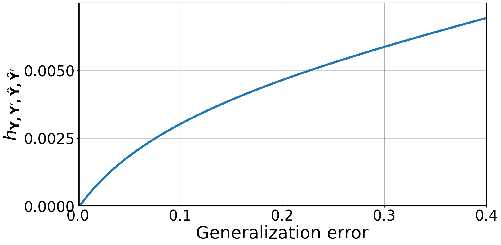
Figure 2: Values of $h_{C}\left(\mathcal{\hat{L}}(\mathbf{y},\mathbf{\hat{y}}),\mathcal{\hat{L}}(\mathbf{y}^{\prime},\mathbf{\hat{y}}^{\prime});\epsilon\right)$ for various values of the generalization error for the CIFAR10 dataset.

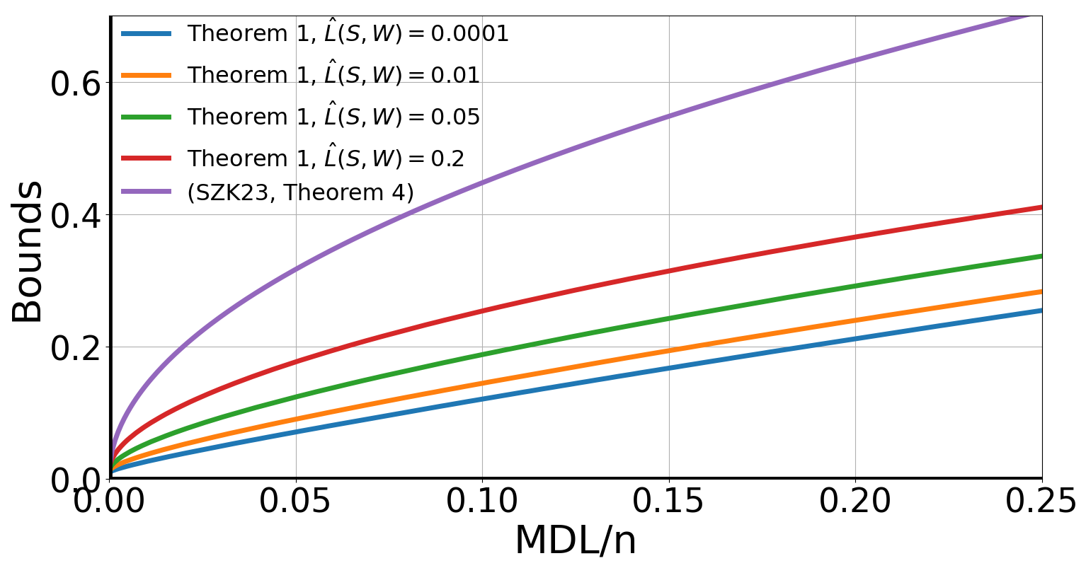
Figure 3: Comparison of the generalization bounds of Theorem 1 (for various values of $\hat{\mathcal{L}}(S,W)$) and [79, Theorem 4] for the CIFAR10 dataset.

3.2 Tail bound

The following theorem provides a probability tail bound on the generalization error of the representation learning setup of Fig. 1.

Theorem 2.

Consider the setup of Theorem 1 and consider some symmetric conditional distribution $\mathbf{Q}(\mathbf{U},\mathbf{U^{\prime}}|\mathbf{Y},\mathbf{Y^{\prime}},\mathbf{X},\mathbf{X^{\prime}},W_{e})$. Then, for any $\delta\geq 0$ and for $n\geq 10$, with probability at least $1-\delta$ over choices of $(S,S^{\prime},W)$, it holds that

$$h_{D}\left(\mathcal{\hat{L}}(S^{\prime},W),\mathcal{\hat{L}}(S,W)\right)\leq \frac{D_{KL}\left(P_{\mathbf{U},\mathbf{U}^{\prime}|\mathbf{X},\mathbf{X}^{\prime},W_{e}}\big{\|}\mathbf{Q}\ \right)+\log(n/\delta)}{n}$$

$$+\mathbb{E}_{\hat{\mathbf{Y}},\hat{\mathbf{Y}}^{\prime}|\mathbf{Y},\mathbf{Y}^{\prime}}\left[h_{\mathbf{Y},\mathbf{Y}^{\prime},\hat{\mathbf{Y}},\hat{\mathbf{Y}}^{\prime}}\left(\frac{1}{2}\left\|\hat{p}_{\mathbf{Y}}-\hat{p}_{\mathbf{Y}^{\prime}}\right\|_{1}\right)\right],$$ (13)

where $\hat{p}_{\mathbf{Y}}$ and $\hat{p}_{\mathbf{Y}^{\prime}}$ are empirical distributions of $\mathbf{Y}$ and $\mathbf{Y}^{\prime}$, respectively.

The proof of Theorem 2 appears in Appendix G.2.

3.3 Lossy generalization bounds

The bounds of the previous section can be regarded as lossless versions of ones that are more general, and which we refer to as lossy bounds. The lossy bounds are rather easy extensions of the corresponding lossless versions, but they have the advantage to be guaranteed to stay non-vacuous even when the encoder is set to be deterministic. Also, such bounds are useful to explain the empirically observed geometrical compression phenomenon [33]. For comparison, MI-based bounds, such Xu-Raginsky [89] are known to suffer both shortcomings [38; 60]. The aforementioned shortcomings have been shown that can be addressed using the lossy approach [78; 77]. For the sake of brevity, in the rest of this section we only illustrate how the bound (12) can be extended to a corresponding lossy one. Let $\hat{W}_{e}\in\mathcal{W}_{e}$ be any quantized model defined by $P_{\hat{W}_{e}|S}$, that satisfy the distortion criterion $\mathbb{E}_{P_{S,W}P_{\hat{W}_{e}|S}}\left[\operatorname{gen}(S,W)-\operatorname{gen}(S,\hat{W})\right]\leq\epsilon$, where $\hat{W}=(\hat{W}_{e},W_{d})$. Then, we get

$$\mathbb{E}_{\mathbf{S},W}\left[\operatorname{gen}(S,W)\right]\leq\sqrt{\frac{2\,\textnormal{MDL}(\mathbf{Q})+C+2}{n}}+\epsilon,$$ (14)

where now $\text{MDL}(\mathbf{Q})$ is considered for the quantized encoder, i.e.,

$$\textnormal{MDL}(\mathbf{Q})\coloneqq\mathbb{E}_{S,S^{\prime},\hat{W}_{e}}\Big{[}D_{KL}\Big{(}P_{\mathbf{U},\mathbf{U}^{\prime}|\mathbf{X},\mathbf{X}^{\prime},\hat{W}_{e}}\big{\|}\mathbf{Q}(\mathbf{U},\mathbf{U^{\prime}}|S,S^{\prime},\hat{W}_{e})\ \Big{)}\Big{]}.$$ (15)

4 Regularization using data-dependent Gaussian mixture priors

Theorems 1 and 2 essentially mean that if for a given learning algorithm the minimum description length $\textnormal{MDL}(\mathbf{Q})$ is small, then the algorithm is guaranteed to generalize well. Hence, it is natural to use the term $\textnormal{MDL}(\mathbf{Q})$ as a suitable regularizer. The question of the choice of the prior $\mathbf{Q}$ is pivotal for this. In this section, we propose an effective method to simultaneously find a data-dependent $\mathbf{Q}$ and use it to build a suitable regularizer term along the optimization iterations.

We assume that for a given input $x$ the encoder outputs the mean $\mu_{x}\in\mathbb{R}^{d}$ and standard deviation $\sigma_{x}\in\mathbb{R}^{d}$. Also, we assume that the latent variable $U$ is distributed according to a multivariate Gaussian distribution with a diagonal covariance matrix, i.e., $U\sim\mathcal{N}\big{(}\mu_{x},\operatorname{diag}(\sigma_{x}^{2})\big{)}$ where $\operatorname{diag}(\sigma_{x}^{2})$ denotes a $d\times d$ diagonal matrix with diagonal elements $\sigma_{x}^{2}$. With this assumption, we have

$$P_{\mathbf{U},\mathbf{U}^{\prime}|\mathbf{X},\mathbf{X}^{\prime},W_{e}}=\bigotimes\nolimits_{i\in[n]}\Big{\{}\mathcal{N}\big{(}\mu_{x_{i}},\operatorname{diag}(\sigma_{x_{i}}^{2})\big{)}\mathcal{N}\big{(}\mu_{x^{\prime}_{i}},\operatorname{diag}(\sigma_{x^{\prime}_{i}}^{2})\big{)}\Big{\}}.$$

In our approach, we model the prior $\mathbf{Q}$ as a suitable Gaussian mixture, with the mixture coefficients chosen judiciously in a manner that is training-data dependent and along the optimization iterations. The rationale for this choice is two-fold: (i) The Gaussian mixture distribution is known to possibly approximate well enough any arbitrary distribution provided that the number of mixture components is sufficiently large [21; 36] (see also [68, Theorem 1]); and (ii) given distributions $\{p_{i}\}_{i\in[N]}$, the distribution $q$ that minimizes $\sum_{i\in[N]}D_{KL}(p_{i}\|q)$ is $q=\frac{1}{N}\sum_{i\in[N]}p_{i}$. Thus, if all distributions $p_{i}$ are Gaussian, the minimizer is a Gaussian mixture.

Let, for $c\in[C]$, $Q_{c}$ denote the data-dependent Gaussian mixture prior $Q_{c}$ for label $c$. Also, let $\mathbf{Q}(\mathbf{U},\mathbf{U^{\prime}}|S,S^{\prime},\hat{W}_{e})=\prod_{i\in[n]}Q_{Y_{i}}(U_{i})Q_{Y^{\prime}_{i}}(U^{\prime}_{i})$. It is easy to see that this prior satisfies the symmetry property of Definition 1. In what follows, we explain how the priors $\{Q_{c}\}$ are chosen and updated along the optimization iterations. As it will become clearer, our method is somewhat reminiscent of the expectation-maximization (EM) algorithm for finding Gaussian mixture priors that maximize the log-likelihood, but with notable major differences: (i) In our case the prior must be learned along the optimization iterations with the underlying distribution of the latent variables possibly changing at every iteration. (ii) The Gaussian mixture prior is intended to be used in a regularizer term, not to maximize the log-likelihood; and, hence, the approach must be adapted accordingly. (iii) Unlike the usual scenario where the goal is to find an appropriate Gaussian mixture given a set of points, here we are given a set of distributions i.e., $\mathcal{N}\left(\mu_{x_{i}},\operatorname{diag}(\sigma_{x_{i}}^{2})\right)$ that generate such points. (iv) The found prior must satisfy (at least partially) certain “symmetry” properties.

4.1 Lossless Gaussian mixture prior

For each label $c\in[C]$, we let the prior $Q_{c}$ to be defined as

$$Q_{c}=\sum\nolimits_{m\in[M]}\alpha_{c,m}\,Q_{c,m},$$ (16)

over $\mathbb{R}^{d}$, where $\alpha_{c,m}\in[0,1]$, $\sum_{m\in[M]}\alpha_{c,m}=1$ for each $c\in[C]$, and where $\{Q_{c,m}\}_{c,m}$ are multivariate Gaussian distributions with a diagonal covariance matrix:

$$Q_{c,m}=\mathcal{N}\left(\mu_{c,m},\operatorname{diag}\left(\sigma_{c,m}^{2}\right)\right),\quad m\in[M],c\in[C].$$

With the above prior choice, the regularizer term simplifies as $\sum\nolimits_{i\in[b]}D_{KL}\big{(}P_{U_{i}|X_{i},W_{e}}\big{\|}Q_{Y_{i}}\big{)}$. However, since the KL-divergence between a Gaussian and a Gaussian mixture distributions does not have a closed-form expression, we estimate it using a slightly adapted method from [45]. Our estimate is an average of the upper and lower bounds of the KL-divergence, denoted as $D_{\text{var}}$ and $D_{\text{prod}}$. Please refer to Appendix F for more details on this estimation. For better readability, we present the approximation of the KL-divergence by its upper bound $D_{\text{var}}$ in the main part of this paper and we refer the reader to Appendix C for the approach using $\big{(}D_{\text{var}}+D_{\text{prod}}\big{)}/2$.

Finally, similar to [3; 79], we consider only the part of the upper bound $\textnormal{MDL}(\mathbf{Q})$ corresponding to the training dataset $S$, simply because the test dataset $S^{\prime}$ is not available during the training phase. With this assumption and for a mini-batch $\mathcal{B}=\{z_{1},\ldots,z_{b}\}\subseteq S$, the regularizer term is equal to

$$\textnormal{Regularizer}(\mathbf{Q})\coloneqq D_{KL}\big{(}P_{\mathbf{U}_{\mathcal{B}}|\mathbf{X}_{\mathcal{B}},W_{e}}\big{\|}\mathbf{Q}_{\mathcal{B}}\ \big{)},$$ (17)

where the indices $\mathcal{B}$ indicate the restriction to the set $\mathcal{B}$. For better exposition, we will drop the notation dependence on $\mathcal{B}$ in the rest of this section. Now, we are ready to explain how the Gaussian mixtures are initialized, updated, and used as a regularizer simultaneously and along the optimization iterations. In what follows, the superscript $(t)$ denotes the optimization iteration $t\in\mathbb{N}^{*}$.

Initialization. First, we initialize the priors as $Q_{c}^{(0)}$ by initializing $\alpha_{c,m}^{(0)}$ and the parameters $\mu_{c,m}^{(0)}$ $\sigma_{c,m}^{(0)}$ of the components $Q_{c,m}^{(0)}$, for $c\in[C],m\in[M]$, similar to the method of initializing the centers in k-means++ [8]. The reader is referred to Appendix C.1 for further details.

Update of the priors. Let the mini-batch picked at iteration $t$ be $\mathcal{B}^{(t)}=\{z_{1}^{(t)},\ldots,z_{b}^{(t)}\}$. By dropping the dependence on $(t)$ for better readability, the regularizer 17, at iteration $(t)$, can be written as

$$\textnormal{Regularizer}(\mathbf{Q})= \sum\nolimits_{i\in[b]}D_{KL}\big{(}P_{U_{i}|x_{i},w_{e}}\big{\|}\sum\nolimits_{m\in[M]}\alpha_{y_{i},m}^{(t)}Q^{(t)}_{y_{i},m}(U_{i})\big{)}$$

$$\stackrel{{\scriptstyle(a)}}{{\leq}} \sum\limits_{i\in[b]}\sum\limits_{m\in[M]}\gamma_{i,m}\left(D_{KL}\big{(}P_{U_{i}|x_{i},w_{e}}\big{\|}Q^{(t)}_{y_{i},m}(U_{i})\big{)}-\log\big{(}\alpha_{y_{i},m}^{(t)}/\gamma_{i,m}\big{)}\right),$$ (18)

where the last step holds for any choices of $\gamma_{i,m}\geq 0$ such that $\sum_{m\in[M]}\gamma_{i,m}=1$, for every $i\in[b]$. To see why the step $(a)$ holds, we refer the reader to Appendix F to see how the variational bound $D_{var}$ is derived.

Now, to update the components of the priors, first (similar to ‘E’-step) note that the coefficients $\gamma_{i,m}$ that minimizes the above upper bound are equal to

$$\gamma_{i,m}=\frac{\alpha_{y_{i},m}^{(t)}e^{-D_{KL}\big{(}P_{U_{i}|x_{i},w_{e}}\|Q_{y_{i},m}^{(t)}\big{)}}}{\sum\nolimits_{m^{\prime}\in[M]}\alpha_{y_{i},m^{\prime}}^{(t)}e^{-D_{KL}\big{(}P_{U_{i}|x_{i},w_{e}}\|Q_{y_{i},m^{\prime}}^{(t)}\big{)}}},\quad i\in[b],m\in[M].$$ (19)

Let $\gamma_{i,c,m}=\gamma_{i,m}$ if $c=y_{i}$ and $\gamma_{i,c,m}=0$ otherwise. Next, (similar to $M$-step) we treat $\gamma_{i,m}$ as constants, and find the parameters $\mu_{c,m}^{*}$, $\sigma^{*}_{c,m,j}$, $\alpha_{c,m}^{*}$ that minimizes the upper bound (18), by simply taking the partial derivatives and equating them to zero. Simple calculations show that the closed-form solutions are

$$\mu_{c,m}^{*}= \frac{1}{b_{c,m}}\sum\nolimits_{i\in[b]}\gamma_{i,c,m}\mu_{x_{i}}, {\sigma^{*}_{c,m,j}}^{2}=\frac{1}{b_{c,m}}\sum\nolimits_{i\in[b]}\gamma_{i,c,m}\left(\sigma_{x_{i},j}^{2}+(\mu_{x_{i},j}-\mu_{c,m,j}^{(t)})^{2}\right),$$

$$\alpha_{c,m}^{*}= b_{c,m}/b_{c},\quad b_{c,m}=\sum\nolimits_{i\in[b]}\gamma_{i,c,m},\quad\quad b_{c}=\sum\nolimits_{m\in[M]}b_{c,m}.\hskip 42.67912pt$$ (20)

where $j\in[d]$ denotes the index of the coordinate in $\mathbb{R}^{d}$ and $\sigma_{c,m}^{*}=(\sigma_{c,m,1}^{*},\ldots,\sigma_{c,m,d}^{*})$. Finally, to reduce the dependence of the prior on the dataset and to partially preserve the symmetry property, let

$$\mu_{c,m}^{(t+1)}= (1-\eta_{1})\mu_{c,m}^{(t)}+\eta_{1}\mu_{c,m}^{*}+\mathfrak{Z}_{1}^{(t+1)},\quad{\sigma_{c,m}^{(t+1)}}^{2}=(1-\eta_{2}){\sigma_{c,m}^{(t)}}^{2}+\eta_{2}{\sigma_{c,m}^{*}}^{2}+\mathfrak{Z}_{2}^{(t+1)},$$

$$\alpha_{c,m}^{(t+1)}= (1-\eta_{3})\alpha_{c,m}^{(t)}+\eta_{3}\alpha_{c,m}^{*},$$ (21)

where $\eta_{1},\eta_{2},\eta_{3}\in[0,1]$ are some fixed coefficients and $\mathfrak{Z}_{j}^{(t+1)}$, $j\in[2]$, are i.i.d. multivariate Gaussian random variables distributed as $\mathcal{N}(\mathbf{0}_{d},\zeta_{j}^{(t+1)}\mathrm{I}_{d})$. Here $\mathbf{0}_{d}=(0,\ldots,0)\in\mathbb{R}^{d}$ and $\zeta_{j}^{(t+1)}\in\mathbb{R}^{+}$ are some fixed constants.

Regularizer. Finally, using (19), the upper bound (18) that we use as a regularizer, can be simplified as

$$-\sum\nolimits_{i\in[b]}\log\Big{(}\sum\nolimits_{m\in[M]}\alpha_{y_{i},m}^{(t)}e^{-D_{KL}\big{(}P_{U_{i}|x_{i},w_{e}}\|Q_{y_{i},m}^{(t)}\big{)}}\Big{)}.$$ (22)

4.2 Lossy Gaussian mixture prior

The lossy case is explained in Appendix C.3 when the KL-divergence estimate $\left(D_{\text{prod}}+D_{\text{var}}\right)/2$ is considered. Similar to Section 4.1, it can be shown that if only $D_{\text{var}}$ is considered for the KL-divergence estimate, then the regularizer term becomes equal to

$$-\sum\nolimits_{i\in[b]}\log\left(\sum\nolimits_{m\in[M]}\alpha_{y_{i},m}^{(t)}e^{-D_{KL,Lossy}\big{(}P_{U_{i}|x_{i},\hat{w}_{e}}\|Q_{y_{i},m}^{(t)}\big{)}}\right),$$ (23)

where $D_{KL,Lossy}\big{(}P_{U|x,\hat{w}_{e}}\|Q_{y,m}\big{)}$ is defined as

$${D_{KL}}\bigg{(}\mathcal{N}\bigg{(}\mu_{x},\frac{\sqrt{d}}{2}\mathrm{I}_{d}\bigg{)}\Big{\|}\mathcal{N}\bigg{(}\mu_{c,m},\frac{\sqrt{d}}{2}\mathrm{I}_{d}\bigg{)}\bigg{)}{+}D_{KL}\Big{(}\mathcal{N}\big{(}\mathbf{0}_{d},\operatorname{diag}(\sigma_{x}^{2}{+}\boldsymbol{\epsilon})\big{)}\big{\|}\mathcal{N}\big{(}\mathbf{0}_{d},\operatorname{diag}(\sigma_{c,m}^{2}{+}\boldsymbol{\epsilon})\big{)}\Big{)},$$ (24)

where $\boldsymbol{\epsilon}=(\epsilon,\ldots,\epsilon)\in\mathbb{R}^{d}$ and $\epsilon\in\mathbb{R}^{+}$ is a fixed hyperparameter.

Furthermore the components are updated according to (21), where $\gamma_{i,c,m}$, $\mu_{c,m}^{*}$, and $\alpha_{c,m}^{*}$ are defined as before, but ${\sigma^{*}_{c,m,j}}^{2}=\frac{1}{b_{c,m}}\sum\nolimits_{i\in[b]}\gamma_{i,c,m}\sigma_{x_{i},j}^{2}$ and $\gamma_{i,m}$ is equal to

$$\gamma_{i,m}= \frac{\alpha_{y_{i},m}^{(t)}e^{-D_{KL,Lossy}\big{(}P_{U_{i}|x_{i},\hat{w}_{e}}\|Q_{y_{i},m}^{(t)}\big{)}}}{\sum\nolimits_{m^{\prime}\in[M]}\alpha_{y_{i},m^{\prime}}^{(t)}e^{-D_{KL,Lossy}\big{(}P_{U_{i}|x_{i},\hat{w}_{e}}\|Q_{y_{i},m^{\prime}}^{(t)}\big{)}}}=\frac{\beta_{y_{i},m}^{(t)}e^{\frac{\langle\mu_{x_{i}},\mu_{y_{i},m}^{(t)}\rangle}{\sqrt{d}}}}{\sum\nolimits_{m^{\prime}\in[M]}\beta_{y_{i},m^{\prime}}^{(t)}e^{\frac{\langle\mu_{x_{i}},\mu_{y_{i},m^{\prime}}^{(t)}\rangle}{\sqrt{d}}}},$$

where $\beta_{y_{i},m}^{(t)}=\alpha_{y_{i},m}^{(t)}e^{-\frac{\|\mu_{y_{i},m}^{(t)}\|^{2}}{\sqrt{d}}}e^{-\sum_{j\in[d]}(\log(\sigma_{y_{i},m,j}^{(t)}/\sigma_{x_{i},j})+\sigma_{x_{i},j}^{2}/(2{\sigma_{y_{i},m,j}^{(t)}}^{2}))}$. In cases where the means of the components are normalized and the variances are fixed, $\beta_{y_{i},m}^{(t)}\propto\alpha_{y_{i},m}^{(t)}$.

The parameters $\gamma_{i,m}$ measure the contribution of the component $m$ in $Q_{y_{i}}$ in generating the latent variable $U_{i}$. One can observe a similarity between how these parameters are chosen in our approach and the attention mechanism, with the difference that here we are considering a weighted version of this mechanism, and without key and query matrices since we do not consider projections to other spaces. Intuitively, to measure the contribution of each component, we measure how much that component “attend” to $U_{i}$.

5 Experiments

In this section, we present the results of our simulations. The reader is referred to Appendix E for additional details, including used datasets, models, and training hyperparameters.

For the experiments, we considered the lossy regularizer approach with Gaussian mixture prior and the KL-divergence estimate of $\left(D_{\text{prod}}+D_{\text{var}}\right)/2$, as detailed in Appendix C.3. In this section, we refer to our regularizer as Gaussian mixture MDL (GM-MDL). To verify the practical benefits of the introduced regularizer, we conducted several experiments considering different datasets and encoder architectures as summarized below and detailed in Appendix E:

• Datasets: CIFAR10, CIFAR100, INTEL, and USPS image classification,

• Encoder architectures: CNN4 and ResNet18.

To compare our approach with the previous literature, in addition to the no-regularizer case, we also considered the Variational Information Bottleneck (VIB) of [3] and the Category-dependent VIB (CDVIB) of [79].

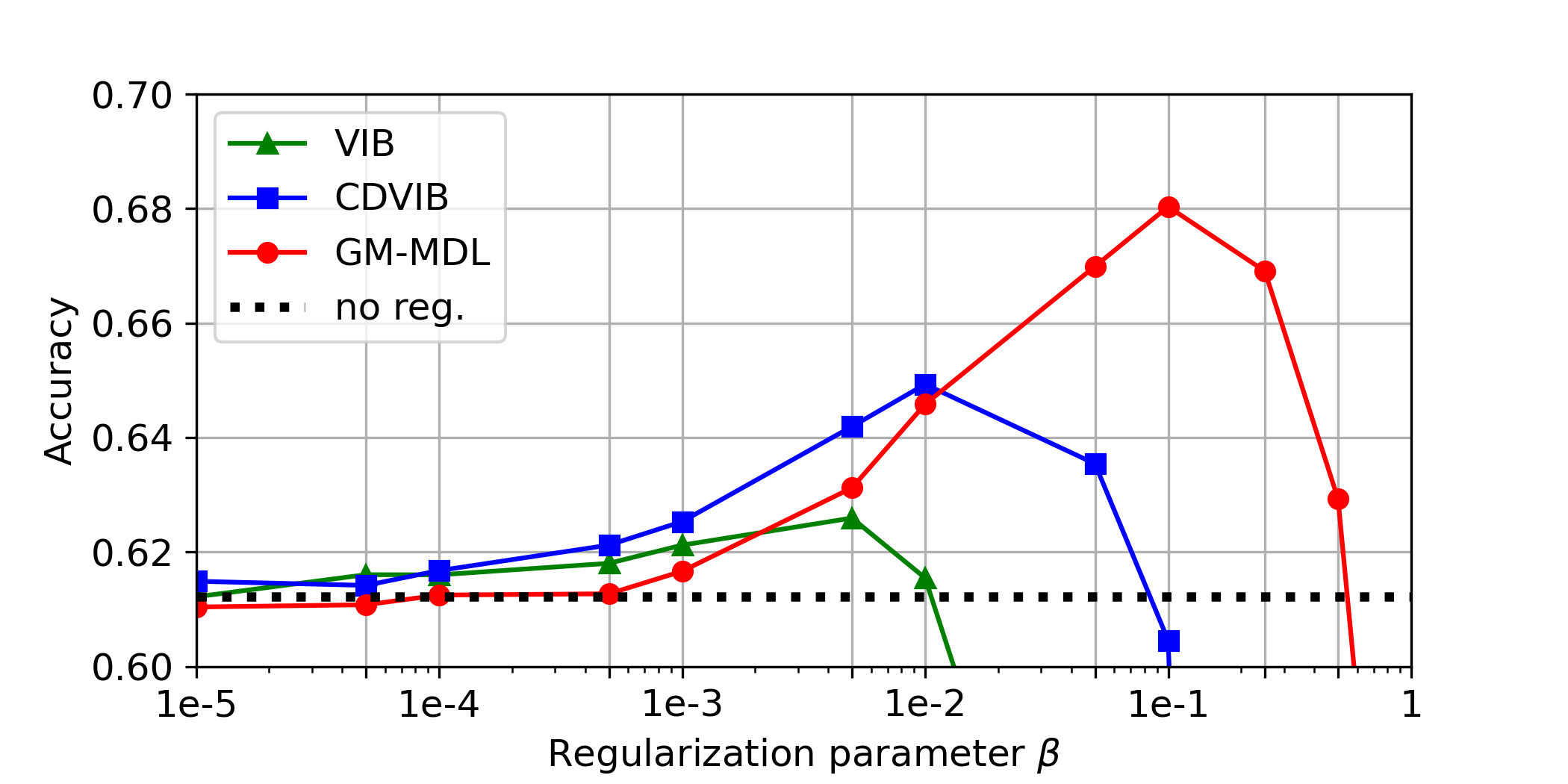
Figure 4: Test performance of the CNN-based encoder trained on CIFAR10 using standard VIB [3] regularization, Category-dependent VIB (CDVIB) [79] regularization, and our proposed Gaussian Mixture MDL (GM-MDL) regularization.

The results presented in Fig. 4 and Table 1 clearly show the practical advantages of our proposed approach. All experiments are run independently for 5 times and the reported values and plots are the average over 5 runs. In Fig.4, we plotted the performance of different regularizers as a function of the trade-off regularization parameter $\beta$. In Table 1, we reported the best achieved average test accuracy for each regularizer.

Table 1: Test performance of representation learning models with different encoder architectures, and trained on selected datasets using VIB [3], Category-dependent VIB (CDVIB) [79], and our proposed Gaussian Mixture MDL (GM-MDL).

#	Encoder	Dataset	no reg.	VIB	CDVIB	GM-MDL
1	CNN4	CIFAR10	0.612	0.626	0.649	0.681
2	CNN4	USPS	0.948	0.952	0.955	0.963
3	CNN4	INTEL	0.756	0.759	0.763	0.776
4	ResNet18	CIFAR10	0.824	0.829	0.835	0.848
5	ResNet18	CIFAR100	0.454	0.458	0.463	0.497

Appendices

The appendices are organized as follows:

• In Appendix A, we provide the intuition behind the lossy generalization bounds and we present an extension of Theorem 1 to lossy compression settings.

• In Appendix B, we show how the established generalization bounds of this work can be extended to cases where the prior violates the symmetry condition.

• In Appendix C, we explain in detail our approach to finding the Gaussian mixture and Gaussian-product mixture priors and how to use them in a regularizer term. This subsection is further divided into three parts, describing

  • our initialization method in Appendix C.1,

  • the lossless approach in Appendix C.2,

  • and the lossy approach in Appendix C.3.

• In Appendix D, we discuss the potential future directions.

• Appendix E explains the details of our experiments.

• Appendix F contains the used approximation method for the KL divergence between a Gaussian distribution and a Gaussian mixture distribution, and also between two Gaussian mixture distributions.

• Finally, the deferred proofs are presented in Appendix G.

Appendix A Intuition behind lossy generalization bounds

The bounds of Theorems 1 and 2 for the deterministic encoders may become vacuous, due to the KL-divergence term, and the bounds cannot explain the empirically observed geometrical compression phenomenon [Geiger, 2021]. These issues can be addressed using the lossy compressibility approach, as opposed to the lossless compressibility approach considered in previous sections. To provide a better intuition for these approaches, we first briefly explain their counterparts in information theory, i.e., lossless and lossy source compression.

Consider a discrete source $V\sim P_{V}$ and assume that we have $n$ i.i.d. realizations $V_{1},\ldots,V_{n}$ of this source. Then, for sufficiently large values of $n$, the classical lossless source coding result in information theory states that this sequence can be described by approximately $nH(V)$ bits, where $H(V)$ is the Shannon entropy function. Thus, intuitively, $H(V)$ is the complexity of the source $V$. Now suppose that $V$ is no longer discrete. Then $V_{1},\ldots,V_{n}$ can no longer be described by any finite number of bits. However, if we consider some “vector quantization” instead, a sufficiently close vector can be described by a finite number of bits. This concept is called lossy compression. The amount of closeness is called the distortion, and the minimum number of needed bits (per sample) to describe the source within a given distortion level is given by the rate-distortion function.

Similar to [Sefidgaran et al., 2023, Section 2.2.1 and Appendix C.1.2], we borrow such concepts to capture the “lossy complexity” of the latent variables in order to avoid non-vacuous bounds which can also explain the geometrical compression phenomenon [Geiger, 2021, Sefidgaran et al., 2023]. This is achieved by considering the compressibility of “quantized” latent variables derived using the “distorted” encoders $\hat{W}_{e}$. Note that $\hat{W}_{e}$ is distorted only for the regularization term to measure the lossy compressibility (rate-distortion), and the undistorted latent variables are passed to the decoder. This is different from approaches that simply add noise to the output of the encoder and pass it to the decoder.

Finally, we show how to derive similar lossy bounds to (14) in terms of the function $h_{D}$. We first define the inverse of the function $h_{D}$ as follows. For any $y\in[0,2]$ and $x_{2}\in[0,1]$, let

$$h_{D}^{-1}(y|x_{2})=\sup\left\{x_{1}\in[0,1]\colon h_{D}(x_{1},x_{2})\leq y\right\}.$$ (25)

Let $\hat{W}_{e}\in\mathcal{W}_{e}$ be any quantized model defined by $P_{\hat{W}_{e}|S}$, that satisfy the distortion criterion $\mathbb{E}_{P_{S,W}P_{\hat{W}_{e}|S}}\left[\operatorname{gen}(S,W)-\operatorname{gen}(S,\hat{W})\right]\leq\epsilon$, where $\hat{W}=(\hat{W}_{e},W_{d})$. Then, using Theorem 1 for the quantized model, we have

$$\mathbb{E}_{\mathbf{S},\mathbf{S}^{\prime},\hat{W},\hat{\mathbf{Y}},\hat{\mathbf{Y}}^{\prime}}\Big{[}h_{D}\Big{(} \mathcal{\hat{L}}(\mathbf{Y}^{\prime},\mathbf{\hat{Y}}^{\prime}),\mathcal{\hat{L}}(\mathbf{Y},\mathbf{\hat{Y}})\Big{)}\Big{]}\leq$$

$$\frac{\,\textnormal{MDL}(\mathbf{Q})+\log(n)}{n}+\mathbb{E}_{\mathbf{Y},\mathbf{Y}^{\prime},\hat{\mathbf{Y}},\hat{\mathbf{Y}}^{\prime}}\left[h_{\mathbf{Y},\mathbf{Y}^{\prime},\hat{\mathbf{Y}},\hat{\mathbf{Y}}^{\prime}}\left(\frac{1}{2}\left\|\hat{p}_{\mathbf{Y}}-\hat{p}_{\mathbf{Y}^{\prime}}\right\|_{1}\right)\right]\eqqcolon\Delta(\hat{W},\mathbf{Q}).$$ (26)

Next, using the Jensen inequality we have

$$h_{D}\Big{(}\mathbb{E}_{\hat{W}}[\mathcal{L}(\hat{W})],\mathbb{E}_{S,\hat{W}}[\hat{\mathcal{L}}(S,\hat{W})]\Big{)}\Big{]}\leq\mathbb{E}_{\mathbf{S},\mathbf{S}^{\prime},\hat{W},\hat{\mathbf{Y}},\hat{\mathbf{Y}}^{\prime}}\Big{[}h_{D}\Big{(}\mathcal{\hat{L}}(\mathbf{Y}^{\prime},\mathbf{\hat{Y}}^{\prime}),\mathcal{\hat{L}}(\mathbf{Y},\mathbf{\hat{Y}})\Big{)}\Big{]}.$$ (27)

Combining the above two inequalities yields

$$h_{D}\Big{(}\mathbb{E}_{\hat{W}}[\mathcal{L}(\hat{W})],\mathbb{E}_{S,\hat{W}}[\hat{\mathcal{L}}(S,\hat{W})]\Big{)}\Big{]}\leq\Delta(\hat{W},\mathbf{Q}).$$ (28)

Finally, we have

$$\mathbb{E}_{\mathbf{S},W}\left[\operatorname{gen}(S,W)\right]\leq \mathbb{E}_{\mathbf{S},\hat{W}}\left[\operatorname{gen}(S,\hat{W})\right]+\epsilon$$

$$= \mathbb{E}_{\hat{W}}[\mathcal{L}(\hat{W})]-\mathbb{E}_{S,\hat{W}}[\hat{\mathcal{L}}(S,\hat{W})]+\epsilon$$

$$\leq h_{D}^{-1}\left(\min(2,\Delta(\hat{W},\mathbf{Q}))\big{|}\mathbb{E}_{S,\hat{W}}[\hat{\mathcal{L}}(S,\hat{W})]\right)-\mathbb{E}_{S,\hat{W}}[\hat{\mathcal{L}}(S,\hat{W})]+\epsilon$$ (29)

In particular, for negligible values of $\mathbb{E}_{S,\hat{W}}[\hat{\mathcal{L}}(S,\hat{W})]$, $h_{D}^{-1}\left(\min(2,\Delta(\hat{W},\mathbf{Q}))\big{|}\mathbb{E}_{S,\hat{W}}[\hat{\mathcal{L}}(S,\hat{W})]\right)\approx\min(2,\Delta(\hat{W},\mathbf{Q}))\lesssim\frac{\textnormal{MDL}(\mathbf{Q})+\log(n)}{n}$, which gives

$$\mathbb{E}_{\mathbf{S},W}\left[\operatorname{gen}(S,W)\right]\lesssim\frac{\textnormal{MDL}(\mathbf{Q})+\log(n)}{n}+\epsilon.$$

Appendix B Generalization bounds via non-symmetric priors

In this section, we discuss how the bounds of Theorems 1 and 2 can be extended to settings in which the requirement of symmetry is relaxed partially. We focus on “differentially private” and “partially symmetric” data-dependent priors.

B.1 Differentially private data-dependent priors

One way to extend the results to include the partially symmetric data-dependent priors is by leveraging the differential privacy tools [Dwork, 2006, Dwork et al., 2014, 2015, Dziugaite and Roy, 2018]. The reader is referred to [Alquier, 2021, Section 3.3] for more on differentially private priors.

Recall that given the dataset $S$ we train a model $W$ using the learning algorithm $\mathcal{A}(\cdot)$, i.e., $W=\mathcal{A}(S)$. Now, assume that by having the dataset $S$ and the trained model $W=\mathcal{A}(S)$ we choose the prior $\mathbf{Q}^{S,W}$ using a potentially stochastic mechanism $\mathcal{T}\colon\mathcal{S}\times\mathcal{W}\to\mathcal{Q}$, where $\mathcal{Q}$ denotes the space of all conditional distributions of $\mathbf{U},\mathbf{U^{\prime}}$ given $(\mathbf{Y},\mathbf{Y}^{\prime})$, that is “strongly” symmetric. To state the definition of strongly symmetric prior, we first recall the notations of $\mathbf{U}_{\pi},\mathbf{U^{\prime}}_{\pi}$ and $\mathbf{Y}_{\pi},\mathbf{Y}^{\prime}_{\pi}$ for any permutation $\pi:[2n]\to[2n]$. Let $Y^{2n}\coloneqq(\mathbf{Y},\mathbf{Y}^{\prime})$. Then, we define $\mathbf{Y}_{\pi}$ and $\mathbf{Y}^{\prime}_{\pi}$ as

$$\mathbf{Y}_{\pi}\coloneqq Y_{\pi(1)},\ldots,Y_{\pi(n)},$$

$$\mathbf{Y}_{\pi}\coloneqq Y_{\pi(n+1)},\ldots,Y_{\pi(2n)}.$$ (30)

The variables $\mathbf{U}_{\pi}$ and $\mathbf{U^{\prime}}_{\pi}$ are defined in a similar manner.

Definition 2 (Strongly symmetric prior).

A conditional distribution $\mathbf{Q}$ of $\mathbf{U},\mathbf{U^{\prime}}$ given $(\mathbf{Y},\mathbf{Y}^{\prime})$ is strongly symmetric, if for every $(\mathbf{U},\mathbf{U^{\prime}},\mathbf{Y},\mathbf{Y}^{\prime})$ and every permutation $\pi\colon[2n]\to[2n]$ that preserves the labeling (i.e., $\mathbf{Y}_{\pi}=\mathbf{Y}$ and $\mathbf{Y}^{\prime}_{\pi}=\mathbf{Y}^{\prime}$) we have

$$\mathbf{Q}\left(\mathbf{U},\mathbf{U^{\prime}}|\mathbf{Y},\mathbf{Y}^{\prime}\right)= \mathbf{Q}\left(\mathbf{U}_{\pi},\mathbf{U^{\prime}}_{\pi}|\mathbf{Y},\mathbf{Y}^{\prime}\right).$$ (31)

Note that any strongly symmetric prior satisfies the symmetry condition of Definition 1. In addition, the per-label Gaussian-mixture prior of Section 4 meets the strongly symmetric condition. To show this, recall that for any $c\in[C]$, the Gaussian mixture prior for label $c$ is denoted by $Q_{c}$. Given these per-label priors, the prior $\mathbf{Q}$ is defined as

$$\mathbf{Q}(\mathbf{U},\mathbf{U^{\prime}}|S,S^{\prime},\hat{W}_{e})= \mathbf{Q}(\mathbf{U},\mathbf{U^{\prime}}|\mathbf{Y},\mathbf{Y}^{\prime})$$

$$= \prod_{i\in[n]}Q_{Y_{i}}(U_{i})Q_{Y^{\prime}_{i}}(U^{\prime}_{i}).$$

It is immediate to see that this prior is strongly symmetric under any permutation that preserves the labeling.

Next, we define the notion of learning the prior in a differentially private manner. For simplicity, we consider the case where $\mathcal{A}(S)$ can be written as a deterministic function $g(S,V)$, where $V$ represents all the stochasticity in the learning algorithm that is independent of $S$. An example of such a learning algorithm is the Stochastic Gradient Descent (SGD) algorithm.

Definition 3 (Differentially private prior).

We say $\mathcal{T}\colon\mathcal{S}\times\mathcal{W}\to\mathcal{Q}$ is $\varepsilon_{p}$-differentially private if for any fixed $V$, and all datasets $S$ and $S_{1}$ that are different in only one coordinate and for all measurable subsets $B\subseteq\mathcal{Q}$, we have

$$\mathbb{P}\left(\mathbf{Q}^{S,\mathcal{A}(S)}\in B\right)\leq e^{\varepsilon_{p}}\mathbb{P}\left(\mathbf{Q}^{S_{1},\mathcal{A}(S_{1})}\in B\right),$$ (32)

where $\mathcal{A}(S)=g(S,V)$ and $\mathcal{A}(S_{1})=g(S_{1},V)$.

Now, we state our tail-bound result for $\varepsilon_{p}$-differentially private prior.

Proposition 1.

Consider the setup of Theorem 1 and suppose the prior $\mathbf{Q}^{S,\mathcal{A}(S)}$ is chosen using an $\varepsilon_{p}$-differentially private mechanism $\mathcal{T}\colon\mathcal{S}\times\mathcal{W}\to\mathcal{Q}$. Then, for any $\delta\geq 0$ and for $n\geq 10$, with probability at least $1-\delta$ over choices of $(S,S^{\prime},W)$, it holds that

$$h_{D}\left(\mathcal{\hat{L}}(S^{\prime},W),\mathcal{\hat{L}}(S,W)\right)\leq \frac{D_{KL}\left(P_{\mathbf{U},\mathbf{U}^{\prime}|\mathbf{X},\mathbf{X}^{\prime},W_{e}}\big{\|}\mathbf{Q}^{S,\mathcal{A}(S)}\ \right)+\log(2n/\delta)}{n}$$

$$+\mathbb{E}_{\hat{\mathbf{Y}},\hat{\mathbf{Y}}^{\prime}|\mathbf{Y},\mathbf{Y}^{\prime}}\left[h_{\mathbf{Y},\mathbf{Y}^{\prime},\hat{\mathbf{Y}},\hat{\mathbf{Y}}^{\prime}}\left(\frac{1}{2}\left\|\hat{p}_{\mathbf{Y}}-\hat{p}_{\mathbf{Y}^{\prime}}\right\|_{1}\right)\right]$$

$$+\frac{1}{2}\varepsilon_{p}^{2}+\varepsilon_{p}\sqrt{\frac{\log(4/\delta)}{2n}},$$ (33)

where $\hat{p}_{\mathbf{Y}}$ and $\hat{p}_{\mathbf{Y}^{\prime}}$ are empirical distributions of $\mathbf{Y}$ and $\mathbf{Y}^{\prime}$, respectively.

The proof stated in Appendix G.3 is an extension of Theorem 2 using [Dwork et al., 2015, Theorems 18&19] and [Dziugaite and Roy, 2018, Theorem 4.2].

B.2 Partially symmetric data-dependent priors

In this section, we show an alternative way to extend our generalization bound results by defining the partially symmetric priors.

Definition 4 (Partially symmetric prior).

The prior $\mathbf{Q}$ is $(\epsilon,\delta)$-partially symmetric for the learning algorithm $\mathcal{A}\colon\mathcal{Z}^{n}\to\mathcal{W}$, if with probability at least $1-\delta$ over choices of $(S^{\prime},S,W_{e},\mathbf{U},\mathbf{U^{\prime}})\sim P_{S^{\prime}}P_{S,W_{e}}\mathbf{Q}$,

$$\forall\pi_{\mathbf{Y},\mathbf{Y}^{\prime}}\colon\quad\mathbf{Q}(\mathbf{U},\mathbf{U^{\prime}}|\mathbf{Y},\mathbf{Y^{\prime}},\mathbf{X},\mathbf{X^{\prime}},W_{e})\leq e^{\epsilon}\mathbf{Q}(\mathbf{U}_{\pi_{\mathbf{Y},\mathbf{Y}^{\prime}}},\mathbf{U^{\prime}}_{\pi_{\mathbf{Y},\mathbf{Y}^{\prime}}}|\mathbf{Y},\mathbf{Y^{\prime}},\mathbf{X},\mathbf{X^{\prime}},W_{e}),$$ (34)

where this should hold for any permutation $\pi_{\mathbf{Y},\mathbf{Y}^{\prime}}$ (which could potentially depend on $\mathbf{Y},\mathbf{Y}^{\prime}$) that satisfies the labeling.

Note that the partially symmetric prior can potentially depend on $(S,W)$.

Proposition 2.

Consider the setup of Theorem 1. Then, for any $(\epsilon,\delta)$-partially symmetric conditional distribution $\mathbf{Q}$ and for $n\geq 10$, we have

$$\mathbb{E}_{\mathbf{S},\mathbf{S}^{\prime},W,\hat{\mathbf{Y}},\hat{\mathbf{Y}}^{\prime}}\Big{[}h_{D}\Big{(}\mathcal{\hat{L}}(\mathbf{Y}^{\prime},\mathbf{\hat{Y}}^{\prime}),\mathcal{\hat{L}}(\mathbf{Y},\mathbf{\hat{Y}})\Big{)}\Big{]}\leq \frac{\,\textnormal{MDL}(\mathbf{Q})+\log\big{(}\delta e^{2n}+ne^{\epsilon}\big{)}}{n}$$

$$+\mathbb{E}_{\mathbf{Y},\mathbf{Y}^{\prime},\hat{\mathbf{Y}},\hat{\mathbf{Y}}^{\prime}}\left[h_{\mathbf{Y},\mathbf{Y}^{\prime},\hat{\mathbf{Y}},\hat{\mathbf{Y}}^{\prime}}\left(\frac{1}{2}\left\|\hat{p}_{\mathbf{Y}}-\hat{p}_{\mathbf{Y}^{\prime}}\right\|_{1}\right)\right].$$ (35)

where $\hat{p}_{\mathbf{Y}}$ and $\hat{p}_{\mathbf{Y}^{\prime}}$ are empirical distributions of $\mathbf{Y}$ and $\mathbf{Y}^{\prime}$, respectively and $\textnormal{MDL}(\mathbf{Q})$ is defined in 10.

This result is proved in Appendix G.4.

Appendix C Gaussian-productss mixture prior approximation and regularization

In this section, we explain in detail our approach to finding an appropriate data-dependent Gaussian mixture prior and how to use it in a regularizer term along the optimization trajectories. The section is subdivided into three parts: the first part explains how we initialize the components of the Gaussian mixture prior, and the other two parts explain the lossless and lossy versions of our approach.

Recall that we are considering a regularizer term equal to

$$\textnormal{Regularizer}(\mathbf{Q})\coloneqq D_{KL}\big{(}P_{\mathbf{U}_{\mathcal{B}}|\mathbf{X}_{\beta},W_{e}}\big{\|}\mathbf{Q}_{\mathcal{B}}\ \big{)},$$ (36)

where the indices $\mathcal{B}$ indicate the restriction to the set $\mathcal{B}$. However, for the sake of simplicity, we will drop the dependence on $\mathcal{B}$ in the rest of this section. Also, in the following, the superscript $(t)$ is used to denote the optimization iteration $t\in\mathbb{N}^{*}$.

We choose a Gaussian mixture prior $\mathbf{Q}$ in lossless and lossy ways. In both approaches, we initialize three sets of parameters $\alpha_{c,m}^{(0)}$, $\mu_{c,m}^{(0)}$, and $\sigma_{c,m}^{(0)}$, for $c\in[C]$ and $m\in[M]$, similarly. We will explain this first.

C.1 Initialization of the components

We let $\alpha_{c,m}^{(0)}=1/M$, for $c\in[C]$ and $m\in[M]$. The standard deviation values $\sigma_{c,m}^{(0)}$ are randomly chosen from the distribution $\mathcal{N}(0,\mathrm{I}_{d})$.

The means of the components $\mu_{c,m}^{(0)}$ are initialized in a way that the centers are initialized in the k-means++ method [Arthur, 2007]. More specifically, they are initialized as follows.

• The model’s encoder $W_{e}$ is initialized.

• A mini-batch $\mathbf{Z}=\{Z_{1},\ldots,Z_{\tilde{b}}\}$, with a large mini-batch size $\tilde{b}\gg b$, of the training data is selected. Let $\mathbf{X}$ and $\mathbf{Y}$ be the set of features and labels of this mini-batch.

  For simplicity, we denote by $\mathbf{X}_{c}=\{X_{c,1},\ldots,X_{c,b_{c}}\}\subseteq\mathbf{X}$ the subset of features of the mini-batch with label $c\in[C]$. Note that $\sum_{c\in[C]}b_{c}=\tilde{b}$.

  Using the initialized encoder, we compute the corresponding parameters of the latent spaces for this mini-batch. Denote their mean vector as $\boldsymbol{\mu}_{c}=\{\mu_{c,1},\ldots,\mu_{c,b_{c}}\}$. For each $c\in[C]$, we let $\mu_{c,1}^{(0)}$ be equal to one of the elements in $\boldsymbol{\mu}_{c}$, uniformly.

• For $2\leq m\leq M$, we take a new mini-batch $\mathbf{Z}$, with per-label features and latent variable means $\mathbf{X}_{c}$ and $\boldsymbol{\mu}_{c}$. Then, for all $c\in[C]$, we compute the below distances:

  $$d_{\min,c}(i)=\min_{m^{\prime}\in[m-1]}\left\|\mu_{c,i}-\mu_{c,m^{\prime}}^{(0)}\right\|^{2},\quad\quad i\in[b_{c}].$$

  Then we randomly sample an index $i^{*}$ from the set $[b_{c}]$ according to a weighted probability distribution, where the index $i$ has a weight proportional to $d_{\min,c}(i)$. We let $\mu_{c,m}^{(0)}$ be equal to $\mu_{c,i^{*}}$.

C.2 Lossless Gaussian mixture prior

We start with the lossless version, which is easier to explain. Based on our observations in the experiments, the final population accuracy achieved when using the lossless regularizer is better than when using VIB [Alemi et al., 2017] or CDVIB [Sefidgaran et al., 2023], but worse than when using the lossy version, explained in Appendix C.3.

Update of the priors. Suppose the mini-batch picked at iteration $t$ is $\mathcal{B}^{(t)}=\{z_{1}^{(t)},\ldots,z_{b}^{(t)}\}$. We drop the dependence of the samples on $(t)$ for better readability. Then, the regularizer (36), at iteration $(t)$, can be written as

$$\textnormal{Regularizer}(\mathbf{Q})= \sum\nolimits_{i\in[b]}D_{KL}\big{(}P_{U_{i}|x_{i},w_{e}}\big{\|}Q^{(t)}_{y_{i}}(U_{i})\big{)}.$$ (37)

We propose upper and lower bounds on this term. The upper bound is already presented in (18), denoted as $D_{\text{var}}$:

$$\textnormal{Regularizer}(\mathbf{Q})\leq D_{\text{var}}\coloneqq\sum_{i\in[b]}\sum_{m\in[M]}\gamma_{i,m}\left(D_{KL}\big{(}P_{U_{i}|x_{i},w_{e}}\big{\|}Q^{(t)}_{y_{i},m}(U_{i})\big{)}-\log\Big{(}\frac{\alpha_{y_{i},m}^{(t)}}{\gamma_{i,m}}\Big{)}\right).$$ (38)

The upper bound holds for all choices of $\gamma_{i,m}\geq 0$ such that $\sum_{m\in[M]}\gamma_{i,m}=1$, for any $i\in[b]$. As explained in Section 4, the coefficients $\gamma_{i,m}$ that minimize the above upper bound and thus make it tighter are equal to

$$\gamma_{i,m}=\frac{\alpha_{y_{i},m}^{(t)}e^{-D_{KL}\big{(}P_{U_{i}|x_{i},w_{e}}\|Q_{y_{i},m}^{(t)}\big{)}}}{\sum\limits_{m^{\prime}\in[M]}\alpha_{y_{i},m^{\prime}}^{(t)}e^{-D_{KL}\big{(}P_{U_{i}|x_{i},w_{e}}\|Q_{y_{i},m^{\prime}}^{(t)}\big{)}}},\quad i\in[b],m\in[M].$$ (39)

Denote $\gamma_{i,c,m}=\begin{cases}\gamma_{i,m},&\text{if }c=y_{i},\\ 0,&\text{otherwise.}.\end{cases}$.

Next, we establish a lower bound on the regularizer as

$$\textnormal{Regularizer}(\mathbf{Q})\geq -\sum_{i\in[b]}\left(\frac{1}{2}\log\Big{(}(2\pi e)^{d}\prod\nolimits_{j\in[d]}\sigma_{x_{i},j}^{2}\Big{)}+\log\Big{(}\sum_{m=1}^{M}\alpha_{y_{i},m}^{(t)}t_{i,m}\Big{)}\right)$$

$$\geq -\sum_{i\in[b]}\left(\frac{1}{2}\log\Big{(}(2\pi e)^{d}\prod\nolimits_{j\in[d]}\sigma_{x_{i},j}^{2}\Big{)}+\log\Big{(}\sum_{m=1}^{M}\alpha_{y_{i},m}^{(t)}t^{\prime}_{i,m}\Big{)}\right)$$

$$\eqqcolon D_{\text{prod}},$$ (40)

where

$$t_{i,m}\coloneqq \mathbb{E}_{U\sim P_{U_{i}|x_{i},w_{e}}}\left[Q_{y_{i},m}^{(t)}\right]\stackrel{{\scriptstyle(a)}}{{=}}\frac{e^{-\sum_{j\in[d]}\frac{\left(\mu_{x_{i},j}-\mu_{y_{i},m,j}^{(t)}\right)^{2}}{2\left(\sigma^{2}_{x_{i},j}+{\sigma_{y_{i},m,j}^{(t)}}^{2}\right)}}}{\sqrt{\prod_{j\in[d]}\left(2\pi\left(\sigma^{2}_{x_{i},j}+{\sigma_{y_{i},m,j}^{(t)}}^{2}\right)\right)}},$$

$$t^{\prime}_{i,m}\coloneqq \frac{e^{-\sum_{j\in[d]}\frac{\left(\mu_{x_{i},j}-\mu_{y_{i},m,j}^{(t)}\right)^{2}}{2{\sigma_{y_{i},m,j}^{(t)}}^{2}}}}{\sqrt{\prod_{j\in[d]}\left(2\pi\left(\sigma^{2}_{x_{i},j}+{\sigma_{y_{i},m,j}^{(t)}}^{2}\right)\right)}},$$ (41)

where the step $(a)$ is derived from [Bromiley, 2003]. The reader is referred to Appendix F for details on how this upper bound is derived.

It has already been observed in [Hershey and Olsen, 2007] for the case of two Gaussian mixture distributions that the KL-divergence is better estimated by considering the average of the product lower bound and the variational upper bound. We then consider the following estimate as the regularizer term

$$\textnormal{Regularizer}(\mathbf{Q})\approx\frac{D_{\text{var}}+D_{\text{prod}}}{2}\eqqcolon D_{\text{est}},,$$ (42)

where $D_{\text{var}}$ and $D_{\text{prod}}$ are defined in (38) and (40), respectively.

Next, we treat $\gamma_{i,m}$ as constants and find the parameters $\mu_{c,m}^{*}$, $\sigma^{*}_{c,m,j}$, $\alpha_{c,m}^{*}$ that minimize $D_{\text{est}}$ by solving the following equations

$$\frac{\partial D_{est}}{\partial\mu_{c,m}}=0,\quad\frac{\partial D_{est}}{\partial\sigma_{c,m}}=0,\quad\frac{\partial D_{est}}{\partial\alpha_{c,m}}=0,$$

with the constraint that $\sum_{m}\alpha_{c,m}=1$ for each $c\in[C]$.

The above equations have closed-form solutions for $\mu_{c,m}^{*}$ and $\alpha_{c,m}^{*}$, but unlike the lossy version in the next subsection, they do not have a closed-form solution for $\sigma^{*}_{c,m,j}$. However, by a simple approximation trick of treating the denominator in (41) as constant, we can get a closed-form solution for $\sigma^{*}_{c,m,j}$ as well. Thus, simple algebra leads to the following exact closed-form solutions $\mu_{c,m}^{*}$ and $\alpha_{c,m}^{*}$ and approximate $\sigma^{*}_{c,m,j}$:

$$\mu_{c,m}^{*}= \frac{1}{\tilde{b}_{c,m}}\sum\nolimits_{i\in[b]}\tilde{\gamma}_{i,c,m}\mu_{x_{i}},$$

$${\sigma^{*}_{c,m,j}}^{2}= \frac{1}{b_{c,m}}\sum\nolimits_{i\in[b]}\left(\gamma_{i,c,m}\sigma_{x_{i},j}^{2}+2\tilde{\gamma}_{i,c,m}(\mu_{x_{i},j}-\mu_{c,m,j}^{(t)})^{2}\right),$$

$$\alpha_{c,m}^{*}= \tilde{b}_{c,m}/\tilde{b}_{c},$$

$$\tilde{b}_{c,m}= \sum\nolimits_{i\in[b]}\tilde{\gamma}_{i,c,m},$$

$$\tilde{b}_{c}= \sum\nolimits_{m\in[M]}\tilde{b}_{c,m}$$

$$b_{c,m}= \sum\nolimits_{i\in[b]}\gamma_{i,c,m},.\hskip 42.67912pt$$ (43)

where

$$\tilde{\gamma}_{i,c,m}\coloneqq \frac{\gamma_{i,c,m}+\beta_{i,c,m}}{2},$$

$$\beta_{i,c,m}= \begin{cases}\frac{\eta_{i,m}}{\sum_{m^{\prime}\in[M]}\eta_{i,m^{\prime}}},&\quad{if}c=y_{i},\\ 0,&\quad{otherwise}.\end{cases}$$

$$\eta_{i,m}\coloneqq \alpha_{y_{i},m}^{(t)}e^{-\sum_{j\in[d]}\frac{\left(\mu_{x_{i},j}-\mu_{y_{i},m,j}^{(t)}\right)^{2}}{2{\sigma_{y_{i},m,j}^{(t)}}^{2}}}.$$ (44)

Note that $j\in[d]$ denotes the index of the coordinate in $\mathbb{R}^{d}$ and $\sigma_{c,m}^{*}=(\sigma_{c,m,1}^{*},\ldots,\sigma_{c,m,d}^{*})$. Finally, to reduce the dependence of the prior on the dataset, we choose the updates as

$$\mu_{c,m}^{(t+1)}= (1-\eta_{1})\mu_{c,m}^{(t)}+\eta_{1}\mu_{c,m}^{*}+\mathfrak{Z}_{1}^{(t+1)},\quad{\sigma_{c,m}^{(t+1)}}^{2}=(1-\eta_{2}){\sigma_{c,m}^{(t)}}^{2}+\eta_{2}{\sigma_{c,m}^{*}}^{2}+\mathfrak{Z}_{2}^{(t+1)},$$

$$\alpha_{c,m}^{(t+1)}= (1-\eta_{3})\alpha_{c,m}^{(t)}+\eta_{3}\alpha_{c,m}^{*},$$ (45)

where $\eta_{1},\eta_{2},\eta_{3}\in[0,1]$ are some fixed coefficients and $\mathfrak{Z}_{j}^{(t+1)}$, $j\in[2]$, are i.i.d. multivariate Gaussian random variables distributed as $\mathcal{N}(\mathbf{0}_{d},\zeta_{j}^{(t+1)}\mathrm{I}_{d})$. Here $\mathbf{0}_{d}=(0,\ldots,0)\in\mathbb{R}^{d}$ and $\zeta_{j}^{(t+1)}\in\mathbb{R}^{+}$ are some fixed constants.

Regularizer. Finally, the regularizer estimation (42) can be simplified as

$$\textnormal{Regularizer}(\mathbf{Q})= -\frac{1}{2}\sum_{i\in[b]}\log\Big{(}\sum\nolimits_{m\in[M]}\alpha_{y_{i},m}^{(t)}e^{-D_{KL}\big{(}P_{U_{i}|x_{i},w_{e}}\|Q_{y_{i},m}^{(t)}\big{)}}\Big{)}$$

$$-\frac{1}{2}\sum_{i\in[b]}\left(\frac{1}{2}\log\Big{(}(2\pi e)^{d}\prod\nolimits_{j\in[d]}\sigma_{x_{i},j}^{2}\Big{)}+\log\Big{(}\sum_{m=1}^{M}\alpha_{y_{i},m}^{(t)}t^{\prime}_{i,m}\Big{)}\right).$$ (46)

C.3 Lossy Gaussian mixture prior

Now we proceed with the lossy version of the regularizer. For this, we consider the MDL of the “perturbed” latent variable, while passing the unperturbed latent variable to the decoder. Fix some $\epsilon\in\mathbb{R}^{+}$ and let $\boldsymbol{\epsilon}=(\epsilon,\ldots,\epsilon)\in\mathbb{R}^{d}$.

For the regularizer, we first consider the perturbed $U$ as

$$\hat{U}=U+\tilde{Z}=(\mu_{X}+Z_{1})+Z_{2}\eqqcolon\hat{U}_{1}+\hat{U}_{2},$$ (47)

where $\tilde{Z}$, $Z_{1}$, and $Z_{2}$ are independent multi-variate random variables, drawn from the distributions $\mathcal{N}\left(\mathbf{0}_{d},\sqrt{d/4}\,\mathrm{I}_{d}+\operatorname{diag}\big{(}\boldsymbol{\epsilon}\big{)}\right)$, $\mathcal{N}\left(\mathbf{0}_{d},\sqrt{d/4}\,\mathrm{I}_{d}\right)$, and $\mathcal{N}\left(\mathbf{0}_{d},\operatorname{diag}\big{(}\sigma_{X,j}^{2}+\epsilon\big{)}\right)$, respectively. Consequently, $\hat{U}_{1}\sim\mathcal{N}(\mu_{X},\sqrt{d/4}\,\mathrm{I}_{d})$ is independent from $\hat{U}_{2}\sim\mathcal{N}(\mathbf{0}_{d},\operatorname{diag}(\sigma_{X}^{2}+\boldsymbol{\epsilon}))$, given $(X,W_{e})$.

For each label $c\in[C]$, we consider two Gaussian mixture priors $Q_{c,1}$ and $Q_{c,2}$ for $\hat{U}_{1}$ and $\hat{U}_{2}$, respectively, as follows:

$$Q_{c,1}= \sum\nolimits_{m\in[M]}\alpha_{c,m}\,Q_{c,m,1},$$ (48)

$$Q_{c,2}= \sum\nolimits_{m\in[M]}\alpha_{c,m}\,Q_{c,m,2}$$ (49)

over $\mathbb{R}^{d}$, where $\alpha_{c,m}\in[0,1]$, $\sum_{m\in[M]}\alpha_{c,m}=1$ for each $c\in[C]$, and where $\{Q_{c,m,1}\}_{c,m}$ and $\{Q_{c,m,2}\}_{c,m}$ are multivariate Gaussian distributions with a diagonal covariance matrix:

$$Q_{c,m,1}= \mathcal{N}\left(\mu_{c,m},\sqrt{d/4}\,\mathrm{I}_{d}\right),$$

$$Q_{c,m,2}= \mathcal{N}\left(\mathbf{0}_{d},\operatorname{diag}\left(\sigma_{c,m}^{2}+\boldsymbol{\epsilon}\right)\right).$$

Note that the Gaussian mixture priors $Q_{c,1}$ and $Q_{c,2}$ have the same parameters of $\alpha_{c,m}$. Now, let the prior $Q_{c}$ be the distortion of $\hat{U}=\hat{U}_{1}+\hat{U}_{2}$, when $\hat{U}_{1}\sim Q_{c,1}$ and $\hat{U}_{2}\sim Q_{c,2}$.

Now, for the variation upper bound $D_{\text{var}}$ for the regularizer, we first consider the inequality

$$D_{KL}\left(P_{\hat{U}|x,w_{e}}\|Q_{y_{i}}\right)\leq D_{KL}\left(\mathcal{N}(\mu_{x},\sqrt{d/4}\,\mathrm{I}_{d})\|Q_{y_{i},1}\right)+D_{KL}\left(\mathcal{N}(\mathbf{0}_{d},\operatorname{diag}(\sigma_{x}^{2}+\boldsymbol{\epsilon}))\|Q_{y_{i},2}\right)$$

$$\eqqcolon D_{KL,Lossy}\left(P_{\hat{U}|x,w_{e}}\|Q_{y_{i}}\right).$$ (50)

Using the same arguments as in the lossless version but for $D_{KL,Lossy}\left(P_{\hat{U}|x,w_{e}}\|Q_{y_{i}}\right)$ instead of $D_{KL}\left(P_{\hat{U}|x,w_{e}}\|Q_{y_{i}}\right)$, we derive the following upper bound, denoted as $D_{\text{var}}$:

$$\textnormal{Regularizer}(\mathbf{Q})\leq D_{\text{var}}\coloneqq\sum_{i\in[b]}\sum_{m\in[M]}\gamma_{i,m}\left(D_{KL,lossy}\big{(}P_{U_{i}|x_{i},w_{e}}\big{\|}Q^{(t)}_{y_{i},m}(U_{i})\big{)}-\log\Big{(}\frac{\alpha_{y_{i},m}^{(t)}}{\gamma_{i,m}}\Big{)}\right),$$ (51)

which is minimized for

$$\gamma_{i,m}=\frac{\alpha_{y_{i},m}^{(t)}e^{-D_{KL,Lossy}\big{(}P_{U_{i}|x_{i},w_{e}}\|Q_{y_{i},m}^{(t)}\big{)}}}{\sum\limits_{m^{\prime}\in[M]}\alpha_{y_{i},m^{\prime}}^{(t)}e^{-D_{KL,Lossy}\big{(}P_{U_{i}|x_{i},w_{e}}\|Q_{y_{i},m^{\prime}}^{(t)}\big{)}}},\quad i\in[b],m\in[M].$$ (52)

Denote $\gamma_{i,c,m}=\begin{cases}\gamma_{i,m},&\text{if }c=y_{i},\\ 0,&\text{otherwise.}.\end{cases}$.

For the lower bound, we first consider the inequality

$$D_{KL}\left(P_{\hat{U}|x,w_{e}}\|Q_{y_{i}}\right)\geq D_{KL}\left(\mathcal{N}(\mu_{x},\sqrt{d/4}\mathrm{I}_{d})\|Q_{y_{i},1}\right).$$ (53)

Then we apply a similar lower bound as in the lossless case to the RHS of (53). This lower bound, denoted by $D_{\text{prod}}$, is equal to

$$\textnormal{Regularizer}(\mathbf{Q})\geq -\sum_{i\in[b]}\left(\frac{d}{2}\log\left(\pi e\sqrt{d}\right)+\log\Big{(}\sum_{m=1}^{M}\alpha_{y_{i},m}^{(t)}\tilde{t}_{i,m}\Big{)}\right)$$

$$\eqqcolon D_{\text{prod}},$$ (54)

where

$$\tilde{t}_{i,m}\coloneqq \frac{1}{\sqrt{(2\pi\sqrt{d})^{d}}}e^{-\frac{\left\|\mu_{x_{i}}-\mu_{y_{i},m}^{(t)}\right\|^{2}}{2\sqrt{d}}},$$ (55)

We then consider the following estimate as the regularizer term

$$\textnormal{Regularizer}(\mathbf{Q})\approx\frac{D_{\text{var}}+D_{\text{prod}}}{2}\eqqcolon D_{\text{est}},,$$ (56)

where $D_{\text{var}}$ and $D_{\text{prod}}$ are defined in (51) and (54), respectively.

Next, similar to the lossless case, we treat $\gamma_{i,m}$ as constants and find the parameters $\mu_{c,m}^{*}$, $\sigma^{*}_{c,m,j}$, $\alpha_{c,m}^{*}$ that minimize $D_{\text{est}}$ by solving the following equations

$$\frac{\partial D_{est}}{\partial\mu_{c,m}}=0,\quad\frac{\partial D_{est}}{\partial\sigma_{c,m}}=0,\quad\frac{\partial D_{est}}{\partial\alpha_{c,m}}=0,$$

with the constraint that $\sum_{m}\alpha_{c,m}=1$ for each $c\in[C]$. The exact closed-form solutions $\mu_{c,m}^{*}$ and $\alpha_{c,m}^{*}$ and $\sigma^{*}_{c,m,j}$ are equal to :

$$\mu_{c,m}^{*}= \frac{1}{\hat{b}_{c,m}}\sum\nolimits_{i\in[b]}\hat{\gamma}_{i,c,m}\mu_{x_{i}},$$

$${\sigma^{*}_{c,m,j}}^{2}= \frac{1}{b_{c,m}}\sum\nolimits_{i\in[b]}\gamma_{i,c,m}\sigma_{x_{i},j}^{2},$$

$$\alpha_{c,m}^{*}= \tilde{b}_{c,m}/\tilde{b}_{c},$$

$$\tilde{b}_{c,m}= \sum\nolimits_{i\in[b]}\tilde{\gamma}_{i,c,m},$$

$$\tilde{b}_{c}= \sum\nolimits_{m\in[M]}\tilde{b}_{c,m}$$

$$b_{c,m}= \sum\nolimits_{i\in[b]}\gamma_{i,c,m},$$

$$\hat{b}_{c,m}= \sum\nolimits_{i\in[b]}\hat{\gamma}_{i,c,m}.\hskip 42.67912pt$$ (57)

where

$$\tilde{\gamma}_{i,c,m}\coloneqq \frac{\gamma_{i,c,m}+\beta_{i,c,m}}{2},$$

$$\hat{\gamma}_{i,c,m}\coloneqq \frac{2\gamma_{i,c,m}+\beta_{i,c,m}}{3},$$

$$\beta_{i,c,m}= \begin{cases}\frac{\eta_{i,m}}{\sum_{m^{\prime}\in[M]}\eta_{i,m^{\prime}}},&\quad{if}c=y_{i},\\ 0,&\quad{otherwise}.\end{cases}$$

$$\eta_{i,m}\coloneqq \alpha_{y_{i},m}^{(t)}e^{-\frac{\left\|\mu_{x_{i}}-\mu_{y_{i},m}^{(t)}\right\|^{2}}{2\sqrt{d}}}.$$ (58)

Note that $j\in[d]$ denotes the index of the coordinate in $\mathbb{R}^{d}$ and $\sigma_{c,m}^{*}=(\sigma_{c,m,1}^{*},\ldots,\sigma_{c,m,d}^{*})$. Finally, to reduce the dependence of the prior on the dataset, we choose the updates

$$\mu_{c,m}^{(t+1)}= (1-\eta_{1})\mu_{c,m}^{(t)}+\eta_{1}\mu_{c,m}^{*}+\mathfrak{Z}_{1}^{(t+1)},\quad{\sigma_{c,m}^{(t+1)}}^{2}=(1-\eta_{2}){\sigma_{c,m}^{(t)}}^{2}+\eta_{2}{\sigma_{c,m}^{*}}^{2}+\mathfrak{Z}_{2}^{(t+1)},$$

$$\alpha_{c,m}^{(t+1)}= (1-\eta_{3})\alpha_{c,m}^{(t)}+\eta_{3}\alpha_{c,m}^{*},$$ (59)

where $\eta_{1},\eta_{2},\eta_{3}\in[0,1]$ are some fixed coefficients and $\mathfrak{Z}_{j}^{(t+1)}$, $j\in[2]$, are i.i.d. multivariate Gaussian random variables distributed as $\mathcal{N}(\mathbf{0}_{d},\zeta_{j}^{(t+1)}\mathrm{I}_{d})$. Here $\zeta_{j}^{(t+1)}\in\mathbb{R}^{+}$ are some fixed constants.

Regularizer. Finally, the regularizer estimation (56) can be simplified as

$$\textnormal{Regularizer}(\mathbf{Q})= -\frac{1}{2}\sum_{i\in[b]}\log\Big{(}\sum\nolimits_{m\in[M]}\alpha_{y_{i},m}^{(t)}e^{-D_{KL,Lossy}\big{(}P_{U_{i}|x_{i},w_{e}}\|Q_{y_{i},m}^{(t)}\big{)}}\Big{)}$$

$$-\frac{1}{2}\sum_{i\in[b]}\left(\frac{d}{2}\log\left(\pi e\sqrt{d}\right)+\log\Big{(}\sum_{m=1}^{M}\alpha_{y_{i},m}^{(t)}\tilde{t}_{i,m}\Big{)}\right).$$ (60)

Appendix D Future directions

In this work, we have established generalization bounds in terms of the minimum description length (MDL) of the latent variables. These bounds are particularly suitable for encoder-decoder architectures since they depend only on the encoder part of the model. The bounds improve the state-of-the-art results from $\sqrt{\text{MDL}(\mathbf{Q})/n}$ to $\text{MDL}(\mathbf{Q})/n$ in some cases.

Inspired by our established bounds, we propose a systematic approach to finding a data-dependent prior and using it as a regularizer. The approach consists in first finding the underlying “structure” of the latent variable space, modeling it as a Gaussian mixture and then steering the latent variables in order to fit that mixture model. Conducted on various datasets and with various encoder architectures, reported experiments show promising results.

Our work opens up the door for several interesting future work directions, which we summarize hereafter.

• In the main body of this work, we have established generalization bounds in terms of symmetric priors. However, the proposed practical approach for the design of the prior slightly violates the symmetry condition. While it is not uncommon (sometimes preferred ?) to stretch a little the technical assumptions for practical designs, in Appendix B we resolve the tension by showing that small deviations from the required technical symmetry only yield results small penalty in the bound. In the context of this paper, this result could be made more precise by studying the exact deviation of the proposed Gaussian mixture prior from the required symmetry and the caused deterioration of the bound.

• The introduced regularizer depends on the dimension of the latent variable, rather than on the dimension of the model or the input data, which are often much larger. This is a major advantage of our approach. In addition, our approach is relatively easy to implement. Nevertheless, similar to with many other regularizers this comes at the expense of some additional computational overhead. Possible means of reducing that overhead include: (i) using the regularizer only in the first $K$ epochs (which, generally, are the most critical [Keskar et al., 2016, Achille et al., 2017]) and (ii) applying the regularizer in a suitable lower-dimensional space, e.g., after proper projection of the latent vector onto that space.

• In Section 4, we have shown how a weighted attention mechanism emerges naturally in the process of finding the data-dependent Gaussian mixture prior. This may be particularly interesting; and is worth further exploration especially when our approach is applied to self-attention layers.

• In Section 4, proper selection of the number of components of the Gaussian mixture ($M$) should depend, among other factors, on the dimension $d$ of the problem and the number of hidden “subpopulations” in the latent vector (which itself depends on the used encoder!). Thus, suitable values of $M$ seem difficult to obtain beforehand; and, instead, one can resort to simply treating it as a hyper-parameter. One approach to circumventing this could be to explore the “structure” of the training data using some common dimensionality reduction and unsupervised clustering techniques, such as the t-SNE of [Chan et al., 2018] or the method of [Yang et al., 2012].

• Finally, we mention that in this work we focused primarily on the application to classification tasks. However, the approach and results of this paper can be extended to other setups such as semi-supervised and transfer learning settings.

Appendix E Details of the experiments

This section provides additional details about the experiments that were conducted. The code used in the experiments is available at https://github.com/PiotrKrasnowski/Gaussian_Mixture_Priors_for_Representation_Learning.

E.1 Datasets

In all experiments, we used the following image classification datasets:

CIFAR10 [Krizhevsky et al., 2009] - a dataset of 60,000 labeled images of dimension $32\times 32\times 3$ representing 10 different classes of animals and vehicles.

CIFAR100 [Krizhevsky et al., 2009] - a dataset of 60,000 labeled images of dimension $32\times 32\times 3$ representing 100 different classes.

USPS [Hull, 1994] - a dataset of 9,298 labeled images of dimension $16\times 16\times 1$ representing 10 classes of handwritten digits.

INTEL - a dataset of over 24,000 labeled images of dimension $150\times 150\times 3$ representing 6 classes of different landscapes (‘buildings’, ‘forest’, ‘glacier’, ‘mountain’, ‘sea’, ‘street’).

All images were normalized before feeding them to the encoder.

E.2 Architecture details

The experiments were conducted using two types of encoder models: a custom convolutional encoder and a pre-trained ResNet18 followed by a linear layer (more specifically, the model “ResNet18_Weights.IMAGENET1K_V1” in PyTorch). The architecture of the CNN-based encoder can be found in Table 2. This custom encoder is a concatenation of four convolutional layers and two linear layers. We apply max-pooling and a LeakyReLU activation function with a negative slope coefficient set to $0.1$. The encoders take re-scaled images as input and generate parameters $\mu_{x}$ and variance $\sigma_{x}^{2}$ of the latent variable of dimension $m=64$. Latent samples are produced using the reparameterization trick introduced by [Kingma and Welling, 2014]. Subsequently, the generated latent samples are fed into a decoder with a single linear layer and softmax activation function. The decoder’s output is a soft class prediction.

Our tested encoders were complex enough to make them similar to “a universal function approximator”, in line with [Dubois et al., 2020]. Conversely, we employ a straightforward decoder akin to [Alemi et al., 2017] to minimize the unwanted regularization caused by a highly complex decoder. This approach allows us to emphasize the advantages of our regularizer in terms of generalization performance. However, note that the used ResNet18 model is already pre-trained using various regularization and data augmentation techniques. Therefore, the effect of a new regularizer is naturally less visible.

Table 2: The architecture of the convolutional encoder used in the experiments. The convolutional layers are parameterized respectively by the number of input channels, the number of output channels, and the filter size. The linear layers are defined by their input and output sizes.

Encoder		Encoder cont’d		Encoder cont’d
Number	Layer	Number	Layer	Number	Layer
1	Conv2D(3,8,5)	6	Conv2D(16,16,3)	11	LeakyReLU(0.1)
2	Conv2D(3,8,5)	7	LeakyReLU(0.1)	12	Linear(256,128)
3	LeakyReLU(0.1)	8	MaxPool(2,2)	Decoder
4	MaxPool(2,2)	9	Flatten	1	Linear(64,10)
5	Conv2D(8,16,3)	10	Linear(N,256)	2	Softmax

E.3 Implementation and training details

The PyTorch library [Paszke et al., 2019] and a GPU Tesla P100 with CUDA 11.0 were utilized to train our prediction model. We employed the PyTorch Xavier initialization scheme [Glorot and Bengio, 2010] to initialize all weights, except biases set to zero. For optimization, we used the Adam optimizer [Kingma and Ba, 2015] with parameters $\beta_{1}=0.5$ and $\beta_{2}=0.999$, an initial learning rate of $10^{-4}$, an exponential decay of 0.97, and a batch size of 128.

We trained the encoder and decoder models for 200 epochs five times independently for each considered regularization loss and for each value of the regularization parameter $\beta$ ranging between zero and one. The training was done using conventional cross-entropy loss for image category classification at the decoder’s output, and regularization of the encoder’s output based on either the standard VIB, the Category-dependent VIB, or our Gaussian mixture objective functions. For the Gaussian mixture objective function, we selected $M$=20 priors for each class category. The Gaussian mixture priors were initialized using the approaches in C.1. The priors were updated after each training iteration using the procedure in C.3 with a moving average coefficient $\eta_{1}=1\mathrm{e}{-2}$ for the priors’ means $\mu_{c,m}$, $\eta_{2}=5\mathrm{e}{-4}$ for the priors’ variances $\sigma^{2}_{c,m}$, and $\eta_{3}=1\mathrm{e}{-2}$ for the mixture weights $\alpha_{c,m}$. Following the approach outlined in [Alemi et al., 2017], we generated one latent sample per image during training and 12 samples during testing.

Appendix F KL-divergence estimation

In this section, we first recall the KL-divergence estimation of two Gaussian mixture distributions developed in [Hershey and Olsen, 2007, Durrieu et al., 2012]. Then, we adapt these approaches to the case where the KL-divergence estimation of a Gaussian distribution and a Gaussian mixture distribution is considered.

F.1 KL-divergence estimation of two Gaussian mixture distributions

In this section, we recall the results of [Hershey and Olsen, 2007, Durrieu et al., 2012]. We give the results only for the case where the covariance matrices of the Gaussian components are diagonal, for simplicity and because only diagonal covariance matrices are considered in our work. However, the results hold for the general form of the covariance matrix.

Consider two Gaussian mixture distributions $P$ and $Q$, defined as

$$P= \sum_{j=1}^{N}\beta_{j}P_{j},$$

$$Q= \sum_{i=1}^{M}\alpha_{i}Q_{i},$$

where $\alpha_{i},\beta_{j}\geq 0$, $\sum_{j\in[N]}\beta_{j}=1$, and $\sum_{i\in[M]}\alpha_{i}=1$. In addition, each component is a multivariate Gaussian distribution with diagonal covariance matrices.

$$P_{j}= \mathcal{N}(\boldsymbol{\mu}_{p,j},\operatorname{diag}(\boldsymbol{\sigma}_{p,j}^{2})),$$

$$Q_{i}= \mathcal{N}(\boldsymbol{\mu}_{q,i},\operatorname{diag}(\boldsymbol{\sigma}_{q,i}^{2})).$$

F.1.1 Product of Gaussian approximation

In this approximation, $D_{KL}(P\|Q)$ is approximated as [Hershey and Olsen, 2007]:

$$D_{\text{prod}}(P\|Q)\coloneqq\sum_{j\in[N]}\beta_{j}\log\left(\frac{\sum_{j^{\prime}\in[M]}\beta_{j^{\prime}}\mathbb{E}_{P_{j}}\left[P_{j^{\prime}}\right]}{\sum_{i\in[M]}\alpha_{i}\mathbb{E}_{P_{j}}\left[Q_{i}\right]}\right).$$ (61)

Note that this approximation is generally neither an upper bound nor a lower bound.

F.1.2 Variational approximation

In this approximation, $D_{KL}(P\|Q)$ is approximated as [Hershey and Olsen, 2007]:

$$D_{\text{var}}(P\|Q)\coloneqq\sum_{j\in[N]}\beta_{j}\log\left(\frac{\sum_{j^{\prime}\in[M]}\beta_{j^{\prime}}e^{-D_{KL}\left(P_{j}\|P_{j^{\prime}}\right)}}{\sum_{i\in[M]}\alpha_{i}e^{-D_{KL}\left(P_{j}\|Q_{i}\right)}}\right).$$ (62)

Note that this approximation is again not an upper or lower bound in general.

F.1.3 Average of two approximations

It has been shown in [Hershey and Olsen, 2007, Durrieu et al., 2012], that the average of the product and variational approximation provides a better estimate of the KL-divergence between two Gaussian prior distributions.

$$D_{\text{est}}(P\|Q)=\frac{D_{\text{prod}}(P\|Q)+D_{\text{var}}(P\|Q)}{2}.$$ (63)

F.2 KL-divergence estimation between a Gaussian and a Gaussian mixture distribution

In this section, we adapt the approaches of [Hershey and Olsen, 2007] for the setup where $P$ is a $d$-dimensional Gaussian distribution with a diagonal covariance matrix and $Q$ is a Gaussian mixture of $M$ of $d$-dimensional Gaussians with a diagonal covariance matrix.

Formally, let

$$P=\mathcal{N}(\boldsymbol{\mu},\operatorname{diag}(\boldsymbol{\sigma}_{p}^{2})),$$

and $Q$ be a Gaussian mixture

$$Q=\sum_{i=1}^{M}\alpha_{i}Q_{i},$$

where $\alpha_{i}\geq 0$, $\sum_{i\in[M]}\alpha_{i}=1$, and

$$Q_{i}=\mathcal{N}(\boldsymbol{\mu}_{i},\operatorname{diag}(\boldsymbol{\sigma}_{q,i}^{2})).$$

F.2.1 Product of Gaussian bound

Denoting $L_{P}(f)\coloneqq\mathbb{E}_{P}[\log(f)]$, we have $D_{KL}(P\|Q)=L_{P}(P)-L_{P}(Q)$. Note that

$$L_{P}(P)=-h(P)=-\frac{1}{2}\log\Big{(}(2\pi e)^{d}\prod\nolimits_{j\in[d]}\sigma_{p,j}^{2}\Big{)},$$

where $h(\cdot)$ is the differential entropy. Next, to bound $L_{P}(Q)$, using the idea of [Hershey and Olsen, 2007], we have

$$L_{P}(Q)= \mathbb{E}_{P}\Big{[}\log\big{(}\sum_{i=1}^{M}\alpha_{i}Q_{i}\big{)}\Big{]}\leq\log\Big{(}\sum_{i=1}^{M}\alpha_{i}\mathbb{E}_{P}[Q_{i}]\Big{)}=\log\Big{(}\sum_{i=1}^{M}\alpha_{i}t_{i}\Big{)},$$ (64)

where

$$t_{i}=\mathbb{E}_{P}[Q_{i}]=\int_{x}P(x)Q_{i}(x)\mathrm{d}x,$$ (65)

is the normalization constant of the product of the Gaussians (refer to [Durrieu et al., 2012, Appendix A]). Note that by choice of the diagonal covariance matrices, these constants can be written as the product of $m$ coordinate-wise constants.

Thus, we have

$$D_{KL}(P\|Q)\geq-\frac{1}{2}\log\Big{(}(2\pi e)^{d}\prod\nolimits_{j\in[d]}\sigma_{p,j}^{2}\Big{)}-\log\Big{(}\sum_{i=1}^{M}\alpha_{i}t_{i}\Big{)}\eqqcolon D_{\text{prod}}(P\|Q).$$ (66)

Note that, unlike the KL divergence estimation of two Gaussian mixture priors, here the product of Gaussian approaches provides a lower bound.

F.2.2 Variational bound

Fix some $\gamma_{i}\geq 0$, $i\in[M]$ such that $\sum_{i}\gamma_{i}=1$. Then,

$$L_{P}(Q)= \mathbb{E}_{P}\Big{[}\log\big{(}\sum_{i=1}^{M}\alpha_{i}Q_{i}\big{)}\Big{]}$$

$$= \mathbb{E}_{P}\Big{[}\log\Big{(}\sum_{i=1}^{M}\alpha_{i}\gamma_{i}\frac{Q_{i}}{\gamma_{i}}\Big{)}\Big{]}$$

$$\geq \sum_{i\in[M]}\gamma_{i}\mathbb{E}_{P}\Big{[}\log\Big{(}\frac{\alpha_{i}Q_{i}}{\gamma_{i}}\Big{)}\Big{]}$$

$$= \sum_{i\in[M]}\gamma_{i}\big{(}L_{P}(Q_{i})+\log(\alpha_{i}/\gamma_{i})\big{)}.$$ (67)

Maximizing this lower bound with respect to $\gamma_{i}$ gives

$$\gamma_{i}=\frac{\alpha_{i}e^{-D_{KL}(P\|Q_{i})}}{\sum_{i^{\prime}\in[M]}\alpha_{i^{\prime}}e^{-D_{KL}(P\|Q_{i^{\prime}})}}.$$ (68)

Using this choice, (67) simplifies as

$$L_{P}(Q)= \mathbb{E}_{P}\Big{[}\log\big{(}\sum_{i=1}^{M}\alpha_{i}Q_{i}\big{)}\Big{]}\geq\log\bigg{(}\sum_{i\in[M]}\alpha_{i}e^{L_{P}(Q_{i})}\bigg{)}.$$ (69)

Hence, overall

$$D_{KL}(P\|Q)\leq L_{P}(P)-\log\bigg{(}\sum_{i\in[M]}\alpha_{i}e^{L_{P}(Q_{i})}\bigg{)}$$ (70)

$$= -\log\bigg{(}\sum_{i\in[M]}\alpha_{i}e^{-D_{KL}(P\|Q_{i})}\bigg{)}$$ (71)

$$\eqqcolon D_{\text{var}}(P\|Q).$$ (72)

Note that again, unlike the KL divergence estimation of two Gaussian mixture priors, where the variation approach provides only an approximation, this approach provides an upper bound.

F.2.3 Average of two approximations

Finally, to estimate the KL-divergence between a Gaussian distribution and a Gaussian mixture distribution, we consider the average of the product of the Gaussian lower bound and the variational upper bound.

$$D_{\text{est}}(P\|Q)=\frac{D_{\text{prod}}(P\|Q)+D_{\text{var}}(P\|Q)}{2}.$$ (73)

Appendix G Proofs

In this section, we present the deferred proofs.

G.1 Proof of Theorem 1

Fix some symmetric conditional prior $\mathbf{Q}(\mathbf{U},\mathbf{U^{\prime}}|\mathbf{Y},\mathbf{Y^{\prime}},\mathbf{X},\mathbf{X^{\prime}},W_{e})$. We will show that

$$\mathbb{E}_{\mathbf{S},\mathbf{S}^{\prime},W,\hat{\mathbf{Y}},\hat{\mathbf{Y}}^{\prime}}\left[h_{D}\left(\mathcal{\hat{L}}(\mathbf{Y}^{\prime},\mathbf{\hat{Y}}^{\prime}),\mathcal{\hat{L}}(\mathbf{Y},\mathbf{\hat{Y}})\right)-h_{\mathbf{Y},\mathbf{Y}^{\prime},\hat{\mathbf{Y}},\hat{\mathbf{Y}}^{\prime}}\left(\frac{1}{2}\left\|\hat{p}_{\mathbf{Y}}-\hat{p}_{\mathbf{Y}^{\prime}}\right\|_{1}\right)\right]\leq\frac{\,\textnormal{MDL}(\mathbf{Q})+\log(n)}{n},$$ (74)

where $\hat{p}_{\mathbf{Y}}$ and $\hat{p}_{\mathbf{Y}^{\prime}}$ are empirical distributions of $\mathbf{Y}$ and $\mathbf{Y}^{\prime}$, respectively,

$$\textnormal{MDL}(\mathbf{Q})\coloneqq\mathbb{E}_{S,S^{\prime},W_{e}}\left[D_{KL}\left(P_{\mathbf{U},\mathbf{U}^{\prime}|\mathbf{X},\mathbf{X}^{\prime},W_{e}}\Big{\|}\mathbf{Q}\ \right)\right],$$ (75)

and

$$(\mathbf{S},\mathbf{S}^{\prime},\mathbf{U},\mathbf{U^{\prime}},\mathbf{\hat{Y}},\mathbf{\hat{Y}}^{\prime},W)\sim P_{S,W}P_{S^{\prime}}P_{\mathbf{U}|\mathbf{X},W_{e}}P_{\mathbf{U}^{\prime}|\mathbf{X}^{\prime},W_{e}}P_{\mathbf{\hat{Y}}|\mathbf{U},W_{d}}P_{\mathbf{\hat{Y}}^{\prime}|\mathbf{U}^{\prime},W_{d}}.$$

Denote

$$P_{1}\coloneqq P_{S,W}P_{S^{\prime}}P_{\mathbf{U}|\mathbf{X},W_{e}}P_{\mathbf{U}^{\prime}|\mathbf{X}^{\prime},W_{e}}P_{\mathbf{\hat{Y}}|\mathbf{U},W_{d}}P_{\mathbf{\hat{Y}}^{\prime}|\mathbf{U}^{\prime},W_{d}},$$

$$P_{2}\coloneqq P_{S,W}P_{S^{\prime}}Q_{\mathbf{U},\mathbf{U}^{\prime}|\mathbf{X},\mathbf{X}^{\prime},\mathbf{Y},\mathbf{Y}^{\prime},W_{e}}P_{\mathbf{\hat{Y}}|\mathbf{U},W_{d}}P_{\mathbf{\hat{Y}}^{\prime}|\mathbf{U}^{\prime},W_{d}},$$

$$f\left(\mathbf{Y},\mathbf{Y}^{\prime},\mathbf{\hat{Y}},\mathbf{\hat{Y}^{\prime}}\right)\coloneqq h_{D}\left(\mathcal{\hat{L}}(\mathbf{Y}^{\prime},\hat{\mathbf{Y}}^{\prime}),\mathcal{\hat{L}}(\mathbf{Y},\hat{\mathbf{Y}})\right)-h_{\mathbf{Y},\mathbf{Y}^{\prime},\hat{\mathbf{Y}},\hat{\mathbf{Y}}^{\prime}}\left(\frac{1}{2}\left\|\hat{p}_{\mathbf{Y}}-\hat{p}_{\mathbf{Y}^{\prime}}\right\|_{1}\right).$$

Next, similar to information-theoretic (e.g. [Xu and Raginsky, 2017, Steinke and Zakynthinou, 2020, Sefidgaran et al., 2023]) and PAC-Bayes-based approaches (e.g. [Alquier, 2021, Rivasplata et al., 2020]) we use Donsker-Varadhan’s inequality to change the measure from $P_{1}$ to $P_{2}$. The cost of such a change is $D_{KL}(P_{1}\|P_{2})=\text{MDL}(\mathbf{Q})$. We apply Donsker-Varadhan on the function $nf$. Concretely, we have

$$\mathbb{E}_{\mathbf{S},\mathbf{S}^{\prime},W,\hat{\mathbf{Y}},\hat{\mathbf{Y}}^{\prime}}\Big{[}f\left(\mathbf{Y},\mathbf{Y}^{\prime},\mathbf{\hat{Y}},\mathbf{\hat{Y}^{\prime}}\right)\Big{]}\leq D_{KL}\left(P_{1}\|P_{2}\right)+\log\left(\mathbb{E}_{P_{2}}\left[e^{nf\left(\mathbf{Y},\mathbf{Y}^{\prime},\mathbf{\hat{Y}},\mathbf{\hat{Y}^{\prime}}\right)}\right]\right)$$

$$= \text{MDL}(\mathbf{Q})+\log\left(\mathbb{E}_{P_{2}}\left[e^{nf\left(\mathbf{Y},\mathbf{Y}^{\prime},\mathbf{\hat{Y}},\mathbf{\hat{Y}^{\prime}}\right)}\right]\right).$$

Hence, it remains to show that

$$\mathbb{E}_{P_{2}}\left[e^{nf\left(\mathbf{Y},\mathbf{Y}^{\prime},\mathbf{\hat{Y}},\mathbf{\hat{Y}^{\prime}}\right)}\right]\leq n.$$ (76)

Let $\tilde{\mathbf{Q}}_{\hat{\mathbf{Y}},\hat{\mathbf{Y}}^{\prime}|\mathbf{Y},\mathbf{Y}^{\prime}}$ be the conditional distribution of $(\hat{\mathbf{Y}},\hat{\mathbf{Y}}^{\prime})$ given $(\mathbf{Y},\mathbf{Y}^{\prime})$, under the joint distribution $P_{2}$. It can be easily verified that $\tilde{\mathbf{Q}}$ satisfies the symmetry property since $\mathbf{Q}$ is symmetric (as defined in Definition 1). For better clarity we re-state the symmetry property of $\tilde{\mathbf{Q}}$ and define some notations that will be used in the rest of the proof.

Let $Y^{2n}\coloneqq(\mathbf{Y},\mathbf{Y}^{\prime})$ and $\hat{Y}^{2n}\coloneqq(\hat{\mathbf{Y}},\hat{\mathbf{Y}}^{\prime})$. For a given permutation $\tilde{\pi}\colon[2n]\to[2n]$, the permuted vectors $Y^{2n}_{\tilde{\pi}}$ and $\hat{Y}^{2n}_{\tilde{\pi}}$ are defined as

$$Y^{2n}_{\tilde{\pi}}\coloneqq Y_{\tilde{\pi}(1)},\ldots,Y_{\tilde{\pi}(2n)},$$

$$\hat{Y}^{2n}_{\tilde{\pi}}\coloneqq\hat{Y}_{\tilde{\pi}(1)},\ldots,\hat{Y}_{\tilde{\pi}(2n)}.$$ (77)

Furthermore, under the permutation $\tilde{\pi}$, we denote the first $n$ coordinates of $Y^{2n}_{\tilde{\pi}}$ and $\hat{Y}^{2n}_{\tilde{\pi}}$ by

$$\mathbf{Y}_{\tilde{\pi}}\coloneqq Y_{\tilde{\pi}(1)},\ldots,\hat{Y}_{\tilde{\pi}(n)},$$

$$\hat{\mathbf{Y}}_{\tilde{\pi}}\coloneqq \hat{Y}_{\tilde{\pi}(1)},\ldots,\hat{Y}_{\tilde{\pi}(n)},$$ (78)

respectively, and the next $n$ coordinates of $Y^{2n}_{\tilde{\pi}}$ and $\hat{Y}^{2n}_{\tilde{\pi}}$ by

$$\mathbf{Y}^{\prime}_{\tilde{\pi}}\coloneqq Y_{\tilde{\pi}(n+1)},\ldots,Y_{\tilde{\pi}(2n)},$$

$$\hat{\mathbf{Y}}^{\prime}_{\tilde{\pi}}\coloneqq\hat{Y}_{\tilde{\pi}(n+1)},\ldots,\hat{Y}_{\tilde{\pi}(2n)}.$$ (79)

respectively. By $\tilde{\mathbf{Q}}$ being symmetric, we mean that $\tilde{\mathbf{Q}}_{\hat{\mathbf{Y}}_{\tilde{\pi}},\hat{\mathbf{Y}}^{\prime}_{\tilde{\pi}}|\mathbf{Y},\mathbf{Y}^{\prime}}$ remains invariant under all permutations such that $Y_{i}=Y_{\tilde{\pi}(i)}$ for all $i\in[2n]$. In other words, all permutations such that $\mathbf{Y}=\mathbf{Y}_{\tilde{\pi}}$ and $\mathbf{Y}^{\prime}=\mathbf{Y}^{\prime}_{\tilde{\pi}}$.

Hence, we can write

$$\mathbb{E}_{P_{2}}\left[e^{nf\left(\mathbf{Y},\mathbf{Y}^{\prime},\mathbf{\hat{Y}},\mathbf{\hat{Y}^{\prime}}\right)}\right]= \mathbb{E}_{\mathbf{Y},\mathbf{Y}^{\prime},\hat{\mathbf{Y}},\hat{\mathbf{Y}}^{\prime}}\left[e^{nf\left(\mathbf{Y},\mathbf{Y}^{\prime},\mathbf{\hat{Y}},\mathbf{\hat{Y}^{\prime}}\right)}\right],$$ (80)

where $\mathbf{Y},\mathbf{Y}^{\prime},\hat{\mathbf{Y}},\hat{\mathbf{Y}}^{\prime}\sim\mu_{Y}^{\otimes 2n}\tilde{\mathbf{Q}}_{\hat{\mathbf{Y}},\hat{\mathbf{Y}}^{\prime}|\mathbf{Y},\mathbf{Y}^{\prime}}$.

Fix some $\mathbf{Y}$ and $\mathbf{Y}^{\prime}$. Without loss of generality and for simplicity, assume that $\mathbf{Y}$ and $\mathbf{Y}^{\prime}$ are ordered, in the sense that for $r\in[R]$, $Y_{r}=Y^{\prime}_{r}$, and $\left\{Y_{R+1},\ldots,Y_{n}\right\}\bigcap\left\{Y^{\prime}_{R+1},\ldots,Y^{\prime}_{n}\right\}=\varnothing$, where

$$R=n-\frac{n}{2}\left\|\hat{p}_{\mathbf{Y}}-\hat{p}_{\mathbf{Y}^{\prime}}\right\|_{1}.$$

Otherwise, it is easy to see that the following analysis holds by proper (potentially non-identical) re-orderings of $\mathbf{Y}$ and $\mathbf{Y}^{\prime}$ and corresponding predictions $\hat{\mathbf{Y}}$ (according to the way $\mathbf{Y}$ is re-ordered) and $\hat{\mathbf{Y}}^{\prime}$ (according to the way $\mathbf{Y}^{\prime}$ is re-ordered), such that $\mathbf{Y}$ and $\mathbf{Y}^{\prime}$ coincidence in all first $R$ coordinates and do not have any overlap in the remaining $n-R$ coordinates.

Furthermore, for $r\in[n]$, let $J_{r}\in\{r,n+r\}\sim\text{Bern}(\frac{1}{2})$ be a uniform binary random variable and define $J^{c}_{r}$ as its complement, i.e., $J_{r}\cup J_{r}^{c}=\{r,n+r\}$. Define the mapping $\pi_{R}\coloneqq[2n]\to[2n]$ as following: For $r\in[R]$, $\pi_{R}(r)=J_{r}$ and $\pi_{R}(r+n)=J^{c}_{r}$. For $r\in[R+1,n]$, $\pi_{R}(r)=r$ and $\pi_{R}(n+r)=n+r$. Note that $\pi_{R}$ depends on $(\mathbf{Y},\mathbf{Y}^{\prime})$ and under $\pi_{R}$, $\mathbf{Y}=\mathbf{Y}_{\pi_{R}}$ and $\mathbf{Y}^{\prime}=\mathbf{Y}^{\prime}_{\pi_{R}}$, where $\mathbf{Y}_{\pi_{R}}$ and $\mathbf{Y}^{\prime}_{\pi_{R}}$ are defined in (78) and (79), respectively. Hence, $\left\|\hat{p}_{\mathbf{Y}}-\hat{p}_{\mathbf{Y}^{\prime}}\right\|_{1}=\left\|\hat{p}_{\mathbf{Y}_{\pi_{R}}}-\hat{p}_{\mathbf{Y}^{\prime}_{\pi_{R}}}\right\|_{1}$. To simplify the notations, in what follows we denote the coordinates of $\mathbf{Y}_{\pi_{R}}$ by

$$\mathbf{Y}_{\pi_{R}}\coloneqq(Y_{\pi_{R},1},\ldots,Y_{\pi_{R},n}),$$

and the coordinates of $\mathbf{Y}^{\prime}_{\pi_{R}}$ by

$$\mathbf{Y}^{\prime}_{\pi_{R}}\coloneqq(Y^{\prime}_{\pi_{R},1},\ldots,Y^{\prime}_{\pi_{R},n}).$$

Note that by (78) and (79), we have $Y_{\pi_{R},i}=Y^{2n}_{\pi_{R}(i)}$ and $Y^{\prime}_{\pi_{R},i}=Y^{2n}_{\pi_{R}(i+n)}$ for $i\in[n]$, where $Y^{2n}_{\pi_{R}(i)}$ is defined in (77). Similar notations are used for the prediction vectors, i.e.,

$$\hat{\mathbf{Y}}_{\pi_{R}}\coloneqq (\hat{Y}_{\pi_{R},1},\ldots,\hat{Y}_{\pi_{R},n}),$$

$$\hat{\mathbf{Y}}^{\prime}_{\pi_{R}}\coloneqq (\hat{Y}^{\prime}_{\pi_{R},1},\ldots,\hat{Y}^{\prime}_{\pi_{R},n}).$$

With these notations, for a fixed ordered $\mathbf{Y}$ and $\mathbf{Y}^{\prime}$ we have

$$\mathbb{E}_{\hat{\mathbf{Y}},\hat{\mathbf{Y}}^{\prime}|\mathbf{Y},\mathbf{Y}^{\prime}}\left[e^{nf\left(\mathbf{Y},\mathbf{Y}^{\prime},\hat{\mathbf{Y}},\hat{\mathbf{Y}}^{\prime}\right)}\right]= \mathbb{E}_{\hat{\mathbf{Y}},\hat{\mathbf{Y}}^{\prime}|\mathbf{Y},\mathbf{Y}^{\prime}}\mathbb{E}_{J_{1},\ldots,J_{R}\sim\text{Bern}(\frac{1}{2})^{\otimes R}}\left[e^{nf\left(\mathbf{Y},\mathbf{Y}^{\prime},\mathbf{\hat{Y}}_{\pi_{R}},\mathbf{\hat{Y}^{\prime}}_{\pi_{R}}\right)}\right]$$

$$= \mathbb{E}_{\hat{\mathbf{Y}},\hat{\mathbf{Y}}^{\prime}|\mathbf{Y},\mathbf{Y}^{\prime}}\mathbb{E}_{J_{1},\ldots,J_{R}\sim\text{Bern}(\frac{1}{2})^{\otimes R}}\left[e^{nf\left(\mathbf{Y}_{\pi_{R}},\mathbf{Y}^{\prime}_{\pi_{R}},\mathbf{\hat{Y}}_{\pi_{R}},\mathbf{\hat{Y}^{\prime}}_{\pi_{R}}\right)}\right].$$ (81)

where the first step follows due to the symmetric property of $\tilde{\mathbf{Q}}$ and the second step follows since $\mathbf{Y}=\mathbf{Y}_{\pi_{R}}$ and $\mathbf{Y}^{\prime}=\mathbf{Y}^{\prime}_{\pi_{R}}$.

Now, consider another mapping $\pi\coloneqq[2n]\to[2n]$ such that $\pi$ is identical to $\pi_{R}$ for the indices in the range $[1:R]\cup[n+1:n+R]$, i.e., for $r\in[R]$,

$$\pi(r)=\pi_{R}(r)=J_{r},\quad\quad\pi(r+n)=\pi_{R}(r+n)=J_{r}^{c}.$$

Furthermore, for the indices in the range in $[R+1:n]\cup[n+R+1:2n]$, $\pi$ is defined as follows: for $r\in[R+1,n]$,

$$\pi(r)=J_{r},\quad\quad\pi(n+r)=J_{r}^{c},$$

where as previously defined, $J_{r}\in\{r,n+r\}\sim\text{Bern}(\frac{1}{2})$ is a uniform binary random variable and $J^{c}_{r}$ is its complement. Denote

$$J_{R+1}^{n}\coloneqq J_{R+1},\ldots,J_{n}.$$

With the above definitions, we have

$$\hskip-11.38092pte^{nf\left(\mathbf{Y}_{\pi_{R}},\mathbf{Y}^{\prime}_{\pi_{R}},\mathbf{\hat{Y}}_{\pi_{R}},\mathbf{\hat{Y}^{\prime}}_{\pi_{R}}\right)}$$

$$= \mathbb{E}_{J_{R+1}^{n}\sim\text{Bern}(\frac{1}{2})^{\otimes(n-R)}}\bigg{[}e^{nh_{D}\left(\frac{1}{n}\sum_{i=1}^{n}\mathbbm{1}_{\{\hat{Y}^{\prime}_{\pi,i}\neq Y^{\prime}_{\pi,i}\}},\frac{1}{n}\sum_{i=1}^{n}\mathbbm{1}_{\{\hat{Y}_{\pi,i}\neq Y_{\pi,i}\}}\right)}$$

$$\hskip 93.89418pt\times e^{nf\left(\mathbf{Y}_{\pi_{R}},\mathbf{Y}^{\prime}_{\pi_{R}},\mathbf{\hat{Y}}_{\pi_{R}},\mathbf{\hat{Y}^{\prime}}_{\pi_{R}}\right)-nh_{D}\left(\frac{1}{n}\sum_{i=1}^{n}\mathbbm{1}_{\{\hat{Y}^{\prime}_{\pi,i}\neq Y^{\prime}_{\pi,i}\}},\frac{1}{n}\sum_{i=1}^{n}\mathbbm{1}_{\{\hat{Y}_{\pi,i}\neq Y_{\pi,i}\}}\right)}\bigg{]}$$

$$\stackrel{{\scriptstyle(a)}}{{\leq}} \mathbb{E}_{J_{R+1}^{n}\sim\text{Bern}(\frac{1}{2})^{\otimes(n-R)}}\left[e^{nh_{D}\left(\frac{1}{n}\sum_{i=1}^{n}\mathbbm{1}_{\{\hat{Y}^{\prime}_{\pi,i}\neq Y^{\prime}_{\pi,i}\}},\frac{1}{n}\sum_{i=1}^{n}\mathbbm{1}_{\{\hat{Y}_{\pi,i}\neq Y_{\pi,i}\}}\right)}\right],$$ (82)

where $(a)$ holds due to the following Lemma, shown in Appendix G.5.

Lemma 1.

The below relation holds:

$$f\left(\mathbf{Y}_{\pi_{R}},\mathbf{Y}^{\prime}_{\pi_{R}},\mathbf{\hat{Y}}_{\pi_{R}},\mathbf{\hat{Y}^{\prime}}_{\pi_{R}}\right)\leq h_{D}\left(\frac{1}{n}\sum_{i=1}^{n}\mathbbm{1}_{\{\hat{Y}^{\prime}_{\pi,i}\neq Y^{\prime}_{\pi,i}\}},\frac{1}{n}\sum_{i=1}^{n}\mathbbm{1}_{\{\hat{Y}_{\pi,i}\neq Y_{\pi,i}\}}\right).$$ (83)

Hence, for a fixed ordered $\mathbf{Y}$ and $\mathbf{Y}^{\prime}$, combining (81) and (82) yields

$$\mathbb{E}_{\hat{\mathbf{Y}},\hat{\mathbf{Y}}^{\prime}|\mathbf{Y},\mathbf{Y}^{\prime}} \left[e^{nf\left(\mathbf{Y},\mathbf{Y}^{\prime},\hat{\mathbf{Y}},\hat{\mathbf{Y}}^{\prime}\right)}\right]$$

$$=\text{$\mathbb{E}_{\hat{\mathbf{Y}},\hat{\mathbf{Y}}^{\prime}|\mathbf{Y},\mathbf{Y}^{\prime}}$}\mathbb{E}_{J_{1},\ldots,J_{n}\sim\text{Bern}(\frac{1}{2})^{\otimes n}}\left[e^{nh_{D}\Big{(}\frac{1}{n}\sum_{i=1}^{n}\mathbbm{1}_{\{\hat{Y}^{\prime}_{\pi,i}\neq Y^{\prime}_{\pi,i}\}},\frac{1}{n}\sum_{i=1}^{n}\mathbbm{1}_{\{\hat{Y}_{\pi,i}\neq Y_{\pi,i}\}}\Big{)}}\right]$$

$$\leq n,$$ (84)

where the last step is derived by using [Sefidgaran et al., 2023, Proof of Theorme 3]. As mentioned before, it is easy to see that the above analysis holds for non-ordered $\mathbf{Y}$ and $\mathbf{Y}^{\prime}$, by simply considering proper (potentially non-identical) re-orderings of $\mathbf{Y}$ and $\mathbf{Y}^{\prime}$ and corresponding predictions $\hat{\mathbf{Y}}$ (according to the way $\mathbf{Y}$ is re-ordered) and $\hat{\mathbf{Y}}^{\prime}$ (according to the way $\mathbf{Y}^{\prime}$ is re-ordered), such that $\mathbf{Y}$ and $\mathbf{Y}^{\prime}$ coincidence in all first $R$ coordinates and do not have any overlap in the remaining $n-R$ coordinates.

Combining (80), (81), and (84), shows (76) which completes the proof.

G.2 Proof of Theorem 2

First note that by convexity of the function $h_{D}$ ([Sefidgaran et al., 2023, Lemma 1]), we have

$$h_{D}\left(\mathcal{\hat{L}}(S^{\prime},W),\mathcal{\hat{L}}(S,W)\right)\leq\mathbb{E}_{\hat{\mathbf{Y}},\hat{\mathbf{Y}}^{\prime}|\mathbf{Y},\mathbf{Y}^{\prime}}\left[h_{D}\left(\mathcal{\hat{L}}(\mathbf{Y}^{\prime},\hat{\mathbf{Y}}^{\prime}),\mathcal{\hat{L}}(\mathbf{Y},\hat{\mathbf{Y}})\right)\right].$$ (85)

Hence, it suffices to show that with probability at least $1-\delta$ over choices of $(S,S^{\prime},W)$,

$$\mathbb{E}_{\hat{\mathbf{Y}},\hat{\mathbf{Y}}^{\prime}|\mathbf{Y},\mathbf{Y}^{\prime}}\left[h_{D}\left(\mathcal{\hat{L}}(\mathbf{Y}^{\prime},\hat{\mathbf{Y}}^{\prime}),\mathcal{\hat{L}}(\mathbf{Y},\hat{\mathbf{Y}})\right)\right]\leq \frac{D_{KL}\left(P_{\mathbf{U},\mathbf{U}^{\prime}|\mathbf{X},\mathbf{X}^{\prime},W_{e}}\big{\|}\mathbf{Q}\ \right)+\log(n/\delta)}{n}$$

$$+ \mathbb{E}_{\hat{\mathbf{Y}},\hat{\mathbf{Y}}^{\prime}|\mathbf{Y},\mathbf{Y}^{\prime}}\left[h_{\mathbf{Y},\mathbf{Y}^{\prime},\hat{\mathbf{Y}},\hat{\mathbf{Y}}^{\prime}}\left(\frac{1}{2}\left\|\hat{p}_{\mathbf{Y}}-\hat{p}_{\mathbf{Y}^{\prime}}\right\|_{1}\right)\right].$$ (86)

Similar to the proof of Theorem 1, define

$$P^{\prime}_{1}\coloneqq P_{\mathbf{U}|\mathbf{X},W_{e}}P_{\mathbf{U}^{\prime}|\mathbf{X}^{\prime},W_{e}}P_{\mathbf{\hat{Y}}|\mathbf{U},W_{d}}P_{\mathbf{\hat{Y}}^{\prime}|\mathbf{U}^{\prime},W_{d}},$$

$$P^{\prime}_{2}\coloneqq Q_{\mathbf{U},\mathbf{U}^{\prime}|\mathbf{X},\mathbf{X}^{\prime},\mathbf{Y},\mathbf{Y}^{\prime},W_{e}}P_{\mathbf{\hat{Y}}|\mathbf{U},W_{d}}P_{\mathbf{\hat{Y}}^{\prime}|\mathbf{U}^{\prime},W_{d}},$$

$$f\left(\mathbf{Y},\mathbf{Y}^{\prime},\mathbf{\hat{Y}},\mathbf{\hat{Y}^{\prime}}\right)\coloneqq h_{D}\left(\mathcal{\hat{L}}(\mathbf{Y}^{\prime},\hat{\mathbf{Y}}^{\prime}),\mathcal{\hat{L}}(\mathbf{Y},\hat{\mathbf{Y}})\right)-h_{\mathbf{Y},\mathbf{Y}^{\prime},\hat{\mathbf{Y}},\hat{\mathbf{Y}}^{\prime}}\left(\frac{1}{2}\left\|\hat{p}_{\mathbf{Y}}-\hat{p}_{\mathbf{Y}^{\prime}}\right\|_{1}\right).$$

Using Donsker-Varadhan’s inequality, we have

$$n\mathbb{E}_{\hat{\mathbf{Y}},\hat{\mathbf{Y}}^{\prime}|\mathbf{Y},\mathbf{Y}^{\prime}}\Big{[}f\left(\mathbf{Y},\mathbf{Y}^{\prime},\mathbf{\hat{Y}},\mathbf{\hat{Y}^{\prime}}\right)\Big{]}\leq D_{KL}\left(P^{\prime}_{1}\|P^{\prime}_{2}\right)+\log\left(\mathbb{E}_{P^{\prime}_{2}}\left[e^{nf\left(\mathbf{Y},\mathbf{Y}^{\prime},\mathbf{\hat{Y}},\mathbf{\hat{Y}^{\prime}}\right)}\right]\right)$$

$$= D_{KL}\left(P_{\mathbf{U},\mathbf{U}^{\prime}|\mathbf{X},\mathbf{X}^{\prime},W_{e}}\big{\|}\mathbf{Q}\ \right)+\log\left(\mathbb{E}_{P^{\prime}_{2}}\left[e^{nf\left(\mathbf{Y},\mathbf{Y}^{\prime},\mathbf{\hat{Y}},\mathbf{\hat{Y}^{\prime}}\right)}\right]\right).$$ (87)

Hence,

$$\mathbb{P}\Bigg{(}\mathbb{E}_{\hat{\mathbf{Y}},\hat{\mathbf{Y}}^{\prime}|\mathbf{Y},\mathbf{Y}^{\prime}}\left[f\left(\mathbf{Y},\mathbf{Y}^{\prime},\mathbf{\hat{Y}},\mathbf{\hat{Y}^{\prime}}\right)\right]> \frac{D_{KL}\left(P_{\mathbf{U},\mathbf{U}^{\prime}|\mathbf{X},\mathbf{X}^{\prime},W_{e}}\big{\|}\mathbf{Q}\ \right)+\log(n/\delta)}{n}\Bigg{)}$$

$$\hskip 28.45274pt\stackrel{{\scriptstyle(a)}}{{\leq}}\mathbb{P}\left(\log\left(\mathbb{E}_{P^{\prime}_{2}}\left[e^{nf\left(\mathbf{Y},\mathbf{Y}^{\prime},\mathbf{\hat{Y}},\mathbf{\hat{Y}^{\prime}}\right)}\right]\right)>\log(n/\delta)\right)$$

$$\hskip 28.45274pt=\mathbb{P}\left(\mathbb{E}_{P^{\prime}_{2}}\left[e^{nf\left(\mathbf{Y},\mathbf{Y}^{\prime},\mathbf{\hat{Y}},\mathbf{\hat{Y}^{\prime}}\right)}\right]>n/\delta\right)$$

$$\hskip 28.45274pt\stackrel{{\scriptstyle(b)}}{{\leq}}\frac{\mathbb{E}_{S,S^{\prime},W_{e}}\mathbb{E}_{P^{\prime}_{2}}\left[e^{nf\left(\mathbf{Y},\mathbf{Y}^{\prime},\mathbf{\hat{Y}},\mathbf{\hat{Y}^{\prime}}\right)}\right]}{n/\delta}$$

$$\hskip 28.45274pt\stackrel{{\scriptstyle(c)}}{{\leq}}\delta,$$ (88)

where

• $(a)$ follows by (87),

• $(b)$ is derived using the Markov inequality,

• and $(c)$ is shown in (76).

This completes the proof.

G.3 Proof of Proposition 1

To state the proof, first, we need to recall the notion of $\beta$-approximate max-information; as previously defined in [Dziugaite and Roy, 2018, Definition 3.2] and [Dziugaite and Roy, 2018, Definition 3.2]. Here, we state the definition adapted to our setup. For ease of notation, denote

$$e_{V}(S)\coloneqq(S,\mathcal{A}(S))=(S,g(S,V)).$$ (89)

Definition 5.

Let $\beta\geq 0$. Then, define the $\beta$-max-information between $S$ and $\mathbf{Q}^{e_{V}(S)}$, denoted by $I_{\infty}^{\beta}$, as the minimal value $k$ such that for all product events $E$ and all fixed $V$, we have

$$\mathbb{P}\left(\big{(}S,\mathbf{Q}^{e_{V}(S)}\big{)}\in E\right)\leq e^{k}\mathbb{P}\left(\big{(}S,\mathbf{Q}^{e_{V}(\tilde{S})}\big{)}\in E\right)+\beta,$$ (90)

where $\tilde{S}$ is an independent dataset with the same distribution as $S$.

Fix some $\delta^{\prime}>0$, that will be made explicit in the following. Now, “similar” to the proof of [Dziugaite and Roy, 2018, Theorem 4.2], for any $\mathbf{Q}\in\mathcal{Q}$, define

$$R(\mathbf{Q})=\left\{(S,S^{\prime},W)\colon h_{D}\left(\mathcal{\hat{L}}(S^{\prime},W),\mathcal{\hat{L}}(S,W)\right)>\Delta(S,S^{\prime},W,\mathbf{Q},\delta^{\prime})\right\},$$ (91)

where

$$\Delta(S,S^{\prime},W,\mathbf{Q},\delta^{\prime})\coloneqq \frac{D_{KL}\left(P_{\mathbf{U},\mathbf{U}^{\prime}|\mathbf{X},\mathbf{X}^{\prime},W_{e}}\big{\|}\mathbf{Q}\ \right)+\log(n/\delta^{\prime})}{n}$$

$$+\mathbb{E}_{\hat{\mathbf{Y}},\hat{\mathbf{Y}}^{\prime}|\mathbf{Y},\mathbf{Y}^{\prime}}\left[h_{\mathbf{Y},\mathbf{Y}^{\prime},\hat{\mathbf{Y}},\hat{\mathbf{Y}}^{\prime}}\left(\frac{1}{2}\left\|\hat{p}_{\mathbf{Y}}-\hat{p}_{\mathbf{Y}^{\prime}}\right\|_{1}\right)\right].$$ (92)

Fix some $\beta>0$. For every fixed $S^{\prime}$ and $V$, by Definition 5, we know that

$$\mathbb{P}\left((S,W,S^{\prime})\in R(\mathbf{Q}^{e(S)})|S^{\prime},V\right)\leq e^{I_{\infty}^{\beta}}\mathbb{P}\left((S,W,S^{\prime})\in R(\mathbf{Q}^{e_{V}(\tilde{S})})|S^{\prime},V\right)+\beta,$$

where $\tilde{S}$ is independent of $(e(S),S^{\prime})$. Hence,

$$\mathbb{P}_{S,W,S^{\prime}}\left((S,W,S^{\prime})\in R(\mathbf{Q}^{e_{V}(S)})\right)\leq e^{I_{\infty}^{\beta}}\mathbb{P}_{S,W,S^{\prime}}\left((S,W,S^{\prime})\in R(\mathbf{Q}^{e_{V}(\tilde{S})})\right)+\beta$$

$$\stackrel{{\scriptstyle(a)}}{{\leq}} e^{I_{\infty}^{\beta}}\delta^{\prime}+\beta,$$ (93)

where $(a)$ is derived since by Theorem 2, we know that $\mathbb{P}\left(R(\mathbf{Q})\right)\leq\delta^{\prime}$ for every $\mathbf{Q}$ independent of $S$ and $S^{\prime}$. Recall that strong symmetry implies symmetry.

Let $\beta=\delta/2$ and $\delta\coloneqq e^{I_{\infty}^{\delta/2}}\delta^{\prime}+\delta/2$. Equivalently,

$$\delta^{\prime}\coloneqq\frac{\delta e^{-I_{\infty}^{\delta/2}}}{2}.$$

With these choices, with probability $1-\delta$ over choices of $(S,S^{\prime},W)$, we have

$$h_{D}\left(\mathcal{\hat{L}}(S^{\prime},W),\mathcal{\hat{L}}(S,W)\right)\leq \Delta(S,S^{\prime},W,\mathbf{Q},\delta^{\prime})$$

$$= \frac{D_{KL}\left(P_{\mathbf{U},\mathbf{U}^{\prime}|\mathbf{X},\mathbf{X}^{\prime},W_{e}}\big{\|}\mathbf{Q}^{e(S)}\ \right)+\log(2n/\delta)+I_{\infty}^{\delta/2}}{n}$$

$$+\mathbb{E}_{\hat{\mathbf{Y}},\hat{\mathbf{Y}}^{\prime}|\mathbf{Y},\mathbf{Y}^{\prime}}\left[h_{\mathbf{Y},\mathbf{Y}^{\prime},\hat{\mathbf{Y}},\hat{\mathbf{Y}}^{\prime}}\left(\frac{1}{2}\left\|\hat{p}_{\mathbf{Y}}-\hat{p}_{\mathbf{Y}^{\prime}}\right\|_{1}\right)\right].$$ (94)

The final result follows by [Dwork et al., 2015, Theorem 20], where they showed that

$$I_{\infty}^{\delta/2}\leq\frac{n}{2}\varepsilon_{p}^{2}+\varepsilon_{p}\sqrt{\frac{n\log(4/\delta)}{2}}.$$

This completes the proof.

G.4 Proof of Proposition 2

Recall the following notations in the proof of Theorem 1:

$$P_{1}\coloneqq P_{S,W}P_{S^{\prime}}P_{\mathbf{U}|\mathbf{X},W_{e}}P_{\mathbf{U}^{\prime}|\mathbf{X}^{\prime},W_{e}}P_{\mathbf{\hat{Y}}|\mathbf{U},W_{d}}P_{\mathbf{\hat{Y}}^{\prime}|\mathbf{U}^{\prime},W_{d}},$$

$$P_{2}\coloneqq P_{S,W}P_{S^{\prime}}Q_{\mathbf{U},\mathbf{U}^{\prime}|\mathbf{X},\mathbf{X}^{\prime},\mathbf{Y},\mathbf{Y}^{\prime},W_{e}}P_{\mathbf{\hat{Y}}|\mathbf{U},W_{d}}P_{\mathbf{\hat{Y}}^{\prime}|\mathbf{U}^{\prime},W_{d}},$$

$$f\left(\mathbf{Y},\mathbf{Y}^{\prime},\mathbf{\hat{Y}},\mathbf{\hat{Y}^{\prime}}\right)\coloneqq h_{D}\left(\mathcal{\hat{L}}(\mathbf{Y}^{\prime},\hat{\mathbf{Y}}^{\prime}),\mathcal{\hat{L}}(\mathbf{Y},\hat{\mathbf{Y}})\right)-h_{\mathbf{Y},\mathbf{Y}^{\prime},\hat{\mathbf{Y}},\hat{\mathbf{Y}}^{\prime}}\left(\frac{1}{2}\left\|\hat{p}_{\mathbf{Y}}-\hat{p}_{\mathbf{Y}^{\prime}}\right\|_{1}\right).$$

Using the identical steps as in the proof Theorem 1, we have

$$\mathbb{E}_{\mathbf{S},\mathbf{S}^{\prime},W,\hat{\mathbf{Y}},\hat{\mathbf{Y}}^{\prime}}\Big{[}f\left(\mathbf{Y},\mathbf{Y}^{\prime},\mathbf{\hat{Y}},\mathbf{\hat{Y}^{\prime}}\right)\Big{]}\leq \text{MDL}(\mathbf{Q})+\log\left(\mathbb{E}_{P_{2}}\left[e^{nf\left(\mathbf{Y},\mathbf{Y}^{\prime},\mathbf{\hat{Y}},\mathbf{\hat{Y}^{\prime}}\right)}\right]\right).$$

Hence, it remains to show that

$$\mathbb{E}_{P_{2}}\left[e^{nf\left(\mathbf{Y},\mathbf{Y}^{\prime},\mathbf{\hat{Y}},\mathbf{\hat{Y}^{\prime}}\right)}\right]\leq\delta e^{2n}+ne^{\epsilon}.$$ (95)

Let $\Pi_{\mathbf{Y},\mathbf{Y}^{\prime}}$ denote the set of all permutations that preserves the labeling. Denote the size of this set as $N_{\pi,\mathbf{Y},\mathbf{Y^{\prime}}}\coloneqq N$. Then, the prior

$$\tilde{\mathbf{Q}}(\mathbf{U},\mathbf{U^{\prime}}|\mathbf{Y},\mathbf{Y^{\prime}},\mathbf{X},\mathbf{X^{\prime}},W_{e})\coloneqq\frac{1}{N}\sum_{\pi\in\Pi_{\mathbf{Y},\mathbf{Y}^{\prime}}}\mathbf{Q}(\mathbf{U}_{\pi},\mathbf{U^{\prime}}_{\pi}|\mathbf{Y},\mathbf{Y^{\prime}},\mathbf{X},\mathbf{X^{\prime}},W_{e}),$$ (96)

is symmetric in the sense of Definition 1. Furthermore, by Definition 4, we have with probability at least $1-\delta$ over choices of $(S^{\prime},S,W_{e},\mathbf{U},\mathbf{U^{\prime}})\sim P_{S^{\prime}}P_{S,W_{e}}\mathbf{Q}$,

$$\mathbf{Q}(\mathbf{U},\mathbf{U^{\prime}}|\mathbf{Y},\mathbf{Y^{\prime}},\mathbf{X},\mathbf{X^{\prime}},W_{e})\leq e^{\epsilon}\tilde{\mathbf{Q}}(\mathbf{U},\mathbf{U^{\prime}}|\mathbf{Y},\mathbf{Y^{\prime}},\mathbf{X},\mathbf{X^{\prime}},W_{e}).$$ (97)

Hence, since $f\left(\mathbf{Y},\mathbf{Y}^{\prime},\mathbf{\hat{Y}},\mathbf{\hat{Y}^{\prime}}\right)\leq 2$, we have that

$$\mathbb{E}_{P_{2}}\left[e^{nf\left(\mathbf{Y},\mathbf{Y}^{\prime},\mathbf{\hat{Y}},\mathbf{\hat{Y}^{\prime}}\right)}\right]\leq\delta e^{2n}+e^{\epsilon}\mathbb{E}_{P_{3}}\left[e^{nf\left(\mathbf{Y},\mathbf{Y}^{\prime},\mathbf{\hat{Y}},\mathbf{\hat{Y}^{\prime}}\right)}\right],$$ (98)

where

$$P_{3}\coloneqq P_{S,W}P_{S^{\prime}}\tilde{Q}_{\mathbf{U},\mathbf{U}^{\prime}|\mathbf{X},\mathbf{X}^{\prime},\mathbf{Y},\mathbf{Y}^{\prime},W_{e}}P_{\mathbf{\hat{Y}}|\mathbf{U},W_{d}}P_{\mathbf{\hat{Y}}^{\prime}|\mathbf{U}^{\prime},W_{d}}.$$

The result now follows since $\tilde{Q}$ is symmetric and hence identical to the proof of Theorem 1, we have

$$\mathbb{E}_{P_{3}}\left[e^{nf\left(\mathbf{Y},\mathbf{Y}^{\prime},\mathbf{\hat{Y}},\mathbf{\hat{Y}^{\prime}}\right)}\right]\leq n.$$ (99)

This completes the proof.

G.5 Proof of Lemma 1

For ease of notations, for $i\in[n]$, denote

$$\ell_{i,\pi_{R}}\coloneqq \frac{1}{n}\mathbbm{1}_{\{\hat{Y}_{\pi_{R},i}\neq Y_{\pi_{R},i}\}},$$

$$\ell^{\prime}_{i,\pi_{R}}\coloneqq \frac{1}{n}\mathbbm{1}_{\{\hat{Y}^{\prime}_{\pi_{R},i}\neq Y^{\prime}_{\pi_{R},i}\}}.$$

Consider similar notations for the mapping $\pi$ to define $\ell_{i,\pi}$ and $\ell^{\prime}_{i,\pi}$. Furthermore, denote

$$\Delta\ell\coloneqq \sum_{i=1}^{n}\left(\ell_{i,\pi_{R}}-\ell_{i,\pi}\right)=\sum_{i=R+1}^{n}\left(\ell_{i,\pi_{R}}-\ell_{i,\pi}\right),$$

$$\Delta\ell^{\prime}\coloneqq \sum_{i=1}^{n}\left(\ell^{\prime}_{i,\pi_{R}}-\ell^{\prime}_{i,\pi}\right)=\sum_{i=R+1}^{n}\left(\ell^{\prime}_{i,\pi_{R}}-\ell^{\prime}_{i,\pi}\right).$$

It is easy to verify that $\Delta\ell=-\Delta\ell^{\prime}$ and

$$\left|\Delta\ell\right|\leq\frac{1}{n}(n-R)=\frac{1}{2}\left\|\hat{p}_{\mathbf{Y}}-\hat{p}_{\mathbf{Y}^{\prime}}\right\|_{1}.$$ (100)

With these notations,

$$f\left(\mathbf{Y}_{\pi_{R}},\mathbf{Y}^{\prime}_{\pi_{R}},\mathbf{\hat{Y}}_{\pi_{R}},\mathbf{\hat{Y}^{\prime}}_{\pi_{R}}\right)= h_{D}\left(\sum_{i=1}^{n}\ell^{\prime}_{i,\pi_{R}},\sum_{i=1}^{n}\ell_{i,\pi_{R}}\right)-h_{\mathbf{Y},\mathbf{Y}^{\prime},\hat{\mathbf{Y}},\hat{\mathbf{Y}}^{\prime}}\left(\frac{1}{2}\left\|\hat{p}_{\mathbf{Y}}-\hat{p}_{\mathbf{Y}^{\prime}}\right\|_{1}\right)$$

$$\stackrel{{\scriptstyle(a)}}{{\leq}} h_{D}\left(\sum_{i=1}^{n}\ell^{\prime}_{i,\pi_{R}}-\Delta\ell^{\prime},\sum_{i=1}^{n}\ell_{i,\pi_{R}}-\Delta\ell\right)$$

$$= h_{D}\left(\sum_{i=1}^{n}\ell^{\prime}_{i,\pi},\sum_{i=1}^{n}\ell_{i,\pi}\right),$$ (101)

which completes the proof, assuming the step (a) holds.

It then remains to show the step $(a)$. To show this step, it is sufficient to prove that for every $x_{1},x_{2}\in[0,1]$, $\tilde{\epsilon}\in\mathbb{R}^{+}$, and $\epsilon\in\mathbb{R}$ such that $(x_{1}+\epsilon),(x_{2}-\epsilon)\in[0,1]$ and $|\epsilon|\leq\tilde{\epsilon}$, the below inequality holds:

$$h_{D}\left(x_{1},x_{2}\right)-h_{C}\left(x_{1},x_{2};\tilde{\epsilon}\right)\leq h_{D}\left(x_{1}+\epsilon,x_{2}-\epsilon\right).$$ (102)

Without loss of generality, assume that $x_{1}\leq x_{2}$. We show the above inequality for different ranges of $\epsilon$, separately.

• If $\epsilon\leq 0$, then since by [Sefidgaran et al., 2023, Lemma 1], $h_{D}(x;x_{2})$ is decreasing in the real-value range of $x\in[0,x_{2}]$ and $h_{D}(x_{1};x)$ is increasing in the real-value range of $x\in[x_{1},1]$, we have

  $$h_{D}\left(x_{1},x_{2}\right)-h_{D}\left(x_{1}+\epsilon,x_{2}-\epsilon\right)\leq 0$$

  $$\leq h_{C}\left(x_{1},x_{2};\tilde{\epsilon}\right),$$

  where the last inequality follows using the fact that $h_{C}$ is non-negative.

• If $\epsilon\geq x_{2}-x_{1}$, then by letting $\epsilon^{\prime}=(x_{2}-x_{1})-\epsilon\leq 0$, we have

  $$h_{D}\left(x_{1},x_{2}\right)-h_{D}\left(x_{1}+\epsilon,x_{2}-\epsilon\right)= h_{D}\left(x_{1},x_{2}\right)-h_{D}\left(x_{2}-\epsilon^{\prime},x_{1}+\epsilon^{\prime}\right)$$

  $$\stackrel{{\scriptstyle(a)}}{{=}} h_{D}\left(x_{1},x_{2}\right)-h_{D}\left(x_{1}+\epsilon^{\prime},x_{2}-\epsilon^{\prime}\right)$$

  $$\stackrel{{\scriptstyle(b)}}{{\leq}} 0$$

  $$\stackrel{{\scriptstyle(c)}}{{\leq}} h_{C}\left(x_{1},x_{2};\tilde{\epsilon}\right),$$

  where $(a)$ is deduced by the symmetry of $h_{D}$ and steps $(b)$ and $(c)$ are deduced similar to the case $\epsilon\leq 0$ above.

• If $\epsilon\in[0,(x_{2}-x_{1})/2]$, then we have

  $$h_{D}\left(x_{1},x_{2}\right)-h_{D}\left(x_{1}+\epsilon,x_{2}-\epsilon\right)= h_{b}(x_{1}+\epsilon)+h_{b}(x_{2}-\epsilon)-h_{b}(x_{1})-h_{b}(x_{2})$$

  $$\leq h_{C}(x_{1},x_{2};\tilde{\epsilon}),$$

  where the last step follows by definition of the function $h_{C}$, and since $\epsilon$ belongs to the below interval:

  $$[0,\tilde{\epsilon}]\cap[0,(x_{1\lor 2}-x_{1\land 2})/2].$$ (103)

• If $\epsilon\in[(x_{2}-x_{1})/2,(x_{2}-x_{1})]$, then by letting $\epsilon^{\prime}=(x_{2}-x_{1})-\epsilon$, we have $\epsilon^{\prime}\in[0,(x_{2}-x_{1})/2]$ and

  $$h_{D}\left(x_{1},x_{2}\right)-h_{D}\left(x_{1}+\epsilon,x_{2}-\epsilon\right)= h_{b}(x_{1}+\epsilon^{\prime})+h_{b}(x_{2}-\epsilon^{\prime})-h_{b}(x_{1})-h_{b}(x_{2})$$

  $$\leq h_{C}(x_{1},x_{2};\tilde{\epsilon})$$

  where the last step follows by definition of the function $h_{C}$, and since $\epsilon$ belongs to the below interval:

  $$[0,\tilde{\epsilon}]\cap[0,(x_{1\lor 2}-x_{1\land 2})/2].$$ (104)

  Note that $\epsilon^{\prime}\leq\tilde{\epsilon}$, since $\epsilon^{\prime}\in[0,(x_{2}-x_{1})/2]$ and $\epsilon\in[(x_{2}-x_{1})/2,(x_{2}-x_{1})]$. Hence, $\epsilon^{\prime}\leq\epsilon$, and by assumption $\epsilon\leq\tilde{\epsilon}$.

This completes the proof of the lemma.

References

- Achille et al. [2017] Alessandro Achille, Matteo Rovere, and Stefano Soatto. Critical learning periods in deep neural networks. arXiv preprint arXiv:1711.08856, 2017.
- Aguerri and Zaidi [2019] Inaki Estella Aguerri and Abdellatif Zaidi. Distributed variational representation learning. IEEE transactions on pattern analysis and machine intelligence, 43(1):120–138, 2019.
- Alemi et al. [2017] Alexander A. Alemi, Ian Fischer, Joshua V. Dillon, and Kevin Murphy. Deep variational information bottleneck. In International Conference on Learning Representations, 2017.
- Alquier [2021] Pierre Alquier. User-friendly introduction to pac-bayes bounds. arXiv preprint arXiv:2110.11216, 2021.
- Aminian et al. [2021] Gholamali Aminian, Yuheng Bu, Laura Toni, Miguel Rodrigues, and Gregory Wornell. An exact characterization of the generalization error for the gibbs algorithm. Advances in Neural Information Processing Systems, 34:8106–8118, 2021.
- Amjad and Geiger [2019] Rana Ali Amjad and Bernhard C Geiger. Learning representations for neural network-based classification using the information bottleneck principle. IEEE transactions on pattern analysis and machine intelligence, 42(9):2225–2239, 2019.
- Arora et al. [2018] Sanjeev Arora, Rong Ge, Behnam Neyshabur, and Yi Zhang. Stronger generalization bounds for deep nets via a compression approach. In International Conference on Machine Learning, pages 254–263. PMLR, 2018.
- Arthur [2007] David Arthur. K-means++: The advantages if careful seeding. In Proc. Eighteenth Annual ACM-SIAM Symposium on Discrete Algorithms, 2007, pages 1027–1035, 2007.
- Barsbey et al. [2021] Melih Barsbey, Milad Sefidgaran, Murat A Erdogdu, Gaël Richard, and Umut Şimşekli. Heavy tails in SGD and compressibility of overparametrized neural networks. In Thirty-Fifth Conference on Neural Information Processing Systems, 2021.
- Bégin et al. [2016] Luc Bégin, Pascal Germain, François Laviolette, and Jean-Francis Roy. Pac-bayesian bounds based on the rényi divergence. In Artificial Intelligence and Statistics, pages 435–444. PMLR, 2016.
- Berend and Kontorovich [2012] Daniel Berend and Aryeh Kontorovich. On the convergence of the empirical distribution. arXiv preprint arXiv:1205.6711, 2012.
- Birdal et al. [2021] Tolga Birdal, Aaron Lou, Leonidas Guibas, and Umut Şimşekli. Intrinsic dimension, persistent homology and generalization in neural networks. In Advances in Neural Information Processing Systems (NeurIPS), 2021.
- Blum and Langford [2003] Avrim Blum and John Langford. Pac-mdl bounds. In Learning Theory and Kernel Machines: 16th Annual Conference on Learning Theory and 7th Kernel Workshop, COLT/Kernel 2003, Washington, DC, USA, August 24-27, 2003. Proceedings, pages 344–357. Springer, 2003.
- Blumer et al. [1987] Anselm Blumer, Andrzej Ehrenfeucht, David Haussler, and Manfred K Warmuth. Occam’s razor. Information processing letters, 24(6):377–380, 1987.
- Bousquet et al. [2020] Olivier Bousquet, Steve Hanneke, Shay Moran, and Nikita Zhivotovskiy. Proper learning, helly number, and an optimal svm bound. In Conference on Learning Theory, pages 582–609. PMLR, 2020.
- Bromiley [2003] Paul Bromiley. Products and convolutions of gaussian probability density functions. Tina-Vision Memo, 3(4):1, 2003.
- Bu et al. [2020] Yuheng Bu, Shaofeng Zou, and Venugopal V. Veeravalli. Tightening mutual information-based bounds on generalization error. IEEE Journal on Selected Areas in Information Theory, 1(1):121–130, May 2020.
- Catoni [2003] Olivier Catoni. A pac-bayesian approach to adaptive classification. preprint, 840, 2003.
- Chan et al. [2018] David M Chan, Roshan Rao, Forrest Huang, and John F Canny. t-sne-cuda: Gpu-accelerated t-sne and its applications to modern data. In 2018 30th International Symposium on Computer Architecture and High Performance Computing (SBAC-PAD), pages 330–338. IEEE, 2018.
- Cohen and Kontorovich [2022] Dan Tsir Cohen and Aryeh Kontorovich. Learning with metric losses. In Conference on Learning Theory, pages 662–700. PMLR, 2022.
- Dalal and Hall [1983] SR Dalal and WJ Hall. Approximating priors by mixtures of natural conjugate priors. Journal of the Royal Statistical Society: Series B (Methodological), 45(2):278–286, 1983.
- Donsker and Varadhan [1975] Monroe D Donsker and SR Srinivasa Varadhan. Asymptotic evaluation of certain markov process expectations for large time, i. Communications on pure and applied mathematics, 28(1):1–47, 1975.
- Dubois et al. [2020] Yann Dubois, Douwe Kiela, David J Schwab, and Ramakrishna Vedantam. Learning optimal representations with the decodable information bottleneck. Advances in Neural Information Processing Systems, 33:18674–18690, 2020.
- Durrieu et al. [2012] J-L Durrieu, J-Ph Thiran, and Finnian Kelly. Lower and upper bounds for approximation of the kullback-leibler divergence between gaussian mixture models. In 2012 IEEE International Conference on Acoustics, Speech and Signal Processing (ICASSP), pages 4833–4836. Ieee, 2012.
- Dwork et al. [2014] Cynthia Dwork, Aaron Roth, et al. The algorithmic foundations of differential privacy. Foundations and Trends® in Theoretical Computer Science, 9(3–4):211–407, 2014.
- Dwork et al. [2015] Cynthia Dwork, Vitaly Feldman, Moritz Hardt, Toni Pitassi, Omer Reingold, and Aaron Roth. Generalization in adaptive data analysis and holdout reuse. Advances in neural information processing systems, 28, 2015.
- Dwork [2006] Cynthia Dwork. Differential privacy. In International colloquium on automata, languages, and programming, pages 1–12. Springer, 2006.
- Dziugaite and Roy [2017] Gintare Karolina Dziugaite and Daniel M Roy. Computing nonvacuous generalization bounds for deep (stochastic) neural networks with many more parameters than training data. arXiv preprint arXiv:1703.11008, 2017.
- Dziugaite and Roy [2018] Gintare Karolina Dziugaite and Daniel M Roy. Data-dependent pac-bayes priors via differential privacy. Advances in neural information processing systems, 31, 2018.
- Esposito et al. [2020] Amedeo Roberto Esposito, Michael Gastpar, and Ibrahim Issa. Generalization error bounds via Rényi-, -divergences and maximal leakage, 2020.
- Fischer [2020] Ian Fischer. The conditional entropy bottleneck. Entropy, 22(9):999, 2020.
- Geiger and Koch [2019] Bernhard C Geiger and Tobias Koch. On the information dimension of stochastic processes. IEEE transactions on information theory, 65(10):6496–6518, 2019.
- Geiger [2021] Bernhard C Geiger. On information plane analyses of neural network classifiers–a review. IEEE Transactions on Neural Networks and Learning Systems, 2021.
- Germain et al. [2009] Pascal Germain, Alexandre Lacasse, François Laviolette, and Mario Marchand. Pac-bayesian learning of linear classifiers. In Proceedings of the 26th Annual International Conference on Machine Learning, pages 353–360, 2009.
- Glorot and Bengio [2010] Xavier Glorot and Yoshua Bengio. Understanding the difficulty of training deep feedforward neural networks. In Proceedings of the thirteenth international conference on artificial intelligence and statistics, pages 249–256. JMLR Workshop and Conference Proceedings, 2010.
- Goodfellow et al. [2016] Ian Goodfellow, Yoshua Bengio, and Aaron Courville. Deep learning, 2016.
- Haghifam et al. [2021] Mahdi Haghifam, Gintare Karolina Dziugaite, Shay Moran, and Daniel M. Roy. Towards a unified information-theoretic framework for generalization. In Thirty-Fifth Conference on Neural Information Processing Systems, 2021.
- Haghifam et al. [2023] Mahdi Haghifam, Borja Rodríguez-Gálvez, Ragnar Thobaben, Mikael Skoglund, Daniel M Roy, and Gintare Karolina Dziugaite. Limitations of information-theoretic generalization bounds for gradient descent methods in stochastic convex optimization. In International Conference on Algorithmic Learning Theory, pages 663–706. PMLR, 2023.
- Hanneke and Kontorovich [2019] Steve Hanneke and Aryeh Kontorovich. A sharp lower bound for agnostic learning with sample compression schemes. In Algorithmic Learning Theory, pages 489–505. PMLR, 2019.
- Hanneke and Kontorovich [2021] Steve Hanneke and Aryeh Kontorovich. Stable sample compression schemes: New applications and an optimal svm margin bound. In Algorithmic Learning Theory, pages 697–721. PMLR, 2021.
- Hanneke et al. [2019] Steve Hanneke, Aryeh Kontorovich, and Menachem Sadigurschi. Sample compression for real-valued learners. In Algorithmic Learning Theory, pages 466–488. PMLR, 2019.
- Hanneke et al. [2020] Steve Hanneke, Aryeh Kontorovich, Sivan Sabato, and Roi Weiss. Universal bayes consistency in metric spaces. In 2020 Information Theory and Applications Workshop (ITA), pages 1–33. IEEE, 2020.
- Harutyunyan et al. [2021] Hrayr Harutyunyan, Maxim Raginsky, Greg Ver Steeg, and Aram Galstyan. Information-theoretic generalization bounds for black-box learning algorithms. Advances in Neural Information Processing Systems, 34, 2021.
- Hellström and Durisi [2022] Fredrik Hellström and Giuseppe Durisi. A new family of generalization bounds using samplewise evaluated cmi. Advances in Neural Information Processing Systems, 35:10108–10121, 2022.
- Hershey and Olsen [2007] John R Hershey and Peder A Olsen. Approximating the kullback leibler divergence between gaussian mixture models. In 2007 IEEE International Conference on Acoustics, Speech and Signal Processing-ICASSP’07, volume 4, pages IV–317. IEEE, 2007.
- Hodgkinson et al. [2022] Liam Hodgkinson, Umut Simsekli, Rajiv Khanna, and Michael Mahoney. Generalization bounds using lower tail exponents in stochastic optimizers. In International Conference on Machine Learning, pages 8774–8795. PMLR, 2022.
- Hsu et al. [2021] Daniel Hsu, Ziwei Ji, Matus Telgarsky, and Lan Wang. Generalization bounds via distillation. In International Conference on Learning Representations, 2021.
- Hull [1994] Jonathan J. Hull. A database for handwritten text recognition research. IEEE Transactions on pattern analysis and machine intelligence, 16(5):550–554, 1994.
- Kawaguchi et al. [2023] Kenji Kawaguchi, Zhun Deng, Xu Ji, and Jiaoyang Huang. How does information bottleneck help deep learning? In Andreas Krause, Emma Brunskill, Kyunghyun Cho, Barbara Engelhardt, Sivan Sabato, and Jonathan Scarlett, editors, Proceedings of the 40th International Conference on Machine Learning, volume 202 of Proceedings of Machine Learning Research, pages 16049–16096. PMLR, 23–29 Jul 2023.
- Keskar et al. [2016] Nitish Shirish Keskar, Dheevatsa Mudigere, Jorge Nocedal, Mikhail Smelyanskiy, and Ping Tak Peter Tang. On large-batch training for deep learning: Generalization gap and sharp minima. arXiv preprint arXiv:1609.04836, 2016.
- Kingma and Ba [2015] Diederik P. Kingma and Jimmy Ba. Adam: A method for stochastic optimization. In 3rd International Conference on Learning Representations, ICLR 2015, San Diego, CA, USA, May 7-9, 2015, Conference Track Proceedings, 2015.
- Kingma and Welling [2014] Diederik P Kingma and Max Welling. Auto-encoding variational bayes. ICLR, 2014.
- Kleinman et al. [2022] Michael Kleinman, Alessandro Achille, Stefano Soatto, and Jonathan Kao. Gacs-korner common information variational autoencoder. arXiv preprint arXiv:2205.12239, 2022.
- Kolchinsky et al. [2018] Artemy Kolchinsky, Brendan D Tracey, and Steven Van Kuyk. Caveats for information bottleneck in deterministic scenarios. arXiv preprint arXiv:1808.07593, 2018.
- Kolchinsky et al. [2019] Artemy Kolchinsky, Brendan D Tracey, and David H Wolpert. Nonlinear information bottleneck. Entropy, 21(12):1181, 2019.
- Krizhevsky et al. [2009] Alex Krizhevsky, Geoffrey Hinton, et al. Learning multiple layers of features from tiny images. Toronto, ON, Canada, 2009.
- Langford and Caruana [2001] John Langford and Rich Caruana. (not) bounding the true error. Advances in Neural Information Processing Systems, 14, 2001.
- Lim et al. [2022] Soon Hoe Lim, Yijun Wan, and Umut Şimşekli. Chaotic regularization and heavy-tailed limits for deterministic gradient descent. arXiv preprint arXiv:2205.11361, 2022.
- Littlestone and Warmuth [1986] Nick Littlestone and Manfred Warmuth. Relating data compression and learnability. Citeseer, 1986.
- Livni [2023] Roi Livni. Information theoretic lower bounds for information theoretic upper bounds. Advances in Neural Information Processing Systems, 36, 2023.
- Lugosi and Neu [2022] Gábor Lugosi and Gergely Neu. Generalization bounds via convex analysis. In Conference on Learning Theory, pages 3524–3546. PMLR, 2022.
- Lyu et al. [2023] Yilin Lyu, Xin Liu, Mingyang Song, Xinyue Wang, Yaxin Peng, Tieyong Zeng, and Liping Jing. Recognizable information bottleneck. arXiv preprint arXiv:2304.14618, 2023.
- Maurer [2004] Andreas Maurer. A note on the pac bayesian theorem. arXiv preprint cs/0411099, 2004.
- Negrea et al. [2020a] Jeffrey Negrea, Gintare Karolina Dziugaite, and Daniel Roy. In defense of uniform convergence: Generalization via derandomization with an application to interpolating predictors. In International Conference on Machine Learning, pages 7263–7272. PMLR, 2020.
- Negrea et al. [2020b] Jeffrey Negrea, Mahdi Haghifam, Gintare Karolina Dziugaite, Ashish Khisti, and Daniel M. Roy. Information-theoretic generalization bounds for sgld via data-dependent estimates, 2020.
- Neu et al. [2021] Gergely Neu, Gintare Karolina Dziugaite, Mahdi Haghifam, and Daniel M. Roy. Information-theoretic generalization bounds for stochastic gradient descent, 2021.
- Neyshabur et al. [2018] Behnam Neyshabur, Srinadh Bhojanapalli, and Nathan Srebro. A pac-bayesian approach to spectrally-normalized margin bounds for neural networks, 2018.
- Nguyen et al. [2022a] Tam Minh Nguyen, Tan Minh Nguyen, Dung DD Le, Duy Khuong Nguyen, Viet-Anh Tran, Richard Baraniuk, Nhat Ho, and Stanley Osher. Improving transformers with probabilistic attention keys. In International Conference on Machine Learning, pages 16595–16621. PMLR, 2022.
- Nguyen et al. [2022b] Tan Nguyen, Tam Nguyen, Hai Do, Khai Nguyen, Vishwanath Saragadam, Minh Pham, Khuong Duy Nguyen, Nhat Ho, and Stanley Osher. Improving transformer with an admixture of attention heads. Advances in neural information processing systems, 35:27937–27952, 2022.
- Paszke et al. [2019] Adam Paszke, Sam Gross, Francisco Massa, Adam Lerer, James Bradbury, Gregory Chanan, Trevor Killeen, Zeming Lin, Natalia Gimelshein, Luca Antiga, et al. Pytorch: An imperative style, high-performance deep learning library. Advances in neural information processing systems, 32, 2019.
- Pérez-Ortiz et al. [2021] María Pérez-Ortiz, Omar Rivasplata, John Shawe-Taylor, and Csaba Szepesvári. Tighter risk certificates for neural networks. Journal of Machine Learning Research, 22(227):1–40, 2021.
- Rivasplata et al. [2020] Omar Rivasplata, Ilja Kuzborskij, Csaba Szepesvári, and John Shawe-Taylor. Pac-bayes analysis beyond the usual bounds. Advances in Neural Information Processing Systems, 33:16833–16845, 2020.
- Rodríguez Gálvez et al. [2020] Borja Rodríguez Gálvez, Ragnar Thobaben, and Mikael Skoglund. The convex information bottleneck lagrangian. Entropy, 22(1):98, 2020.
- Rodriguez Galvez [2019] Borja Rodriguez Galvez. The information bottleneck: Connections to other problems, learning and exploration of the ib curve, 2019.
- Russo and Zou [2016] Daniel Russo and James Zou. Controlling bias in adaptive data analysis using information theory. In Arthur Gretton and Christian C. Robert, editors, Proceedings of the 19th International Conference on Artificial Intelligence and Statistics, volume 51 of Proceedings of Machine Learning Research, pages 1232–1240, Cadiz, Spain, 09–11 May 2016. PMLR.
- Seeger [2002] Matthias Seeger. Pac-bayesian generalisation error bounds for gaussian process classification. Journal of machine learning research, 3(Oct):233–269, 2002.
- Sefidgaran and Zaidi [2024] Milad Sefidgaran and Abdellatif Zaidi. Data-dependent generalization bounds via variable-size compressibility. IEEE Transactions on Information Theory, 2024.
- Sefidgaran et al. [2022] Milad Sefidgaran, Amin Gohari, Gael Richard, and Umut Simsekli. Rate-distortion theoretic generalization bounds for stochastic learning algorithms. In Conference on Learning Theory, pages 4416–4463. PMLR, 2022.
- Sefidgaran et al. [2023] Milad Sefidgaran, Abdellatif Zaidi, and Piotr Krasnowski. Minimum description length and generalization guarantees for representation learning. In Thirty-seventh Conference on Neural Information Processing Systems (NeurIPS), 2023.
- Shamir et al. [2010] Ohad Shamir, Sivan Sabato, and Naftali Tishby. Learning and generalization with the information bottleneck. Theoretical Computer Science, 411(29-30):2696–2711, 2010.
- Şimşekli et al. [2020] Umut Şimşekli, Ozan Sener, George Deligiannidis, and Murat A Erdogdu. Hausdorff dimension, heavy tails, and generalization in neural networks. In H. Larochelle, M. Ranzato, R. Hadsell, M. F. Balcan, and H. Lin, editors, Advances in Neural Information Processing Systems, volume 33, pages 5138–5151. Curran Associates, Inc., 2020.
- Steinke and Zakynthinou [2020] Thomas Steinke and Lydia Zakynthinou. Reasoning about generalization via conditional mutual information. In Jacob Abernethy and Shivani Agarwal, editors, Proceedings of Thirty Third Conference on Learning Theory, volume 125 of Proceedings of Machine Learning Research, pages 3437–3452. PMLR, 09–12 Jul 2020.
- Suzuki et al. [2020] Taiji Suzuki, Hiroshi Abe, Tomoya Murata, Shingo Horiuchi, Kotaro Ito, Tokuma Wachi, So Hirai, Masatoshi Yukishima, and Tomoaki Nishimura. Spectral pruning: Compressing deep neural networks via spectral analysis and its generalization error. In International Joint Conference on Artificial Intelligence, pages 2839–2846, 2020.
- Thiemann et al. [2017] Niklas Thiemann, Christian Igel, Olivier Wintenberger, and Yevgeny Seldin. A strongly quasiconvex pac-bayesian bound. In International Conference on Algorithmic Learning Theory, pages 466–492. PMLR, 2017.
- Tishby et al. [2000] Naftali Tishby, Fernando C Pereira, and William Bialek. The information bottleneck method. arXiv preprint physics/0004057, 2000.
- Tolstikhin and Seldin [2013] Ilya O Tolstikhin and Yevgeny Seldin. Pac-bayes-empirical-bernstein inequality. Advances in Neural Information Processing Systems, 26, 2013.
- Vera et al. [2018] Matí Vera, Pablo Piantanida, and Leonardo Rey Vega. The role of the information bottleneck in representation learning. In 2018 IEEE International Symposium on Information Theory (ISIT), pages 1580–1584, 2018.
- Viallard et al. [2021] Paul Viallard, Pascal Germain, Amaury Habrard, and Emilie Morvant. A general framework for the disintegration of pac-bayesian bounds. arXiv preprint arXiv:2102.08649, 2021.
- Xu and Raginsky [2017] Aolin Xu and Maxim Raginsky. Information-theoretic analysis of generalization capability of learning algorithms. Advances in Neural Information Processing Systems, 30, 2017.
- Yang et al. [2012] Miin-Shen Yang, Chien-Yo Lai, and Chih-Ying Lin. A robust em clustering algorithm for gaussian mixture models. Pattern Recognition, 45(11):3950–3961, 2012.
- Zhou et al. [2022] Ruida Zhou, Chao Tian, and Tie Liu. Individually conditional individual mutual information bound on generalization error. IEEE Transactions on Information Theory, 68(5):3304–3316, 2022.