A fast block nonlinear Bregman-Kaczmarz method with averaging for nonlinear sparse signal recovery

Abstract

Recovery of a sparse signal from a nonlinear system arises in many practical applications including compressive sensing, image reconstruction and machine learning. In this paper, a fast block nonlinear Bregman-Kaczmarz method with averaging is presented for nonlinear sparse signal recovery problems. Theoretical analysis proves that the averaging block nonlinear Bregman-Kaczmarz method with both constant stepsizes and adaptive stepsizes are convergent. Numerical experiments demonstrate the effectiveness of the averaging block nonlinear Bregman-Kaczmarz method, which converges faster than the existing nonlinear Bregman-Kaczmarz methods.

Keywords. Nonlinear systems, Bregman-Kaczmarz method, Averaging block, Sparse signal recovery, Convergence.

1 Introduction

Consider the sparse solution of the nonlinear equations

$$F(x)=0,$$ (1.1)

where $x\in\mathbb{R}^{n}$ and $F(x)=(F_{1}(x),F_{2}(x),\cdots,F_{m}(x))^{T}$ is a nonlinear differentiable function. This nonlinear problem often arises in many scientific and engineering applications, for instance, compressed sensing [4, 14], signal processing [11], image reconstruction [13], wireless communication [9] and deep learning [17]. To find a sparse representation $\hat{x}$ satisfying $F(\hat{x})=0$, (1.1) can be reformulated as the nonlinear constrained optimization problem

$$\min\limits_{x\in\mathbb{R}^{n}}\varphi(x),\quad\text{s.t.}F(x)=0,$$ (1.2)

where $\varphi(x)$ is a convex and nonsmooth function which is also called sparsity inducing function.

The nonlinear Kaczmarz method [30] is a simple and effective iterative method for solving the nonlinear system (1.2). Let $F^{\prime}(x)=[\nabla F_{1}(x),\cdots,\nabla F_{m}(x)]^{T}$ be the Jacobian matrix of $F$ at $x$ and $\nabla F_{i}(x)^{T}$ be its $i$th row. At each iteration of the nonlinear Kaczmarz method [26], the current iterate $x_{k}$ is orthogonally projected onto the solution set of the local linearization of a component of equation $F_{i_{k}}(x)=0$ at $x_{k}$, that is, $x_{k+1}$ is obtained by solving the following constrained optimization problem

$$x_{k+1}=\mathop{\text{argmin}}\limits_{x\in\mathbb{R}^{n}}\|x-x_{k}\|_{2}^{2},\quad\text{s.t.}\quad F_{i_{k}}(x_{k})+\nabla F_{i_{k}}(x_{k})^{T}(x-x_{k})=0,$$

where the index $i_{k}$ is cyclically or randomly selected from $[m]=\{1,\cdots,m\}$. The nonlinear Kaczmarz method was further accelerated by selecting the working row corresponding to the maximum residual of partial [31, 33] or complete [32, 27] nonlinear equations. However, the nonlinear Kaczmarz method is efficient to compute the smooth solutions but difficult to capture special features of the solutions such as sparsity and piecewise constancy [12, 1].

Recently, in order to reconstruct the nonsmooth solution of (1.2), by combining the nonlinear Kaczmarz method with Bregman projections, a nonlinear Bregman-Kaczmarz method was proposed and its expected convergence was proposed [10]. At each iteration of the nonlinear Bregman-Kaczmarz method, the current iterate $x_{k}$ is obtained by solving the following constrained optimization problem

$$x_{k+1}=\mathop{\mathrm{argmin}}_{x\in\mathbb{R}^{n}}D_{\varphi}^{x_{k}^{*}}(x_{k},x),\quad\text{s.t.}\quad F_{i_{k}}(x_{k})+\nabla F_{i_{k}}(x_{k})^{T}(x-x_{k})=0,$$ (1.3)

where $D_{\varphi}(\cdot)$ represents the Bregman distance with respect to a convex function $\varphi$ and the index $i_{k}$ is randomly selected. By choosing $\varphi$ to be a sparsity inducing function, the nonlinear Bregman-Kaczmarz can be used for sparse signal recovery from nonlinear measurements [3]. For more studies on the nonlinear Bregman-Kaczmarz method, we refer the readers to [7, 25, 8].

In this paper, in order to accelerate the convergence of the nonlinear Bregman-Kaczmarz method, an averaging block nonlinear Bregman-Kaczmarz method is developed for nonlinear sparse signal recovery. Theoretical analysis gives the upper bound of the convergence rate of the averaging block nonlinear Bregman-Kaczmarz method with both constant stepsizes and adaptive stepsizes. Numerical experiments on different nonlinear sparse signal recovery problems show that the averaging block nonlinear Bregman-Kaczmarz method is effective and the remarkable acceleration in convergence to the solution.

The rest of this paper is organized as follows. In Section 2, a fast block nonlinear Bregman-Kaczmarz method with the averaging technique is developed. The convergence theory of the averaging block nonlinear Bregman-Kaczmarz method with constant stepsizes and adaptive stepsizes is established in Section 3. Numerical experiments on nonlinear sparse signal recovery are provided to show the effectiveness of the proposed method in Section 4. Finally, some conclusions are drawn in Section 5.

2 Fast block nonlinear Bregman-Kaczmarz method

In this section, the nonlinear Bregman-Kaczmarz method is firstly reviewed and then a fast block nonlinear Bregman-Kaczmarz method with averaging is presented for solving the nonlinear problem (1.3). Moreover, the convergence property of the averaging block nonlinear Kaczmarz method is analyzed on Bregman projections.

Let $\varphi:\mathbb{R}^{n}\to(-\infty,+\infty]$ be a convex function and its effective domain be $\text{dom }\varphi=\{x\in\mathbb{R}^{n}:\varphi(x)<\infty\}\neq\emptyset.$ Assuming that $\varphi$ is lower semicontinuous with $\varphi(x)\leq\lim\inf\limits_{y\to x}\varphi(y)$ for all $x\in\mathbb{R}^{n}$, and is supercoercive, that is $\lim\limits_{\|x\|_{2}\to\infty}\frac{\varphi(x)}{\|x\|_{2}}=+\infty.$

Definition 2.1.

The subdifferential of $\varphi$ at $x\in\text{dom }\varphi$ is defined as

$$\partial\varphi(x)=\big{\{}x^{*}\in\mathbb{R}^{n}:\varphi(y)\geq\varphi(x)+\langle x^{*},y-x\rangle,\quad y\in\text{dom }\varphi\big{\}},$$

where $x^{*}\in\partial\varphi(x)$ represents a subgradient of $\varphi$ at $x$.

Definition 2.2.

The convex conjugate of $\varphi$ is defined as

$$\varphi^{*}(x^{*})=\sup_{x\in\mathbb{R}^{n}}\langle x^{*},x\rangle-\varphi(x),\qquad x^{*}\in\mathbb{R}^{n},$$

where the function $\varphi^{*}$ is convex and lower semicontinuous.

Definition 2.3.

The Bregman distance [22] between $x$ and $y$ with respect to $\varphi$ and a subgradient $x^{*}\in\partial\varphi(x)$ is defined as

$$D_{\varphi}^{x^{*}}(x,y)=\varphi(y)-\varphi(x)-\langle x^{*},y-x\rangle,\qquad x,y\in\text{dom }\varphi.$$

Using Fenchel’s equality $\varphi^{*}(x^{*})=\langle x^{*},x\rangle-\varphi(x)$ for $x^{*}\in\partial\varphi(x)$, the Bregman distance with the conjugate function can be rewritten as $D_{\varphi}^{x^{*}}(x,y)=\varphi^{*}(x^{*})-\langle x^{*},y\rangle+\varphi(y).$ If $\varphi$ is differentiable at $x$, then the subdifferential $\partial\varphi(x)$ contains the single element $\nabla\varphi(x)$ and it yields that $D_{\varphi}(x,y)=D^{\nabla\varphi(x)}_{\varphi}(x,y)=\varphi(y)-\varphi(x)-\langle\nabla\varphi(x),y-x\rangle.$

Definition 2.4.

The function $\varphi$ is called $\sigma$-strongly convex with respect to a norm $\|\cdot\|_{2}$ for some $\sigma>0$, if for all $x,y\in\text{dom }\partial\varphi$ it satisfies that $\frac{\sigma}{2}\|x-y\|_{2}^{2}\leq D_{\varphi}^{x^{*}}(x,y)$.

Definition 2.5.

(Bregman projection [22]). Let $C\subset\mathbb{R}^{n}$ be a nonempty convex set, $C\cap\text{dom }\varphi\neq\emptyset$, $x\in\text{dom }\partial\varphi$ and $x^{*}\in\partial\varphi(x)$. The Bregman projection of $x$ onto $C$ with respect to $\varphi$ and $x^{*}$ is the point $\Pi_{C}^{x^{*}}(x)\in C\cap\text{dom }\varphi$ such that

$$\Pi_{C}^{x^{*}}(x)=\arg\min_{y\in C}D_{\varphi}^{x^{*}}(x,y).$$

Considering the Bregman projections onto hyperplanes

$$H(\gamma,\beta):=\{x\in\mathbb{R}^{n}:\langle\gamma,x\rangle=\beta\},\qquad\gamma\in\mathbb{R}^{n},\ \beta\in\mathbb{R},$$

and halfspaces

$$H^{\leq(\geq)}(\gamma,\beta):=\{x\in\mathbb{R}^{n}:\langle\gamma,x\rangle\leq(\geq)\beta\},\qquad\gamma\in\mathbb{R}^{n},\ \beta\in\mathbb{R}.$$

Given an appropriate convex function $\varphi\colon\mathbb{R}^{n}\to\mathbb{R}\cup\{+\infty\}$ with $\overline{\text{dom }\partial\varphi}=C$. The nonlinear Bregman-Kaczmarz method [10] was proposed for solving (1.2) by calculating the Bregman projection with respect to $\varphi$ onto the solution set of the local linearization of a component of equation $F_{i_{k}}(x)=0$ at the current iterate $x_{k}$, where the index $i_{k}$ is uniform randomly chosen from $i_{k}\in\{1,\ldots,n\}$. That is to obtain $x_{k+1}$ by solving the constrained optimization problem

$$x_{k+1}=\mathop{\mathrm{argmin}}_{x\in\mathbb{R}^{n}}D_{\varphi}^{x_{k}^{*}}(x_{k},x),\qquad\text{s.t. }x\in H_{k},$$ (2.1)

with

$$H_{k}:=\{x\in\mathbb{R}^{n}:F_{i_{k}}(x_{k})+\langle\nabla F_{i_{k}}(x_{k}),x-x_{k}\rangle=0\}=H(\nabla F_{i_{k}}(x_{k}),\beta_{k}),$$

where

$$\beta_{k}=\langle\nabla F_{i_{k}}(x_{k}),x_{k}\rangle-F_{i_{k}}(x_{k}).$$ (2.2)

The convergence properties of the nonlinear Bregman-Kaczmarz method in a classical setting of nonlinearity are restated in Theorem 2.1.

Theorem 2.1.

Let [10, Assumption 1] hold true, $\varphi$ be $\sigma$-strongly convex and $M$-smooth. Let each function $F_{i}$ satisfies the local tangential cone condition with some $\eta\in(0,\frac{\sigma}{2M})$, $\hat{x}\in S$ and $x_{0}\in B_{r,\varphi}(\hat{x})$. Moreover, assume that the Jacobian $F^{\prime}(x)$ has full column rank for all $x\in B_{r,\varphi}(\hat{x})$ and $p_{\min}=\min\limits_{i=1,...,n}p_{i}>0$. Then, the iterates $x_{k}$ generated by the nonlinear Bregman-Kaczmarz method fulfill that

$$\frac{\sigma}{2}\mathbb{E}\big{[}\|x_{k}-\hat{x}\|_{2}^{2}]\leq\mathbb{E}\big{[}D_{\varphi}^{x_{k}^{*}}(x_{k},\hat{x})\big{]}\leq\Big{(}1-\frac{\sigma\big{(}\frac{1}{2}-\eta\frac{M}{\sigma}\big{)}p_{\min}}{(1+\eta)^{2}\kappa_{\min}^{2}}\Big{)}^{k}\mathbb{E}\big{[}D_{\varphi}^{x_{0}^{*}}(x_{0},\hat{x})\big{]},$$ (2.3)

where $\kappa_{\min}=\min\limits_{x\in B_{r,\varphi}(\hat{x})}\min\limits_{\|y\|_{2}=1}\frac{\|F^{\prime}(x)\|_{F}}{\|F^{\prime}(x)y\|_{2}}$ and $\|\cdot\|_{F}$ is the Frobenius norm.

Note that the averaging acceleration strategies [5] are widely used in iterative methods, such as stochastic gradient descent [23, 16], coordinate descent methods [18, 24] and Kaczmarz methods [19, 6, 28].

In this work, to accelerate the convergence of the nonlinear Bregman-Kaczmarz method, the averaging block technique are introduced. Specifically, for each selected block index set $\mathcal{I}_{k}\subset\{1,\cdots,m\}$, the block nonlinear Bregman-Kaczmarz method iterates by

$$x_{k+1}^{*} =x_{k}^{*}-\alpha_{k}\left(\sum\limits_{i\in\mathcal{I}_{k}}\omega_{k}^{(i)}\frac{\sigma F_{i}(x_{k})}{\left\|\nabla F_{i}(x_{k})\right\|^{2}_{2}}\nabla F_{i}(x_{k})\right),$$ (2.4)

$$x_{k+1} =\nabla\varphi^{*}(x_{k+1}^{*}),$$

where the weights satisfy $\omega_{k}^{(i)}\in[0,1]$ such that $\sum\limits_{i\in\mathcal{I}_{k}}\omega_{k}^{(i)}=1$ and $\alpha_{k}\in(0,2)$ is the stepsize. Then, a class of averaging block nonlinear Bregman-Kaczmarz methods is developed in Algorithm 1.

Algorithm 1 Averaging block nonlinear Bregman-Kaczmarz method

1:$x_{0}^{*}\in\mathbb{R}^{n},x_{0}=\nabla\varphi^{*}(x_{0}^{*}),r_{0}=-F(x_{0})$, $\sigma>0$ and $\theta\in(0,1]$.

2:$x_{\ell}$.

3:for $k=0,1,\cdots,\ell-1$ do

4:  Select the index set $\mathcal{I}_{k}\subset\{1,\cdots,m\}$.

5:  Update $x_{k+1}^{*}=x_{k}^{*}-\alpha_{k}\left(\sum\limits_{i\in\mathcal{I}_{k}}\omega_{k}^{(i)}\frac{\sigma F_{i}(x_{k})}{\left\|\nabla F_{i}(x_{k})\right\|^{2}_{2}}\nabla F_{i}(x_{k})\right)$.

6:  update $x_{k+1}=\nabla\varphi^{*}(x_{k+1}^{*})$.

7:  Compute residual $r_{k+1}=-F(x_{k+1})$.

8:end for

Note that when $\theta=1$ and $\alpha_{k}=1$, Algorithm 1 method covers the maximum residual nonlinear Bregman-Kaczmarz method [32]. Note that when the function $\varphi(x)=\frac{1}{2}\|x\|_{2}^{2}$, Algorithm 1 method covers the averaging block nonlinear Kaczmarz method [27].

In Algorithm 1, a simple choice for the weights is $\omega_{k}^{(i)}={\left\|\nabla F_{i}(x_{k})\right\|_{2}^{2}}/\sum_{i\in\mathcal{I}_{k}}{\left\|\nabla F_{i}(x_{k})\right\|_{2}^{2}}\in(0,1)$ for all $k\geq 0$ and then we can obtain the following update

$$x_{k+1}^{*}=x_{k}^{*}-\alpha_{k}\frac{\sigma(F^{\prime}_{\mathcal{I}_{k}}(x_{k}))^{T}F_{\mathcal{I}_{k}}(x_{k})}{\left\|F^{\prime}_{\mathcal{I}_{k}}(x_{k})\right\|^{2}_{2}}\text{ and }x_{k+1}=\nabla\varphi^{*}(x_{k+1}^{*}).$$ (2.5)

For the stepsize $\alpha_{k}$, we mainly focus on two choices:

• constant stepsize, that is, for any $k>0$, $\alpha_{k}$ is equal to a constant $\alpha>0$.

• adaptive stepsize, which is based on the idea of extrapolation

  $$\alpha_{k}=\delta\frac{\sum_{i\in\mathcal{I}_{k}}\hat{\omega}_{k}^{(i)}(F_{i}(x_{k}))^{2}}{\left\|\sum_{i\in\mathcal{I}_{k}}\hat{\omega}_{k}^{(i)}F_{i}(x_{k})(\nabla F_{i}(x_{k}))^{T}\right\|_{2}^{2}},\quad k\geq 0,$$ (2.6)

  where $\hat{\omega}_{k}^{(i)}=\omega_{k}^{(i)}/\|\nabla F_{i}(x_{k})\|_{2}^{2}$ and $\delta\in[1,2)$. This extrapolated stepsize is also introduced for convex feasibility problems[20] and for linear systems of equations[19].

Moreover, we consider the set $\mathcal{I}_{k}$ to be determined by the following greedy selection rule

$$\mathcal{I}_{k}=\{i_{k}||r_{k}^{(i_{k})}|^{2}\geq\theta\max\limits_{1\leq i\leq m}|r_{k}^{(i)}|^{2}\},\quad\theta\in(0,1].$$ (2.7)

For more related work on greedy strategies, we refer the reader to [2, 21, 28, 29].

3 Convergence analysis

First, some lemmas are introduced, which is crucial for the following convergence analysis of the averaging block nonlinear Bregman-Kaczmarz method.

Lemma 3.1.

If $\varphi\colon\mathbb{R}^{n}\to\mathbb{R}$ is proper, convex and lower semicontinuous, then the following statements are equivalent

1. $\varphi$ is $\sigma$-strongly convex with respect to $\|\cdot\|_{2}$.

2. $\langle x^{*}-y^{*},x-y\rangle\geq\sigma\|x-y\|_{2}^{2}$, for all $x,y\in\mathbb{R}^{n}$ and $x^{*}\in\partial\varphi(x)$, $y^{*}\in\partial\varphi(y)$.

3. The function $\varphi^{*}$ is $\tfrac{1}{\sigma}$-smooth with respect to $\|\cdot\|_{2}$.

Lemma 3.2.

[33] If the function $F$ satisfies the local tangential cone condition, then for any $x_{1},x_{2}\in\mathbb{R}^{n}$ and an index subset $\mathcal{I}\subset\left\{1,2,\cdots,m\right\}$, it holds that

$$\left\|F_{\mathcal{I}}(x_{1})-F_{\mathcal{I}}(x_{2})-F^{\prime}_{\mathcal{I}}(x_{1})(x_{1}-x_{2})\right\|^{2}_{2}\leq\eta^{2}\left\|F_{\mathcal{I}}(x_{1})-F_{\mathcal{I}}(x_{2})\right\|^{2}_{2}$$ (3.1)

and

$$\left\|F_{\mathcal{I}}(x_{1})-F_{\mathcal{I}}(x_{2})\right\|_{2}^{2}\geq\frac{1}{(1+\eta)^{2}}\left\|F^{\prime}_{\mathcal{I}}(x_{1})(x_{1}-x_{2})\right\|_{2}^{2}.$$ (3.2)

Lemma 3.3.

Let $A\in\mathbb{R}^{m\times n}$ be any nonzero real matrix. For every vector $u\in{\rm range}(A)$,

$$\sigma_{\min}^{2}(A)\left\|u\right\|_{2}^{2}\leq\left\|A^{T}u\right\|^{2}_{2}\leq\sigma_{\max}^{2}(A)\left\|u\right\|_{2}^{2},$$

where ${\rm range}(A)$, $\sigma_{\min}(A)$ and $\sigma_{\max}(A)$ are the column space, the nonzero minimum and maximum singular values of $A$, respectively.

Lemma 3.4.

If $\varphi$ is a $\sigma$-strongly convex function, from the definition of Bregman distance, it yields the following recursion

$$D_{\varphi}^{x_{k+1}^{*}}(x_{k+1},\hat{x})\leq D_{\varphi}^{x_{k}^{*}}(x_{k},\hat{x})+\langle x_{k+1}^{*}-x_{k}^{*},x_{k}-\hat{x}\rangle+\frac{1}{2\sigma}\|x_{k+1}^{*}-x_{k}^{*}\|^{2}_{2}.$$ (3.3)

Proof.

From the Definition (2.3) and $x_{k}=\nabla\varphi^{*}(x_{k}^{*})$, it follows that

$$D_{\varphi}^{x_{k+1}^{*}}(x_{k+1},\hat{x})=\varphi^{*}(x_{k+1}^{*})-\langle x_{k+1}^{*},\hat{x}\rangle+\varphi(\hat{x})$$

$$\leq\varphi^{*}(x_{k}^{*})+\langle\nabla\varphi^{*}(x_{k}^{*}),x_{k+1}^{*}-x_{k}^{*}\rangle+\frac{1}{2\sigma}\|x_{k+1}^{*}-x_{k}^{*}\|^{2}_{2}-\langle x_{k+1}^{*},\hat{x}\rangle+\varphi(\hat{x})$$

$$\leq\varphi^{*}(x_{k}^{*})-\langle x_{k}^{*},\hat{x}\rangle+\varphi(\hat{x})+\langle x_{k+1}^{*}-x_{k}^{*},x_{k}-\hat{x}\rangle+\frac{1}{2\sigma}\|x_{k+1}^{*}-x_{k}^{*}\|^{2}_{2}$$

$$\leq D_{\varphi}^{x_{k}^{*}}(x_{k},\hat{x})+\langle x_{k+1}^{*}-x_{k}^{*},x_{k}-\hat{x}\rangle+\frac{1}{2\sigma}\|x_{k+1}^{*}-x_{k}^{*}\|^{2}_{2}.$$

 

Lemma 3.4 gives a elementary recursion about $D_{\varphi}^{x_{k+1}^{*}}(x_{k+1},\hat{x})$, which is useful for proving the convergence rate of the averaging block nonlinear Kaczmarz method.

3.1 Averaging block nonlinear Bregman-Kaczmarz methods with constant stepsize

In this subsection, the averaging block nonlinear Kaczmarz method with constant stepsize $\alpha_{k}=\alpha$ and weights $\omega_{k}^{(i)}={\left\|\nabla F_{i}(x_{k})\right\|_{2}^{2}}/\sum_{i\in\mathcal{I}_{k}}{\left\|\nabla F_{i}(x_{k})\right\|_{2}^{2}}$ is considered and its convergence analysis is given. In this case, the update formula of the averaging block nonlinear Kaczmarz method in Algorithm 1 becomes

$$x^{*}_{k+1} =x^{*}_{k}-\alpha\frac{(F^{\prime}_{\mathcal{I}_{k}}(x_{k}))^{T}F_{\mathcal{I}_{k}}(x_{k})}{\left\|F^{\prime}_{\mathcal{I}_{k}}(x_{k})\right\|^{2}_{2}},$$ (3.4)

$$x_{k+1} =\nabla\varphi^{*}(x_{k+1}^{*}).$$

Lemma 3.5.

Let $\varphi$ be $\sigma$-strongly convex function. If the function $F$ satisfies the local tangential cone condition, $\eta=\max\limits_{i}\eta_{i}<\frac{1}{2}$ and there exists a sparse vector $\hat{x}$ satisfies $F(\hat{x})=0$, then from the iteration formula (3.4), $\alpha\in(0,2(1-\eta))$ and $\mathcal{I}_{k}\subset\left\{1,2,\cdots,m\right\}$, it satisfies that

$$D_{\varphi}^{x_{k+1}^{*}}(x_{k+1},\hat{x})\leq D_{\varphi}^{x_{k}^{*}}(x_{k},\hat{x})-\frac{(2(1-\eta)\alpha-\alpha^{2})\sigma}{2}\frac{\left\|F_{\mathcal{I}_{k}}(x_{k})\right\|_{2}^{2}}{\left\|F^{\prime}_{\mathcal{I}_{k}}(x_{k})\right\|_{2}^{2}}.$$ (3.5)

Proof.

Inserting the iterative formula of ABNBK method with constant stepsize into inequality (3.3), we have

$$D_{\varphi}^{x_{k+1}^{*}}(x_{k+1},\hat{x})\leq D_{\varphi}^{x_{k}^{*}}(x_{k},\hat{x})+\langle x_{k+1}^{*}-x_{k}^{*},x_{k}-\hat{x}\rangle+\frac{1}{2\sigma}\|x_{k+1}^{*}-x_{k}^{*}\|^{2}_{2}$$

$$\leq D_{\varphi}^{x_{k}^{*}}(x_{k},\hat{x})+\left\langle-\alpha\frac{\sigma(F^{\prime}_{\mathcal{I}_{k}}(x_{k}))^{T}F_{\mathcal{I}_{k}}(x_{k})}{\left\|F^{\prime}_{\mathcal{I}_{k}}(x_{k})\right\|^{2}_{2}},x_{k}-\hat{x}\right\rangle+\frac{1}{2\sigma}\left\|\alpha\frac{\sigma(F^{\prime}_{\mathcal{I}_{k}}(x_{k}))^{T}F_{\mathcal{I}_{k}}(x_{k})}{\left\|F^{\prime}_{\mathcal{I}_{k}}(x_{k})\right\|^{2}_{2}}\right\|^{2}_{2}$$

$$\leq D_{\varphi}^{x_{k}^{*}}(x_{k},\hat{x})-\alpha\frac{\sigma F^{T}_{\mathcal{I}_{k}}(x_{k})F^{\prime}_{\mathcal{I}_{k}}(x_{k})}{\left\|F^{\prime}_{\mathcal{I}_{k}}(x_{k})\right\|_{2}^{2}}(x_{k}-\hat{x})+\frac{\alpha^{2}\sigma}{2}\left\|\frac{(F^{\prime}_{\mathcal{I}_{k}}(x_{k}))^{T}F_{\mathcal{I}_{k}}(x_{k})}{\left\|F^{\prime}_{\mathcal{I}_{k}}(x_{k})\right\|_{2}^{2}}\right\|_{2}^{2}$$

$$\leq D_{\varphi}^{x_{k}^{*}}(x_{k},\hat{x})+\frac{\sigma}{2}\left(\alpha^{2}\left\|\frac{(F^{\prime}_{\mathcal{I}_{k}}(x_{k}))^{T}F_{\mathcal{I}_{k}}(x_{k})}{\left\|F^{\prime}_{\mathcal{I}_{k}}(x_{k})\right\|_{2}^{2}}\right\|_{2}^{2}-2\alpha\frac{F^{T}_{\mathcal{I}_{k}}(x_{k})F^{\prime}_{\mathcal{I}_{k}}(x_{k})}{\left\|F^{\prime}_{\mathcal{I}_{k}}(x_{k})\right\|_{2}^{2}}(x_{k}-\hat{x})\right)$$

$$\leq D_{\varphi}^{x_{k}^{*}}(x_{k},\hat{x})+\frac{\sigma}{2}\left(\frac{(\alpha^{2}-2\alpha)\left\|F_{\mathcal{I}_{k}}(x_{k})\right\|_{2}^{2}}{\left\|F^{\prime}_{\mathcal{I}_{k}}(x_{k})\right\|_{2}^{2}}\right.$$

$$\quad\left.+\frac{2\alpha\cdot F^{T}_{\mathcal{I}_{k}}(x_{k})}{\left\|F^{\prime}_{\mathcal{I}_{k}}(x_{k})\right\|_{2}^{2}}\left(F_{\mathcal{I}_{k}}(x_{k})-F_{\mathcal{I}_{k}}(\hat{x})-F^{\prime}_{\mathcal{I}_{k}}(x_{k})(x_{k}-\hat{x})\right)\right).$$

Moreover, using the Cauchy-Schwarz inequality, it obtains that

$$D_{\varphi}^{x_{k+1}^{*}}(x_{k+1},\hat{x})\leq D_{\varphi}^{x_{k}^{*}}(x_{k},\hat{x})+\frac{\sigma}{2}\left((\alpha^{2}-2\alpha)\frac{\left\|F_{\mathcal{I}_{k}}(x_{k})\right\|_{2}^{2}}{\left\|F^{\prime}_{\mathcal{I}_{k}}(x_{k})\right\|_{2}^{2}}\right.$$

$$\left.+2\alpha\frac{\left\|F^{T}_{\mathcal{I}_{k}}(x_{k})\right\|_{2}}{\left\|F^{\prime}_{\mathcal{I}_{k}}(x_{k})\right\|_{2}^{2}}\left\|F_{\mathcal{I}_{k}}(x_{k})-F_{\mathcal{I}_{k}}(\hat{x})-F^{\prime}_{\mathcal{I}_{k}}(x_{k})(x_{k}-\hat{x})\right\|_{2}\right).$$

From (3.1) in Lemma 3.2, it yields that

$$D_{\varphi}^{x_{k+1}^{*}}(x_{k+1},\hat{x}) \leq D_{\varphi}^{x_{k}^{*}}(x_{k},\hat{x})+\frac{\sigma}{2}\left((\alpha^{2}-2\alpha)\frac{\left\|F_{\mathcal{I}_{k}}(x_{k})\right\|_{2}^{2}}{\left\|F^{\prime}_{\mathcal{I}_{k}}(x_{k})\right\|_{2}^{2}}+2\alpha\eta\frac{\left\|F^{T}_{\mathcal{I}_{k}}(x_{k})\right\|_{2}}{\left\|F^{\prime}_{\mathcal{I}_{k}}(x_{k})\right\|_{2}^{2}}\left\|F_{\mathcal{I}_{k}}(x_{k})-F_{\mathcal{I}_{k}}(\hat{x})\right\|_{2}\right)$$ (3.6)

$$\leq D_{\varphi}^{x_{k}^{*}}(x_{k},\hat{x})+\frac{\sigma}{2}\left((\alpha^{2}-2\alpha)\frac{\left\|F_{\mathcal{I}_{k}}(x_{k})\right\|_{2}^{2}}{\left\|F^{\prime}_{\mathcal{I}_{k}}(x_{k})\right\|_{2}^{2}}+2\alpha\eta\frac{\left\|F^{T}_{\mathcal{I}_{k}}(x_{k})\right\|_{2}}{\left\|F^{\prime}_{\mathcal{I}_{k}}(x_{k})\right\|_{2}^{2}}\left\|F_{\mathcal{I}_{k}}(x_{k})\right\|_{2}\right)$$

$$\leq D_{\varphi}^{x_{k}^{*}}(x_{k},\hat{x})-\frac{(2(1-\eta)\alpha-\alpha^{2})\sigma}{2}\frac{\left\|F_{\mathcal{I}_{k}}(x_{k})\right\|_{2}^{2}}{\left\|F^{\prime}_{\mathcal{I}_{k}}(x_{k})\right\|_{2}^{2}},$$

where the second inequality depends on $F(\hat{x})=0$.  

Lemma 3.5 provides an important property for the sequence $\{x_{k}\}_{k=0}^{\infty}$ generated by the scheme (3.4) at each iteration. Next, we give an upper bound of the convergence rate for the averaging block nonlinear Bregman-Kaczmarz method with constant stepsize, which is described in Theorem 3.1.

Theorem 3.1.

Under the same condition as Lemma 3.5, for every $i\in\left\{1,\cdots,m\right\}$, if the nonlinear function $F_{i}$ satisfies the local tangential cone condition, $\eta=\max\limits_{i}\eta_{i}<\frac{1}{2}$ and exists a vector $\hat{x}$ such that $F(\hat{x})=0$, then the averaging block nonlinear Bregman-Kaczmarz method with constant stepsize $\alpha\in[1,2(1-\eta))$ is convergent and

$$D_{\varphi}^{x_{k+1}^{*}}(x_{k+1},\hat{x})\leq\left(1-\frac{(2(1-\eta)\alpha-\alpha^{2})\sigma}{M(1+\eta^{2})\kappa_{F}^{2}(F^{\prime}_{\mathcal{I}_{k}}(x_{k}))}\right)D_{\varphi}^{x_{k}^{*}}(x_{k},\hat{x}).$$ (3.7)

Proof. From Lemma 3.5, it follows that

$$D_{\varphi}^{x_{k+1}^{*}}(x_{k+1},\hat{x}) \leq D_{\varphi}^{x_{k}^{*}}(x_{k},\hat{x})-\frac{(2(1-\eta)\alpha-\alpha^{2})\sigma}{2}\frac{\left\|F_{\mathcal{I}_{k}}(x_{k})-F_{\mathcal{I}_{k}}(\hat{x})\right\|_{2}^{2}}{\left\|F^{\prime}_{\mathcal{I}_{k}}(x_{k})\right\|_{2}^{2}}$$

$$\leq D_{\varphi}^{x_{k}^{*}}(x_{k},\hat{x})-\frac{(2(1-\eta)\alpha-\alpha^{2})\sigma}{2(1+\eta)^{2}\left\|F^{\prime}_{\mathcal{I}_{k}}(x_{k})\right\|_{2}^{2}}\left\|F^{\prime}_{\mathcal{I}_{k}}(x_{k})(x_{k}-\hat{x})\right\|_{2}^{2}$$

$$\leq D_{\varphi}^{x_{k}^{*}}(x_{k},\hat{x})-\frac{(2(1-\eta)\alpha-\alpha^{2})\sigma}{2(1+\eta)^{2}\left\|F^{\prime}_{\mathcal{I}_{k}}(x_{k})\right\|_{2}^{2}}\sigma_{\min}^{2}(F^{\prime}_{\mathcal{I}_{k}}(x_{k}))\left\|x_{k}-\hat{x}\right\|_{2}^{2}.$$

The second and last inequality hold because (3.2) and Lemma 3.3, respectively. From Lemma 3.1(ii) and $\varphi$ is $M$-smooth, it concludes that

$$D_{\varphi}^{x_{k+1}^{*}}(x_{k+1},\hat{x}) \leq D_{\varphi}^{x_{k}^{*}}(x_{k},\hat{x})-\frac{(2(1-\eta)\alpha-\alpha^{2})\sigma}{M(1+\eta)^{2}\left\|F^{\prime}_{\mathcal{I}_{k}}(x_{k})\right\|_{2}^{2}}\sigma_{\min}^{2}(F^{\prime}_{\mathcal{I}_{k}}(x_{k}))D_{\varphi}^{x_{k}^{*}}(x_{k},\hat{x})$$

$$\leq\left(1-\frac{(2(1-\eta)\alpha-\alpha^{2})\sigma}{M(1+\eta)^{2}\kappa_{F}^{2}(F^{\prime}_{\mathcal{I}_{k}}(x_{k}))}\right)D_{\varphi}^{x_{k}^{*}}(x_{k},\hat{x}).$$

$\square$

3.2 Averaging block nonlinear Bregman-Kaczmarz methods with adaptive stepsize

In this subsection, the convergence analysis of the averaging block nonlinear Bregman-Kaczmarz method with adaptive stepsize is given.

Lemma 3.6.

If function $\varphi$ is $\sigma$-strongly convex, $F$ satisfies the local tangential cone condition, $\eta=\max\limits_{i}\eta_{i}<\frac{1}{2}$ and a vector $\hat{x}$ satisfies $F(\hat{x})=0$, then from the averaging block iteration formula (2.4) with adaptive stepsize (2.6), $\delta\in(0,2(1-\eta))$ and $\mathcal{I}_{k}\subset\{1,2,\cdots,m\}$, it obeys that

$$D_{\varphi}^{x_{k+1}^{*}}(x_{k+1},\hat{x})\leq D_{\varphi}^{x_{k}^{*}}(x_{k},\hat{x})-\frac{(2(1-\eta)\delta-\delta^{2})\sigma}{2}\frac{\left\|F_{\mathcal{I}_{k}}(x_{k})\right\|_{2}^{2}}{\sigma_{\max}^{2}(F^{\prime}_{\mathcal{I}_{k}}(x_{k}))}.$$ (3.8)

Proof. Inserting the iterative formula of the ABNBK method with adaptive stepsize (2.6) into inequality (3.3), it holds that

$$D_{\varphi}^{x_{k+1}^{*}}(x_{k+1},\hat{x})\leq D_{\varphi}^{x_{k}^{*}}(x_{k},\hat{x})+\left\langle-\alpha_{k}\frac{\sigma(F^{\prime}_{\mathcal{I}_{k}}(x_{k}))^{T}F_{\mathcal{I}_{k}}(x_{k})}{\left\|F^{\prime}_{\mathcal{I}_{k}}(x_{k})\right\|^{2}_{2}},x_{k}-\hat{x}\right\rangle+\frac{1}{2\sigma}\left\|\alpha_{k}\frac{\sigma(F^{\prime}_{\mathcal{I}_{k}}(x_{k}))^{T}F_{\mathcal{I}_{k}}(x_{k})}{\left\|F^{\prime}_{\mathcal{I}_{k}}(x_{k})\right\|^{2}_{2}}\right\|^{2}_{2}$$

$$\leq D_{\varphi}^{x_{k}^{*}}(x_{k},\hat{x})+\frac{\sigma\delta^{2}}{2}\left\|\frac{\sum_{i\in\mathcal{I}_{k}}\hat{\omega}_{k}^{(i)}(F_{i}(x_{k}))^{2}}{\left\|\sum_{i\in\mathcal{I}_{k}}\hat{\omega}_{k}^{(i)}F_{i}(x_{k})(\nabla F_{i}(x_{k}))^{T}\right\|_{2}^{2}}\frac{(F^{\prime}_{\mathcal{I}_{k}}(x_{k}))^{T}F_{\mathcal{I}_{k}}(x_{k})}{\left\|F^{\prime}_{\mathcal{I}_{k}}(x_{k})\right\|^{2}_{2}}\right\|^{2}_{2}$$

$$\quad-{\sigma\delta}\left\langle\frac{\sum_{i\in\mathcal{I}_{k}}\hat{\omega}_{k}^{(i)}(F_{i}(x_{k}))^{2}}{\left\|\sum_{i\in\mathcal{I}_{k}}\hat{\omega}_{k}^{(i)}F_{i}(x_{k})(\nabla F_{i}(x_{k}))^{T}\right\|_{2}^{2}}\frac{(F^{\prime}_{\mathcal{I}_{k}}(x_{k}))^{T}F_{\mathcal{I}_{k}}(x_{k})}{\left\|F^{\prime}_{\mathcal{I}_{k}}(x_{k})\right\|^{2}_{2}},x_{k}-\hat{x}\right\rangle$$

$$\leq D_{\varphi}^{x_{k}^{*}}(x_{k},\hat{x})+\frac{\sigma}{2}\left(\delta^{2}\left\|\frac{\left\|F_{\mathcal{I}_{k}}(x_{k})\right\|_{2}^{2}(F^{\prime}_{\mathcal{I}_{k}}(x_{k}))^{T}F_{\mathcal{I}_{k}}(x_{k})}{\left\|(F^{\prime}_{\mathcal{I}_{k}}(x_{k}))^{T}F_{\mathcal{I}_{k}}(x_{k})\right\|_{2}^{2}}\right\|_{2}^{2}-2\delta\frac{\left\|F_{\mathcal{I}_{k}}(x_{k})\right\|_{2}^{2}F^{T}_{\mathcal{I}_{k}}(x_{k})F^{\prime}_{\mathcal{I}_{k}}(x_{k})}{\left\|(F^{\prime}_{\mathcal{I}_{k}}(x_{k}))^{T}F_{\mathcal{I}_{k}}(x_{k})\right\|_{2}^{2}}(x_{k}-\hat{x})\right)$$

$$\leq D_{\varphi}^{x_{k}^{*}}(x_{k},\hat{x})+\frac{\sigma}{2}\left(2\delta\frac{\left\|F_{\mathcal{I}_{k}}(x_{k})\right\|_{2}^{2}F^{T}_{\mathcal{I}_{k}}(x_{k})}{\left\|(F^{\prime}_{\mathcal{I}_{k}}(x_{k}))^{T}F_{\mathcal{I}_{k}}(x_{k})\right\|_{2}^{2}}\left(F_{\mathcal{I}_{k}}(x_{k})-F_{\mathcal{I}_{k}}(\hat{x})-F^{\prime}_{\mathcal{I}_{k}}(x_{k})(x_{k}-\hat{x})\right)\right.$$

$$\left.\quad-2\delta\frac{\left\|F_{\mathcal{I}_{k}}(x_{k})\right\|_{2}^{2}F^{T}_{\mathcal{I}_{k}}(x_{k})}{\left\|(F^{\prime}_{\mathcal{I}_{k}}(x_{k}))^{T}F_{\mathcal{I}_{k}}(x_{k})\right\|_{2}^{2}}F_{\mathcal{I}_{k}}(x_{k})+\delta^{2}\frac{\left\|F_{\mathcal{I}_{k}}(x_{k})\right\|_{2}^{4}}{\left\|(F^{\prime}_{\mathcal{I}_{k}}(x_{k}))^{T}F_{\mathcal{I}_{k}}(x_{k})\right\|_{2}^{2}}\right)$$

$$\leq D_{\varphi}^{x_{k}^{*}}(x_{k},\hat{x})+\frac{\sigma}{2}\left(2\delta\frac{\left\|F_{\mathcal{I}_{k}}(x_{k})\right\|_{2}^{2}F^{T}_{\mathcal{I}_{k}}(x_{k})}{\left\|(F^{\prime}_{\mathcal{I}_{k}}(x_{k}))^{T}F_{\mathcal{I}_{k}}(x_{k})\right\|_{2}^{2}}\left(F_{\mathcal{I}_{k}}(x_{k})-F_{\mathcal{I}_{k}}(\hat{x})-F^{\prime}_{\mathcal{I}_{k}}(x_{k})(x_{k}-\hat{x})\right)\right.$$

$$\left.\quad+(\delta^{2}-2\delta)\frac{\left\|F_{\mathcal{I}_{k}}(x_{k})\right\|_{2}^{4}}{\left\|(F^{\prime}_{\mathcal{I}_{k}}(x_{k}))^{T}F_{\mathcal{I}_{k}}(x_{k})\right\|_{2}^{2}}\right).$$

Furthermore, using the Cauchy-Schwarz inequality, it holds that

$$D_{\varphi}^{x_{k+1}^{*}}(x_{k+1},\hat{x}) \leq D_{\varphi}^{x_{k}^{*}}(x_{k},\hat{x})+\frac{\sigma}{2}\left(2\delta\frac{\left\|F_{\mathcal{I}_{k}}(x_{k})\right\|_{2}^{2}\left\|F^{T}_{\mathcal{I}_{k}}(x_{k})\right\|_{2}}{\left\|(F^{\prime}_{\mathcal{I}_{k}}(x_{k}))^{T}F_{\mathcal{I}_{k}}(x_{k})\right\|_{2}^{2}}\left\|F_{\mathcal{I}_{k}}(x_{k})-F_{\mathcal{I}_{k}}(\hat{x})-F^{\prime}_{\mathcal{I}_{k}}(x_{k})(x_{k}-\hat{x})\right\|_{2}\right.$$

$$\left.\quad+(\delta^{2}-2\delta)\frac{\left\|F_{\mathcal{I}_{k}}(x_{k})\right\|_{2}^{4}}{\left\|(F^{\prime}_{\mathcal{I}_{k}}(x_{k}))^{T}F_{\mathcal{I}_{k}}(x_{k})\right\|_{2}^{2}}\right).$$

From (3.1) in Lemma 3.2 and $F(\hat{x})=0$, it yields that

$$D_{\varphi}^{x_{k+1}^{*}}(x_{k+1},\hat{x}) \leq D_{\varphi}^{x_{k}^{*}}(x_{k},\hat{x})+\frac{\sigma}{2}\left(2\delta\eta\frac{\left\|F_{\mathcal{I}_{k}}(x_{k})\right\|_{2}^{2}}{\left\|(F^{\prime}_{\mathcal{I}_{k}}(x_{k}))^{T}F_{\mathcal{I}_{k}}(x_{k})\right\|_{2}^{2}}\left\|F^{T}_{\mathcal{I}_{k}}(x_{k})\right\|_{2}\left\|F_{\mathcal{I}_{k}}(x_{k})\right\|_{2}\right.$$ (3.9)

$$\left.\quad+(\delta^{2}-2\delta)\frac{\left\|F_{\mathcal{I}_{k}}(x_{k})\right\|_{2}^{4}}{\left\|(F^{\prime}_{\mathcal{I}_{k}}(x_{k}))^{T}F_{\mathcal{I}_{k}}(x_{k})\right\|_{2}^{2}}\right).$$

$$\leq D_{\varphi}^{x_{k}^{*}}(x_{k},\hat{x})-\frac{\sigma\left(2(1-\eta)\delta-\delta^{2}\right)}{2}\frac{\left\|F_{\mathcal{I}_{k}}(x_{k})\right\|_{2}^{4}}{\left\|(F^{\prime}_{\mathcal{I}_{k}}(x_{k}))^{T}F_{\mathcal{I}_{k}}(x_{k})\right\|_{2}^{2}}.$$

From Lemma 3.3, it has

$$D_{\varphi}^{x_{k+1}^{*}}(x_{k+1},\hat{x}) \leq D_{\varphi}^{x_{k}^{*}}(x_{k},\hat{x})-\frac{\sigma\left(2(1-\eta)\delta-\delta^{2}\right)}{2}\frac{\left\|F_{\mathcal{I}_{k}}(x_{k})\right\|_{2}^{4}}{\sigma_{\max}^{2}(F^{\prime}_{\mathcal{I}_{k}}(x_{k}))\left\|F_{\mathcal{I}_{k}}(x_{k})\right\|_{2}^{2}}$$ (3.10)

$$\leq D_{\varphi}^{x_{k}^{*}}(x_{k},\hat{x})-\frac{\sigma\left(2(1-\eta)\delta-\delta^{2}\right)}{2}\frac{\left\|F_{\mathcal{I}_{k}}(x_{k})\right\|_{2}^{2}}{\sigma_{\max}^{2}(F^{\prime}_{\mathcal{I}_{k}}(x_{k}))},$$

which is exactly the estimate in (3.8). $\square$

Lemma 3.6 shows a crucial relationship between solution vector $\hat{x}$ and iterate sequence $\{x_{k}\}_{k=0}^{\infty}$ generated by Algorithm 1 with adaptive stepsize defined by (2.6).

The convergence of Algorithm 1 with adaptive stepsize is proved and its upper bound of the convergence rate given in Theorem 3.2.

Theorem 3.2.

Under the same condition as Theorem 2.1, for every $i\in\{1,\cdots,m\}$, if the nonlinear function $F_{i}$ satisfies the local tangential cone condition, $\eta=\max\limits_{i}\eta_{i}<\frac{1}{2}$ and exists a vector such that $F(x_{\ast})=0$, then the averaging block nonlinear Bregman-Kaczmarz method with adaptive stepsize and $\delta\in(0,2(1-\eta))$ is convergent. Moreover, it satisfies that

$$\frac{2}{\sigma}\|x_{k}-\hat{x}\|_{2}^{2}\leq D_{\varphi}^{x_{k+1}^{*}}(x_{k+1},\hat{x})\leq\left(1-\frac{\sigma(2(1-\eta)\delta-\delta^{2})}{M(1+\eta^{2})\kappa^{2}(F^{\prime}_{\mathcal{I}_{k}}(x_{k}))}\right)D_{\varphi}^{x_{k}^{*}}(x_{k},\hat{x}).$$ (3.11)

Proof. From Lemma 3.6 and $F(\hat{x})=0$, it follows that

$$D_{\varphi}^{x_{k+1}^{*}}(x_{k+1},\hat{x}) \leq D_{\varphi}^{x_{k}^{*}}(x_{k},\hat{x})-\frac{\sigma(\left(2(1-\eta)\delta-\delta^{2}\right))}{2}\frac{\left\|F_{\mathcal{I}_{k}}(x_{k})-F_{\mathcal{I}_{k}}(\hat{x})\right\|_{2}^{2}}{\sigma_{\max}^{2}(F^{\prime}_{\mathcal{I}_{k}}(x_{k}))}$$ (3.12)

$$\leq D_{\varphi}^{x_{k}^{*}}(x_{k},\hat{x})-\frac{\sigma(\left(2(1-\eta)\delta-\delta^{2}\right))}{2(1+\eta^{2})\sigma^{2}_{\max}(F^{\prime}_{\mathcal{I}_{k}}(x_{k}))}\left\|F^{\prime}_{\mathcal{I}_{k}}(x_{k})(x_{k}-x_{\ast})\right\|_{2}^{2}$$

$$\leq D_{\varphi}^{x_{k}^{*}}(x_{k},\hat{x})-\frac{\sigma(\left(2(1-\eta)\delta-\delta^{2}\right))}{2(1+\eta^{2})\sigma^{2}_{\max}(F^{\prime}_{\mathcal{I}_{k}}(x_{k}))}\sigma_{\min}^{2}(F^{\prime}_{\mathcal{I}_{k}}(x_{k}))\left\|x_{k}-x_{\ast}\right\|_{2}^{2}$$

$$\leq D_{\varphi}^{x_{k}^{*}}(x_{k},\hat{x})-\frac{\sigma(\left(2(1-\eta)\delta-\delta^{2}\right))}{M(1+\eta^{2})\sigma^{2}_{\max}(F^{\prime}_{\mathcal{I}_{k}}(x_{k}))}\sigma_{\min}^{2}(F^{\prime}_{\mathcal{I}_{k}}(x_{k}))D_{\varphi}^{x_{k}^{*}}(x_{k},\hat{x})$$

$$\leq\left(1-\frac{\sigma(\left(2(1-\eta)\delta-\delta^{2}\right))}{M(1+\eta^{2})\kappa^{2}(F^{\prime}_{\mathcal{I}_{k}}(x_{k}))}\right)D_{\varphi}^{x_{k}^{*}}(x_{k},\hat{x}).$$

The second inequality holds because (3.2) and the last inequality depends on the definition of condition number $\kappa(\cdot)$. $\square$

4 Numerical experiments

In this section, numerical experiments are presented to verify the efficiency of the averaging block nonlinear Kaczmarz method for nonlinear sparse signal recovery. The averaging block nonlinear Bregman-Kaczmarz method with constant stepsize (abbreviated as ‘ABNBK-c’) and with adaptive stepsize (abbreviated as ‘ABNBK-a’) are compared with the nonlinear Bregman-Kaczmarz method (abbreviated as ‘NBK’) proposed in [10] and the maximum residual nonlinear Bregman-Kaczmarz method (abbreviated as ‘MRNBK’).

The optimal parameters for the averaging block nonlinear Bregman-Kaczmarz methods are experimentally selected by minimizing the number of iteration steps. For the nonlinear Bregman-Kaczmarz method and the maximum residual nonlinear Bregman-Kaczmarz method, the control index $i_{k}$ is chosen by the probability criterion $|r_{k}^{(i_{k})}|^{2}/\|r_{k}\|_{2}^{2}$ and the greedy rule $i_{k}=\arg\max\limits_{1\leq i\leq m}|r_{k}(i_{k})|^{2}$, respectively.

Consider the nonlinear sparse signal recovery [15]

$$\min\limits_{x\in\mathbb{R}^{n}}\varphi(x),\quad\text{s.t. }F_{i}(x)=\frac{1}{2}\langle x,A^{(i)}x\rangle+\langle b^{(i)},x\rangle+c^{(i)}=0,$$ (4.1)

where the data $A\in\mathbb{R}^{m\times n\times n}$, matrix $A^{(i)}\in\mathbb{R}^{n\times n}$, $b^{(i)}\in\mathbb{R}^{n}$, $c^{(i)}\in\mathbb{R}$, $i=1,\cdots,m$.

In all experiments, the original sparse signal $\hat{x}\in\mathbb{R}^{n}$ is generated with its nonzero entries from the standard normal distribution. The sparsity of $\hat{x}$ is denoted ‘sp’, that is the ratio of the number of nonzero elements and the total elements in $\hat{x}$. Let

$$c^{(i)}=-\Big{(}\frac{1}{2}\langle\hat{x},A^{(i)}\hat{x}\rangle+\langle b^{(i)},\hat{x}\rangle\Big{)},$$

where the data $b^{(i)}$ is generated with entries from the standard normal distribution. For recovering the sparse signal $\hat{x}$, the sparse generating function $\varphi(x)=\lambda\|x\|_{1}+\frac{1}{2}\|x\|_{2}^{2}$ and its corresponding soft shrinkage operator $S_{\lambda}(x)=\max\{|x|-\lambda,0\}\cdot\text{sign}(x)$($\lambda>0$) is used.

In all experiments, let the sparse parameter be $\lambda=2$. All iterations initial from $x_{0}=\nabla\varphi^{*}(x_{0}^{*})=S_{\lambda}(x_{0}^{*})$ with $x_{0}^{*}$ is sampled from the standard normal distribution and terminate when the relative residual satisfies

$$\frac{\left\|F(x_{k})\right\|_{2}^{2}}{\left\|F(x_{0})\right\|_{2}^{2}}\leq 10^{-6}$$

or the number of iterations exceeds a maximum number, e.g., 1000.

Example 4.1.

In this experiment, each tested matrix $A^{(i)}(i=1,\cdots,m)$ is generated with its entries from standard normal distribution.

In Tables 1 and 2, the number of iteration steps and the elapsed CPU time for all methods when the size of $A$ and the value of $sp$ varies are listed, respectively.

From Tables 1 and 2, it is observed that the ABNBK-a method requires the fewest iteration steps and least CPU time among all methods. Moreover, the nonlinear Bregman-Kaczmarz and the maximum residual Bregman-Kaczmarz methods are difficult to recover the signal as the size of the problem increases. While the proposed ABNBK method can successfully reconstruct the sparse signal within the finite iteration steps, which indicate that the ABNBK method is advantageous for solving the large nonlinear problem.

Table 1: Numerical results for Example 4.1 with $sp=0.1$.

$m$	$n$	$sp$	NBK		MRNBK		ABNBK-c		ABNBK-a
			IT	CPU	IT	CPU	IT	CPU	IT	CPU
200	100	0.1	550	14.410	440	11.644	57	1.882	31	0.964
300	150	0.1	1000	69.937	973	68.079	98	8.012	61	4.800
400	200	0.1	1000	136.681	1000	145.929	889	143.792	319	52.946
500	250	0.1	1000	241.504	1000	248.077	77	20.577	72	20.346
600	300	0.1	1000	374.762	1000	395.748	71	29.028	59	26.273
800	350	0.1	1000	1372.571	1000	1376.741	572	898.566	295	463.534
900	450	0.1	1000	1869.268	1000	1901.807	176	383.619	144	314.991
1000	500	0.1	1000	2497.861	1000	2558.757	351	1009.091	230	682.802

• The parameters in the ABNK-c and ABNK-a methods are $(\alpha^{*},\theta_{2}^{*})=(1.9,0.1)$ and $(\omega^{*},\theta_{3}^{*})=(1.3,0.1)$, respectively.

Table 2: Numerical results for Example 4.1 with $sp=0.05$.

$m$	$n$	$sp$	NBK		MRNBK		ABNBK-c		ABNBK-a
			IT	CPU	IT	CPU	IT	CPU	IT	CPU
200	100	0.05	162	4.242	54	1.413	23	0.750	17	0.502
300	150	0.05	1000	66.172	954	64.939	227	17.180	172	13.950
400	200	0.05	686	93.031	287	39.925	28	4.581	17	2.740
500	250	0.05	1000	247.383	503	126.716	68	18.229	57	16.239
600	300	0.05	1000	380.897	954	360.259	99	40.723	83	33.302
800	350	0.05	1000	1432.852	1000	1466.418	53	89.332	31	52.868
900	450	0.05	1000	1988.321	1000	1997.292	75	165.403	62	136.588
1000	500	0.05	1000	2579.332	1000	2611.398	56	162.497	35	99.414

• The parameters in the ABNK-c and ABNK-a methods are $(\alpha^{*},\theta_{2}^{*})=(1.9,0.1)$ and $(\omega^{*},\theta_{3}^{*})=(1.3,0.1)$, respectively.

In Figures 1 and 2, the curves of the norm of the relative residual versus the number of iteration steps and the solution error versus the number of iteration steps for all tested methods are plotted, respectively.

From Figures 1 and 2, it is seen that the ABNBK-c and ABNBK-a method converge much faster than the NBK and MRNBK methods, which implies that the averaging technique is effective and can greatly improve the convergence speed of nonlinear Bregman-Kaczmarz method.

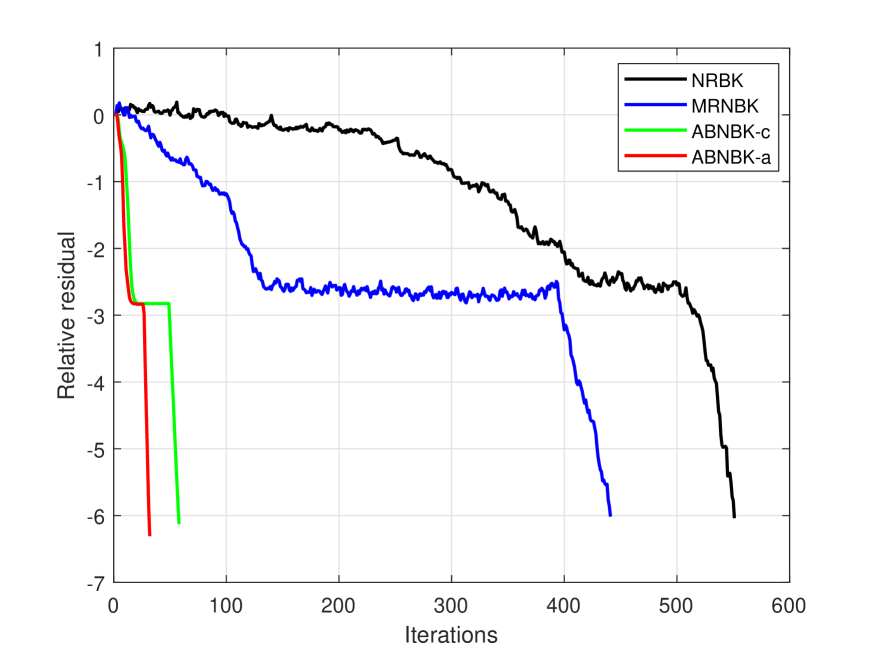
(a) $(m,n)=(200,100)$

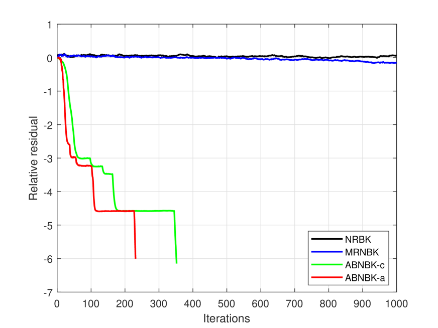
(b) $(m,n)=(1000,500)$

Figure 1: Convergence curves for Example 4.1 with $sp=0.1$.

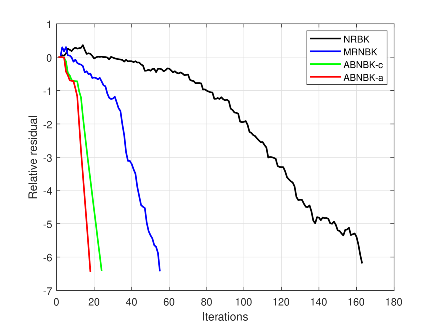
(a) $(m,n)=(200,100)$

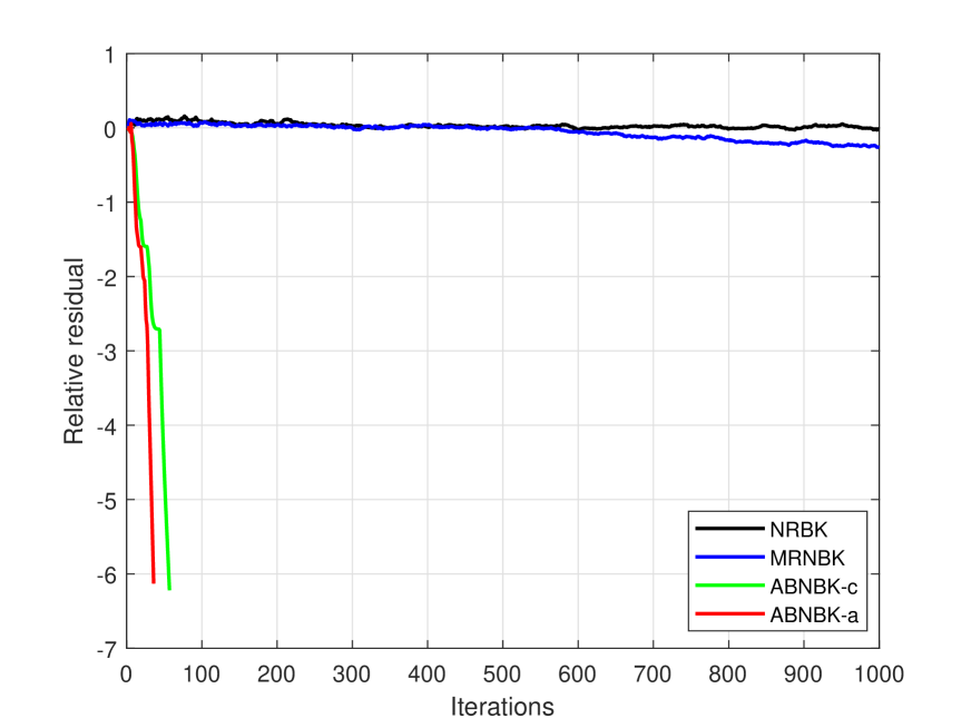
(b) $(m,n)=(1000,500)$

Figure 2: Convergence curves for Example 4.1 with $sp=0.05$.

In Figures 3 and 4, the original signal and the recovered signals by all methods when $n=500$, $sp=0.1$ and $sp=0.05$ are depicted, respectively.

From Figures 3 and 4, it is observed that the recovered signals by the ABNBK-c and ABNBK-a method are more close to the original signal than other two methods.

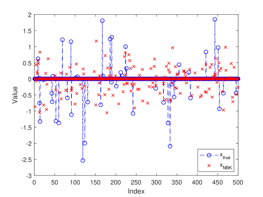
(a) NBK

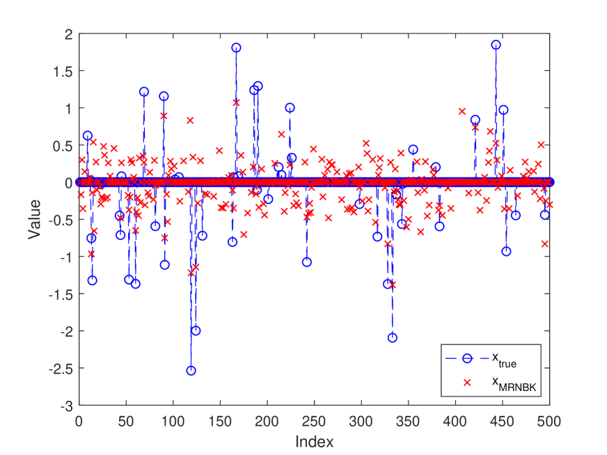
(b) MRNBK

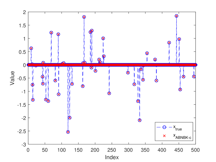
(c) ABNBK-c

(d) ABNBK-a

Figure 3: The exact signal and recovered signals for Example 4.1 with $sp=0.1$.

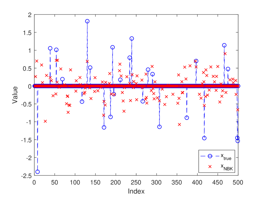
(a) NBK

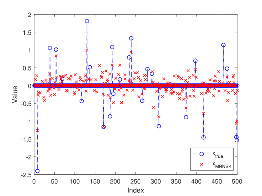
(b) MRNBK

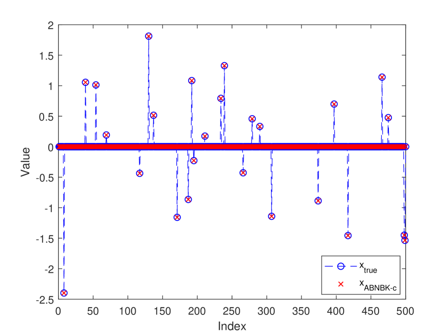
(c) ABNBK-c

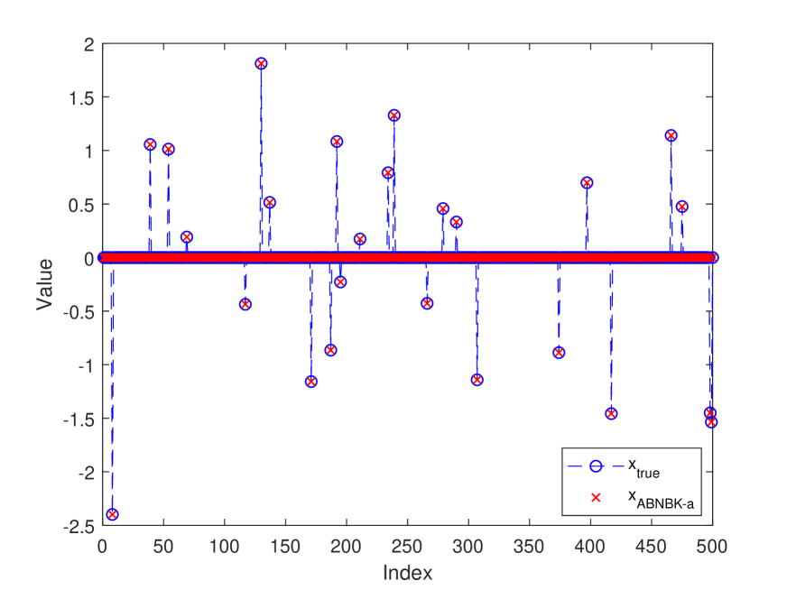
(d) ABNBK-a

Figure 4: The exact signal and recovered signals for Example 4.1 with $sp=0.05$.

Example 4.2.

In this experiment, each tested matrix $A^{(i)}(i=1,\cdots,m)$ is a random partial discrete cosine transform (DCT) matrix which $j$-th column is generated through the expression

$$A^{(i)}(:,j)=cos(2\pi(j-1)\xi),\quad j=1,\cdots,n,$$

where $\xi\in\mathbb{R}^{m\times 1}$ is a column vector with uniformly and independently sampled elements from $[0,1]$.

In Tables 3 and 4, the number of iteration steps and the elapsed CPU time for all methods when the size of $A$ and the value of $sp$ varies are listed, respectively.

From Tables 3 and 4, it is observed that the ABNBK-a method requires the fewest iteration steps and least CPU time among all methods. Moreover, the nonlinear Bregman-Kaczmarz and the maximum residual Bregman-Kaczmarz method are difficult to recover the signal as the size of the problem increases. While the proposed ABNBK method can successfully reconstruct the sparse signal within the finite iteration steps, which indicates that the ABNBK methods are advantageous for solving large nonlinear problems.

Table 3: Numerical results for Example 4.2 with $sp=0.1$.

$m$	$n$	$sp$	NBK		MRNBK		ABNBK-c		ABNBK-a
			IT	CPU	IT	CPU	IT	CPU	IT	CPU
200	100	0.1	683	18.139	926	24.716	67	2.054	35	1.083
300	150	0.1	1000	64.848	1000	65.715	381	29.113	202	14.792
400	200	0.1	1000	139.383	1000	144.561	610	98.694	403	66.817
500	250	0.1	1000	249.151	1000	257.723	774	218.658	498	148.628
600	300	0.1	1000	415.380	1000	400.643	616	264.427	167	75.847
800	400	0.1	1000	1342.724	1000	1359.726	537	819.644	254	387.752
900	450	0.1	1000	2019.286	1000	3370.743	189	431.184	123	278.255
1000	500	0.1	1000	2555.362	1000	2618.649	137	399.672	82	246.498

Table 4: Numerical results for Example 4.2 with $sp=0.05$.

$m$	$n$	sp	NBK		MRNBK		ABNBK-c		ABNBK-a
			IT	CPU	IT	CPU	IT	CPU	IT	CPU
200	100	0.05	845	24.829	332	9.351	319	10.653	229	7.491
300	150	0.05	274	18.756	159	10.888	25	1.991	16	1.280
400	200	0.05	799	112.075	868	127.403	174	27.518	103	17.404
500	250	0.05	590	142.966	315	80.687	32	9.434	21	6.125
600	300	0.05	1000	409.482	1000	423.836	51	22.340	29	13.263
800	400	0.05	1000	1348.747	676	900.045	67	105.745	41	63.521
900	450	0.05	1000	1970.914	1000	1974.391	73	164.428	42	93.813
1000	500	0.05	1000	2422.198	1000	2409.087	55	148.657	27	72.452

In Figures 5 and 6, the curves of the norm of the relative residual versus the number of iteration steps and the solution error versus the number of iteration steps for all tested methods are shown, respectively.

From Figures 5 and 6, it is seen that the ABNBK-c and ABNBK-a method converge much faster than the NBK and MRNBK methods, which shows the efficiency of the averaging technique.

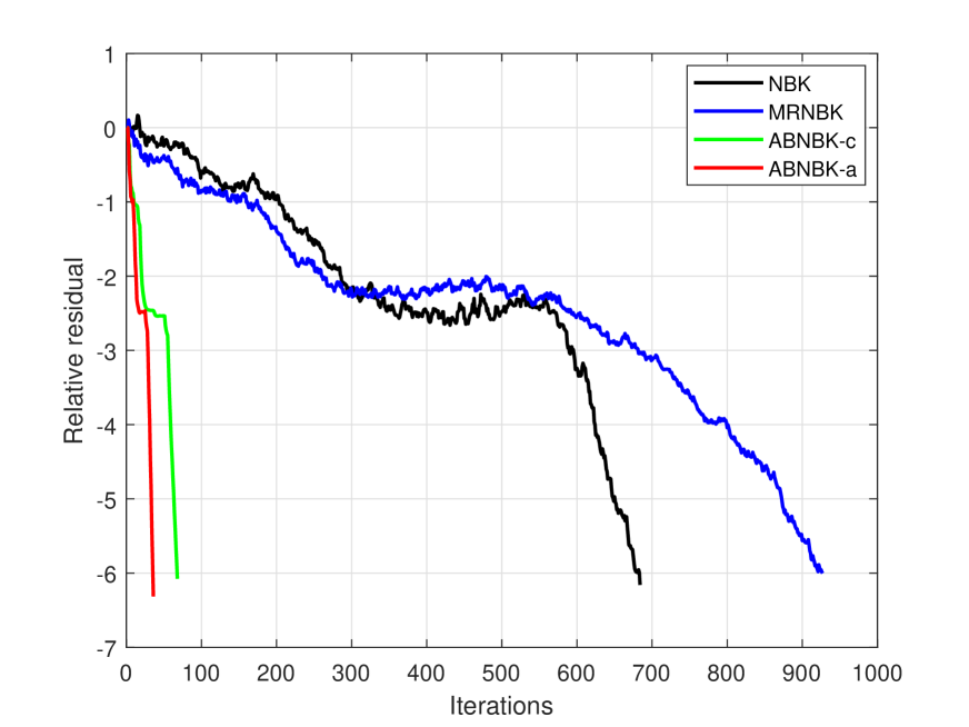
(a) $(m,n)=(200,100)$

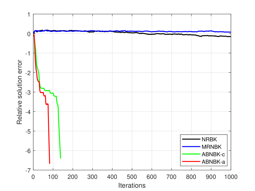
(b) $(m,n)=(1000,500)$

Figure 5: Convergence curves for Example 4.2 with $sp=0.1$.

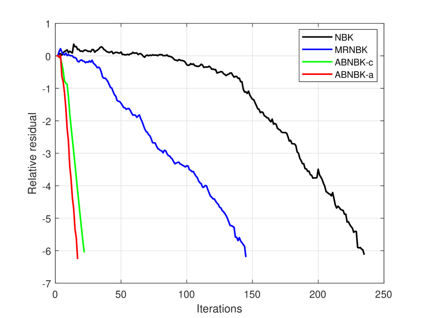
(a) $(m,n)=(200,100)$

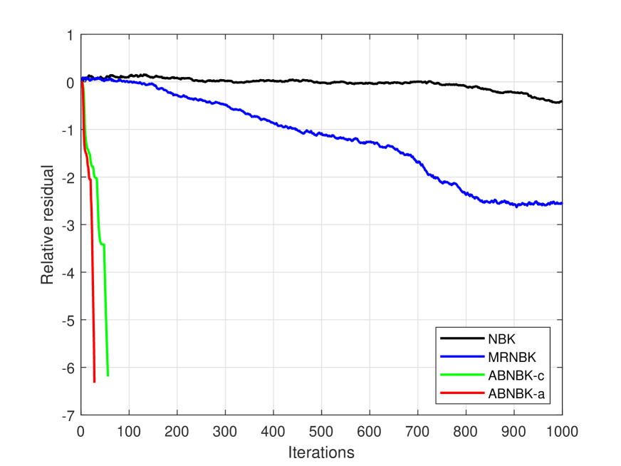
(b) $(m,n)=(1000,500)$

Figure 6: Convergence curves for Example 4.2 with $sp=0.05$.

In Figures 7 and 8, the original signal and the recovered signals by all methods when $n=500$, $sp=0.1$ and $sp=0.05$ are displayed, respectively.

From Figures 7 and 8, it is observed that the recovered signals by the ABNBK-c and ABNBK-a method are more close to the original signal than other two methods.

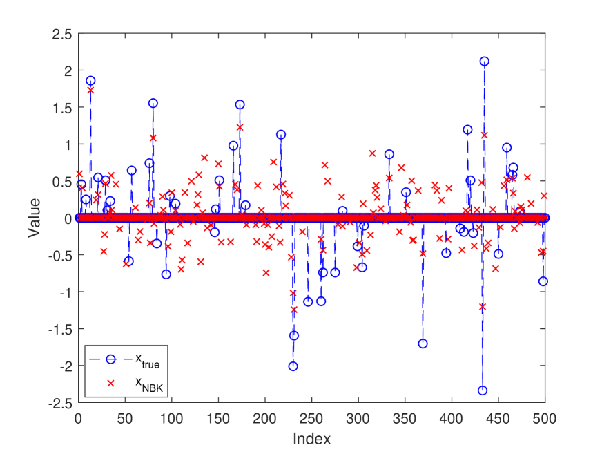
(a) NBK

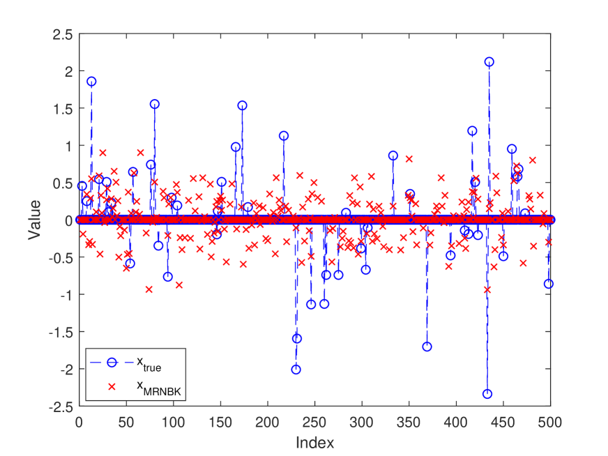
(b) MRNBK

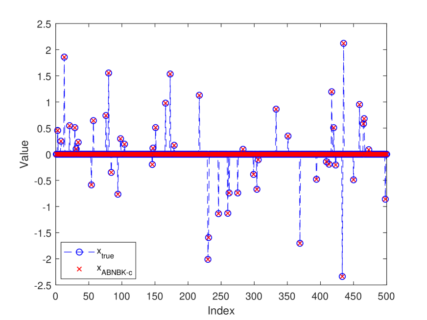
(c) ABNBK-c

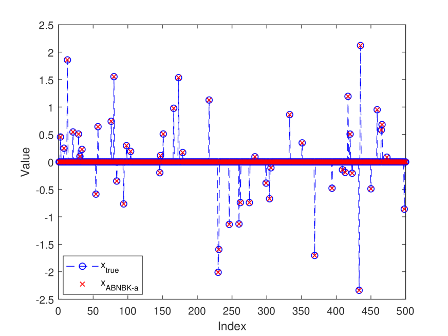
(d) ABNBK-a

Figure 7: The exact signal and recovered signals for Example 4.2 with $sp=0.1$.

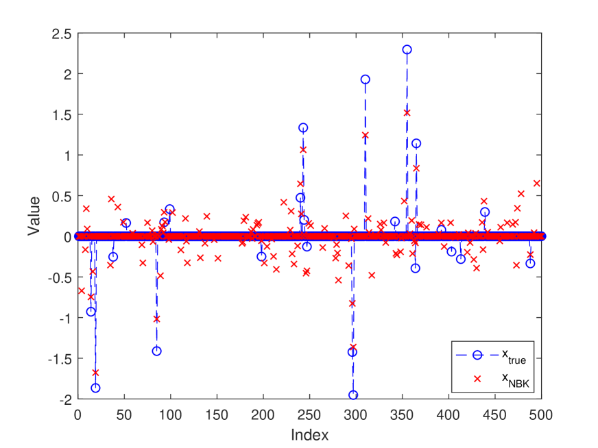
(a) NBK

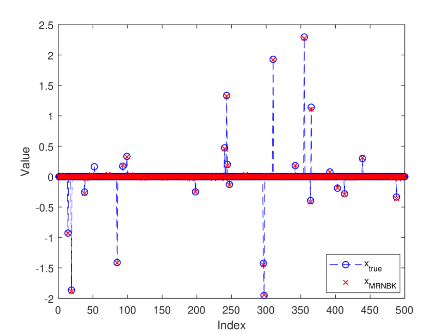
(b) MRNBK

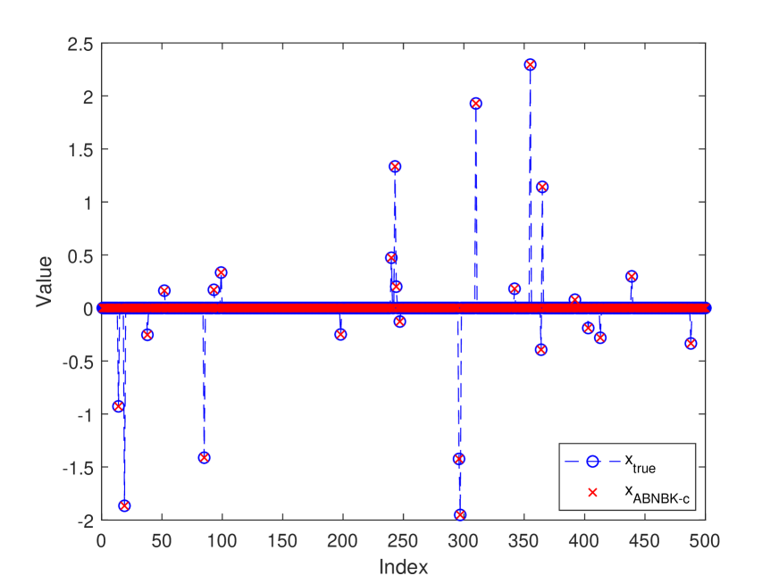
(c) ABNBK-c

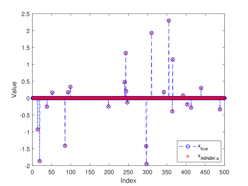
(d) ABNBK-a

Figure 8: The exact signal and recovered signals for Example 4.2 with $sp=0.05$.

5 Conclusions

In this paper, an averaging block nonlinear Bregman-Kaczmarz method is developed for the nonlinear sparse signal recovery problem. The convergence theory of the averaging block nonlinear Bregman-Kaczmarz method is established under the classical local tangential cone conditions. Moreover, the upper bound of the convergence rate of the averaging block nonlinear Bregman-Kaczmarz method with both constant stepsizes and adaptive stepsizes is given, respectively. Numerical experiments demonstrate the efficiency and robustness of the proposed method, which has faster convergence speed and fewer computing time than existing nonlinear Bregman-Kaczmarz methods.

Funding This work was supported by National Natural Science Foundation of China (No. 12471357).

References

- [1] Raman Arora, Maya R Gupta, Amol Kapila, and Maryam Fazel. Similarity-based Clustering by Left-Stochastic Matrix Factorization. Journal of Machine Learning Research, 14(7):1715–1746, 2013.
- [2] Zhongzhi Bai and Wenting Wu. On greedy randomized Kaczmarz method for solving large sparse linear systems. SIAM Journal on Scientific Computing, 40(1):A592–A606, 2018.
- [3] Amir Beck and Yonina C Eldar. Sparse signal recovery from nonlinear measurements. IEEE International Conference on Acoustics, Speech and Signal Processing, pages 5464–5468, 2013.
- [4] Thomas Blumensath. Compressed sensing with nonlinear observations and related nonlinear optimization problems. IEEE Transactions on Information Theory, 59(6):3466–3474, 2013.
- [5] Yair Censor, Dan Gordon, and Rachel Gordon. Component averaging: An efficient iterative parallel algorithm for large and sparse unstructured problems. Parallel computing, 27(6):777–808, 2001.
- [6] Kui Du, Wutao Si, and Xiaohui Sun. Randomized extended average block Kaczmarz for solving least squares. SIAM Journal on Scientific Computing, 42(6):A3541–A3559, 2020.
- [7] Guangyu Gao, Bo Han, and Shanshan Tong. A projective two-point gradient Kaczmarz iteration for nonlinear ill-posed problems. Inverse Problems, 37(7):075007, 2021.
- [8] Yu Gao and Chong Chen. Convergence Analysis of Nonlinear Kaczmarz Method for Systems of Nonlinear Equations with Component-wise Convex Mapping. arXiv preprint arXiv:2309.15003, 2023.
- [9] Yi Gong, Lin Zhang, Renping Liu, Keping Yu, and Gautam Srivastava. Nonlinear MIMO for industrial Internet of Things in cyber–physical systems. IEEE Transactions on Industrial Informatics, 17(8):5533–5541, 2020.
- [10] Robert Gower, Dirk A Lorenz, and Maximilian Winkler. A Bregman–Kaczmarz method for nonlinear systems of equations. Computational Optimization and Applications, 87(3):1059–1098, 2024.
- [11] Hengtao He, Chaokai Wen, and Shi Jin. Generalized expectation consistent signal recovery for nonlinear measurements. IEEE International Symposium on Information Theory, pages 2333–2337, 2017.
- [12] Qinian Jin and Wei Wang. Landweber iteration of Kaczmarz type with general non-smooth convex penalty functionals. Inverse Problems, 29(8):085011, 2013.
- [13] Ulugbek S Kamilov, Hassan Mansour, and Brendt Wohlberg. A plug-and-play priors approach for solving nonlinear imaging inverse problems. IEEE Signal Processing Letters, 24(12):1872–1876, 2017.
- [14] Damiana Lazzaro, Serena Morigi, and Luca Ratti. Oracle-Net for nonlinear compressed sensing in Electrical Impedance Tomography reconstruction problems. Journal of Scientific Computing, 101(2):49, 2024.
- [15] Xiaodong Li and Vladislav Voroninski. Sparse signal recovery from quadratic measurements via convex programming. SIAM Journal on Mathematical Analysis, 45(5):3019–3033, 2013.
- [16] Xiangru Lian, Wei Zhang, Ce Zhang, and Ji Liu. Asynchronous decentralized parallel stochastic gradient descent. International Conference on Machine Learning, pages 3043–3052, 2018.
- [17] Chaoyue Liu, Libin Zhu, and Mikhail Belkin. Loss landscapes and optimization in over-parameterized non-linear systems and neural networks. Applied and Computational Harmonic Analysis, 59:85–116, 2022.
- [18] Ion Necoara. Random coordinate descent algorithms for multi-agent convex optimization over networks. IEEE Transactions on Automatic Control, 58(8):2001–2012, 2013.
- [19] Ion Necoara. Faster randomized block Kaczmarz algorithms. SIAM Journal on Matrix Analysis and Applications, 40(4):1425–1452, 2019.
- [20] Ion Necoara, Peter Richtárik, and Andrei Patrascu. Randomized projection methods for convex feasibility: Conditioning and convergence rates. SIAM Journal on Optimization, 29(4):2814–2852, 2019.
- [21] Yuqi Niu and Bing Zheng. A greedy block Kaczmarz algorithm for solving large-scale linear systems. Applied Mathematics Letters, 104:106294, 2020.
- [22] Frank Schöpfer and Dirk A Lorenz. Linear convergence of the randomized sparse Kaczmarz method. Mathematical Programming, 173:509–536, 2019.
- [23] Ohad Shamir and Tong Zhang. Stochastic gradient descent for non-smooth optimization: Convergence results and optimal averaging schemes. International conference on machine learning, pages 71–79, 2013.
- [24] Chaobing Song and Jelena Diakonikolas. Cyclic coordinate dual averaging with extrapolation. SIAM Journal on Optimization, 33(4):2935–2961, 2023.
- [25] Lionel Tondji and Dirk A Lorenz. Faster randomized block sparse Kaczmarz by averaging. Numerical Algorithms, 93(4):1417–1451, 2023.
- [26] Qifeng Wang, Weiguo Li, Wendi Bao, and Xingqi Gao. Nonlinear Kaczmarz algorithms and their convergence. Journal of Computational and Applied Mathematics, 399:113720, 2022.
- [27] Aqin Xiao and Junfeng Yin. On averaging block Kaczmarz methods for solving nonlinear systems of equations. Journal of Computational and Applied Mathematics, 451:116041, 2024.
- [28] Aqin Xiao, Junfeng Yin, and Ning Zheng. On fast greedy block Kaczmarz methods for solving large consistent linear systems. Computational and Applied Mathematics, 42(3):119, 2023.
- [29] Yuxin Ye and Junfeng Yin. A residual-based weighted nonlinear Kaczmarz method for solving nonlinear systems of equations. Computational and Applied Mathematics, 43(5):276, 2024.
- [30] Rui Yuan, Alessandro Lazaric, and Robert M Gower. Sketched Newton–Raphson. SIAM Journal on Optimization, 32(3):1555–1583, 2022.
- [31] Feiyu Zhang, Wendi Bao, Weiguo Li, and Qin Wang. On sampling Kaczmarz–Motzkin methods for solving large-scale nonlinear systems. Computational and Applied Mathematics, 42(3):126, 2023.
- [32] Jianhua Zhang, Yuqing Wang, and Zhaojing. On maximum residual nonlinear Kaczmarz -type algorithms for large nonlinear systems of equations. Journal of Computational and Applied Mathematics, 425:115065, 2023.
- [33] Yanjun Zhang, Hanyu Li, and Ling Tang. Greedy randomized sampling nonlinear Kaczmarz methods. Calcolo, 61(2):25, 2024.