Enhanced Probabilistic Collision Detection for Motion Planning Under Sensing Uncertainty

Abstract

Probabilistic collision detection (PCD) is essential in motion planning for robots operating in unstructured environments, where considering sensing uncertainty helps prevent damage. Existing PCD methods mainly used simplified geometric models and addressed only position estimation errors. This paper presents an enhanced PCD method with two key advancements: (a) using superquadrics for more accurate shape approximation and (b) accounting for both position and orientation estimation errors to improve robustness under sensing uncertainty. Our method first computes an enlarged surface for each object that encapsulates its observed rotated copies, thereby addressing the orientation estimation errors. Then, the collision probability under the position estimation errors is formulated as a chance-constraint problem that is solved with a tight upper bound. Both the two steps leverage the recently developed normal parameterization of superquadric surfaces. Results show that our PCD method is twice as close to the Monte-Carlo sampled baseline as the best existing PCD method and reduces path length by $30\%$ and planning time by $37\%$, respectively. A Real2Sim pipeline further validates the importance of considering orientation estimation errors, showing that the collision probability of executing the planned path in simulation is only $2\%$, compared to $9\%$ and $29\%$ when considering only position estimation errors or none at all.

I Introduction

Collision detection is essential to motion planning, which helps to prevent robots from colliding with their surroundings. Although traditional collision detection methods have been developed for decades, they usually assume perfect knowledge of the states of robots and environments [1]. This assumption does not apply in most real-world applications, especially for service robots with a high degree of freedom (DOF) manipulating objects in domestic settings. In such cases, robots will need to interact with objects closely, but the pose estimation of objects is often affected by occlusions and sensor inaccuracies. The sensing uncertainty may cause unexpected collisions that lead to a failure of manipulation and damage the robot and the surroundings.

Compared with deterministic collision detection, probabilistic collision detection (PCD) takes into account the sensing uncertainty and calculates the collision probability between two bodies in a single query. When a PCD is used as the collision checker in a motion planner for a robot, it gives the collision probability between each link of the robot and each environmental object. PCD outcome enables the motion planner to quantify the level of safety, ensuring that the overall collision probability between the robot and objects along the planned path is lower than a given threshold.

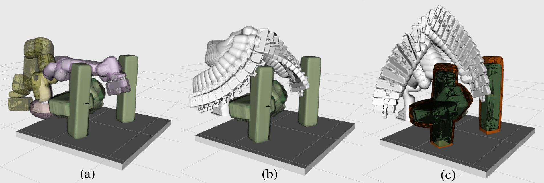
Figure 1: Comparison of motion planning results without and with considering sensing uncertainty. (a) and (c) illustrate four objects with real-world pose estimates, where each object is represented by a superquadric at the mean pose (solid green). The rotated copies of each object are shown in transparent green, encapsulated by an enlarged surface (orange). Each link of the robot arm is bounded by a superquadric. (b) shows a planned path ignoring sensing uncertainty, leading to an unexpected collision. (c) presents a more reliable path generated using the proposed PCD method, which incorporates both position and orientation estimation errors for improved safety.

However, existing PCD methods usually use a simplified geometric model (e. g., points or ellipsoids) for the robot and environmental objects and only account for position estimation errors [2, 3, 4, 5]. These assumptions may lead to less robustness when complex environmental objects cannot be accurately represented by simple geometries and when their orientation estimation errors cannot be ignored.

To address these limitations, this paper presents an enhanced PCD method with two key advancements. First, it supports using a broad class of geometric models, specifically superquadrics, to accurately approximate the true shape of environmental objects. Superquadrics are a family of geometric shapes defined by five parameters resembling ellipsoids and other quadrics. This flexibility allows them to accurately approximate the standard collision geometric models (e. g., bounding box or cylinder) or represent details of complex objects [6]. Second, the proposed method accounts for objects’ position and orientation estimation errors, increasing robustness against sensing uncertainty. Overall, these improvements enhance the reliability of PCD in unstructured environments.

We conducted a benchmark on PCD methods and found that our method considerably refines the accuracy of collision probability estimation. Besides, we examined how the accuracy and computation time of PCD methods influence the performance of motion planners. Results show that with our PCD method, planners find more efficient paths within less planning time, especially in cluttered scenes. Furthermore, we designed a Real2Sim experiment to assess the importance of considering the orientation estimation errors of objects. By comparing the collision probability of the planned paths with PCD-pose, PCD-position, and deterministic collision detection methods executed in simulation, paths generated using PCD-pose consistently exhibited the lowest risk.

The major contributions of this work are:

• Robust PCD Method: A novel method that accounts for both position and orientation uncertainties and gives a robust approximation for the collision probability.

• Hierarchical Approach: A hierarchical PCD approach that combines a fast screening method and a high-precision method to balance the computational time and accuracy.

• Real2Sim pipeline: A new pipeline that quantifies the reliability of planned paths by simulating their execution under real-world sensing uncertainties.

II Related Work

In previous works, PCD has been developed to account for uncertainties in robot controllers and environment sensing to ensure the safety of robots operating in the real world, such as drones and automatic cars [2, 7]. However, PCD for high-DOF robots is particularly challenging as they often need to interact closely with objects in cluttered scenes, such as during pick-and-place tasks. Although these robots typically operate at slower speeds, the complexity of cluttered and unstructured environments amplifies the impact of sensing uncertainty. The spatial information of the environmental objects is retrieved by noisy sensors and usually from a few partial views [8, 9].

Early PCD methods, such as Monte Carlo-based approaches, compute the collision probability accurately but are computationally demanding, limiting their practical use in real-time applications [10]. Some PCD methods that have closed-form solutions are fast to compute and are suitable for high-speed robots [11, 12, 2]. Nevertheless, they only support using simple geometrics (e. g., points, spheres, or ellipsoids) to represent robots and environmental objects, which can give a conservative result if the objects cannot be accurately represented. Besides, they only consider the position estimation errors of objects. Although some PCD methods support convex complex geometric models (e. g., mesh), their performance either depends on the surface complexity of the model [5] or needs to be iteratively improved [7]. Nevertheless, they only support the position estimation errors of objects. The learning-based method uses the point cloud of the environment and does not assume the probabilistic model per object, but the computation time is too expansive and needs to be trained for new robots [13].

Despite these advancements, current PCD methods still face limitations in accurately modeling complex shapes and handling combined position and orientation uncertainties. This work addresses these gaps by introducing a robust PCD method that leverages superquadrics for improved shape approximation and integrates position and orientation uncertainties for enhanced robustness in real-world applications.

III Preliminary

III-A Probabilistic collision detection

The collision detection problem for two convex bodies $S_{1}$, $S_{2}$ with exact poses can be solved based on the collision condition that

$$\text{if}\,S_{1}\cap S_{2}\neq\varnothing\Rightarrow\mathbf{0}\in S_{1}\oplus(-S_{2})\,.$$

where $S_{1}\oplus(-S_{2})$ is the Minkowski sum and $-S_{2}$ is the reflection of $S_{2}$ about the origin of its body frame.

If $S_{i}$ is moved by $g_{i}=(R_{i},{\bf x}_{i})\in\text{SE}(3)$, we denote the resulting body as $S_{i}^{g_{i}}=R_{i}S_{i}+x_{i}$. If the poses $g_{1}$ and $g_{2}$ are inaccurate, the collision status is probabilistic and can be written as $\text{P}(S_{1}^{g_{1}},S_{2}^{g_{2}})=P(S_{1}^{g_{1}}\cap S_{2}^{g_{2}}\neq\varnothing)$.

III-B Collision probability under position estimation uncertainty

Previous PCD methods only consider the positions of objects to be inaccurate, in which case $g_{i}=(\mathbb{I}_{3},{\bf x}_{i})$. The inaccurate point set is then $S_{i}^{g_{i}}=S_{i}+{\bf x}_{i}$. In this case, the collision condition becomes:

$$\left(S_{1}+{\bf x}_{1}\right)\cap\left(S_{2}+{\bf x}_{2}\right)\neq\varnothing\Rightarrow({\bf x}_{2}-{\bf x}_{1})\in S_{1}\oplus(-S_{2})\,.$$

The collision probability can be written as an integral for:

$$\text{P}(S_{1}^{g_{1}},S_{2}^{g_{2}})$$ (1)

$$=\thinspace\int_{\mathbb{R}^{3}}\thinspace\int_{\mathbb{R}^{3}}\thinspace\iota({\bf x}_{2}-{\bf x}_{1}\in S_{1}\oplus(-S_{2}))\rho_{1}({\bf x}_{1})\rho_{2}({\bf x}_{2})d{\bf x}_{1}d{\bf x}_{2}\,,$$

where $\iota(\cdot)$ is an indicator function that equals $1$ if the inner condition is true and $0$ otherwise. $\rho(\cdot)$ is the shorthand for the probability density function (pdf) defined by the argument.

The position error is usually modeled as Gaussian distributed because its source is from many factors, like noisy sensors and partial occlusion, based on the central limit theorem. If the position errors ${\bf x}_{1}$ and ${\bf x}_{2}$ of the objects are independent, the relative position error ${\bf x}={\bf x}_{2}-{\bf x}_{1}$ is also Gaussian distributed. However, this integration has no closed-form solution, and its numerical solution is computationally expensive.

III-C Linear chance constraint approximation

Eq. LABEL:eq:pre:pcd-position is usually written as a chance-constraint problem $\text{P}(S_{1}^{g_{1}},S_{2}^{g_{2}})\leq\delta$, where $\delta$ is an upper bound for the collision probability. When ${\bf x}$ is Gaussian distributed (i.e., ${\bf x}\sim\mathcal{N}({\bf p}_{x},\Sigma_{x})$, $\delta$ has a closed-form solution [14].

The idea is that the integration of a Gaussian distributed variable ${\bf x}$ inside a linear half-space can be transformed as a cumulative distribution function (cdf) of a new 1D Gaussian variable [14]:

$$\int_{\mathbf{a}^{T}{\bf x}-b<0}\rho({\bf x};{\bf p}_{x},\Sigma_{x})d{\bf x}=\int_{y<0}\rho(y;p_{y},\sigma_{y})d{\bf x}\,,$$

where $\mathbf{a}^{T}{\bf x}-b<0$ defines a linear half-space with the normal $\mathbf{a}$ and the constant $b$, and $y=\mathbf{a}^{T}{\bf x}-b$ is a 1D variable that follows Gaussian distribution $\mathcal{N}(\mathbf{a}^{T}{\bf p}_{x}-b,\mathbf{a}^{T}\Sigma_{x}\mathbf{a})$. The cdf result $F_{y}(0)$ can be easily found by the look-up table.

This means that if the integration region $S_{1}\oplus(-S_{2})$ in Eq. LABEL:eq:pre:pcd-position is fully contained by a linear half-space, the collision probability in Eq. LABEL:eq:pre:pcd-position can be bounded by

$$\text{P}(S_{1}^{g_{1}},S_{2}^{g_{2}})=\int_{S_{1}\oplus(-S_{2})}\rho({\bf x};{\bf p}_{x},\Sigma_{x})d{\bf x}<F_{y}(0)\,.$$ (2)

The accuracy of the approximation depends on the choice of the linear half-space. Previous methods choose a naive plane with a closed-form solution by using the normalized ${\bf p}_{x}$ as the normal $\mathbf{a}$ when objects are spheres or ellipsoids [2, 3]. This method is named as lcc-center for reference.

Although lcc-center is computationally efficient, the geometric models are limited, and the result using such a plane can be conservative. In this work, we propose a linear half-space that gives a more accurate approximation for the collision probability than lcc-center.

III-D Normal-parameterized surface

The implicit function of the surface of a superquadric is given as:

$$\Psi({\bf x})=\left(\left(\frac{x_{1}}{a_{1}}\right)^{\frac{2}{\epsilon_{2}}}+\left(\frac{x_{2}}{a_{2}}\right)^{\frac{2}{\epsilon_{2}}}\right)^{\frac{\epsilon_{2}}{\epsilon_{1}}}+\left(\frac{x_{3}}{a_{3}}\right)^{\frac{2}{\epsilon_{1}}}-1=0\,,$$

where $\epsilon_{1}\,,\epsilon_{2}\in(0,2)$ to ensure the convexity. When $\epsilon_{1}=\epsilon_{2}=1$, superquadrics become ellipsoids. When $\epsilon_{1}=\epsilon_{2}=0.2$, superquadrics are approximations for cuboids. Besides the implicit function, the surface has a spherical parameterization ${\bf x}=\mathbf{f(\boldsymbol{\psi})}$, where $\boldsymbol{\psi}\in\mathbb{R}^{N-1}$ for body $S$ in $\mathbb{R}^{N}$ [1].

With the implicit expression of superquadrics, the gradient ${\bf m}$ is given as ${\bf m}({\bf x})=\nabla_{\bf x}\Psi({\bf x})$ and the normal ${\bf n}({\bf x})$ is the normalized ${\bf m}({\bf x})$. Because the surface of superquadrics is limited to be convex, smooth, and positively curved, the mapping between the surface points ${\bf x}$ and their normal ${\bf n}$ exists and is unique. The inverse mapping ${\bf x}={\bf x}({\bf n})$ of ${\bf n}={\bf n}({\bf x})$ can also be found [1].

Because $S_{1}$ and $S_{2}$ are convex, the contact point between them is a single point, and the surface normals of the two bodies at the contact point are anti-parallel. Thus, the point on the Minkowski sum boundary ${\bf x}_{\Sigma}\in\partial[S_{1}\oplus(-S_{2})]$ can be parameterized by its normal: ${\bf x}_{\Sigma}({\bf n})={\bf x}_{1}({\bf n})-{\bf x}_{2}(-{\bf n})$, where $\partial(\cdot)$ represents the boundary of a body, and ${\bf n}$ is the normal of $\partial[S_{1}\oplus(-S_{2})]$ and $\partial S_{1}$.

If applying the rotations $R_{1},R_{2}\in SO(3)$ to objects, ${\bf x}_{\Sigma}\in\partial[R_{1}S_{1}\oplus(-R_{2}S_{2})]$ can be written as ${\bf x}_{\Sigma}({\bf n})=R_{1}{\bf x}_{1}(R_{1}^{T}{\bf n})-R_{2}{\bf x}_{2}(-R_{2}^{T}{\bf n})$, where ${\bf n}$ is the normal of $\partial[R_{1}S_{1}\oplus(-R_{2}S_{2})]$, $R_{1}^{T}{\bf n}$ and $R_{2}^{T}{\bf n}$ is the normal of the original body boundary $\partial S_{1}$ and $\partial S_{1}$, respectively.

IV Probabilistic Collision Detection

This section first introduces the properties of the pose estimation errors. Next, the collision probability under the pose estimation errors is formulated. Then, the method to handle the orientation errors is proposed. After that, the linear chance constraint approximation for the collision probability under position errors using the optimization is introduced and is named lcc-tangent. Moreover, the hierarchical PCD method, h-lcc, is proposed to balance the computational time and accuracy.

IV-A Properties of pose estimation errors

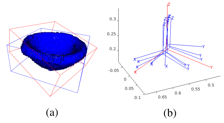
Figure 2: Demonstration of the pose estimates for an object. (a) A pose estimates for a bowl from real-world perception. (b) Several pose estimates for the bowl in the same scene.

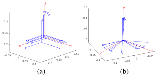
Figure 3: The position estimation (a) and orientation estimation (b) of a bowl. The mean position and mean orientation are shown in red coordinates. The translated and rotated copies are shown in blue coordinates.

An example of pose estimates for a bowl from the real world is shown in Fig. 2 (a). In this work, we treat the position and orientation estimates as independent. The $m$ position and orientation estimates for the body $S_{i}$ are denoted as $\{{\bf x}_{ij}\}$ and $\{R_{ij}\}$, where $j=[1,\cdots,m]$. For the position estimation errors, it is assumed to be Gaussian distributed, i.e., ${\bf x}_{i}\sim\mathcal{N}({\bf p}_{i},\Sigma_{i})$. The mean position ${\bf p}_{i}$ is computed by $\sum_{j=1}^{m}({\bf p}_{ij}-{\bf p}_{i})=\mathbf{0}$ and the covariance is $\Sigma_{i}=\frac{1}{m}\sum_{j=1}^{m}({\bf p}_{ij}-{\bf p}_{i})({\bf p}_{ij}-{\bf p}_{i})^{T}$. For the orientation estimation errors, the mean orientation $R_{i}$ is defined as:

$$\sum_{j=1}^{m}\log(R_{i}^{T}R_{ij})=\mathbb{O}_{3}\,,$$

where $\log(\cdot)$ is the matrix logarithm. The mean orientation can be found by iteratively solving the above equation [15].

IV-B PCD for pose estimation errors

The collision probability under pose estimation errors can be written as:

$$\text{P}(S_{1}^{g_{1}},S_{2}^{g_{2}})\thinspace$$ (3)

$$=\thinspace\int_{SE(3)}\thinspace\int_{SE(3)}\thinspace\iota(S_{1}^{g_{1}}\cap S_{2}^{g_{2}}\neq\varnothing)\rho_{1}(g_{1})\rho_{2}(g_{2})dg_{1}dg_{2}.$$

Because we consider the position and orientation estimates as independent, the uncertainties are independent, i.e., $\rho_{i}(g_{i})=\rho_{i}({\bf x}_{i})\rho_{i}(R_{i})$.

To handle the orientation errors, we do not explicitly compute the probabilistic model $\rho_{i}(R_{i})$. Instead, we choose to expand the surface of $S_{i}$ so that the enlarged surface encapsulates its rotated copies ${R_{ij}}$, which is inspired by the geometric-based PCD method for position errors [7]. Denoted the enlarged surface of $S_{i}$ as $S_{i}^{UB}$.

Because the position estimates between $S_{1}$ and $S_{2}$ are independent, the distribution of the relative position error ${\bf x}={\bf x}_{2}-{\bf x}_{1}$ is ${\bf x}\sim\mathcal{N}({\bf p}_{x},\Sigma_{x})$, where ${\bf p}_{x}={\bf p}_{2}-{\bf p}_{1}$ and $\Sigma_{x}=\Sigma_{2}+\Sigma_{1}$.

With $S_{1}^{UB}$ and $S_{2}^{UB}$, we get the inequality of Eq. 3 as:

$$\text{P}(S_{1}^{g_{1}},S_{2}^{g_{2}})<\int_{\mathbb{R}^{3}}\iota({\bf x}\in S_{1}^{UB}\oplus(-S_{2}^{UB}))\rho({\bf x})d{\bf x}\,.$$ (4)

The goal is that the approximation of the collision probability is accurate and robust for the sensing uncertainty.

IV-C Orientation estimation errors

To find the enlarged surface of $S_{i}^{UB}$, we propose a closed-form expression of the form:

$${\bf x}_{i}^{UB}({\bf n}_{i})=\frac{c}{m}\left(\sum_{j=1}^{m}R_{ij}{\bf x}_{i}(R_{ij}^{T}{\bf n}_{i})\right)\,,$$ (5)

where ${\bf x}_{i}^{UB}({\bf n}_{i})\in\partial S_{i}^{UB}$, and ${\bf n}_{i}$ is the normal of $\partial S_{i}^{UB}$ at ${\bf x}_{i}^{UB}$. The meaning of Eq. 5 is the Minkowski sum of $m$ rotated copies of $S_{i}$ scaled down by $m$ to result in the ‘average body’ that reflects the contribution of the rotated copies, and scaled up by a constant $c$ to ensure encapsulation. In this work, we choose an empirical value of $c=1.2$. An example is shown in Fig. 4. The enlarged surface is built online in collision checking.

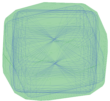
Figure 4: An enlarged surface of $S_{i}^{UB}$ that encapsulates the observed rotated copies of $S_{i}$. The boundary lines of the rotated copies are in blue and the surface of $S_{i}^{UB}$ is in green.

The Minkowski sum boundary ${\bf x}_{\Sigma}^{UB}({\bf n})\in\partial[S_{1}^{UB}\oplus(-S_{2}^{UB})]$ can be written as:

$${\bf x}_{\Sigma}^{UB}({\bf n})={\bf x}_{1}^{UB}({\bf n})-{\bf x}_{2}^{UB}(-{\bf n})$$ (6)

$$=\thinspace\frac{c}{m}\thinspace\left(\thinspace\sum_{j=1}^{m}\thinspace R_{1j}{\bf x}_{1}(R_{1j}^{T}{\bf n})\thinspace-\thinspace\sum_{j=1}^{m}\thinspace R_{2j}{\bf x}_{2}(-R_{2j}^{T}{\bf n})\right)\thinspace.$$

If one body $S_{i}$ has no orientation estimation errors, $R_{ij}$ is the mean orientation $R_{i}$.

IV-D Position estimation errors

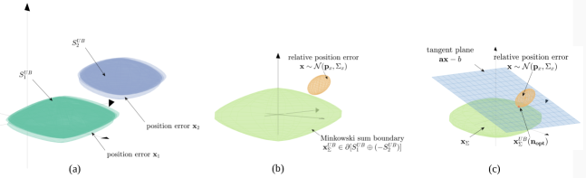
Figure 5: Illustration of the linear chance constraint method lcc-tangent. (a) The randomly generated superquadrics $S_{1}^{UB}$ and $S_{2}^{UB}$, and the effect of the position errors ${\bf x}_{1}$ and ${\bf x}_{2}$; (b) the Minkowski sum boundary points ${\bf x}_{\Sigma}^{UB}({\bf n})\in\partial[S_{1}^{UB}\oplus(-S_{2}^{UB})]$, and the ellipsoidal level surface of the relative position error ${\bf x}={\bf x}_{2}-{\bf x}_{1}$; (c) the transformed Minkowski sum boundary points ${\bf x}_{\Sigma}^{UB^{\prime}}$ and transformed relative position error center ${\bf p}_{x}^{\prime}$; (d) the final tangent half-space in the untransformed space based on Eq. 8.

After finding the $S_{i}^{UB}$, the PCD problem is to solve Eq. 4. We choose to solve Eq. 4 as a chance-constraint problem:

$$\int_{\mathbb{R}^{3}}\iota({\bf x}\in S_{1}^{UB}\oplus(-S_{2}^{UB}))\rho({\bf x})d{\bf x}<\delta\,,$$ (7)

where $\delta$ is an upper bound and can be solved in closed form. As shown in Eq. 2, the accuracy of the upper bound $\delta$ for $\text{P}(S_{1}^{g_{1}},S_{2}^{g_{2}})$ depends on the choice of the linear half-space. For a Gaussian-distributed position error ${\bf x}$, the confidence level surface is an ellipsoid, with higher pdf values closer to the center. If the chosen plane is tangent to both the Minkowski sum boundary and the confidence level surface, the resulting half-space contains less of the high pdf region. This provides a better linearization for the chance-constrained PCD problem than the previous lcc-center.

To find the tangent half-space, it is important to make the plane tangents to the confidence level surfaces. Because a confidence level surface is an ellipsoid, as shown in the orange curves in Fig. 5(b). An easy way to find its tangent plane is to transform the ellipsoid into a sphere. This is done by applying the linear transformation $\Sigma_{x}^{-1/2}$ to the whole space. The transformed position error distribution becomes ${\bf x}^{\prime}\sim\mathcal{N}({\bf p}_{x}^{\prime},\mathbb{I})$, where ${\bf p}_{x}^{\prime}=\Sigma_{x}^{-1/2}{\bf p}_{x}$. Given two enlarged superquadircs, their Minkowski sum region ${\bf x}_{\Sigma}^{UB}$ before the linear transformation is shown in the green region in Fig. 5(b). ${\bf x}_{\Sigma}^{UB}$ after the transformation can be calculated as ${\bf x}_{\Sigma}^{UB^{\prime}}=\Sigma_{x}^{-1/2}{\bf x}_{\Sigma}^{UB}$, which still has the closed-form solution and remains to be convex. Fig. 5(c) shows a confidence level surface and ${\bf x}_{\Sigma}^{UB^{\prime}}$ in the transformed space.

The problem of finding the tangent half-space is formulated to find a tangent plane on ${\bf x}_{\Sigma}^{UB^{\prime}}({\bf n})$ with the shortest distance to the center ${\bf p}_{x}^{\prime}$. This can be formulated as a nonlinear least squares optimization:

$$\min_{\psi}\frac{1}{2}||{\bf p}_{x}^{\prime}-{\bf x}_{\Sigma}^{UB^{\prime}}({\bf n}(\boldsymbol{\psi}))||_{2}^{2}\,,$$ (8)

which is solved by the trust region algorithm.

Because the optimization in Eq. 8 is not convex, it does not guarantee the global minimal and is sensitive to the initial value $\psi_{0}$. Inspired by [1], this work uses the angular parameter of the center of the position error ${\bf p}_{x}^{\prime}$ as viewed in the body frame of $S_{1}$ with the mean rotation $R_{1}$, denoted as $\leftidx{{}^{1}}{\bf p}_{x}^{\prime}=R_{1}^{T}{\bf p}_{x}^{\prime}$. For 3D cases, $\psi_{0}$ equals to:

$$[\text{atan2}\left(\leftidx{{}^{1}}{\bf p}_{x,3}^{\prime},\sqrt{(\leftidx{{}^{1}}{\bf p}_{x,1}^{\prime})^{2}+(\leftidx{{}^{1}}{\bf p}_{x,2}^{\prime})^{2}}\right),\text{atan2}\left(\leftidx{{}^{1}}{\bf p}_{x,2}^{\prime},\leftidx{{}^{1}}{\bf p}_{x,1}^{\prime}\right)]$$

After finding the optimized value $\psi_{\text{opt}}$, the normal $\mathbf{a}$ and constant $b$ of the tangent half-space in the untransformed space are $\mathbf{a}={\bf n}_{\text{opt}}(\psi_{opt})$ and $b={\bf n}_{\text{opt}}^{T}{\bf x}_{\Sigma}^{UB}({\bf n}_{\text{opt}})$, respectively. Substituting $\mathbf{a}$ and $b$ into Eq. 2, the accurate approximation can be calculated, named as lcc-tangent for reference.

IV-E Hierarchical PCD

Although the proposed lcc-tangent gives a tight approximation for the collision probability, the existing lcc-center computes faster and can be helpful to quickly screen out low collision probability regions. Therefore, this work proposed a hierarchical PCD method, named h-lcc, to balance between computation time and better estimation.

The pseudocode of h-lcc is shown in Algorithm 1. For a pair of objects, their ellipsoids (E) and superquadrics (S) collision models are known and denoted as $E_{1}^{UB}\,,S_{1}^{UB}$ and $E_{2}^{UB}\,,S_{2}^{UB}$, respectively. Noted that $S_{i}^{UB}\subset E_{i}^{UB}$. The collision models are given as the input, together with the relative position error distribution $\mathcal{N}({\bf p}_{x},\Sigma_{x})$ and the collision threshold $\delta$. The outputs include the estimation of their exact collision probability $P$ and their collision status relative to the threshold.

Line 1 of the algorithm approximates $P(E_{1}^{UB},E_{2}^{UB})$ by using Eq. 5 to compute $E_{i}^{UB}$ and the plane with normalized ${\bf p}_{x}$ as the normal, inspired by lcc-center, to get the upper bound as in Eq. 4. If $P(E_{1}^{UB},E_{2}^{UB})<\delta$, then the output probability is $P(S_{1}^{g_{1}},S_{2}^{g_{2}})=P(E_{1}^{UB},E_{2}^{UB})$ and the algorithm terminates. If this value exceeds a predefined threshold $\delta$, a more accurate calculation $P(S_{1}^{UB},S_{2}^{UB})$ using lcc-tangent is performed in Line 1 with the tangent plane using Eq.8. And the output collision probability is $P(S_{1}^{g_{1}},S_{2}^{g_{2}})=P(S_{1}^{UB},S_{2}^{UB})$. If the refined probability still exceeds $\delta$, the Boolean variable inCollision is set to 1. Otherwise, inCollision is set to 0.

Inputs : $S_{1}^{UB},S_{2}^{UB},E_{1}^{UB},E_{2}^{UB},\mathcal{N}({\bf p}_{x},\Sigma_{x}),\delta$

Outputs : $P$, inCollision

1 Compute $P(E_{1}^{UB},E_{2}^{UB})$ using lcc-center;

2 if $P(E_{1}^{UB},E_{2}^{UB})>\delta$ then

3    Compute $P(S_{1}^{UB},S_{2}^{UB})$ using lcc-tangent;

4    $P$ = $P(S_{1}^{UB},S_{2}^{UB})$;

5    if $P(S_{1}^{UB},S_{2}^{UB})>\delta$ then

6       inCollision = $1$;

7      

8   else

9       inCollision = $0$;

10      

11    end if

12   

13else

14    $P$ = $P(E_{1}^{UB},E_{2}^{UB})$;

15    inCollision = $0$;

16   

17 end if

Algorithm 1 Hierarchical probabilistic collision checker h-lcc.

V Results

This section evaluates the performance (i.e., accuracy and computational time) of lcc-tangent, compared to existing methods. It also assesses the efficiency of lcc-tangent and h-lcc in motion planning under position estimation errors against the baseline method, lcc-center. Lastly, a Real2Sim benchmark examines the importance of accounting for pose sensing uncertainty. All benchmarks are executed on an Intel Core i9-10920X CPU at 3.5GHz.

V-A Benchmark on a single query of PCD

This benchmark compares the proposed PCD methods with state-of-the-art approaches for convex bodies under Gaussian-distributed position errors. Two shape models (ellipsoids and superquadrics) and two error scenarios (one body vs. both bodies having independent position errors) yield four test cases: ellipsoids-single-error, superquadrics-single-error, ellipsoids-two-errors, and superquadrics-two-errors.

V-A1 Benchmark setting

Each test generates 100 random object pairs. The semi-axes $[a_{1},a_{2},a_{3}]$ of a body are sampled from $(0.2,1.2)$ m. The epsilon variables $[\epsilon_{1}$, $\epsilon_{2}]$ are set to $[1,1]$ for ellipsoids and are randomly sampled in the range of $(0.01,0.2)$ for superquadrics. Object centers are sampled in $(0.0,0.1)$ m and $(0.3,1.3)$ m, respectively. The orientations are uniformly sampled in $\text{SO}(3)$. Position errors follow a Gaussian distribution with covariance $\Sigma=R\Sigma_{x}R^{T}$, where $\Sigma_{x}=[4.8,0,0;0,4.8,0;0,0,6.0]*10^{-4}$ in each object’s local frame and $R\in\text{SO}(3)$.

The PCD methods included in the benchmark are summarized in Table. I. The baseline for single-error cases employs $10^{4}$ Monte Carlo samples of translated copies of $S_{2}$ based on its position error distribution. For double-error cases, a fast Monte Carlo approach generates $10^{5}$ translated copies of object $S_{2}$ based on the relative position error distribution [10]. In both cases, the deterministic collision status of translated $S_{2}$ with $S_{1}$ is computed for each sample to estimate collision probability. EB95 is the enlarged bounding volume method with $95\%$ confidence [7]. Divergence [5] applies the divergence theorem to meshed object surfaces (100 points for ellipsoids, 1600 for superquadrics), excluding mesh construction time for fairness of comparison. lcc-center uses the linear chance constraint method [2][3]. As for applying lcc-center in superquadrics cases, we first compute the minimum volume enclosing ellipsoids for the superquadrics, and the computation time for computing the bounding ellipsoid is not counted for fairness. lcc-tangent is the proposed method of this study in Eq. 8.

TABLE I: Algorithms used in the PCD benchmark.

Notation	Method
Baseline for single error	Monte-Carlo Sampling
Baseline for two errors [10]	Fast Monte-Carlo sampling
EB95 [7]	Bounding volume with $95\%$ of confidence
Divergence [5]	Divergence theorem
lcc-center [3]	Linear chance constraint for ellipsoids
lcc-tangent (ours)	Eq. 8

V-A2 Benchmark results

If any result exceeds $1$, the value is truncated to $1$. The differences between each PCD method and the baseline for all tests are summarized in Table. II. Overall, lcc-tangent is the most accurate, closely matching the baseline with lower mean and variance. Compared to divergence, which relies on mesh discretization, lcc-tangent approximates the collision probability only using one inequality. Although EB95 can increase accuracy by raising the expansion confidence, this also increases computation time. Meanwhile, lcc-center is the fastest since it skips optimization, but it is generally less accurate than lcc-tangent, which leverages a plane tangent to both the exact Minkowski sum boundary and the position error’s confidence level surface to avoid conservativeness.

TABLE II: PCD benchmark results. The table presents the mean and variance of the differences between each PCD method and the baseline.

		Mean	Variance	Computation time(s)
	EB95	0.0511	0.0310	0.0069
ellipsoids	Divergence	0.0945	0.0651	0.0044
single error	lcc-center	0.0296	0.0096	1.7396e-4
	lcc-tangent (ours)	0.0162	0.0063	0.0090
	EB95	0.4885	0.2172	0.0093
superquadrics	Divergence	0.5072	0.2114	0.0172
single error	lcc-center	0.5634	0.1949	1.9544e-4
	lcc-tangent (ours)	0.4153	0.2099	0.0143
	EB95	0.1435	0.1014	0.0053
ellipsoids	Divergence	0.1041	0.0713	0.0040
two errors	lcc-center	0.0212	0.0055	1.4908e-04
	lcc-tangent (ours)	0.0142	0.0043	0.0097
	EB95	0.2439	0.1597	0.0128
superquadrics	Divergence	0.1334	0.1231	0.0193
two errors	lcc-center	0.2078	0.1105	2.1014e-04
	lcc-tangent (ours)	0.0226	0.0129	0.0136

V-B Benchmark on planning under position estimation errors

We evaluate how PCD computational accuracy and runtime affect motion planning, comparing lcc-center (baseline), lcc-tangent, and h-lcc used as the sub-modules in RRT-connect (sampling-based) [16] and STOMP (optimization-based) [17] planners.

V-B1 Benchmark setting

The environment settings are shown in Fig. 6. The high-precision industrial robot Franka Emika with the fixed basement is used, and the pose estimation error of the robot can be ignored. The start and goal joint configurations are pre-defined for each setting. Each link of the robot arm is bounded by an ellipsoid, and all obstacles are ellipsoids. In addition, the obstacles are only considered to have position errors, where $\Sigma=R\Sigma_{x}R^{T}$, $\Sigma_{x}=[4.8,0,0;0,4.8,0;0,0,6.0]*10^{-4}$ in the body-fixed frame, and $R\in\text{SO}(3)$ is the obstacle’s orientation. Because all obstacles are static, their position errors will not be propagated. We set the collision threshold to be $\delta=0.05$. A robot configuration is invalid if any PCD result for a link–obstacle pair exceeds $\delta$. Each environment setup is tested 100 times.

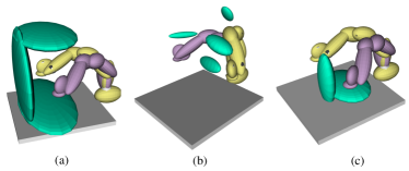
Figure 6: Three types of environments used in the planning benchmark: (a) clamp, (b) narrow, and (c) sparse. All obstacles are ellipsoids and subjected to position errors. The violet and yellow colors represent the start and goal joint configurations of the arm. Each robot link is bounded by an ellipsoid.

V-B2 Benchmark results

The average path length and planning time for the success cases are listed in Table. III, with changes shown relative to lcc-center. In all cases, the proposed PCD methods (lcc-tangent and h-lcc) produce shorter paths by avoiding overly conservative collision checks.

The observed differences in computation time between the two planners stem from their fundamentally different path-planning approaches. RRTconnect relies on random configuration exploration to find a valid path. Since the query time of lcc-tangent is longer than that of lcc-center, the overall exploration speed of RRTconnect is slower when using lcc-tangent. In contrast, STOMP’s iterative process allows it to benefit from the precise collision checking provided by lcc-tangent and h-lcc. The accuracy of these methods enables STOMP to converge faster to an optimized path, leading to reductions in both path length and planning time.

TABLE III: Planning benchmark results. The change rate is relative to the result of the baseline PCD method.

Motion planner	Environment	PCD method	Success rate	Path length (rad)	Change rate	Planning time (s)	Change rate
RRTconnect		lcc-center	1	5.24	-	1.28	-
	clamp	lcc-tangent (ours)	1	4.90	-6.78%	2.62	111.72%
		h-lcc (ours)	1	3.72	-30.19%	1.06	-14.41%
		lcc-center	1	8.24	-	5.70	-
	narrow	lcc-tangent (ours)	0.9	7.28	-11.72%	9.25	62.46%
		h-lcc (ours)	0.98	7.65	-7.15%	8.39	47.28%
STOMP		lcc-center	1	8.40	-	21.04	-
	sparse	lcc-tangent (ours)	1	7.15	-17.88%	17.44	-17.11%
		h-lcc (ours)	1	7.15	-17.88%	13.06	-37.93%

V-C Real2Sim pipeline for pose estimation errors

This benchmark is designed to test the safety of the planned path in execution when considering different types of sensing uncertainty in motion planning. Here, we create a typical manipulation setting, and the objects’ pose estimation is done in the real world. The pose estimation results are used in motion planning when considering none sensing errors (baseline), position estimation errors, and both position and orientation estimation errors. After that, we test the collision probability between the robot and objects in the simulation, where the simulation environment rolls out the possibility of the robot executing the planned path in the real world.

V-C1 Benchmark setting

The experiment setting is shown in Fig. 7 (a). A Franka Emika robot arm moves from a fixed start to a goal configuration. Each robot link is bounded by a superquadric. Object shapes are known, while their poses are sensed via RGB-D cameras: bowl and chair through iterative closest point (ICP), and boxes through ArUco markers. From each pose estimates, we extract the position error distribution and mean orientation.

We run RRTconnect with three collision checkers over 100 trials each: a deterministic checker (cfc-dist-ls [1]), a PCD method handling position errors (lcc-tangent), and a PCD method for pose errors (encapsulated surfaces + lcc-tangent).

Each set of 100 planned paths is executed four times in simulation, once for each of the four objects. At each run, the object’s pose is updated randomly from the pose estimations from real-world measurements. Paths are marked “unsafe” if any via point collides with an object, and the collision probability is the fraction of unsafe paths.

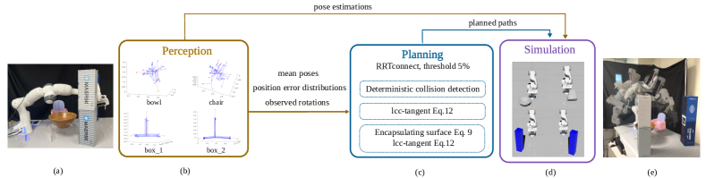
Figure 7: Real2Sim pipeline to evaluate the reliability of planned paths using different PCD methods. (a) A typical manipulation setting with four objects. (b) Perception results for each object. (c) Motion planning with different PCD methods. (d) Rolling out the possibility of the robot executing the planned path in simulation (Isaac Sim) and calculating the collision probability in execution. (e) A collision-free path in simulation is executed in the real world, which is planned under considering pose sensing uncertainty.

V-C2 Benchmark results

The pose estimations for each object are shown as Fig. 7 (b), where the red coordinate is the mean pose, and the blue ones are the pose estimations. ICP yields larger errors for the bowl and chair than ArUco for the boxes. The motion planning results are listed in Table. IV. The increased planning time when considering the sensing uncertainty is because 1) the single query time of PCD methods is longer than the deterministic method, and 2) more robot configurations in the tree exploration phase are considered invalid. The collision probabilities of path execution in the simulation are $29\%$ with no sensing error, $9\%$ with only position estimation error, and $2\%$ with both the position and orientation estimation errors considered in motion planning. The high collision risk is obvious when no sensing error is considered. Interestingly, when not considering the orientation errors, the collision probability in execution is larger than the setting threshold $5\%$ in motion planning. Most non-safe cases happen because the robot arm collides with an object when its orientation in simulation deviates greatly from the mean orientation. Thus, the orientation errors are not ignorable even when the perception method is accurate. By creating an encapsulating surface for the object using Eq. 5, most surface points of the rotated copies of objects are encapsulated, which is similar to stretching the original body in deviated orientations.

TABLE IV: Motion planning results of the Real2Sim benchmark.

Motion planner	Collision checkers	Success rate	Path length (rad)	Planning time ($s$)
RRTconnect	Deterministic	100	4.48	0.49
	lcc-tangent	100	4.69	2.77271
	Encapsulating surface +lcc-tangent	100	4.84	9.62

VI Conclusion

This paper introduces an enhanced PCD method with improved accuracy and robustness for robotic motion planning under sensing uncertainty. By leveraging superquadrics for flexible shape representation and incorporating both position and orientation estimation uncertainties, the proposed approach addresses key limitations in existing PCD methods. A hierarchical PCD method (i.e., h-lcc) further ensures computational efficiency by combining fast screening with precise collision probability approximation where needed. Benchmarks demonstrate that the proposed method is twice as close to the Monte-Carlo sampled baseline as the best existing PCD method and reduces path length by $30\%$ and planning time by $37\%$, respectively. In addition, the Real2Sim pipeline shows that by considering the orientation errors, the collision probability in executing the planned path is only $2\%$, which is much less than $9\%$ when only considering the position errors and $29\%$ when ignoring all sensing errors. These advancements enable safer and more efficient motion planning for high-DOF robots in cluttered, unstructured environments. Future work will extend the method to dynamic settings and explore uncertainties in robot states.

References

- [1] Sipu Ruan, Xiaoli Wang and Gregory S Chirikjian “Collision detection for unions of convex bodies with smooth boundaries using closed-form contact space parameterization” In IEEE Robotics and Automation Letters 7.4 IEEE, 2022, pp. 9485–9492
- [2] Hai Zhu and Javier Alonso-Mora “Chance-constrained collision avoidance for mavs in dynamic environments” In IEEE Robotics and Automation Letters 4.2 IEEE, 2019, pp. 776–783
- [3] Tianyu Liu, Fu Zhang, Fei Gao and Jia Pan “Tight Collision Probability for UAV Motion Planning in Uncertain Environment” In 2023 IEEE/RSJ International Conference on Intelligent Robots and Systems (IROS), 2023
- [4] Antony Thomas, Fulvio Mastrogiovanni and Marco Baglietto “Safe motion planning with environment uncertainty” In Robotics and Autonomous Systems 156 Elsevier, 2022, pp. 104203
- [5] Jae Sung Park and Dinesh Manocha “Efficient probabilistic collision detection for non-gaussian noise distributions” In IEEE Robotics and Automation Letters 5.2 IEEE, 2020, pp. 1024–1031
- [6] Weixiao Liu, Yuwei Wu, Sipu Ruan and Gregory S Chirikjian “Marching-primitives: Shape abstraction from signed distance function” In Proceedings of the IEEE/CVF Conference on Computer Vision and Pattern Recognition, 2023, pp. 8771–8780
- [7] Charles Dawson, Ashkan Jasour, Andreas Hofmann and Brian Williams “Provably safe trajectory optimization in the presence of uncertain convex obstacles” In 2020 IEEE/RSJ International Conference on Intelligent Robots and Systems (IROS), 2020, pp. 6237–6244 IEEE
- [8] Brendan Burns and Oliver Brock “Sampling-based motion planning with sensing uncertainty” In Proceedings 2007 IEEE International Conference on Robotics and Automation, 2007, pp. 3313–3318 IEEE
- [9] Jia Pan, Sachin Chitta and Dinesh Manocha “Probabilistic collision detection between noisy point clouds using robust classification” In Robotics Research: The 15th International Symposium ISRR, 2017, pp. 77–94 Springer
- [10] Alain Lambert, Dominique Gruyer and Guillaume Saint Pierre “A fast monte carlo algorithm for collision probability estimation” In 2008 10th International Conference on Control, Automation, Robotics and Vision, 2008, pp. 406–411 IEEE
- [11] Noel E Du Toit and Joel W Burdick “Probabilistic collision checking with chance constraints” In IEEE Transactions on Robotics 27.4 IEEE, 2011, pp. 809–815
- [12] Chonhyon Park, Jae S Park and Dinesh Manocha “Fast and bounded probabilistic collision detection for high-DOF trajectory planning in dynamic environments” In IEEE Transactions on Automation Science and Engineering 15.3 IEEE, 2018, pp. 980–991
- [13] Carlos Quintero-Pena et al. “Stochastic Implicit Neural Signed Distance Functions for Safe Motion Planning under Sensing Uncertainty” In 2024 IEEE International Conference on Robotics and Automation (ICRA), 2024, pp. 2360–2367 IEEE
- [14] Lars Blackmore, Masahiro Ono and Brian C Williams “Chance-constrained optimal path planning with obstacles” In IEEE Transactions on Robotics 27.6 IEEE, 2011, pp. 1080–1094
- [15] M Kendal Ackerman and Gregory S Chirikjian “A probabilistic solution to the AX= XB problem: Sensor calibration without correspondence” In Geometric Science of Information: First International Conference, GSI 2013, Paris, France, August 28-30, 2013. Proceedings, 2013, pp. 693–701 Springer
- [16] Ioan A. Şucan, Mark Moll and Lydia E. Kavraki “The Open Motion Planning Library” https://ompl.kavrakilab.org In IEEE Robotics & Automation Magazine 19.4, 2012, pp. 72–82 DOI: 10.1109/MRA.2012.2205651
- [17] Mrinal Kalakrishnan et al. “STOMP: Stochastic trajectory optimization for motion planning” In 2011 IEEE international conference on robotics and automation, 2011, pp. 4569–4574 IEEE