Analytical solution for the relaxed atomic configuration of twisted bilayer graphene including heterostrain
Abstract
Continuum atomic relaxation models for twisted bilayer graphene involve minimization of the sum of intralayer elastic energy and interlayer adhesion energy. The elastic energy favors a rigid twist i.e. no distortion in the twisted honeycomb lattices, while the adhesion energy favors Bernal stacking and breaking the relaxation into triangular AB and BA stacked domains. We compare the results of two relaxation models with the published Bragg interferometry data, finding good agreement with one of the models. We then provide a method for finding a highly accurate approximation to the solution of this model which holds above the twist angle of and thus covers the first magic angle. We find closed form expressions in the absence, as well as in the presence, of external heterostrain. These expressions are not written as a Taylor series in the ratio of adhesion and elastic energy, because, as we show, the radius of convergence of such a series is too small to access the first magic angle.
I Introduction
It became apparent fairly shortly after the discovery of correlated electron phenomena in the magic angle twisted bilayer graphene [1, 2] that in order to explain the observed gap between the narrow and remote bands, it is necessary to model the structure of the bilayer beyond a simple rigid twist [3] and to account for atomic lattice relaxation [4, 5, 6, 7, 8, 9, 10, 11, *KoshinoPRB17Erratum]. The lattice relaxation originates in the difference between the energy of Bernal stacking compared to other stackings, favoring the growth of the AB and BA stacked regions relative to the AA stacking, thus deforming the atomic configuration of the bilayer compared to the rigid twist. Such deformation results in strains within each monolayer that cost elastic energy. The relaxed configuration is understood as a result of a balance between these two effects.
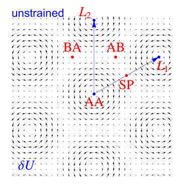
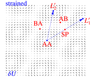
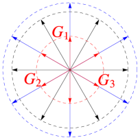
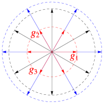
More recently, it also became apparent that an unintentional external heterostrain, i.e. the layer antisymmetric component of strain, has a significant effect on the energy width of the magic angle twisted bilayer graphene narrow bands, and can qualitatively modify the nature of the correlated insulator states [13, 14]. Even for twist angles which, while small, are larger than the magic angle, the moire pattern magnifies the effect of strain [15]. For example, at twist, a heterostrain can lead to change in the real space moire lattice vectors. We illustrate this effect at the magic angle in the Fig. 1 showing the difference between the unstrained moire unit cell lattice vectors and their heterostrained counterparts . Such a large change in atomic lattice constants would be difficult to achieve in a regular material due to the limits on its stability, but are readily observed in twisted bilayer graphene [16, 17, 18, 19, 20]. This phenomenon opens an avenue towards strain engineering the electronic properties of moire materials. For example, Ref. [15] emphasized that even a small, , heterostrain can split the energetic degeneracy of the three van Hove singularities in, say, the conduction moire band and introduce open Fermi surfaces within a finite energy window of the band spectrum, capable of accommodating more than one electron per moire unit cell. The magnetoresistance of the resulting electronic system with open Fermi surfaces can be very large and non-saturating [15]. In contrast, in the absence of the external heterostrain, the van Hove singularities are degenerate and the window of electron filling with open Fermi surfaces shrinks to a point. For these and other reasons, we consider it important to understand the lattice relaxation in the presence of realistic heterostrain.
The purpose of this paper is to provide analytical results which can be used as an input to model the electronic properties of twisted bilayer graphene, with or without heterostrain. In order to have some confidence in the applicability of the theoretical model whose output is the relaxation profile, we first compare the results obtained numerically with the experimentally measured relaxation and strain profiles of twisted bilayer graphene using Bragg interferometry[20] as a function of the twist angle within the range from to . We do this comparison for two theoretical models, Ref.[5] and Ref.[11], and conclude that the results of the model from Ref.[5] follows the experiment much more closely. We therefore focus our attention on obtaining the analytical expressions for the relaxed configuration using the model of Ref.[5].
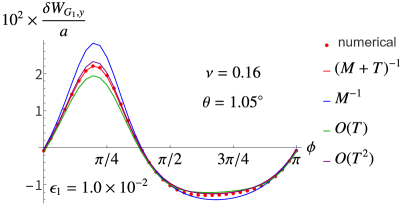
To this end, we introduce a dimensionless parameter that quantifies the ratio between the interlayer adhesion energy and the intralayer elastic energy at a given twist angle (it is precisely defined in the Eq.23). For smaller , is larger due to relative growth of the adhesion energy compared to the elastic energy and leading to a stronger lattice relaxation. At the first magic angle of , the value of reaches . Naively, one may expect that such a small value would allow finding the relaxed configuration by Taylor expanding it in powers of , an approach adopted recently in the Ref.[21]. Interestingly, we find that this approach encounters shortcomings just above the first magic angle. In this regard, we are able to precisely show that although the exact solution for the lattice relaxation is an analytic function of near the origin, the distance to the nearest point of non-analyticity in the complex plane is such that the radius of convergence of the Taylor series is only . This means that including more terms in the Taylor series does not necessarily improve the accuracy of the solution near the magic angle. Instead, we introduce a different method, which allows us to obtain a simple explicit form for the relaxation as a function of , which is highly accurate at, and below, the first magic angle. This approach does not suffer from the problems encountered by the series solution method. Moreover, it can be systematically improved and extended to include external heterostrain. It is sufficiently general to allow for uniaxial and/or biaxial heterostrain that can be treated on equal footing. The analytic formulas we present are accurate to at least heterostrain, and thus within the range of the vast majority of the experimentally examined twisted bilayer graphene devices.
The rest of the paper is organized as follows: in the next subsection we summarize the main result so that the reader can readily find it without needing to go over the details of the derivation. In the section II we set up the formalism to describe twisted and strained honeycomb bilayer, review the expressions for the intralayer elastic energy and the interlayer adhesion energy, and compare the numerical solution for the relaxed configuration with the available experimental data. In the subsection II.1 we present analytical formulas for the relaxed configuration in the absence of external heterostrain, while in the subsection II.2 we calculate the radius of convergence of the series expansion in solution by studying its analytic properties in the complex plane and finding the branch points. In the section III we solve for the relaxed configuration in the presence of external heterostrain. In the section III.1 we discuss the out-of-plane corrugation. The last section contains the discussion.
I.1 Summary of main results
The main result of this paper is the Eq. 61 which gives a formula for the in-plane lattice relaxation of a twisted bilayer graphene subject to an external heterostrain in the Eq.4. The lattice distortion is defined via the Eq. 9, the layer antisymmetric combination in Eq. 10, and the Eq. 18. The three monolayer graphene reciprocal lattice vectors are defined in the Eqs. 2 and 3, and are unaffected by the strain. This is unlike the three moire reciprocal lattice vectors in the Eq. 6. The explicit formulas for the Fourier amplitudes are given in the Eqs.38, 40 and 41, while the additional strain correction is given in the Eq. 60, in terms of Eqs. 56, 57, 58 and 59. The values of the elastic constants and the adhesion energy parameters are provided in the Table 1.
II Lattice Distortion
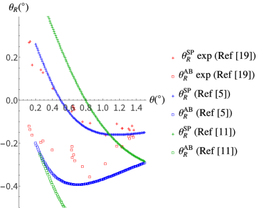
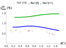
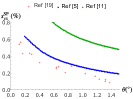
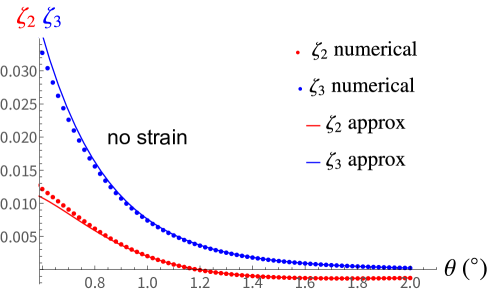
We start by focusing on two different theoretical models for lattice relaxation proposed in Refs. [11, *KoshinoPRB17Erratum] and [5], and compare the distortion obtained numerically from these two models with the experimental measurements of Ref. [20]. The experimental data cover the range of twist angle between and . As shown in the Fig. 2, we find a closer match for the distortion obtained using the model in Ref. [5] than in Ref. [11, *KoshinoPRB17Erratum]. Therefore, in later sections, we choose the model of Ref. [5] to obtain the lattice distortion, not just numerically but also analytically.
Before proceeding with the details of the derivation, we introduce two unit cell vectors of monolayer graphene
| (1) |
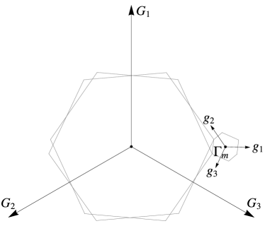
where nm is the magnitude of the monolayer graphene lattice constant. The corresponding reciprocal lattice vectors are
| (2) |
For notational convenience, we also introduce
| (3) |
shown in the Fig. 3(a).
The heterostrain is described by a symmetric matrix . It can always be diagonalized by an orthogonal matrix [17, 7, 15]:
| (4) |
where is the two-dimensional rotational matrix. Note that this rotation has nothing to do with the twist. Rather, the angle determines the orientation of the two principal axes of the strain tensor. are the magnitudes of the strain along the two principal axes. In the case of uniaxial strain along the first principal axis, where is the Poisson ratio [7]. In this work, we also allow for the biaxial strain, therefore, both and are treated as external parameters and we will not assume any specific relation between them. In the presence of experimentally relevant small twist and small heterostrain, the moire lattice vectors , and the corresponding moire reciprocal lattice vectors , can be safely expanded [7] to the linear order in the twist angle and as
| (5) | ||||
| (6) |
The Pauli matrix and is the strain matrix defined in Eq. 4. The full set of the moire reciprocal lattice vectors is given by
| (7) |
with arbitrary integers and . Note that is a non-singular matrix unless the strain and the twist angle are fine-tuned [22]. Thus, we can set up a one-to-one mapping between the set of monolayer graphene reciprocal lattice vectors, , and the set of ’s as
| (8) |
We illustrate this in the Fig. 3(b) and 3(c) in the absence of heterostrain for the first three shells.
As discussed in the Ref. [9], under the assumptions that the lattice distortion on both layers can be approximated by a continuous function whose variation is small on the length scale of , and that the lattice distortion is independent of the graphene sublattice, we can use the Eulerian coordinates to express the distorted in-plane position , on the layer or , via a continuous function of the undistorted position as
| (9) |
Here gives the distortion of the carbon atom due to the twist, the strain, and the relaxation. We start by considering only the (dominant) in-plane lattice relaxation and address the out-of-plane corrugation in Sec. III.1. To proceed, we also introduce the layer symmetric and the layer antisymmetric combination of the in-plane distortions
| (10) |
Although the first-principles approaches have been used to obtain the lattice relaxation [23, 24, 25, 26], the vector fields can be conveniently obtained by minimizing the sum of the elastic energy, , and the interlayer adhesion energy, ,
| (11) |
for example, as done in Refs. [11, 5]. The elastic energy can be expressed in terms of the sum of the layer symmetric and layer anti-symmetric terms
| (12) |
The layer anti-symmetric term is a functional of alone
| (13) |
and the layer symmetric functional , which depends only on can be obtained using
| (14) |
The elastic moduli and are listed in the Table 1. The interlayer adhesion term is a functional of alone. It is given by
| (15) |
where sums over all the reciprocal lattice vectors of monolayer graphene. Note that must be symmetric under various transformations, including the six-fold rotation and the mirror reflection about the -plane, , leading to the following constraints
| (16) | |||
| (17) |
In most theoretical models, is negligible for and thus can be safely ignored outside the first three shells. The interlayer adhesion potential parameters on the first shell, , the second shell, , and the third shell, , for two models proposed in Ref. [5] and Ref. [11, *KoshinoPRB17Erratum] can be found in the Table 1.
Thus, decouples from (see e.g. Ref. [9]). Therefore, minimizing with respect to leads to and . This implies that , where is a constant two-component vector and is a constant. Thus, simply represents an overall rotation of both layers by the same angle of followed by an in-plane translation by the same vector . Such a transformation does not induce any change of the elastic energy and electronic spectrum (unlike the relative twist), and thus we can safely set .
In the presence of a twist by a small angle and a small external heterostrain, can be written as the sum of two terms
| (18) |
where the last term gives the lattice relaxation; is given by Eq. 4. For a uniform twist and an external heterostrain, we seek a moire lattice periodic , with the lattice vectors defined in Eq. 5, i.e. we impose the constraint when minimizing . We are thus tacitly assuming that the substrate stabilizes the “flat” structure and prevents the buckling transition, with bending stiffness collapse and moire translation symmetry breaking, found in the theoretical study of freestanding twisted bilayer graphene in Ref. [27]; our assumption is supported by the data of Ref.[20].
As explained in Ref. [9], the average of over the space can be absorbed by redefining the origin of and thus the average can be set to without loss of generality. Then, can be shown to be odd under space inversion [9], i.e. , leading to its Fourier series
| (19) |
where sums over all the moire reciprocal lattice vectors and are real and odd under . Since Eq. 8 constructs a one-to-one mapping between the moire reciprocal lattice vectors and the reciprocal vectors of the undistorted monolayer graphene lattice, it is sometimes convenient to label the Fourier components using vectors. To this end, we introduce , and the lattice relaxation will also be interchangeably written as .
Minimizing the sum of and leads to the self-consistent equation for (when ):
| (20) |
where is a matrix that can be written as
| (21) |
and is the Fourier series amplitude defined via
| (22) | |||||
The Eq. 20 is a nonlinear equation that can be solved numerically by the iteration method [11, *KoshinoPRB17Erratum, 5, 28, 9, 29]. Tab. 1 lists the parameters for two different models proposed in Ref. [11, *KoshinoPRB17Erratum] and [5] that produce markedly different lattice distortions due to the significant difference in the parameter . Based on these two models, we calculate their local twist produced by the lattice relaxation at two positions: saddle point (SP) stacking at , and AB stacking at , see Fig.1(a), with the twist angle between and . The numerical results for are compared with the experimental measurements of Ref. [20] in the Fig. 2. The measured at the SP point follows the prediction of the model in Ref. [5], but significantly deviates from the prediction of the model in Ref. [11, *KoshinoPRB17Erratum]. Although the calculation in the Fig. 2 is done in the absence of an external strain, including the experimentally estimated heterostrain when for either model does not result in a significant change. The agreement with the data at the AB point is also significantly better for the model of Ref. [5], although it seems to somewhat overestimate at the AB point. This disparity may be related to the experimental measurement, which inherently averages over a particular region around a special point, such as SP, AB, and AA. Our numerical calculations shown in the Fig.2 report the lattice distortion exactly at these special points, without further averaging, and thus always produce stronger distortions than the reported measurements. Therefore, precise details of the inherent averaging in experiments would be needed to further judge the accuracy of the model in Ref. [5]. Comparisons for other distortion parameters are presented in the appendix. Although the mentioned overestimates also occur for other distortion parameters, the overall consistency between the experiments and the model in Ref. [5] persists. In the rest of this manuscript, we will therefore focus on this lattice relaxation model.
II.1 Analytical formula for in-plane relaxation in the absence of external strain
We proceed to derive an approximate but accurate and simple analytical formula for . For this purpose, it is convenient to introduce a dimensionless parameter
| (23) |
that quantifies the ratio between the interlayer adhesion energy and the elastic energy at a given twist angle . For smaller , is larger implying relative growth of the interlayer adhesion energy compared to the elastic energy and leading to stronger lattice relaxation. The theoretical model of Ref. [5] gives at the first magic angle of .
In the unstrained case the moire lattice is invariant under the six-fold rotation and the mirror reflections along and planes. The Helmholtz decomposition of the lattice relaxation field [9] gives
| (24) |
where both fields and are periodic, and even under space inversion, i.e. and . Thus, their Fourier series can be written as
| (25) |
As mentioned, in the absence of external strain, the lattice relaxation is invariant under , and odd under the mirror reflection about and planes, leading to the symmetry constraints for both and . As a consequence, for on the first three shells, must vanish [21], and depends only on the shell index [9],
| (26) | |||
| (27) | |||
| (28) |
In the above we introduced the dimensionless parameters (, , and ) which quantify the strength of on the th shell as . Explicitly displaying the Fourier amplitudes on the first three shells, the lattice distortion field has the form
| (29) |
where for notational simplicity, we define and , , and stand for terms at higher shells than the third.
The solution to the Eq. 20 in the absence of the interlayer adhesion term, , is simple, namely . Therefore, when the adhesion term is small compared to the elastic term, we expect the to be small as well. Assume that we have found this solution. We then extract its amplitude on the first shell and express it in terms of . We can then estimate the magnitudes of the solution on the higher shells, , , etc. in terms of . We see that for small , and given the hierarchy in the Tab.1, the solution for is down by factors of either or compared to . The suppression is even stronger on further shells. Therefore, is almost entirely determined by the Fourier amplitudes on the innermost shell. By solving Eq. 20 numerically using the iteration method, the full solution (which we have at each shell) confirms that for , the Fourier series of is indeed dominated by the innermost shell.
Since is small on the outer shells for the twist angles of interest to us, the Fourier components on the outer shells have a negligible impact on the innermost shell. Consequently, can be obtained accurately by setting in Eq. 29, ignoring the higher shells denoted by the ellipsis, and then minimizing . Explicitly, we start by setting
| (30) |
substituting the above into Eq. 13, and obtaining
| (31) |
where is the total area of the sample. We see that the elastic energy does not depend on the elastic coefficient because on the first -shell is divergence free. The elastic energy cost also grows as a square of the twist angle because the moire period decreases inversely as the twist angle increases and the moire period sets the scale of the spatial variation penalized by the elastic energy. The interlayer adhesion energy, in Eq. 15 can be written as
| (32) |
To perform the Fourier integral we note that the phase factor associated with the distorted configuration is periodic and can be expanded via Fourier series as [30]
| (33) |
where is the Bessel function of the first kind (with integer ). Substituting the above into Eq. 32, we obtain
| (34) |
The last equality has been derived by noting that if and only if is located on the first three shells.
By minimizing with respect to we obtain
| (35) |
Using one can obtain a numerical solution of the above equation which will give the optimal in terms of ; we did so and because we find a highly accurate closed form solution below which matches this numerical solution, we do not show it in Fig. 4.
To proceed analytically we first note that as , the above equation is satisfied if . Physically, this is the limit of short moire period when the elastic energy cost of relaxation dominates the interlayer adhesion energy gain, and the in-plane relaxation vanishes. Therefore, as we increase and increases from zero, we can approximate the right hand side of Eq.35 by Taylor expanding it in small , noting that the Bessel functions of the first kind, , with integer , are entire functions of complex . This is justified as long as the solution for we seek remains small. We find that for , an accurate solution can be obtained by Taylor expanding the right-hand side of Eq.35 in to second order, giving
| (36) |
where for notational convenience, we introduced the parameter
| (37) |
Solving the quadratic Eq.36 gives us an accurate analytical formula for the optimal amplitude on the first shell
| (38) |
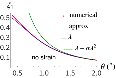
With the parameters listed in Tab. 1 for Ref. [5], we can obtain a numerical solution of Eq. 20. We then extract the corresponding for the relaxation on the -shell using , where and is on the shell. The comparison of such numerical result on the first shell and the approximate formula in Eq. 38 is presented in Fig. 4, showing an excellent agreement for the twist angle down to at least .
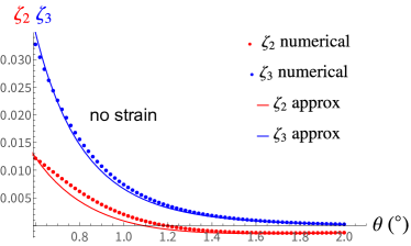
The closed form expressions for the and for the nd and rd shells can be obtained using similar methods. Starting from Eq. 29 with from Eq. 38, we keep fixed and expand the total energy up to the quadratic order of and . This approximation for the energy is justified since and are much smaller than for the twist angle down to , notably smaller than the first magic angle. Integrating Eq. 13 over the space, we found the exact formula for the elastic energy:
| (39) |
We also obtain a (complicated) formula for that is presented in the appendix. Minimizing , and expanding the Bessel functions to , we obtain the approximate solutions for and :
| (40) | ||||
| (41) |
Fig. 4(b) shows the plots of and with parameters specified in Tab. 1 for the model proposed in Ref. [5]. Clearly, the analytical formulas in Eqs. 40 and 41 match with the full numerical solution very well for . In addition, when the (as is the case for ) then as seen from Eq.38, and , confirming our a’priori estimates. Therefore, the Fourier components of the distortion on the outer shells are much smaller than on the first shell, as also confirmed in Fig. 4. This hierarchy in the lattice relaxation not only justifies the assumption when deriving Eq. 40 and 41, but also allows us to neglect the impact of outer shell relaxation on the electronic Hamiltonian for , as shown in an upcoming paper.
We thus obtain a highly accurate expression for the difference between the in-plane layer displacements in the two layers . The accuracy of our formulas for can be further improved. For example, we can expand the right hand side of the Eq.35 to the third order in and solve the corresponding cubic equation for in terms of . We have done so, but because the expressions are somewhat unwieldy and because the Eq.38 is sufficiently accurate for our purposes down to and below the first magic angle, we do not write out the solution of the cubic here. In addition, Eq. 40 and 41 neglect the terms at the order of and . After including such terms, the solution shows an improved agreement with the full numerical solution, as presented in the appendix.
II.2 Radius of convergence for the lattice relaxation
In order to compare with the results of Refs. [30, 21] we expand our solution in the Eq. 38 in a power series of , finding . Although we do not rely on such power series expansion, and in fact discuss its shortcomings below, we note that our leading term agrees with the result obtained in Ref. [30] and Ref.[21] provided we identify the latter’s and with our and respectively. Expanding to such a low order agrees with the full numerical solution on the first shell for , but increasingly overestimates the relaxation at smaller angles; the deviation is at the (first) magic angle. Our prefactor of also agrees with the prefactor in Ref. [21] provided in which case . This prefactor is significantly corrected by non-zero and as shown in Eq. 37, and the resulting prefactor is tiny for the model proposed in Ref. [5].
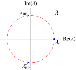
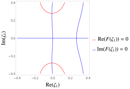
Our closed form solution allows us to understand the convergence of the power series expansion in by studying the analytic properties in the complex plane. The solution in Eq. 38 contains a branch cut with branch points at and . A complex circle centered at the origin and passing through the branch points intersects the real axis at as shown in Fig. 5; is the radius of convergence of the power series [31]. As a consequence, the power expansion of Eq.38 in must diverge if . With the parameters of Ref. [5] specified in Tab. 1, we obtain with the corresponding angle . Note that our solution in the Eq.38 is perfectly smooth at and the singularity occurs only in the power expansion.
Because the right hand side of the Eq.35 is an analytic function of and , we can also study its zeros in the complex plane numerically without approximating the right hand side by a quadratic polynomial in . For a fixed complex value of the zeros of the real part form curves in the complex plane as do the zeros of the imaginary part. Their intersection gives the solutions of the Eq.35, the physical one being on the real axis for real and vanishing with vanishing . For we find that the collision of two solutions closest to the origin occurs for with machine precision and (see Sec. B in Appendix for the method to obtain these and for the proof of the branch points’ existence). These correspond to the branch points we found approximately using Eq.38. For the values of and listed in Tab. 1 for Ref. [5] we find and , further reducing the radius of convergence of any power series in solution to the amplitude of the first shell of . This value of translates to the twist angle placing the first magic angle just outside the radius of convergence and making the power series approach impractical for obtaining an increasingly accurate solution near the first magic angle. As mentioned, our closed form solution does not suffer from this problem. We can further improve upon it by expanding the right hand side of the Eq. 35 to the third order in and solving the corresponding cubic equation for in terms of . We have done so, but because the expressions are somewhat unwieldy and because the Eq.38 is sufficiently accurate for our purposes down to and below the first magic angle, we do not write out the solution of the cubic here.
III Lattice relaxation in the presence of an external Heterostrain
Having discussed the lattice relaxation in the unstrained twisted bilayer, we study the impact of the external heterostrain that is described by a symmetric matrix shown in Eq. 4. Although the heterostrain is ubiquitous in realistic twisted samples, the two strain parameters and are always much smaller than the twist angle in which case the matrix introduced in Eq. 8 is non-singular. As a consequence, the lattice relaxation is still periodic and its periods are given by two non-collinear moire lattice vectors and defined in the Eq. 5. The strained lattice relaxation is obtained by solving Eq. 20 with the corresponding moire reciprocal lattice vectors given in Eq. 6.
Even with the approximation scheme used in the previous section for the unstrained case, it is hopelessly challenging to obtain a closed form solution of the Eq. 20 without making any further assumptions about the magnitude of the heterostrain. Nevertheless, we can make progress by using the fact that in realistic devices the external heterostrain is small i.e. . This can be used to derive an approximate but closed-form solution for the change of lattice relaxation due to external heterostrain. To this end, we express the lattice relaxation as
| (42) |
where ’s are the heterostrain distorted moire reciprocal lattice vectors defined in Eq. 8 and where we introduced to be half of the set of nonzero vectors, that includes one and only one vector for each nonzero vector pair . This can be done because is linear in and is odd under , as discussed below Eq.19. The geometric effect of heterostrain on the reciprocal lattice vectors in the Eq. 8 can be isolated as
| (43) | |||
| (44) |
In addition, we decompose into two parts,
| (45) |
where is the solution of the Eq. 20 in the absence of external heterostrain. It has already been determined in the previous section: for on the first three shells
| (46) |
while for , is too small and thus can be neglected. gives the heterostrain induced change of the Fourier coefficients of the lattice relaxation, , at the reciprocal lattice vectors . Note that these reciprocal lattice vectors are themselves modified by the heterostrain as shown in the Eq.43.
The equation for is obtained by substituting Eq. 43 and 45 into Eq. 20. To present its explicit form, we first decompose the matrix introduced in Eq. 21 into three parts, organized by the powers of ,
| (47) | ||||
| (48) | ||||
| (49) | ||||
| (50) |
Then, as explicitly derived in the Appendix, the Eq. 20 results in the following equation for :
| (51) |
In the above we introduced the function which is most easily defined via a Fourier integral as
| (52) |
Here is the Bessel function of the first kind, the set is introduced in Eq. 42. Of course, the above integral can be performed analytically, but we find it more transparent to present it this way.
So far, no approximations have been made and the obtained nonlinear equation for is still difficult to solve. However, must vanish in the absence of strain. Therefore, for , we expect , leading to As a consequence, the last term in Eq. 51 needs to be known only near the solution, , which we argue is small for small heterostrain. Therefore, the complicated nonlinear term can be approximated by Taylor series in powers of . Expanding it up to the linear order in leads to a set of coupled linear equations for . Since is the solution for the unstrained case, the Eq.51 holds when . The coupled linear equations can be expressed as
| (53) |
where, for notational convenience, we introduced defined as
| (54) |
Note that the first term in the Eq.(53) is a constant, independent of , and the last two terms are linearly proportional to . Therefore, we have successfully transformed the nonlinear equation (51) into a linear equation for . However, due to the infinite number of vectors, the matrix is also of infinite size, and thus needs to be truncated to be practical and to allow obtaining . In the appendix, we present a detailed argument showing that is much larger for on the first shell than on further shells, allowing us to neglect all ’s except (, , and ) in Eq. 53. Thus, we obtain the reduced form of the Eq. 53
| (55) |
where the reduced form of the first term in the Eq. 53, entering the right hand side of the above equation, can be expressed via the heterostrain distorted reciprocal moire lattice vectors in the Eq.6, the reciprocal moire vectors in the absence of the heterostrain , as well as their difference , as
| (56) |
The block diagonal matrix in the Eq. 55 can also be conveniently expressed in terms of ’s and the elastic coefficients and as
| (57) |
Although the matrix with its elements defined as is independent of the external heterostrain, its expression is still quite complicated because of the formally infinite products of infinite sums of Bessel functions. Therefore, further approximations need to be made to the matrix elements in order to obtain the closed-form expression for . Because the unstrained solution is dominated by the first shell, we keep only and set all other ’s to zero. This turns every element of the six-by-six matrix into a nonlinear function of alone. Next, we expand these nonlinear functions up to the order . This effectively truncates the infinite product onto only the first shell of , as well as turns the infinite sum into a finite sum over a manageable number of terms, leading to closed form expressions for the diagonal blocks and the off-diagonal blocks ():
| (58) | ||||
| (59) |
For convenience, here we introduced the notation when , with no sum over repeated indices. As a result, can be solved simply by inverting the matrix , which can always be done analytically using the cofactor method. Thus,
| (60) |
and the heterostrained lattice relaxation can be accurately approximated as
| (61) | |||||
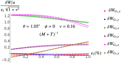
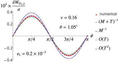
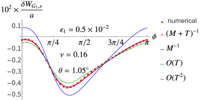
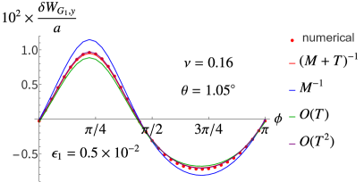
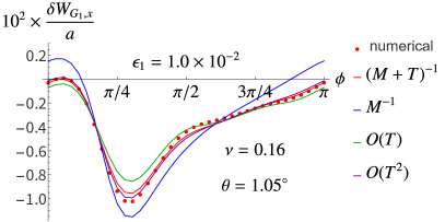
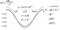
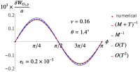
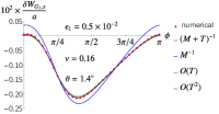
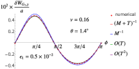
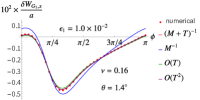
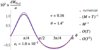
where and , and . Recall that ’s are the heterostrain distorted reciprocal moire lattice vectors in the Eq.6, while ’s are unaffected by the heterostrain (see Eqs. 2,3). If we only keep the first shell, i.e. set , and use from the Eq. 38, then the above result is accurate to within for , and as we shown in an upcoming paper, can be safely used to obtain the electronic spectrum (See also Ref. [32, 33]). Higher accuracy can be achieved by including and from the Eq. 40 and Eq. 41, respectively, allowing us to go below the first magic angle with high accuracy even at . Fig. 6(a) compares the full numerical solution for and our analytical solution in the Eq. 60 for a particular form of the strain matrix with and . As can be seen, the agreement between the two is very good all the way up to , or .
Although the Eq. 60 provides a closed form expression for the heterostrain induced correction to the relaxed atomic configuration, it involves an inverse of the matrix which is cumbersome to express in a simple analytical form. We can further simplify it by noting that there is a hierarchy between the sizes of the matrix – which is simple to invert because it is block diagonal and effectively involves only matrices – and the matrix . Namely, Therefore, when , the inverse of the matrix can be Taylor expanded as
| (62) |
where can be explicitly expressed as
| (63) |
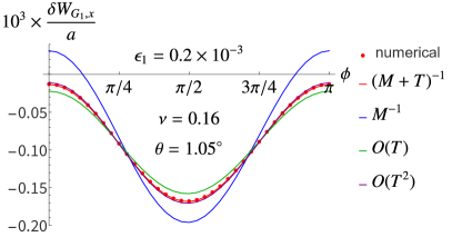
The power series in Eq. 62 can be truncated at any order to produce an approximate closed-form expression for . The accuracy of the truncation order depends on the value of . For , or equivalently , the truncation at th order is highly accurate as shown in the Fig. 11, leading to
| (64) |
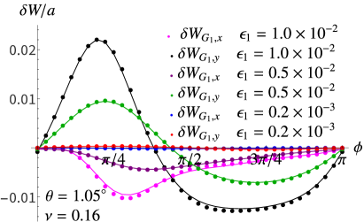
At the first magic angle, the accuracy of different higher order in truncation orders is illustrated in the Fig. 7, where they are compared with the full numerical solution of the Eq. 20 as a function of the strain orientation angle for different values of .
III.1 Lattice Corrugation
In addition to the in-plane relaxation, the atoms of the twisted bilayer graphene also deform along the out-of-plane direction. Such deformation is described by the lattice corrugation field, defined as
| (65) |
where is the lattice distortion on the layer along the out-of-plane direction. is determined by the local interlayer stacking, achieving the maximum at AA stacking and the minimum at AB stacking [34].
The interlayer stacking is given by the relative in-plane distortion . For AA stacking, where are two arbitrary integers and , as defined in Eq. 1, are the monolayer graphene lattice vectors. For AB/BA stacking, . It is straightforward to write the corrugation field as a function of the position as has been done in Eq. 65. However, it is more convenient to express as a function of , i.e. because of its dependence on the interlayer stacking.
The transformation between and is one-to-one for realistic twisted bilayer samples at in which both the external heterostrain and the in-plane relaxation are small compared to . To see this, we use the Eqs. 18 and 19 to compute the Jacobian matrix of this transformation,
| (66) |
As discussed previously, in the absence of the lattice relaxation, must be non-zero for small external heterostrain, proving that in this case the transformation is indeed one-to-one. In the presence of the lattice relaxation, the last term in the Eq. 66 can be estimated to be , and thus can be neglected compared with the term . As a consequence, the above Jacobian determinant is always non-zero, implying that any continuous function can be written as . In the rest of this section, we consider various symmetries which constrain the form of and obtain its approximate formula.
The corrugation field depends on the local interlayer stacking that doesn’t change under the shift (with ). Therefore, is a periodic function , that can be expressed via Fourier series as
| (67) |
If the interlayer stacking is also invariant under and mirror reflections along and planes, then the Fourier components are also unchanged under these transformations. Specifically, is identical at each of the six s on the first shell. Note that for AA stacking and for AB stacking. Approximating by keeping in the Eq. 67 only at and the first shell, i.e. at , we obtain [6]
| (68) |
where the layer antisymmetric in-plane distortion is given by the Eq. 18.
IV summary
In this work, we have compared the lattice relaxation from two models in Ref. [11, *KoshinoPRB17Erratum] and [5] with the experimental results obtained in Ref. [20], and found that the latter model (Ref. [5]) follows the experimental data much more closely. Using this model we then derived a closed form expression for the lattice relaxation. In the absence of external heterostrain, we found our analytical expression for the lattice relaxation which is highly accurate for the twist angles down to . Introducing the dimensionless parameter that quantifies the ratio between the interlayer adhesion energy and the elastic energy at a given twist angle, we also found that when the lattice relaxation is expanded in the Taylor series in , it becomes divergent at a value of which translates to the twist angle slightly above the magic value for realistic models of the elastic energy and the interlayer adhesion energy. We related this divergence to the existence of the branch points of the solution in the complex plane, and numerically determined the radius of convergence of the Taylor series with high precision.
We also derived a closed form expression for the strain-induced change of the lattice relaxation. This formula is accurate at least up to heterostrain. It can be used to understand the electronic spectrum of the twisted bilayer graphene in the presence of realistic heterostrain. Incorporating these results into the electronic continuum model will be a subject of an upcoming paper.
Acknowledgements.
J. K. acknowledges the support from the NSFC Grant No. 12074276, the Double First-Class Initiative Fund of ShanghaiTech University, and the start-up grant of ShanghaiTech University. O.V. was funded in part by the Gordon and Betty Moore Foundation’s EPiQS Initiative Grant GBMF11070 and acknowledges support from the National High Magnetic Field Laboratory funded by the National Science Foundation (Grant No. DMR-2128556) and the State of Florida.References
- Cao et al. [2018a] Y. Cao, V. Fatemi, A. Demir, S. Fang, S. L. Tomarken, J. Y. Luo, J. D. Sanchez-Yamagishi, K. Watanabe, T. Taniguchi, E. Kaxiras, R. C. Ashoori, and P. Jarillo-Herrero, Nature 556, 80 (2018a).
- Cao et al. [2018b] Y. Cao, V. Fatemi, S. Fang, K. Watanabe, T. Taniguchi, E. Kaxiras, and P. Jarillo-Herrero, Nature 556, 43 (2018b).
- Bistritzer and MacDonald [2011] R. Bistritzer and A. H. MacDonald, Proc. Natl. Acad. Sci. USA 108, 12233 (2011), https://www.pnas.org/doi/pdf/10.1073/pnas.1108174108 .
- Fang and Kaxiras [2016] S. Fang and E. Kaxiras, Phys. Rev. B 93, 235153 (2016).
- Carr et al. [2018a] S. Carr, D. Massatt, S. B. Torrisi, P. Cazeaux, M. Luskin, and E. Kaxiras, Phys. Rev. B 98, 224102 (2018a).
- Koshino et al. [2018] M. Koshino, N. F. Q. Yuan, T. Koretsune, M. Ochi, K. Kuroki, and L. Fu, Phys. Rev. X 8, 031087 (2018).
- Bi et al. [2019] Z. Bi, N. F. Q. Yuan, and L. Fu, Phys. Rev. B 100, 035448 (2019).
- Kang and Vafek [2018] J. Kang and O. Vafek, Phys. Rev. X 8, 031088 (2018).
- Kang and Vafek [2023] J. Kang and O. Vafek, Phys. Rev. B 107, 075408 (2023).
- Carr et al. [2018b] S. Carr, D. Massatt, S. B. Torrisi, P. Cazeaux, M. Luskin, and E. Kaxiras, Phys. Rev. B 98, 224102 (2018b).
- Nam and Koshino [2017] N. N. T. Nam and M. Koshino, Phys. Rev. B 96, 075311 (2017).
- Nam and Koshino [2020] N. N. T. Nam and M. Koshino, Phys. Rev. B 101, 099901 (2020).
- Kwan et al. [2021] Y. H. Kwan, G. Wagner, T. Soejima, M. P. Zaletel, S. H. Simon, S. A. Parameswaran, and N. Bultinck, Phys. Rev. X 11, 041063 (2021).
- Parker et al. [2021] D. E. Parker, T. Soejima, J. Hauschild, M. P. Zaletel, and N. Bultinck, Phys. Rev. Lett. 127, 027601 (2021).
- Wang et al. [2023a] X. Wang, J. Finney, A. L. Sharpe, L. K. Rodenbach, C. L. Hsueh, K. Watanabe, T. Taniguchi, M. A. Kastner, O. Vafek, and D. Goldhaber-Gordon, Proc. Natl. Acad. Sci. USA 120, e2307151120 (2023a), https://www.pnas.org/doi/pdf/10.1073/pnas.2307151120 .
- Huder et al. [2018] L. Huder, A. Artaud, T. Le Quang, G. T. de Laissardière, A. G. M. Jansen, G. Lapertot, C. Chapelier, and V. T. Renard, Phys. Rev. Lett. 120, 156405 (2018).
- Kerelsky et al. [2019] A. Kerelsky, L. J. McGilly, D. M. Kennes, L. Xian, M. Yankowitz, S. Chen, K. Watanabe, T. Taniguchi, J. Hone, C. Dean, A. Rubio, and A. N. Pasupathy, Nature 572, 95 (2019).
- Xie et al. [2019] Y. Xie, B. Lian, B. Jäck, X. Liu, C.-L. Chiu, K. Watanabe, T. Taniguchi, B. A. Bernevig, and A. Yazdani, Nature 572, 101 (2019).
- Wong et al. [2020] D. Wong, K. P. Nuckolls, M. Oh, B. Lian, Y. Xie, S. Jeon, K. Watanabe, T. Taniguchi, B. A. Bernevig, and A. Yazdani, Nature 582, 198 (2020).
- Kazmierczak et al. [2021] N. P. Kazmierczak, M. Van Winkle, C. Ophus, K. C. Bustillo, S. Carr, H. G. Brown, J. Ciston, T. Taniguchi, K. Watanabe, and D. K. Bediako, Nat. Mater. 20, 956 (2021).
- Ezzi et al. [2024] M. M. A. Ezzi, G. N. Pallewela, C. De Beule, E. J. Mele, and S. Adam, Phys. Rev. Lett. 133, 266201 (2024).
- Sinner et al. [2023] A. Sinner, P. A. Pantaleón, and F. Guinea, Phys. Rev. Lett. 131, 166402 (2023).
- Guinea and Walet [2019] F. Guinea and N. R. Walet, Phys. Rev. B 99, 205134 (2019).
- Cantele et al. [2020] G. Cantele, D. Alfè, F. Conte, V. Cataudella, D. Ninno, and P. Lucignano, Phys. Rev. Res. 2, 043127 (2020).
- Leconte et al. [2022] N. Leconte, S. Javvaji, J. An, A. Samudrala, and J. Jung, Phys. Rev. B 106, 115410 (2022).
- Gargiulo and Yazyev [2018] F. Gargiulo and O. V. Yazyev, 2D Materials 5 (2018).
- Wang et al. [2023b] J. Wang, A. Khosravi, A. Silva, M. Fabrizio, A. Vanossi, and E. Tosatti, Phys. Rev. B 108, L081407 (2023b).
- Ochoa [2019] H. Ochoa, Phys. Rev. B 100, 155426 (2019).
- Xie and Liu [2023] B. Xie and J. Liu, Phys. Rev. B 108, 094115 (2023).
- Ceferino and Guinea [2023] A. Ceferino and F. Guinea, 2D Materials 11 (2023).
- Whittaker and Watson [1996] E. T. Whittaker and G. N. Watson, A course of modern analysis (Cambridge University Press, 1996) pp. 91–94.
- Herzog-Arbeitman et al. [2024] J. Herzog-Arbeitman, J. Yu, D. Călugăru, H. Hu, N. Regnault, O. Vafek, J. Kang, and B. A. Bernevig, Heavy fermions as an efficient representation of atomistic strain and relaxation in twisted bilayer graphene (2024), arXiv:2405.13880 [cond-mat.mes-hall] .
- Herzog-Arbeitman et al. [2025] J. Herzog-Arbeitman, D. Călugăru, H. Hu, J. Yu, N. Regnault, J. Kang, B. A. Bernevig, and O. Vafek, Kekulé spiral order from strained topological heavy fermions (2025), arXiv:2502.08700 [cond-mat.str-el] .
- Uchida et al. [2014] K. Uchida, S. Furuya, J.-I. Iwata, and A. Oshiyama, Phys. Rev. B 90, 155451 (2014).
Appendix A Comparison with the experiments
In this section, we compare the experiments reporting the lattice relaxation with the calculated relaxation from two different theoretical models proposed in Ref. [11] and [5]. Instead of using the closed-form solution for lattice relaxation, we numerically solve the self-consistent equation (Eq. 20) using the iteration method to obtain the lattice relaxation for these two theoretical models.
Fig. 2 in the main text illustrates the relaxation-induced twist, defined as , at the SP and AB stacking points, for both the experiment and the calculation from two theoretical models. The experimental measurement is more consistent with the model proposed in Ref. [5]. As a consequence, this model is chosen to derive the closed form of the lattice relaxation with and without external heterostrain. In addition, this model is also used in upcoming works to study the electronic continuum model and the strain-induced change of the electron spectrum. In this section, we compare other quantities of the relaxation at high symmetry points. Based on the comparison of these quantities, the same conclusion is drawn that the model proposed in Ref. [5] is more consistent with the experimental measurements.
The derivative of the lattice relaxation is a rank- tensor that contains four independent components. The antisymmetric part gives the local twist as defined in the main text. The symmetric part contains three independent parameters, and can be diagonalized by an orthogonal matrix.
| (69) |
where is the matrix describing the rotation along axis with the rotation angle of , and both and are the magnitudes of strain along two principle axes. Note that all the parameters , , and are position dependent. In addition to , Ref. [20] has introduced several quantities to describe the lattice relaxation.
| (70) |
where is the principle angle giving the orientation of the two principle axes of the strain matrix.

Appendix B Branch points
As discussed in Sec. II.1, can be obtained by solving Eq. 35. The equation can be rewritten as
| (71) | |||
| (72) |
In principle, for fixed , the nonlinear equation contains multiple solutions for . The physical one is given by the solution that approaches as , and therefore, is well-defined at least for small . In addition, the solution contains branch points in the complex plane, whose magnitude gives the radius of convergence. is a highly nonlinear function, and therefore approximation methods are needed to derive the explicit expression of in terms of . The closed form of in Eq. 38 is obtained by expanding to the order of , which works very well for real and real . However, due to the different convergence behavior of with the complex argument , relatively larger errors are introduced for complex and thus for complex . Consequently, Eq. 38 cannot provide precise values of the branch points and the resulting radius of convergence. In this section, we provide a different method to obtain the branch points without explicitly expressing in terms of .
Note that at the branch points,
| (73) |
Expanding the equation around the branch points , we obtain
| (74) |
Substituting and into the above equation, we find
| (75) |
that gives the approximate solution of when close to branch points. Around the branch points, cannot be uniquely solved, therefore
where in the last step, we substituted from the relation . Introducing
| (76) |
with defined in Eq. 72. The zero points of the function give at the branch points. Since the explicit formula of has already been given in Eq. 72, can also be explicitly expressed as a nonlinear function. The numerical value of complex can be accurately obtained by various numerical methods. Consequently, can be obtained by Eq. 73. Fig. 9 shows two colored curves where the real part (in red) and the imaginary part (in blue) of vanish respectively on the complex plane. The crossing points of these two colored curves give . As illustrated in the plot, the two crossing points are stable against any small change of the parameters in the function , and thus the existence of these two branch points is robust.
Appendix C Higher order components of unstrained lattice relaxation
In this section, we derive the approximate closed form of the Fourier components at the second and the third shells. Note that the lattice relaxation can thus be approximated as
| (77) |
where we have introduce the variable and for notational convenience. Correspondingly, the elastic energy can be simplified as
| (78) |
Note that can be obtained by minimizing the sum of elastic energy and interlayer adhesion potential energy, with being fixed to be the solution of Eq. 36. For small and , we expand the interlayer adhesion potential up to the quadratic order of and . Note that the th order has already been calculated to solve . At the linear order of and , we obtain
| (79) |
Expanding to the order of , we found
| (80) |
The full quadratic order of the interlayer adhesion energy is too complicated to write down here. If we keep only the term in the adhesion potential and expand to the order of , we obtain
| (81) |
Expand to and differentiating with respect to and , we obtain,
| (82) |
where
| (83) | ||||
| (84) | ||||
| (85) | ||||
| (86) | ||||
| (87) |
Solving this equation, we obtain and as a function of . For , we have
| (88) |
Appendix D Impact of external heterostrain
In this section, we derive the equation for , especially the expression of in Eq. 52. Notice that Eq. 20 is still valid in the presence of external heterostrain. As shown in Eq. 47 – 50, the matrix is decomposed into the sum of three parts ordered by the powers of and gives the first term of Eq. 51. In addition, since , we have
| (89) |
The Fourier components of can be expressed as
| (90) |
Then, the right hand side of Eq. 20 can be written as
| (91) | ||||
| where | ||||
| (92) |
This gives the definition of , same as Eq. 52.
As explained in the main text, can be approximately obtained by solving the matrix equation , where the matrix is given by Eq. 47. At large twist angle , , and thus we can neglect matrix. For other cases, especially when , becomes sizable, and thus we achieve a higher accuracy when we do not neglect the matrix. We thus expand the inverse matrix using the power series in ,
| (93) |
where the obtained at different truncation orders are illustrated in Fig 7 for and Fig. 11 for .
D.1 Dominance of the first shell for the heterostrained lattice relaxation
This subsection focuses on the estimates of with small strain. We will argue that for on the first shell is much larger than other s. For notational convenience, we introduce the variable,
| (94) |
When strain is small, , and thus . Also, we generalize the variable introduced in Eq. 56 as
| (95) |
with the subscript for all reciprocal lattice vectors. Consequently, can be written in the form of
| (96) |
As the first step, we estimate the magnitude of each term in Eq. 96. From Eq. 47 –50, and note that , it is found
| (97) |
As a consequence, for small strain,
| (98) |
On the other hand, the upper bound of the matrix elements can be estimated as
| (99) |
Clearly, when , the above matrix elements are much smaller than the magnitude of the matrix elements, leading to the expansion of ,
| (100) |
In addition, due to the hierarchy structure of in Eq. 98, for at the shell,
| (101) |
where Eq. 46 is used in the last step.
As a result, obtains the same hierarchy structure as for the unstrained lattice relaxation. Especially, (for , , and ) are much larger than other on outer -shells. Thus, for on the first shell,
| (102) |
For on the -shell with , using Eq. 100, we obtain
| (103) |
where , , and are in-plane spatial indices. Combining Eq. 97, 99, and 101, and noticing for at the first several momentum shells, we conclude that
| (104) | |||
| (105) |
Because of the hierarchy structure of for the unstrained case, and , estimated in Eq. 102 is found to be much larger than of the outer shell estimated in Eq. 105, allowing us to keep only (with , and ) and obtaining Eq. 55.
Appendix E Symmetry constraints
Most of the symmetries of the unstrained moire system, including the six-fold rotation along axis, and mirror reflections along and planes, are broken by the presence of external heterostrain. Consequently, these transformations no longer impose constraints on the explicit form of the strained lattice relaxation, but interestingly, can still relate the lattice relaxations at different heterostrain orientations. Such relations play a crucial role in understanding the change of the electronic spectrum by strain, which we plan to address in upcoming papers. In this section, we will derive these relations.
As shown in Eq. 4, the heterostrain is described by three parameters: , , and . Therefore, in this subsection, the strain matrix is labeled as , and correspondingly, the reciprocal lattice vectors are labeled as
| (106) |
Similarly, we label the lattice relaxation as . Since , by the definition of in Eq. 4, , implying that the strain matrix and thus the lattice relaxation are periodic functions of with the same periods of . The same is true for , the Fourier components of
| (107) |
In addition, by Eq. 4,
| (108) |
Since and thus commutes with , Eq. 8 gives
| (109) |
The set of vectors, which is unaffected by the heterostrain, is invariant under . By setting in the above formula, for two heterostrains and , we conclude that the two sets of the corresponding moire reciprocal lattice vectors are related by rotation. Since ,
| (110) |
Since both the elastic energy and the interlayer adhesion potential are invariant under , we conclude
| (111) |
leading to their corresponding Fourier components related by
| (112) |
In particular, for at the innermost shell, we obtain
| (113) | |||
| (114) |
Combining Eq. 107, 113, and 114, we conclude that by varying from to already provides (, , and ) with arbitrary angle .
In addition, the strain matrix also satisfies the relation
| (115) | ||||
| (116) |
where is the mirror reflection along plane, that transforms an arbitrary in-plane vector to . As shown in Fig. 3, the set of all vectors is invariant under both and . Thus, for two heterostrains described by and , Eq. 116 demonstrates that the two sets of the corresponding moire reciprocal lattice vectors are related by the mirror reflection . Notice that
| (117) |
Since both and are invariant under , we conclude
| (118) |
and the corresponding Fourier components satisfy
| (119) |
Although Eqs. 111, 112, 118, 119 are derived with external heterostrain, they are also valid in the absence of heterostrain by setting . The obtained formulas give the constraints on and the corresponding Fourier components for the unstrained system, as have been derived in Ref. [9].