Optimization of path-integral tensor-multiplication schemes in open quantum systems
Abstract
Path-integral techniques are a powerful tool used in open quantum systems to provide an exact solution for the non-Markovian dynamics. However, the exponential tensor scaling with memory length of these techniques limits the applicability when applied to systems with long memory times. Here we provide an optimization scheme which effectively reduces the tensor sizes by using a matrix representation and singular value decomposition to neglect negligible contributions. This approach dramatically reduces both computational time and memory usage of the traditional tensor-multiplication schemes. Calculations that would require over 50 million GB of RAM in the original approach are now available on standard desktop computers, allowing access to new regimes and more complex systems. As a demonstration, we apply it to the Trotter decomposition with linked cluster expansion technique, and use it to investigate a quantum dot- microcavity system at larger coupling strengths than previously achieved. Secondly, we apply the optimization when the memory time is very long - specifically in a system containing two spatially separated quantum dots in a common phonon bath.
I Introduction
The decoherence and phenomena such as energy relaxation dynamics of open quantum systems is characterized by the interaction between the system and its surrounding environment (bath). In the simplest case, the system-environment coupling is weak and it can be assumed that the environment lacks memory (i.e., is Markovian) and remains uncorrelated with the system. This assumption allows the use of Born and Markov approximations [1, 2, 3] resulting in a time-local equation of motion. This is valid because the effect of the environment on the system occurs on a much larger timescale than the correlation time of the environment. However, many quantum systems deviate from this idealized case, where memory effects play a critical role and render the Born-Markov approximation invalid. In such non-Markovian regimes, the system’s evolution depends on its past interactions, leading to complex phenomena [4, 5, 6, 7]. Accurately capturing these non-Markovian effects is essential but comes with significant computational challenges, often limiting the scope of treatable systems and coupling regimes.
The typical approaches to solving the dynamics in non-Markovian open quantum systems can broadly be divided into perturbative and non-perturbative methods. For example, in a quantum dot (QD)-cavity system coupled to a bath of acoustic phonons, the perturbative treatments are typically limited to specific parameter regimes, e.g. when the QD exciton is not very strongly coupled to the cavity mode, the effect of phonons may be addressed perturbatively [8]. Or, via the polaron transformation combined with a perturbation theory [9, 10]. However, for stronger coupling, phonons play a more significant role that requires non-perturbative techniques [11].
In contrast, non-perturbative techniques, such as Feynman’s path integral formulation is very well suited for system-bath dynamics as it avoids dealing with the large Hilbert space of the bath by targeting the system’s reduces density matrix (RDM). The formulation takes into account the effects of a harmonic bath on the system dynamics through the well known Feynman-Vernon influence functional [12], valid for any system-bath coupling strength. In practice, the issue is that the influence functional is nonlocal in time, meaning that the coordinates of a path at any particular time point are connected to coordinates at every time point, leading to full entanglement. As a consequence, there is an exponential scaling of the computational resources with propagation time, restricting the dynamics to only short times. However, there is a finite length to the non-local interactions contained in the influence functional, known as the memory time, leading to the development of the iterative quasi-adiabatic propagator path integral (i-QuAPI) approach [13, 14, 15, 16, 17, 18]. This finite memory time results in a linear scaling of the computational time with the number of propagations (time steps). The i-QuAPI approach is a tensor-multiplication scheme based on the combined use of Trotter’s decomposition and the Feynman-Vernon influence functional. Due to the finite memory time, it can be used to evaluate the dynamics of the reduced density matrix for an arbitrary time length, not limited to short times. However, as it involves tensors, where each element corresponds to a specific “path” the system could take, the computational memory requirement grows exponentially as the number of time steps included in the memory is increased, also known as the number of neighbors. The memory storage requirements can quickly become too large and in some systems convergence is not possible. To address this, filtering techniques [19, 20, 21], modified truncation schemes [22], path segment merging (MACGIC-iQuAPI) [23], and in some regimes blip decomposition [24, 25] have been developed to offer improvements to the storage requirements or extend the applicability to longer memory times. However, there is still great difficulty in accurately modeling systems where memory effects from the environment are significant, such as energy transfer processes with long coherence times (e.g., photosynthetic complexes) or multi-qubit decoherence in structured environments [26, 27].
More recently, approaches utilizing modern tensor network (TN) techniques such as the Time-Evolving Matrix Product Operator (TEMPO) algorithm [28] (more recently packaged as OQuPY [29]) have provided exceptional reductions in memory requirements. Although TEMPO can achieve many neighbors, the singular value decomposition (SVD) threshold must be decreased as the number of neighbors increases to ensure an accurate calculation, which in turn increases computational resource demands. Or the ACE algorithm [30], another TN approach which further reduces requirements by concentrating only on the most relevant degrees of freedom of the bath. An enhanced TEMPO algorithm has also been developed to include an off-diagonal system bath coupling to the Hamiltonian, leading to multi-time correlations for a two-level system [31] and beyond [32].
Another path-integral based, numerically exact tensor multiplication scheme, developed in parallel, is the Trotter decomposition with linked cluster expansion technique developed in [33]. This has been used in several cases, such as the FWM polarization in quantum dot-cavity systems [34], the linear polarization in multi-qubit systems [27], and the population dynamics in Förster coupled QDs [35]. However, being a tensor multiplication scheme, it also suffers from the exponential scaling with time steps included in the finite memory time.
In this paper, we provide an intuitive optimization scheme to the propagator and influence functional tensors used in path-integral approaches to solve for the exact quantum dynamics in open quantum systems. We use the Trotter decomposition with linked cluster expansion technique as a demonstration. For illustration, we specifically apply it to simplest case of the linear optical polarization (coherences) in a QD-cavity system described in [33], allowing us to provide simple diagrams to intuitively explain the optimization scheme. Although the optimization is applicable to systems of any basis size or other density matrix elements, and has been applied to the population dynamics in Förster coupled QDs [35]. The optimization remaps the tensors as matrices, while maintaining all possible paths, and employs singular value decomposition to compress the matrices, reducing computational resources. The reduction in memory requirements results in approximately twice the number time steps included in the finite memory time than previously available. This provides better accuracy in systems with longer memory times and access to new parameter regimes. For reference, to achieve the new level of accuracy using the original method, it would require over 50 million GB of RAM. We also apply an extrapolation procedure that approximates the exact () long-time dynamics which requires sufficient data generated by the optimization scheme. Furthermore, in cases where calculations are already well converged using the original tensor-multiplication scheme, the optimization provides substantial time savings, often improving efficiency by at least factor of 30. We firstly use the optimization scheme to investigate the dephasing rates in a QD-cavity system in a coupling strength regime not yet explored. Secondly, we show the necessity of the optimization scheme in systems with very long memory times, using a system of two spatially separated QDs coupled to a common phonon bath as demonstration. Physically, the long memory times are due to the shared bath, where phonons may travel between the QDs and the larger the dot separation, the larger the memory time.
II System Hamiltonian
This optimization can be applied to systems consisting of any number of two-level systems (TLSs) that are directly coupled and interact with an environment, either a shared one or independent environments. Additionally, they may interact with an arbitrary number of micro-cavities.
The general form of Hamiltonian that is treatable is (in units of ):
| (1) |
describes the coupling between the TLSs and the TLS-cavity coupling strengths, and is given by:
| (2) |
where represents the system Hamiltonian of the TLSs, where the diagonal elements () correspond to the excitation energy of the TLS at site , , while the off-diagonal elements (, for ) describe the direct coupling between TLSs at sites and , . The operator creates an excitation in the two-level system at site and a photon in a cavity mode , has energy and is created by the operator . The TLS at site is coupled to a cavity mode with strength . The bath consists of bosons in three dimension with energies
| (3) |
where creates an excitation in the bath with wave vector q. The TLS-bath interaction is given by :
| (4) |
where describes the interaction strength of the TLS at site with bath mode in bath . Eq. (4) can be used to describe the scenario where multiple TLSs are coupled to the same bath, or coupled to their own independent baths. The diagonal TLS-bath coupling is needed for an exact calculation using linked cluster expansion, however recently it was also shown that the path-integral based approaches can also be efficiently used for non-diagonal coupling [32].
This general model can be reduced to describe many physical systems by choosing the number of TLSs and turning on/off specific coupling terms, such as energy transport in biological systems [36, 37], qubits in microwave resonators [38, 39], quantum dots interacting with a micromechanical resonator [40], and spin-qubit systems [41].
The specific implementation of the TLSs considered in this paper are semiconductor QDs which are coupled to an environment modeled as a bath of acoustic phonons. Although the general Hamiltonian detailed above describes the range of problems this optimization can treat, we reduce the Hamiltonian into two cases for illustration. Case 1 A QD-cavity system coupled to a bath of acoustic phonons detailed in [33], and Case 2 a QD-QD-cavity system coupled to the same phonon bath, detailed in [27].
The coupling of the exciton in a QD at site to the phonon mode q is given by the matrix element , which depends on the material parameters and exciton wave function, and for multiple QDs in the same phonon bath, the position of the QD. Their explicit form for isotropic QDs is provided in Appendix LABEL:App:Coupling. Importantly, for Case 2 describing a pair identical coupled QDs in a shared environment, separated by a distance vector d, the matrix elements satisfy an important relation
| (5) |
which is the source of long memory times, due to the QD separation. Physically, the long memory times are due to the shared bath, where phonons may travel between the QDs. So, the memory time can be as long as the phonon coherence time, and the larger the dot separation, the larger the memory time, which manifests itself as a delay in the bath correlation functions.
III Path-integral approach
|
|
|
For illustration we consider the linear optical polarization as a simple quantum correlator to investigate, although any element of the density matrix, and other quantum correlators may be considered, such as the FWM polarization [34] or populations, which has already been done in [35]. The linear optical polarization where and denote, respectively, the excitation channel at and measurement channel at the observation time , is given by by definition, where is the full density matrix. As has been derived in Ref. [33], the linear polarization can written as
| (6) |
where is the evolution operator and denotes the expectation value over all phonon degrees of freedom in thermal equilibrium. Common to path-integral based approaches, the time interval , where is the observation time, is split into equal steps of duration , where the time represents the time at the -th step. Trotter’s theorem is then used to separate the time evolution of the two non-commuting components of the Hamiltonian, and . In fact, applying Trotter’s decomposition theorem, the time evolution operator can be written as
| (7) |
where . The final exponent in Eq. (7) describes the dynamics of the system in the absence of phonons and is written as an operator :
| (8) |
However, the necessity of the path-integral approach arises due to the exciton-phonon interactions in Eq. (7) which can be handled in various ways but always results in a tensor multiplication scheme of some form, which the optimization scheme can be applied to. In particular, we choose to apply linked cluster expansion [43]. This leads the tensor multiplication scheme used in [33, 34, 27, 35]:
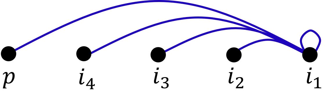
| (9) |
where is known as the propagator and is the full influence functional, and Fig. 1 shows the path segments contained in the tensors. The role of is to propagate the system forward in time, taking the tensor to , where contains all correlations contained within the memory time. captures how past states influence the present dynamics, incorporating non-Markovian effects. The number of correlations, or time steps, included in the tensor is also referred to as the number of neighbors, , with Fig. 1 depicting neighbors. Each index in the tensor can have possible values, for example, in a QD-QD-cavity system, Case 2, , where correspond to the excitonic channels in QD or , respectively, and represents the cavity channel. At any time step within the memory kernel, the excitation can transfer between these components, meaning that evolves dynamically as the system oscillates between QD , QD , and the cavity. In Fig. 1, shows a specific case of two-time correlations, employed in all of the path-integral techniques mentioned so far. This is a consequence of the assumption that the system-bath coupling is bilinear, in which case all higher-order correlation functions can be expressed in terms of the two-time correlations and is given by
| (10) |
where denotes a cumulant arising from the application of linked cluster expansion [43]. The cumulants contain two indices, , describing the two-time correlations between two time points and , the full detailed method is outlined in [27].
The initial full influence functional at the first time step simply is given by , where is the excitation channel and is given by Eq. (8). This is because after excitation in channel at (), one further time step introduces index , which has several possible paths of evolution.
Finally, the linear optical polarization is given by
| (11) |
The subscript represents the indices are placed into the cavity channel at the given time steps, but more generally this is any channel uncoupled to phonons, such as the ground absolute ground state of the system. As the number of time steps within the memory kernel increases (increasing neighbors), the tensors in Eq. (9) are growing exponentially in size. The exponential growth limits the number of correlations that can be considered, due to computational limitations. As a consequence, calculations in systems with long memory times or strong coupling regimes—where the dynamics exhibit rapid oscillations—face limitations in achieving convergence.
IV Optimization scheme
As a simple example, we demonstrate the optimization scheme in Case 1: The linear polarization in a QD-cavity system. Already studied in [33], this system requires two basis states () such that indicates the system is in the cavity (exciton) state at time step .
We write the equations for a general number of neighbors, but within the diagrams only neighbors () to ease understanding.
The core principle of the optimization scheme focuses on mapping the tensors in Eq. (9) to matrices, then SVDing at each time step to truncate the size. Let us consider the first time step, after excitation in channel at . In this case, the full influence functional tensor can be fully populated by , given by Eq. (8) and then mapped to a matrix :
| (12) |
The mapped matrix is populated by only two values, or . This is because after excitation in channel at , one further time step introduces index , which has two possible paths of evolution, and . Although the indices corresponding to later time steps () do not exist yet at the first time step, we include them as a placeholder for subsequent propagation.
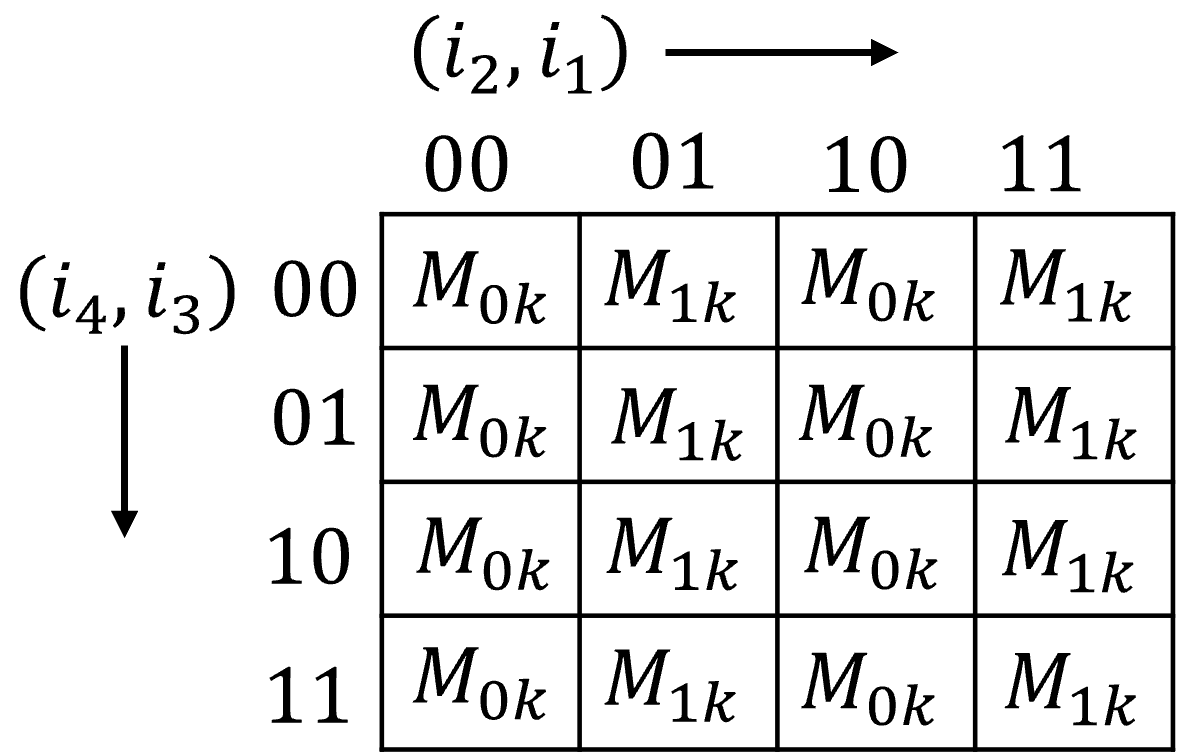
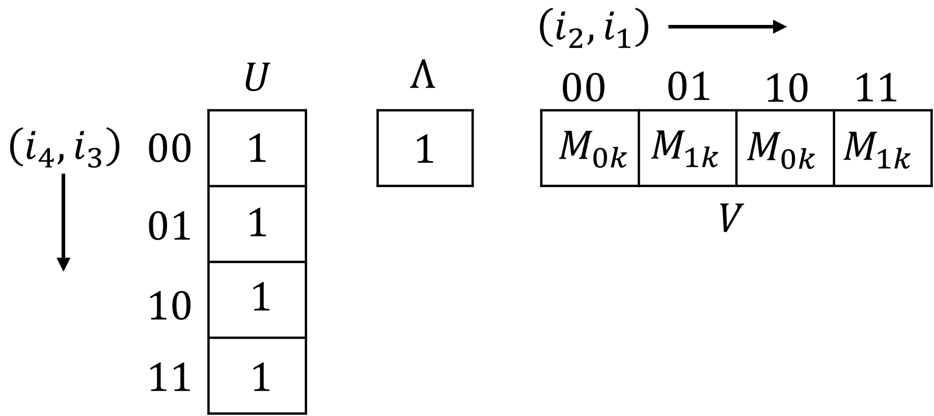
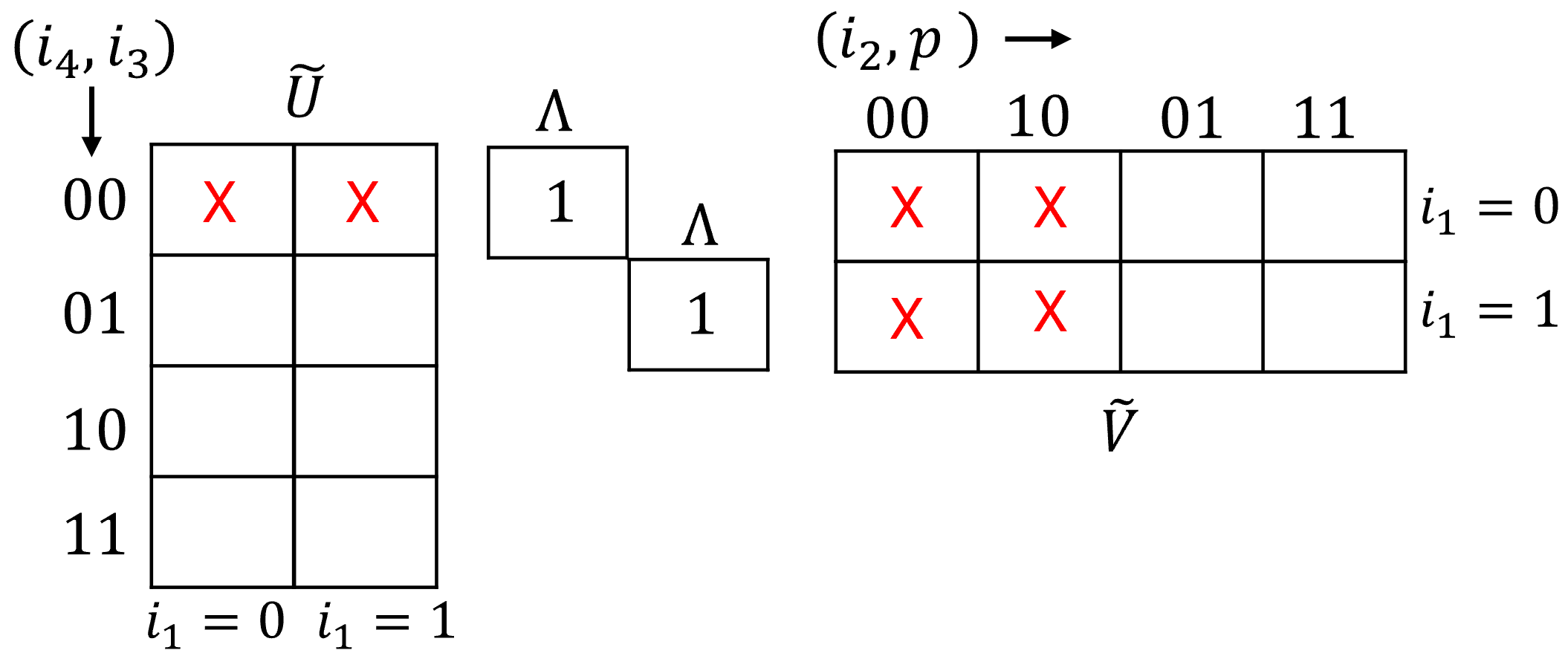
In , the columns take into consideration the possible values of the indices , and the rows add , as depicted in Fig. 2. Since the linear polarization in the QD-cavity system only has the possible index options and , for indices there are permutations to take into account, each permutation represents a possible path of the system as it evolves over the time steps. For , the permutations are simply 00,01,10,11. Thus, the dimensions of the mapped matrix , are ,. However, contains the same number of elements as the original tensor , and therefore providing no memory usage reduction. To remedy this, in order to avoid constructing large tensors in the first instance, can be analytically expressed in SVD form. In general, this is always possible to do, and is given by:
| (13) |
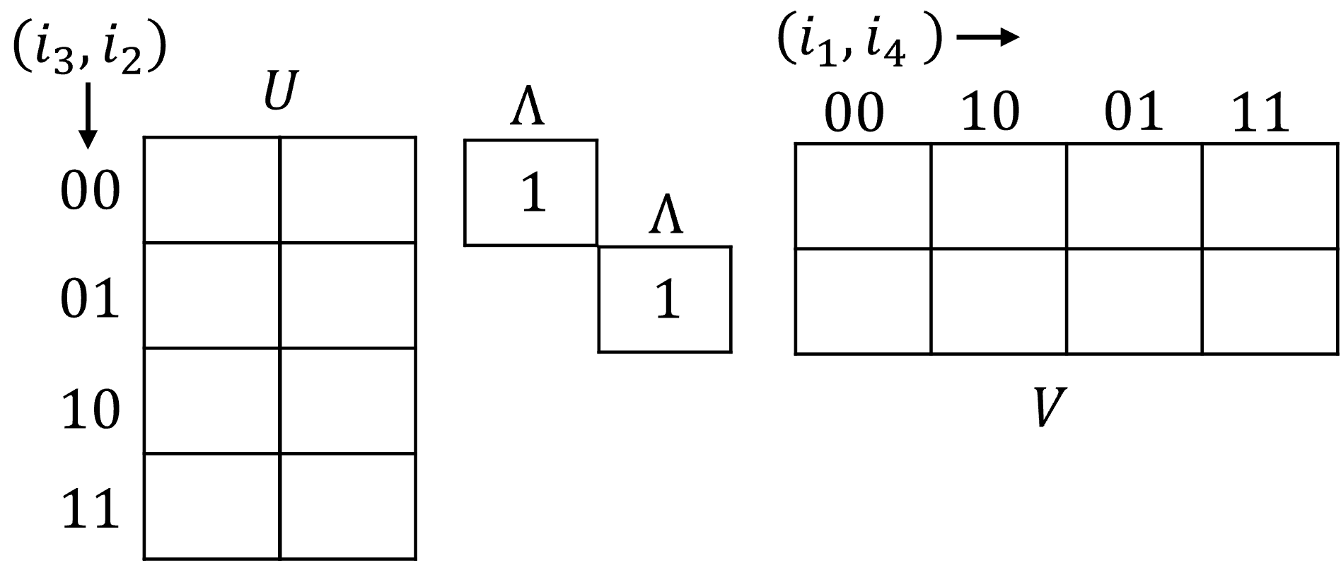
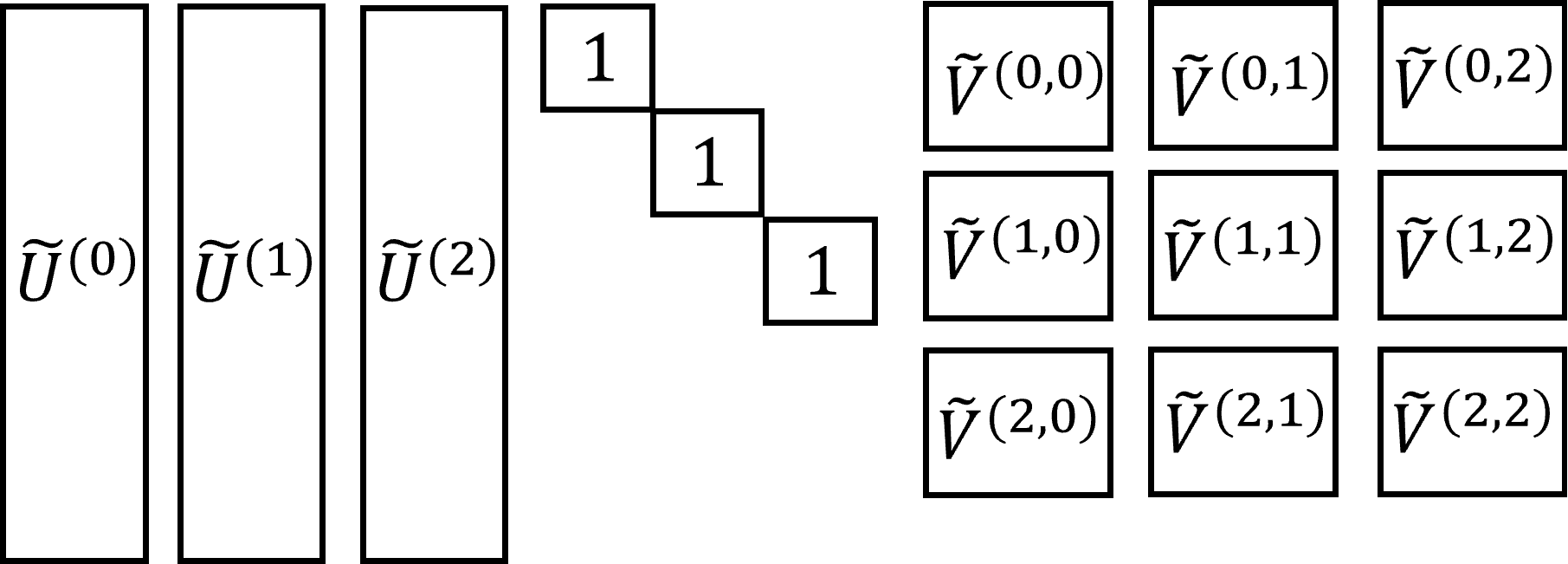
with , and . Fig. 3 shows the matrix in SVD form. This reduces the total number of elements from to , having a significant impact at larger , approximately doubling the amount of neighbors accessible. As the matrix has now been split due to the SVD, we define a column matrix which takes into account the indices and the row matrix, , taking into account indices .
For further time steps, the exciton-phonon coupling has to be considered, which is taken in to account via the propagator in Eq. (9). is successively applied to propagate the system forward in time, summing over the first index, , as seen in Eq. (9).
Although the propagator Eq. (10) is in the form of a tensor, the two-time correlations can be expressed as matrices in the following way
| (14) | ||||||
The recursive relation Eq. (9), can be re-expressed as
| (15) |
The product of the matrices must be applied to the appropriate elements of , with a summation over index . To perform the summation over , let us separate into and components,
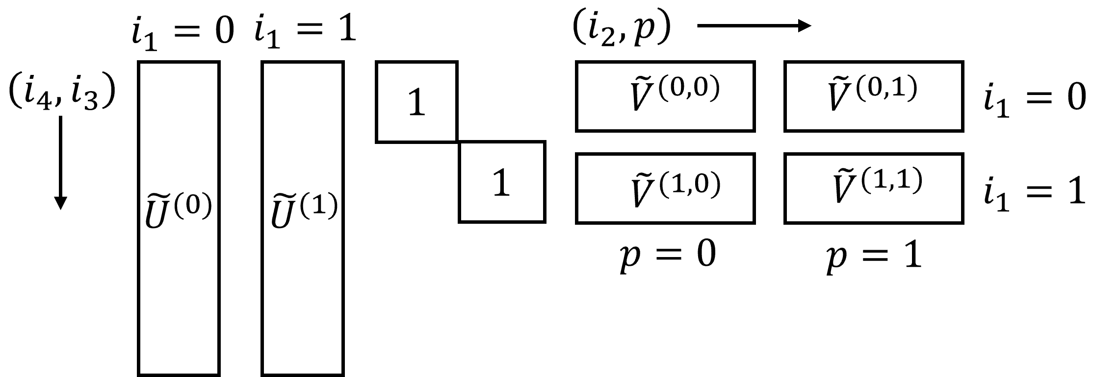
| (16) |
where if and if . With reference to Fig. 3, since has no dependence on , is the same in both cases, but if and if , where . At this point, the product of matrices can be multiplied into and . The matrices which contain correlations between indices contained within , i.e. and will be multiplied into . Note that since contains no information about , both possibilities of and must be taken into account. The matrices which contain correlations between and indices are multiplied with . However, due to the propagator containing the additional index , we choose to apply onto the matrix, but as there is no information about index , both possibilities of and must be taken into account. We then obtain two new matrices,
| (17) |
corresponding to and , respectively. Similarly,
| (18) |
with or , due to the introduction of the new index in Eq. (15), which is necessary for the forward propagation of the system in time. For example, the matrix means we apply the element to elements in that correspond to and , and to the elements corresponding to and , and so on.
Now, a new matrix representing in Eq. (15) takes the form
| (19) |
Where the tilde notation denotes that the matrices have been applied, propagating the system forward in time for this iteration. The new propagated matrix at step is shown diagrammatically in Fig. 4. In Fig. 4, and have been split due to the summation over , according to Eqs. (17) and (18), and the matrices in Eq. (IV) have been applied, further splitting due to the introduction of a new index in the propagator.
To calculate the polarization, given in Eq. (11) at a particular time step, we take the specific realization , where is the measurement channel. Fig. 5 shows the matrices in Fig. 4 more explicitly, with the red crosses indicating which elements should be multiplied together for this specific realization. This matrix multiplication is effectively summation over , as required, and the measurement channel, , is selected by choosing . The realization ( ) is obtained through standard matrix multiplication with the elements in final row of with the column corresponding to the permutation column in , corresponding to the cavity (exciton) observation channel. Note that the permutation ordering changes, as has taken the place of so that varies across rows, not columns for the matrix multiplication to effectively sum over , as required.
In the recursion relation Eq. (15), must become the new for the next time step, effectively cycling the indices. As an example, for , becomes associated with and with . After each time step, we redefine () as () as seen in Fig. 6, indicating that the splitting due to and must take place again and subsequent multiplication of the matrix elements to propagate the system. In the following time step, the indices will again cycle, but once the index becomes associated with , the original index ordering has been restored but on opposite matrices. Therefore, at this point, it’s computationally simpler to transpose all the matrices such that and , allowing us to return to the original procedure at the first iteration. After iterations, the matrices should be transposed in order to return the indices to their original positions, that is, associated with , we call this the start of the cycle.
It is clear that through the splitting due to and after each time step, the size of matrix doubles in size relative to the previous step, and through the splitting due to and , also doubles in size. Thus, every subsequent doubles in size, however this can be optimized by applying SVD.
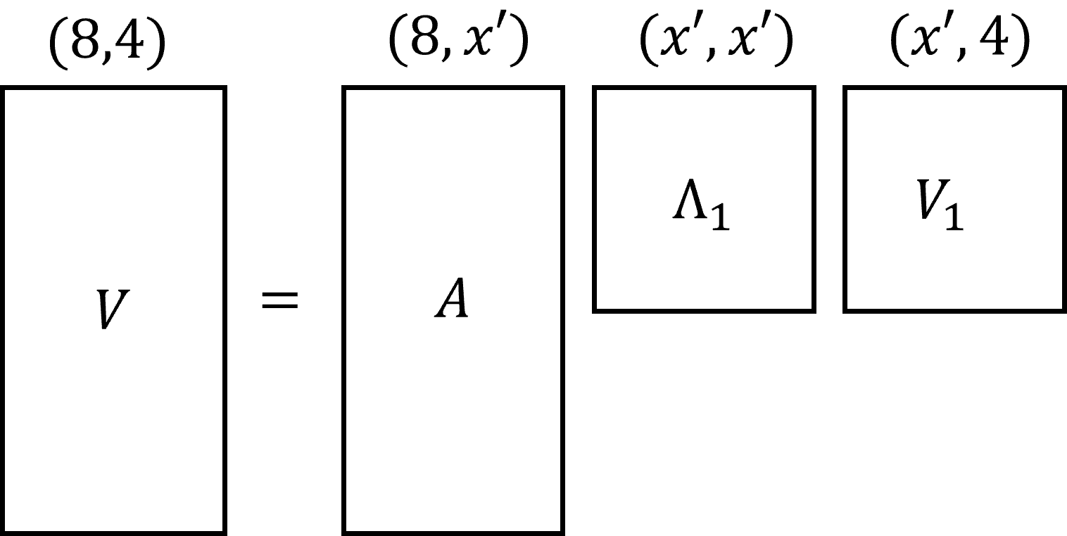
For instance, we can SVD , where containing the significant values has a smaller size due to the threshold condition that if then , truncating the SVD matrices. The threshold may be changed based on the desired accuracy of the calculation, the results in this paper typically use , where is the largest value contained in . as, seen in Fig. 7, consider for illustration , which is initially a matrix at the first time step, but has increased to an matrix after three iterations for . Then, if after applying the threshold only values remain, would be a matrix, is , is .
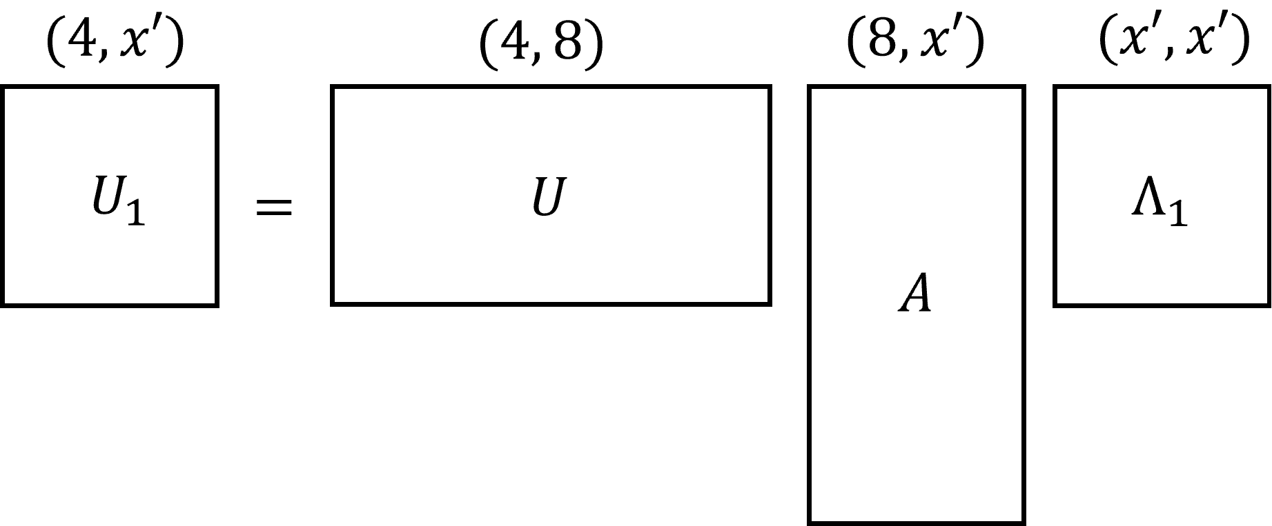
Initially this appears to increase the number of required elements, however and can be multiplied into , which is a matrix, and through just matrix multiplication, the size of is truncated to . If the truncation is insufficient after one application, one can SVD and multiply the products into . Effectively, there is an SVD sweeping back and forth to truncate the sizes. These truncated matrices are then used as the starting and for the following time step, with the SVD procedure applied every time step to keep the matrices from growing exponentially.
Computationally the procedure is straightforward, we start with a tensor which has a number of indices equal to the amount of time steps within the memory kernel. We then assign half the indices to a matrix , and the other half to matrix , where each element corresponds to a specific path, or permutation, of the indices. Due to the exponential form of the propagator, it can be decomposed into matrices, , which describe the correlations between two time points. Since each element in and describe a specific path of the system, the value of the indices are known the appropriate matrix element can be multiplied into and . Then via matrix multiplication of the desired rows and columns, a specific realization is calculated and any physical observable can be found. The exponential scaling of the matrix sizes is then handled via SVD sweeping.
IV.1 Generalization to J-dimensional density matrix vectors
More generally for a system and correlator which can be fully described by system states, The dimensions of the mapped matrix, and , are dependent on the number of neighbors, and , i.e. for even , . In other words, there are more permutations for more possible system states.
At time step , the tensor (where ) is represented by a standard matrix . As before, the indices are assigned to the matrices and , however, due to the extra possible states of , the matrix is split into matrices , each corresponding to a specific realization. is a times smaller matrix than since the values are known, as this index is associated with . The propagation index also has possible values, and each is duplicated to account for all possible values. Similarly, is duplicated times, with each corresponding to a possible realization, as there is no information about index contained within . Fig. 9 shows the specific case of , which may represent Case 2, the linear polarization in a QD-QD-cavity system. The matrices defined in Eq. (IV) are applied into the correct positions as before, and there is a summation over , propagating the system from to . Denoting the propagated full influence functional tensor as the mapped matrix , we have
| (20) |
with
| (21) |
as before, but with .
V Verification
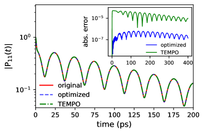
Fig. 10 illustrates the accuracy of our optimization scheme by calculating the linear optical polarization of an isotropic QD coupled to a micro-cavity with coupling strength eV. The parameters of InGaAs QDs studied in [44, 45] are used: eV, where () is the conduction (valence) band deformation potential, m/s is sound velocity, is the mass density, the confinement length nm, and the temperature is K. We compare the results from the original full tensor multiplication scheme [33], the optimized calculation, and the well-known TEMPO approach [28] using the same number of neighbors, in each case. An SVD threshold of is used in the optimized and TEMPO calculations. The inset of Fig. 10 demonstrates the error between the full well-converged original calculation and the optimization (blue) and TEMPO (green). The inset shows the close agreement between the optimized scheme and the original full tensor method confirms the validity of our approach, while the comparison with TEMPO serves as an additional point of reference. There is a large benefit to computational time, taking roughly 1300 seconds using the original approach, compared with only 40 seconds using the optimization scheme. The maximum achievable neighbors in the original full calculation for this QD-cavity system is for a desktop PC of GB RAM, whereas the optimized case has approximately , at most.
VI Extrapolation
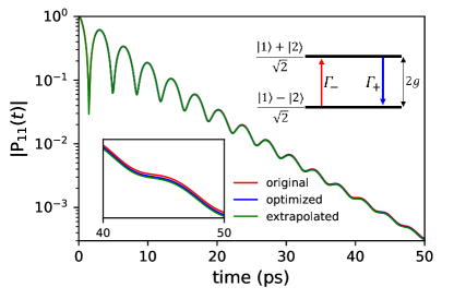
As detailed in [33, 27], the strong coupling between the exciton and cavity forms a polariton, and the oscillatory behavior in Fig. 10 is explained by the coherent exchange of energy between the polariton states. The energy levels of the states are separated by the Rabi splitting, which determines the beat frequency in . This frequency physically represents the exchange of quantum information between the QD and the cavity. The temporal decay of the linear polarization expresses the decoherence in this system as a consequence of the interaction of the QD with the bath. This decoherence is due to phonon-assisted transitions between the upper () and lower () polariton states (see Sec. VII.1 and [27]).
With this picture in mind, we have applied to the long-time dynamics of a biexponential fit of the form
| (22) |
extracting the complex amplitudes , energies , and dephasing rates of the phonon-dressed polariton states. These extracted parameters follow a power law of convergence with the number of neighbors . Therefore, one can calculate the linear optical polarization for a given number of neighbors, then apply a fit to the long time data and extract the fit parameters. The resulting parameters across the range of neighbors are used to perform a power-law extrapolation, estimating the exact value which corresponds to .
As an example, consider the parameters corresponding to the dephasing rates, extracted across a range of neighbors, with the convergence of to the exact () value is assumed to follow a power law model, given by:
| (23) |
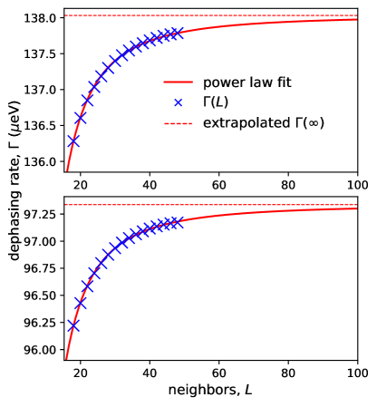
Figure 11 shows the calculated values (blue crosses) in the QD-cavity system, with the power law model applied (red curve), and the extrapolated is shown as a red dashed line. The value of is estimated for the values of shown in Fig. 11 by minimizing the root mean square deviation from the power law Eq. (23) for . Fig. 11 also demonstrates the necessity of the extrapolation, since optimization alone may not be well converged in some cases. However, the extra data provided by the optimization by achieving more neighbors allows for an accurate usage of the extrapolation. In fact, in some systems with very long memory times, such as in extended quantum systems, the extrapolation is not possible at all with the original technique and requires the optimization.
VII Results
VII.1 Accessing stronger coupling regimes in the QD-cavity system
Fig. 12 shows the linear optical polarization of an isotropic QD coupled to a micro-cavity with coupling strength eV at zero detuning.
The data is calculated with the original tensor-multiplication scheme, the optimization and extrapolation. There is good convergence of the original calculation at this coupling strength because the time step , which decreases as the number of neighbors increases, is small enough to resolve the dynamics of the Rabi oscillations. The frequency of the Rabi oscillations at zero detuning is determined by the energy splitting of between the polariton states (see inset of Fig. 12). Therefore, as increases, a smaller time step is required for an accurate calculation. The optimization and extrapolation thus provides access to larger coupling strengths.
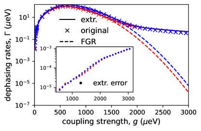
Fig. 13 shows the dephasing rates in the QD-cavity system as a function coupling strength . The optimized and extrapolated data visually align with the original calculation at smaller coupling strengths, but show a deviation at larger values as expected. Provided that the parameters extracted via the optimization scheme follow the power law convergence, the extrapolated values are accurate for significantly larger coupling strengths than the original approach. The inset of Fig. 13 shows the extrapolated error for each of the extrapolated values, where even at eV the extrapolated error is much less than the difference between the extrapolated and original calculations.
VII.2 Necessity of the optimization in spatially extended systems
When a spatially extended quantum system interacts with a common environment, the memory time can become very large and the dynamics are difficult to capture accurately. We now use Case 2, a system of two spatially separated QDs coupled to a microcavity and interacting with a shared phonon bath as illustration.
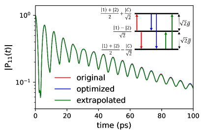
Fig. 14 shows the linear polarization, , for a pair of cavity-mediated (eV) coupled isotropic QDs separated by nm. In this case of zero detuning () and equal QD-cavity couplings, there are three resulting mixed states, and , as depicted in the inset (see [27]). To generate the extrapolated data, a triexponential fit is applied to to extract the parameters of these mixed states. Fig. 14 compares the original, optimized and extrapolated calculations, however, the separation of nm is small and does not significantly increase the memory time (see [27]). Therefore, we observe a similar and sufficient convergence of the original calculation as in the QD-cavity system in the previous section.
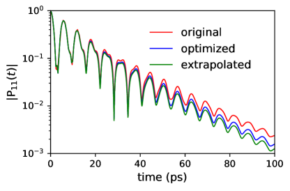
Fig. 15 shows the same calculation, but instead with a separation of nm, which displays a clear lack of convergence using the original method. Even the calculation using the optimization scheme is not very well converged, showing the necessity of the extrapolation. It should be noted that the extracted parameters do not follow a power-law convergence across all values, instead, the selected values must be sufficiently high to enter the regime of power-law convergence. Due to this, the original technique in most regimes of spatially extended systems cannot generate enough data within the power-law convergence regime to provide an extrapolated calculation. Therefore, the optimized calculations are required for the extrapolation, although even this is insufficient for coupling strengths over eV paired with large QD separations over nm.
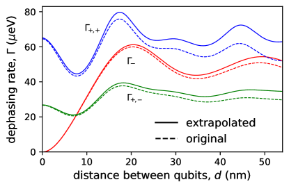
Fig. 16 shows the dephasing rates extracted from the fit as functions of the QD separation . The dephasing rates of the mixed states and are denoted by and , respectively. As the QD separation increases, the memory time increases, and the original calculation gradually becomes increasingly inaccurate, requiring the optimization and extrapolation to accurately model the system.
VIII Conclusion
In conclusion, we have developed an optimization scheme for path-integral tensor-multiplication schemes used to compute the exact dynamics in non-Markovian open quantum systems. We demonstrate the scheme by investigating the linear polarization in a quantum dot-cavity system, and verify the scheme by comparison with the full original approach and the well-known TEMPO algorithm. The scheme approximately doubles the number of neighboring connections within the tensor network structure, which is significant given the exponential scaling associated with tensor multiplication schemes. The increased number of neighbors provides better convergence in large coupling strength regimes, and for systems with long memory times. Furthermore, calculations already well converged using the traditional approach, our optimization scheme offers greatly improved computational efficiency, shortening calculation time by more than times and reducing the memory usage by over times.
Acknowledgments
L.H. acknowledges support from the EPSRC under grant no. EP/T517951/1.
References
- Breuer and Petruccione [2002] H.-P. Breuer and F. Petruccione, The Theory of Open Quantum Systems (Oxford University Press, Oxford ; New York, 2002).
- De Vega and Alonso [2017] I. De Vega and D. Alonso, Dynamics of non-Markovian open quantum systems, Rev. Mod. Phys. 89, 015001 (2017).
- Breuer et al. [2016] H.-P. Breuer, E.-M. Laine, J. Piilo, and B. Vacchini, Colloquium : Non-Markovian dynamics in open quantum systems, Rev. Mod. Phys. 88, 021002 (2016).
- Krummheuer et al. [2002] B. Krummheuer, V. M. Axt, and T. Kuhn, Theory of pure dephasing and the resulting absorption line shape in semiconductor quantum dots, Phys. Rev. B 65, 195313 (2002).
- Hohenester et al. [2009] U. Hohenester, A. Laucht, M. Kaniber, N. Hauke, A. Neumann, A. Mohtashami, M. Seliger, M. Bichler, and J. J. Finley, Phonon-assisted transitions from quantum dot excitons to cavity photons, Phys. Rev. B 80, 201311 (2009).
- Stock et al. [2011] E. Stock, M.-R. Dachner, T. Warming, A. Schliwa, A. Lochmann, A. Hoffmann, A. I. Toropov, A. K. Bakarov, I. A. Derebezov, M. Richter, V. A. Haisler, A. Knorr, and D. Bimberg, Acoustic and optical phonon scattering in a single In(Ga)As quantum dot, Phys. Rev. B 83, 041304 (2011).
- Reiter et al. [2019] D. E. Reiter, T. Kuhn, and V. M. Axt, Distinctive characteristics of carrier-phonon interactions in optically driven semiconductor quantum dots, Advances in Physics: X 4, 1655478 (2019).
- Kaer et al. [2010] P. Kaer, T. R. Nielsen, P. Lodahl, A.-P. Jauho, and J. Mørk, Non-Markovian Model of Photon-Assisted Dephasing by Electron-Phonon Interactions in a Coupled Quantum-Dot–Cavity System, Phys. Rev. Lett. 104, 157401 (2010).
- Ramsay et al. [2010] A. J. Ramsay, A. V. Gopal, E. M. Gauger, A. Nazir, B. W. Lovett, A. M. Fox, and M. S. Skolnick, Damping of Exciton Rabi Rotations by Acoustic Phonons in Optically Excited InGaAs / GaAs Quantum Dots, Phys. Rev. Lett. 104, 017402 (2010).
- Nazir and McCutcheon [2016] A. Nazir and D. P. S. McCutcheon, Modelling exciton–phonon interactions in optically driven quantum dots, J. Phys.: Condens. Matter 28, 103002 (2016).
- Hughes et al. [2011] S. Hughes, P. Yao, F. Milde, A. Knorr, D. Dalacu, K. Mnaymneh, V. Sazonova, P. J. Poole, G. C. Aers, J. Lapointe, R. Cheriton, and R. L. Williams, Influence of electron-acoustic phonon scattering on off-resonant cavity feeding within a strongly coupled quantum-dot cavity system, Phys. Rev. B 83, 165313 (2011).
- Feynman et al. [2010] R. P. Feynman, A. R. Hibbs, and D. F. Styer, Quantum Mechanics and Path Integrals, emended ed ed., Dover Books on Physics (Dover publ, Mineola, 2010).
- Makarov and Makri [1994] D. E. Makarov and N. Makri, Path integrals for dissipative systems by tensor multiplication. Condensed phase quantum dynamics for arbitrarily long time, Chemical Physics Letters 221, 482 (1994).
- Makri and Makarov [1995a] N. Makri and D. E. Makarov, Tensor propagator for iterative quantum time evolution of reduced density matrices. II. Numerical methodology, The Journal of Chemical Physics 102, 4611 (1995a).
- Makri and Makarov [1995b] N. Makri and D. E. Makarov, Tensor propagator for iterative quantum time evolution of reduced density matrices. I. Theory, The Journal of Chemical Physics 102, 4600 (1995b).
- Makri [1995] N. Makri, Numerical path integral techniques for long time dynamics of quantum dissipative systems, Journal of Mathematical Physics 36, 2430 (1995).
- Shao and Makri [2001] J. Shao and N. Makri, Iterative path integral calculation of quantum correlation functions for dissipative systems, Chemical Physics 268, 1 (2001).
- Shao and Makri [2002] J. Shao and N. Makri, Iterative path integral formulation of equilibrium correlation functions for quantum dissipative systems, The Journal of Chemical Physics 116, 507 (2002).
- Sim and Makri [1997] E. Sim and N. Makri, Filtered propagator functional for iterative dynamics of quantum dissipative systems, Computer Physics Communications 99, 335 (1997).
- Sim [2001] E. Sim, Quantum dynamics for a system coupled to slow baths: On-the-fly filtered propagator method, The Journal of Chemical Physics 115, 4450 (2001).
- Lambert and Makri [2012] R. Lambert and N. Makri, Memory propagator matrix for long-time dissipative charge transfer dynamics, Molecular Physics 110, 1967 (2012).
- Liu et al. [2024] L. Liu, J. Ren, and W. Fang, Improved Memory Truncation Scheme for Quasi-Adiabatic Propagator Path Integral via Influence Functional Renormalization (2024), arXiv:2406.01978 [physics] .
- Richter and Fingerhut [2017] M. Richter and B. P. Fingerhut, Coarse-grained representation of the quasi adiabatic propagator path integral for the treatment of non-Markovian long-time bath memory, The Journal of Chemical Physics 146, 214101 (2017).
- Makri [2014] N. Makri, Blip decomposition of the path integral: Exponential acceleration of real-time calculations on quantum dissipative systems, The Journal of Chemical Physics 141, 134117 (2014).
- Makri [2017] N. Makri, Iterative blip-summed path integral for quantum dynamics in strongly dissipative environments, The Journal of Chemical Physics 146, 134101 (2017).
- Gribben et al. [2020] D. Gribben, A. Strathearn, J. Iles-Smith, D. Kilda, A. Nazir, B. W. Lovett, and P. Kirton, Exact quantum dynamics in structured environments, Phys. Rev. Research 2, 013265 (2020).
- Hall et al. [2024] L. M. J. Hall, L. S. Sirkina, A. Morreau, W. Langbein, and E. A. Muljarov, Controlling dephasing of coupled qubits via shared-bath coherence (2024), arXiv:2405.14685 [cond-mat] .
- Strathearn et al. [2018] A. Strathearn, P. Kirton, D. Kilda, J. Keeling, and B. W. Lovett, Efficient non-Markovian quantum dynamics using time-evolving matrix product operators, Nat Commun 9, 3322 (2018).
- Fux et al. [2024] G. E. Fux, P. Fowler-Wright, J. Beckles, E. P. Butler, P. R. Eastham, D. Gribben, J. Keeling, D. Kilda, P. Kirton, E. D. C. Lawrence, B. W. Lovett, E. O’Neill, A. Strathearn, and R. de Wit, OQuPy: A Python package to efficiently simulate non-Markovian open quantum systems with process tensors, The Journal of Chemical Physics 161, 124108 (2024), arXiv:2406.16650 [quant-ph] .
- Cygorek and Gauger [2024] M. Cygorek and E. M. Gauger, ACE: A general-purpose non-Markovian open quantum systems simulation toolkit based on process tensors (2024), arXiv:2405.19319 .
- Jørgensen and Pollock [2019] M. R. Jørgensen and F. A. Pollock, Exploiting the Causal Tensor Network Structure of Quantum Processes to Efficiently Simulate Non-Markovian Path Integrals, Phys. Rev. Lett. 123, 240602 (2019).
- Richter and Hughes [2022] M. Richter and S. Hughes, Enhanced TEMPO algorithm for quantum path integrals with off-diagonal system-bath coupling: Applications to photonic quantum networks, Phys. Rev. Lett. 128, 167403 (2022), arXiv:2110.01334 [quant-ph] .
- Morreau and Muljarov [2019] A. Morreau and E. A. Muljarov, Phonon-induced dephasing in quantum-dot–cavity QED, Phys. Rev. B 100, 115309 (2019).
- Sirkina and Muljarov [2023a] L. S. Sirkina and E. A. Muljarov, Impact of the phonon environment on the nonlinear quantum-dot–cavity QED: Path-integral approach, Phys. Rev. B 108, 115312 (2023a).
- [35] L. S. Sirkina, L. M. J. Hall, A. Morreau, W. Langbein, and E. A. Muljarov, Förster transfer between quantum dots in a shared phonon environment: A rigorous approach, revealing the role of pure dephasing (In Preparation).
- Chin et al. [2013] A. W. Chin, J. Prior, R. Rosenbach, F. Caycedo-Soler, S. F. Huelga, and M. B. Plenio, The role of non-equilibrium vibrational structures in electronic coherence and recoherence in pigment–protein complexes, Nature Phys 9, 113 (2013).
- Rey et al. [2013] M. D. Rey, A. W. Chin, S. F. Huelga, and M. B. Plenio, Exploiting Structured Environments for Efficient Energy Transfer: The Phonon Antenna Mechanism, J. Phys. Chem. Lett. 4, 903 (2013).
- Blais et al. [2004] A. Blais, R.-S. Huang, A. Wallraff, S. M. Girvin, and R. J. Schoelkopf, Cavity quantum electrodynamics for superconducting electrical circuits: An architecture for quantum computation, Phys. Rev. A 69, 062320 (2004).
- Zheng and Baranger [2013] H. Zheng and H. U. Baranger, Persistent Quantum Beats and Long-Distance Entanglement from Waveguide-Mediated Interactions, Phys. Rev. Lett. 110, 113601 (2013).
- Yeo et al. [2014] I. Yeo, P.-L. De Assis, A. Gloppe, E. Dupont-Ferrier, P. Verlot, N. S. Malik, E. Dupuy, J. Claudon, J.-M. Gérard, A. Auffèves, G. Nogues, S. Seidelin, J.-P. Poizat, O. Arcizet, and M. Richard, Strain-mediated coupling in a quantum dot–mechanical oscillator hybrid system, Nature Nanotech 9, 106 (2014).
- Childress et al. [2006] L. Childress, M. V. Gurudev Dutt, J. M. Taylor, A. S. Zibrov, F. Jelezko, J. Wrachtrup, P. R. Hemmer, and M. D. Lukin, Coherent Dynamics of Coupled Electron and Nuclear Spin Qubits in Diamond, Science 314, 281 (2006).
- Sirkina and Muljarov [2023b] L. S. Sirkina and E. A. Muljarov, Impact of the phonon environment on the nonlinear quantum-dot cavity QED. II. Analytical approach (2023b), arXiv:2306.16579 [cond-mat] .
- Mahan [2000] G. D. Mahan, Many-Particle Physics (Springer US, Boston, MA, 2000).
- Muljarov and Zimmermann [2004] E. A. Muljarov and R. Zimmermann, Dephasing in Quantum Dots: Quadratic Coupling to Acoustic Phonons, Phys. Rev. Lett. 93, 237401 (2004).
- Muljarov et al. [2005] E. A. Muljarov, T. Takagahara, and R. Zimmermann, Phonon-Induced Exciton Dephasing in Quantum Dot Molecules, Phys. Rev. Lett. 95, 177405 (2005).