CDGS: Confidence-Aware Depth Regularization for 3D Gaussian Splatting

Abstract

3D Gaussian Splatting (3DGS) has shown significant advantages in novel view synthesis (NVS), particularly in achieving high rendering speeds and high-quality results. However, its geometric accuracy in 3D reconstruction remains limited due to the lack of explicit geometric constraints during optimization. This paper introduces CDGS, a confidence-aware depth regularization approach developed to enhance 3DGS. We leverage multi-cue confidence map of monocular depth estimation and sparse Structure-from-Motion (SfM) depth to adaptively adjusts depth supervision during the optimization process. Our method demonstrates improved geometric detail preservation in early training stages and achieves competitive performance in both NVS quality and geometric accuracy. Experiments on the public available Tanks and Temples benchmark dataset show that our method achieves more stable convergence behavior and more accurate geometric reconstruction results, with improvements of up to 2.31 dB in PSNR for NVS and consistently lower geometric errors in M3C2 distance metrics. Notably, our method reaches comparable F-scores to the original 3DGS with only 50% of the training iterations. We expect this work will facilitate the development of efficient and accurate 3D reconstruction systems for real-world applications such as digital twin creation, heritage preservation, or forestry applications.

1 Introduction

The development of novel view synthesis (NVS) methods, particularly with the advent of Neural Radiance Fields (NeRF), has brought revolutionary changes to the field of 3D reconstruction. NeRF sets a benchmark in photorealistic rendering by capturing detailed scene features (Mildenhall et al.,, 2021). However, 3D Gaussian Splatting (3DGS) (Kerbl et al.,, 2023) has emerged as an effective alternative to NeRF and achieves a better balance between rendering efficiency and reconstruction quality. Unlike NeRF, which models scenes using dense neural representations to capture complex lighting and shading effects, 3DGS represents scenes with anisotropic 3D Gaussian primitives. By optimizing the positions, orientations, and appearances of these primitives based on input image data and using an efficient tile-based rasterization technique, 3DGS achieves real-time rendering while maintaining high visual quality.

Despite its strengths, 3DGS struggles with accurately reconstructing 3D structures due to multi-view inconsistencies inherent to 3D Gaussian primitives (Huang et al.,, 2024). Integrating additional geometric cues, such as depth information, offers a promising solution to these challenges (Chung et al.,, 2024). However, monocular depth estimation models can lack robustness under diverse scene conditions, potentially compromising the consistency and reliability of depth-based optimization. Furthermore, although geometric evaluation is essential for assessing the accuracy and reliability of 3D reconstructions (Petrovska and Jutzi,, 2024), most existing studies prioritize enhancing the 2D rendering quality of 3DGS. The impact of depth information integration on the 3D reconstruction accuracy of 3DGS has received limited systematic analysis. This gap underscores the need for both a more stable depth-based optimization approach and a comprehensive evaluation framework for 3D reconstruction tasks in 3DGS.

Building on these insights, we introduce CDGS, a confidence-aware depth-based optimization strategy for 3DGS. As shown in Figure 1, CDGS enhances the original 3DGS method through two key components: i) depth refinement and alignment and ii) confidence-aware depth regularization. Our approach first utilizes the recently developed Depth Anything V2 model (Yang et al.,, 2024) to obtain initial depth maps from input images. These depth maps are further aligned with sparse depth data from Structure-from-Motion (SfM) using a gradient descent method. For each aligned depth map, we generate a confidence map by analyzing features from both the depth map and its corresponding RGB image.

During optimization, while the original 3DGS combines pixel-wise L1 loss (absolute differences between rendered and ground truth images) with structural similarity (SSIM) loss, our method introduces an additional depth regularization term. This regularization incorporates both depth normalization and dynamic loss adjustment based on the estimated confidence maps, thereby improving 3D reconstruction accuracy. We comprehensively evaluate our method from both 2D and 3D perspectives and analyze the performance throughout the optimization process.

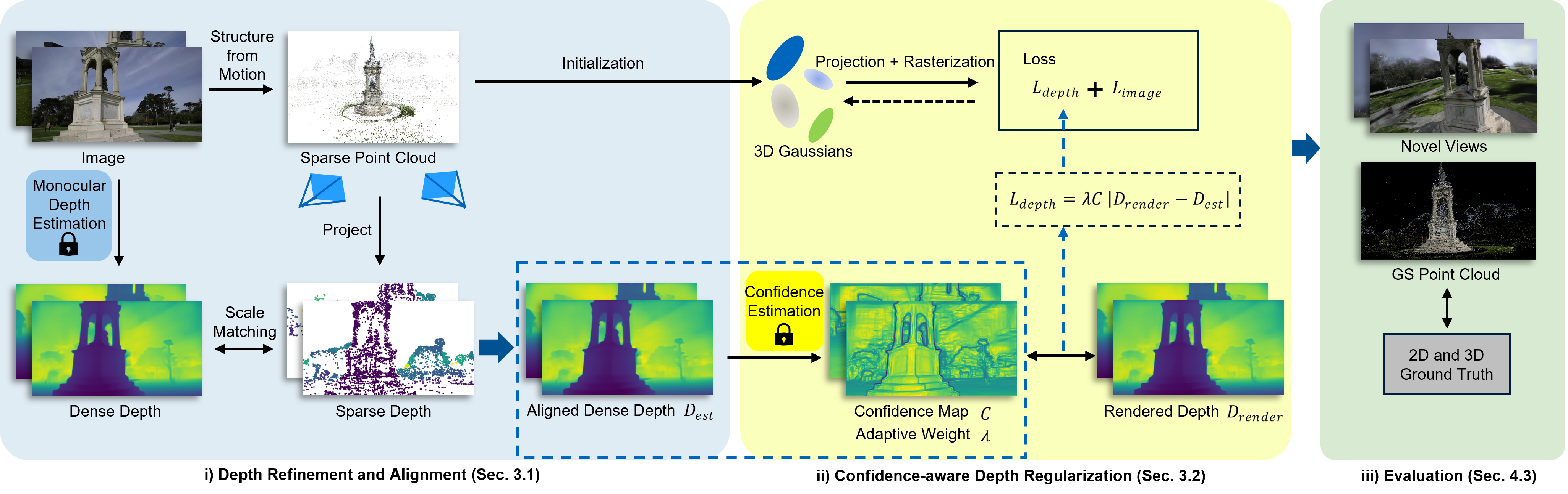
Figure 1: Overview of our confidence-aware depth regularization framework for 3DGS. Our method introduces three key components: i) depth refinement and alignment, ii) confidence-aware depth regularization through multi-cue feature analysis, and
iii) comprehensive 2D and 3D evaluation metrics for assessing both rendering quality and geometric accuracy. This framework enables stable optimization and improved reconstruction results.

In summary, the main contributions of this work are as follows:

• We propose a depth refinement and alignment method that aligns monocular depth estimates with sparse depth data from SfM through gradient descent optimization, improving geometric consistency across multiple views.

• We introduce a confidence-aware depth regularization term that generates confidence maps by analyzing features from both depth maps and RGB images, and adaptively adjusts depth loss weights to achieve stable optimization.

• We present comprehensive 2D and 3D evaluations on benchmark datasets, providing systematic comparisons with state-of-the-art 3DGS variants and detailed analysis of optimization behavior in both NVS and geometric reconstruction.

2 Related Work

In this section, we first introduce the development of NVS techniques from traditional geometric approaches to recent neural rendering methods. We then discuss the integration of depth information in 3DGS and various depth-based optimization strategies. Finally, we describe the fundamental formulation of 3DGS that serves as the basis for our method.

Novel View Synthesis. NVS aims to generate novel views of a scene from unseen perspectives. It commonly relies on 3D reconstruction techniques to capture spatial structures and preserve visual details. A fundamental step in NVS involves estimating the camera’s intrinsic and extrinsic parameters (Mueller et al.,, 2019), a task typically performed using Structure-from-Motion (SfM) methods (Ullman,, 1979). These methods leverage feature matching across multiple views and epipolar geometry to recover both camera poses and sparse 3D scene structure. Building upon SfM results, Multi-view Stereo (MVS) techniques (Tomasi and Kanade,, 1992) can further enhance the reconstruction by creating denser 3D models.

Beyond traditional methods such as SfM and MVS, deep learning has brought new advances to NVS, particularly with NeRF. NeRF represents scenes as continuous volumetric radiance fields encoded by a neural network (Mildenhall et al.,, 2021). It achieves photorealistic rendering by modeling the color and density of each 3D point based on the viewing direction. Despite its success in generating high-quality novel views, NeRF’s computational demands often limit its efficiency in real-time applications. To meet the demand for faster rendering, 3DGS has emerged as a promising alternative. It offers an efficient approach by using $\alpha$-blending rasterization rather than the computationally intensive volume rendering. By optimizing the spatial distribution, scales, rotations, and opacities of the Gaussian primitives, 3DGS achieves both real-time rendering and high-quality reconstruction (Chung et al.,, 2024).

Gaussian Splatting with Depth Information. Recent works have explored integrating monocular depth estimation into 3DGS optimization. Various depth estimation models have been employed, such as DPT (Ranftl et al.,, 2021), which has been applied in Chung et al., (2024) and Turkulainen et al., (2024), and ZoeDepth (Bhat et al.,, 2023), which has been utilized in Li et al., (2024) and Zhu et al., (2023). Recent advances in monocular depth estimation have led to new models such as Depth Anything V2 (Yang et al.,, 2024). In this work, we investigate the integration of this recent depth estimation model into 3DGS optimization.

Many existing methods adopt the depth-based regularization framework introduced by Chung et al., (2024), which extends the original 3DGS rasterization pipeline to produce rendered depth maps for geometric supervision. Expanding on this framework, researchers have proposed strategies to enhance 3DGS performance, such as achieving comparable NVS quality with fewer training images (Zhu et al.,, 2023) and improving rendering details (Li et al.,, 2024). In terms of depth regularization, different approaches have been explored, including fixed-weight balancing between depth and image losses (Liu et al.,, 2024), segmented depth regularization with varying emphases (Li et al.,, 2024), and early stopping strategies based on depth loss variations (Chung et al.,, 2024). However, these approaches rely on the estimated depth values without explicitly considering their reliability, which may lead to inconsistent optimization behavior across different scenes. Furthermore, while existing methods have demonstrated improvements in 2D image synthesis quality, there has been limited systematic analysis of how depth information affects the 3D geometric accuracy. To tackle these limitations, our method proposes a confidence-aware depth regularization strategy that selectively incorporates depth supervision based on multi-cue reliability assessment, aiming to achieve more stable optimization in both novel view synthesis and geometric reconstruction tasks.

3D Gaussian Splatting Formulation. 3DGS represents 3D scenes using a collection of 3D Gaussian primitives. Each primitive is parameterized by its center $\mu\in\mathbb{R}^{3}$, scale $s\in\mathbb{R}^{3}$, rotation (quaternion) $q\in\mathbb{R}^{4}$, opacity $\alpha\in\mathbb{R}$, and color features $f\in\mathbb{R}^{K}$. The complete parameter set for the $i$-th Gaussian is denoted as $\theta_{i}=\{\mu_{i},s_{i},q_{i},\alpha_{i},f_{i}\}$ (Kerbl et al.,, 2023). The Gaussian function is expressed as:

$$G_{i}(x)=\exp\left(-\frac{1}{2}(x-\mu_{i})^{T}\Sigma_{i}^{-1}(x-\mu_{i})\right),$$ (1)

where the covariance matrix $\Sigma$ is determined by scale $s$ and rotation $q$.

For rendering, 3DGS employs an efficient rasterization pipeline that performs $\alpha$-blending of projected Gaussians. The color $C$ of each pixel is computed by blending contributions from $N$ overlapping Gaussians:

$$C=\sum_{j\in N}c_{j}\alpha_{j}T_{j},$$ (2)

where $T_{j}=\prod_{k=1}^{j-1}(1-\alpha_{k})$ represents the accumulated transparency. Here, $c_{j}$ and $\alpha_{j}$ denote the color and opacity of the $j$-th Gaussian, respectively. This formulation naturally handles occlusion by giving priority to Gaussians closer to the camera.

The depth value $D$ for each pixel is computed through normalized $\alpha$-weighted averaging:

$$D=\frac{\sum_{j\in N}d_{j}\alpha_{j}T_{j}}{\sum_{j\in N}\alpha_{j}T_{j}},$$ (3)

where $d_{j}=(R_{i}p_{j}+T_{i})_{z}$ represents the depth of the $j$-th Gaussian relative to the $i$-th camera. This normalization ensures robust depth estimation even in regions with sparse Gaussian coverage (Chung et al.,, 2024).

3 Methodology

In this section, we present our methodology for enhancing 3DGS through two key components: i) depth refinement and alignment, and ii) confidence-aware depth regularization. The proposed method integrates depth information into the optimization process by considering its reliability and adaptively adjusting its influence during training.

3.1 Depth Refinement and Alignment

To obtain reliable depth information for regularization, we propose a two-stage process: initial depth estimation and subsequent depth refinement through alignment with sparse geometric constraints.

Given an input image $I\in\mathbb{R}^{H\times W\times 3}$, we first obtain an initial depth map $D_{init}\in\mathbb{R}^{H\times W}$ using a pre-trained monocular depth estimation model $f$:

$$D_{init}=f(I)$$ (4)

where $f$ represents depth estimation models, for example, ZoeDepth (Bhat et al.,, 2023) or Depth Anything V2 (Yang et al.,, 2024).

To provide geometric constraints for depth refinement, we generate a target depth map $D_{target}$ by projecting the sparse point cloud obtained from SfM. For each 3D point $P\in\mathbb{R}^{3}$, its projected depth value at pixel coordinate $p$ is computed as:

$$D_{target}(p)=[K(RP+T)]_{z}$$ (5)

where $K\in\mathbb{R}^{3\times 3}$ is the camera intrinsic matrix, $R\in\mathbb{R}^{3\times 3}$ and $T\in\mathbb{R}^{3}$ are the camera extrinsic parameters, and $[\cdot]_{z}$ denotes the z-component of the projected point.

Following Chung et al., (2024), we refine the initial depth estimates by aligning them with the sparse point cloud data through an optimization process. The objective function is formulated as:

$$\min_{\alpha,\beta}\sum_{p\in\Omega}w(p)(D_{target}(p)-(\alpha D_{init}(p)+\beta))^{2}+\lambda R(\alpha D_{init}+\beta)$$ (6)

where:

• $\Omega$ denotes the set of pixels with valid point cloud projections

• $w(p)$ weights each pixel based on its point cloud reprojection error

• $\alpha$ and $\beta$ are scale and shift parameters for depth alignment

• $\lambda$ balances the alignment term and regularization term

The regularization term $R(\cdot)$ ensures physical validity by penalizing negative depth values:

$$R(D)=\sum_{p}\max(0,-D(p))^{2}$$ (7)

We solve this optimization problem using gradient descent to obtain the optimal scale and shift parameters. During the optimization, we compute the alignment loss $l_{a}$ as the weighted mean squared error between the transformed and target depth:

$$l_{a}=\frac{1}{|\Omega|}\sum_{p\in\Omega}w(p)(D_{target}(p)-D_{trans}(p))^{2}$$ (8)

where $D_{trans}(p)=\alpha D_{init}(p)+\beta$ represents the transformed initial depth using the current scale and shift parameters. This alignment loss not only guides the optimization process but also serves as an important indicator of depth estimation reliability, which is utilized in our subsequent confidence-aware depth regularization.

The refined depth map provides geometric constraints for the following optimization process, while the alignment loss $l_{a}$ offers valuable information about the overall quality of depth estimation and alignment, enabling adaptive adjustment of depth supervision in the next stage.

3.2 Confidence-aware Depth Regularization

Building upon the refined depth maps and alignment quality information obtained from the previous stage, we propose a confidence-aware regularization scheme that adaptively incorporates depth supervision into the 3DGS optimization process. Inspired by Wysocki et al., (2023), our approach combines local depth reliability assessment with global alignment quality to guide the optimization.

We evaluate the reliability of depth values through a confidence map $C$ that integrates multiple complementary features:

$$C=w_{e}C_{e}+w_{t}C_{t}+w_{g}C_{g}$$ (9)

where:

• $C_{e}$ captures edge-aware confidence using Canny edge detection:

  $$C_{e}=1-\frac{E(I)}{255}$$ (10)

  where $E(I)$ represents the edge map of image $I$

• $C_{t}$ measures texture reliability using the Laplacian operator:

  $$C_{t}=1-\frac{|\nabla^{2}I|}{\max(|\nabla^{2}I|)}$$ (11)

• $C_{g}$ evaluates depth consistency through spatial gradients:

  $$C_{g}=\frac{1}{|\nabla D|+\epsilon}$$ (12)

  where $\nabla D$ represents the spatial gradients of the refined depth map, and $\epsilon$ is a small constant to prevent numerical instability

The weights are chosen to emphasize texture reliability while maintaining balanced contributions from edge and gradient features, with $w_{t}>w_{g}>w_{e}$.

Based on the confidence map, we formulate the depth supervision term as:

$$\mathcal{L}_{depth}=\frac{1}{|\Omega|}\sum_{p\in\Omega}C(p)|D_{render}(p)-D_{est}(p)|$$ (13)

where $\Omega$ denotes the set of valid depth pixels, $D_{render}(p)$ is the rendered depth from the current 3DGS model, and $D_{est}(p)$ is the refined depth value from our alignment stage. The confidence map $C(p)$ ensures that the supervision focuses on reliable depth regions.

To adaptively balance the depth supervision, we introduce a weight term $\lambda_{d}(l_{a})$ based on the global alignment quality:

$$\lambda_{d}(l_{a})=\lambda_{max}e^{-kl_{a}}$$ (14)

where $\lambda_{max}$ controls the maximum influence of depth supervision, and $k$ determines how quickly the weight decreases with increasing alignment loss $l_{a}$. This exponential form ensures that depth supervision is stronger when the alignment quality is better (lower $l_{a}$).

For image reconstruction, we follow the original 3DGS formulation:

$$\begin{split}\mathcal{L}_{image}=&(1-\lambda_{dssim})\|I_{pred}-I_{gt}\|_{1}\\ &+\lambda_{dssim}(1-SSIM(I_{pred},I_{gt}))\end{split}$$ (15)

where $\lambda_{dssim}$ balances the contribution of L1 loss and structural similarity.

Our final optimization objective combines image reconstruction with confidence-aware depth supervision:

$$\mathcal{L}=\mathcal{L}_{image}+\lambda_{d}(l_{a})\mathcal{L}_{depth}$$ (16)

This confidence-aware regularization scheme effectively integrates depth information by considering both pixel-wise depth reliability and global alignment quality. The local confidence weighting helps focus the supervision on reliable regions, while the adaptive global weight automatically adjusts the strength of depth supervision based on the overall alignment quality, and leads to more stable optimization behavior.

4 Experiments

We conducted comprehensive experiments to evaluate the effectiveness of our proposed CDGS method. Our evaluation framework encompassed both novel view synthesis quality and geometric reconstruction accuracy through extensive comparisons with state-of-the-art methods. This section first describes the experimental setup, including datasets and implementation details, followed by detailed qualitative and quantitative analyses.

4.1 Datasets

We evaluated our method on the Tanks and Temples (TnT) benchmark dataset (Knapitsch et al.,, 2017), which provides multi-view images and high-precision laser-scanned ground truth geometry. The selected scenes included complex outdoor environments (Barn, Truck, Caterpillar, Ignatius) and detailed indoor scenarios (Meeting Room, Church), which featured diverse geometric complexities and lighting conditions (Urban and Jutzi,, 2017). Following the protocol established by Chung et al., (2024), we employed a random sampling strategy where each captured view was assigned to either the training or testing set with equal probability. This probabilistic split strategy ensured a balanced distribution between training and testing data while maintaining well-distributed testing views across different viewpoints.

Our evaluation framework incorporated both 2D and 3D metrics to provide a comprehensive assessment of the method’s performance. For 2D novel view synthesis quality, we utilized three complementary metrics: PSNR for pixel-wise reconstruction accuracy, SSIM for structural similarity assessment, and LPIPS for perceptual quality evaluation. The 3D geometric accuracy assessment combined the official evaluation protocol of Tanks and Temples (Knapitsch et al.,, 2017) with the M3C2 distance metric (Lague et al.,, 2013). First, following the official evaluation protocol of Tanks and Temples, we performed a systematic point cloud registration process between the reconstructed geometry and ground truth, followed by the computation of precision and recall metrics. The protocol included F-score calculations at multiple distance thresholds to quantify the reconstruction quality across different levels of geometric detail. Additionally, inspired by Jäger et al., (2024), we utilized the M3C2 distance metric to provide a more detailed analysis of the geometric accuracy. This metric enabled a precise measurement of the local distances between the reconstructed and ground truth surfaces, offering insights into the fine-scale geometric fidelity of our reconstruction results.

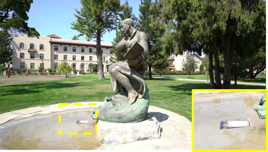
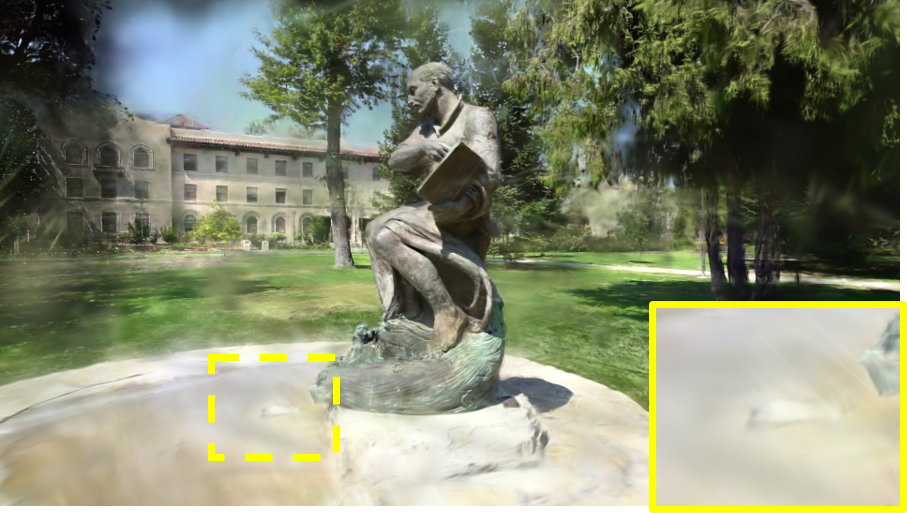
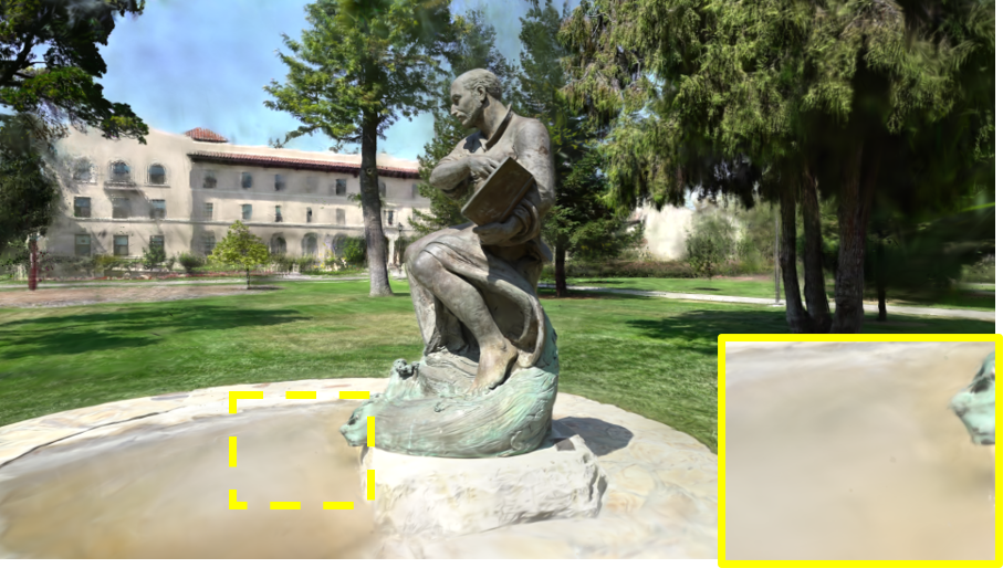
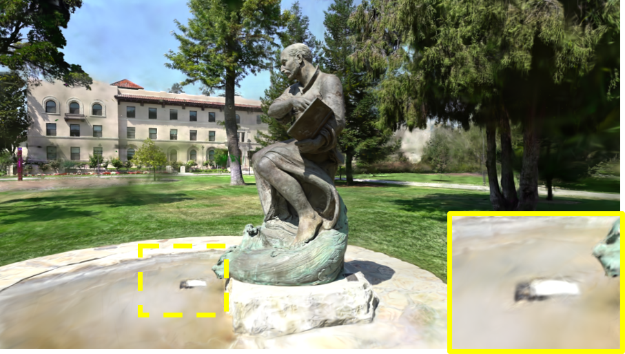
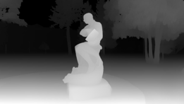
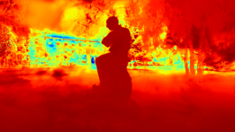
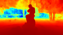
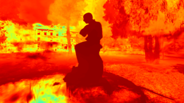
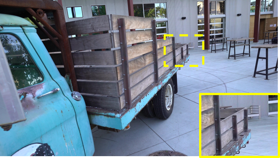
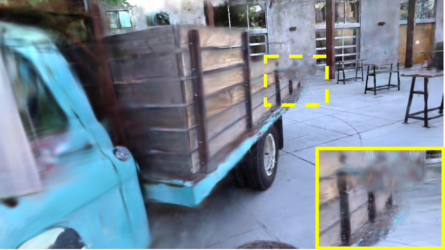
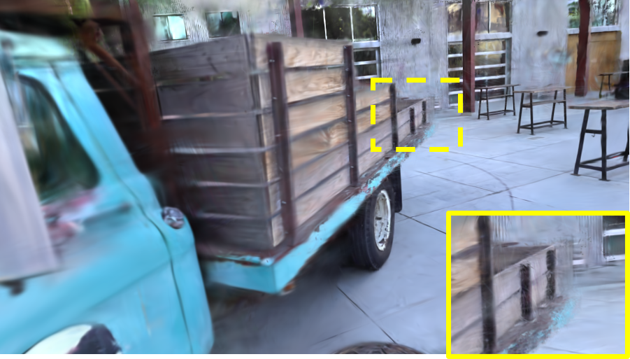
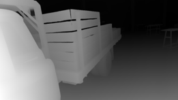
Ground Truth

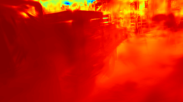
3DGS

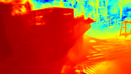
DRGS

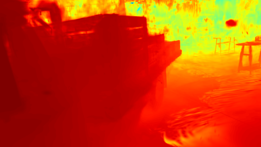
CDGS (Ours)

Figure 2: Qualitative comparison of NVS results on the Ignatius (top two rows) and Truck (bottom two rows) scenes at iteration 9,000. For each scene: rows 1&3 show synthesized RGB images, rows 2&4 present corresponding depth maps. Reference depth maps are generated using Depth Anything V2, and comparison depth maps are rendered from respective 3D representations. Applying our method required an additional preprocessing time of 1.5 seconds per image on average, ensuring its uniform applicability across all inputs. Yellow boxes highlight regions where our method better preserves geometric and radiometric details.

4.2 Implementation details

Our implementation was built upon the official codebase of 3DGS (Kerbl et al.,, 2023), and incorporated the depth-aware rasterization pipeline from DRGS (Chung et al.,, 2024). We implemented our method using PyTorch and trained all models on a single NVIDIA Tesla V100-PCIE-32GB GPU. For depth estimation, we primarily used Depth Anything V2 (Yang et al.,, 2024), while also supporting ZoeDepth (Bhat et al.,, 2023) as an alternative monocular depth estimator. Following Chung et al., (2024), for depth alignment optimization, we employed Adam optimizer with an initial learning rate of 1.0 and an exponential decay schedule, with settings of outlier pruning ratio ($1\times 10^{-3}$) and convergence threshold ($1\times 10^{-5}$). For all experiments, we maintained the original optimization parameters and training pipeline from Kerbl et al., (2023) and trained for 30,000 iterations for fair comparison. For baseline comparison, we disabled the early stopping mechanism in DRGS (Chung et al.,, 2024) which typically terminates training before 2,000 iterations, to ensure a fair evaluation of its full potential. The key parameters specific to our method were the confidence map weights ($w_{t}=0.5$, $w_{g}=0.3$, and $w_{e}=0.2$) and depth loss adaptation parameters ($\lambda_{max}=0.6$ and $k=150$). The depth alignment process and the generation of confidence maps took approximately 1.5 seconds per image. The whole training process took approximately 2 hours per scene on our hardware configuration.

4.3 Results

We evaluated our method with two leading baselines: the original 3DGS (Kerbl et al.,, 2023) and DRGS (Chung et al.,, 2024). Our evaluation focused on both 2D novel view synthesis quality and 3D geometry reconstruction accuracy.

Novel View Synthesis Quality. We assessed the effectiveness of our method in NVS through both qualitative and quantitative analyses, with particular attention to early-stage performance. Our method demonstrated consistent advantages throughout the first half of training iterations, and we showcase the results at iteration 9,000 (30% of total iterations) as a representative example. Figure 2 provides detailed visual comparisons on two representative scenes (Ignatius and Truck) at this stage. The comparison presented both synthesized RGB images and their corresponding depth maps to demonstrate the overall reconstruction quality. Our method exhibited notably better geometric detail preservation during these early stages, especially evident in the highlighted regions (yellow boxes), and suggested more efficient optimization and faster convergence to high-quality reconstructions.

For quantitative evaluation, Table 1 presents 2D evaluation metrics across different scenes at iteration 9,000. At this early stage, compared to the original 3DGS, our method showed improvements with PSNR gains of up to 2.815 dB in Barn scene and SSIM improvements of up to 0.050 in Caterpillar scene. Besides, our method demonstrated competitive results with DRGS in terms of average SSIM (0.600) and LPIPS (0.459).

Table 1: Quantitative comparison of novel view synthesis quality on the TnT dataset. The metrics include PSNR (dB), SSIM, and LPIPS. $\uparrow$ indicates higher is better, $\downarrow$ indicates lower is better. Best results are highlighted in green and shown in bold.

Scene	3DGS			DRGS			Ours
	PSNR$\uparrow$	SSIM$\uparrow$	LPIPS$\downarrow$	PSNR$\uparrow$	SSIM$\uparrow$	LPIPS$\downarrow$	PSNR$\uparrow$	SSIM$\uparrow$	LPIPS$\downarrow$
Barn	17.212	0.588	0.545	19.987	0.633	0.463	20.027	0.638	0.461
Caterpillar	16.061	0.587	0.558	18.698	0.553	0.456	18.836	0.567	0.452
Truck	13.933	0.546	0.587	15.291	0.574	0.492	15.132	0.578	0.495
Ignatius	16.142	0.452	0.537	17.918	0.502	0.466	17.813	0.510	0.452
Meeting Room	16.938	0.677	0.508	19.746	0.727	0.401	18.058	0.698	0.417
Church	15.619	0.568	0.555	17.098	0.612	0.479	16.916	0.609	0.474
Average	15.984	0.570	0.548	18.123	0.600	0.460	17.797	0.600	0.459

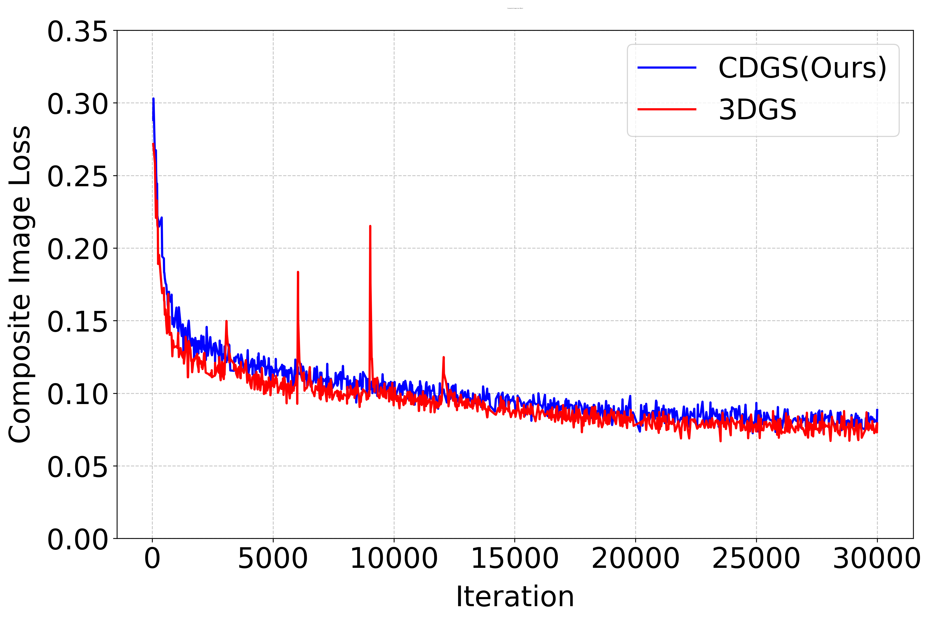
Barn

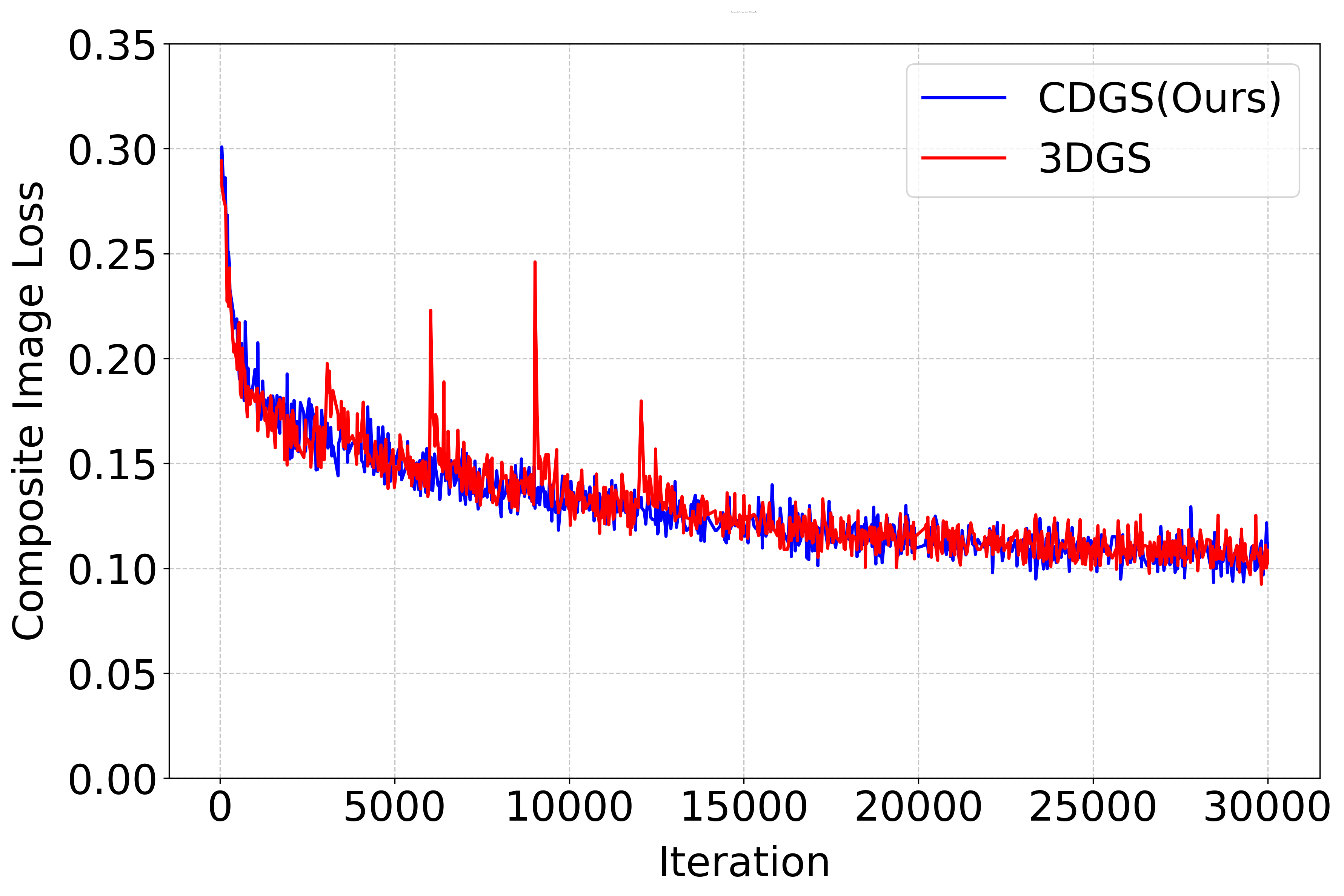
Caterpillar

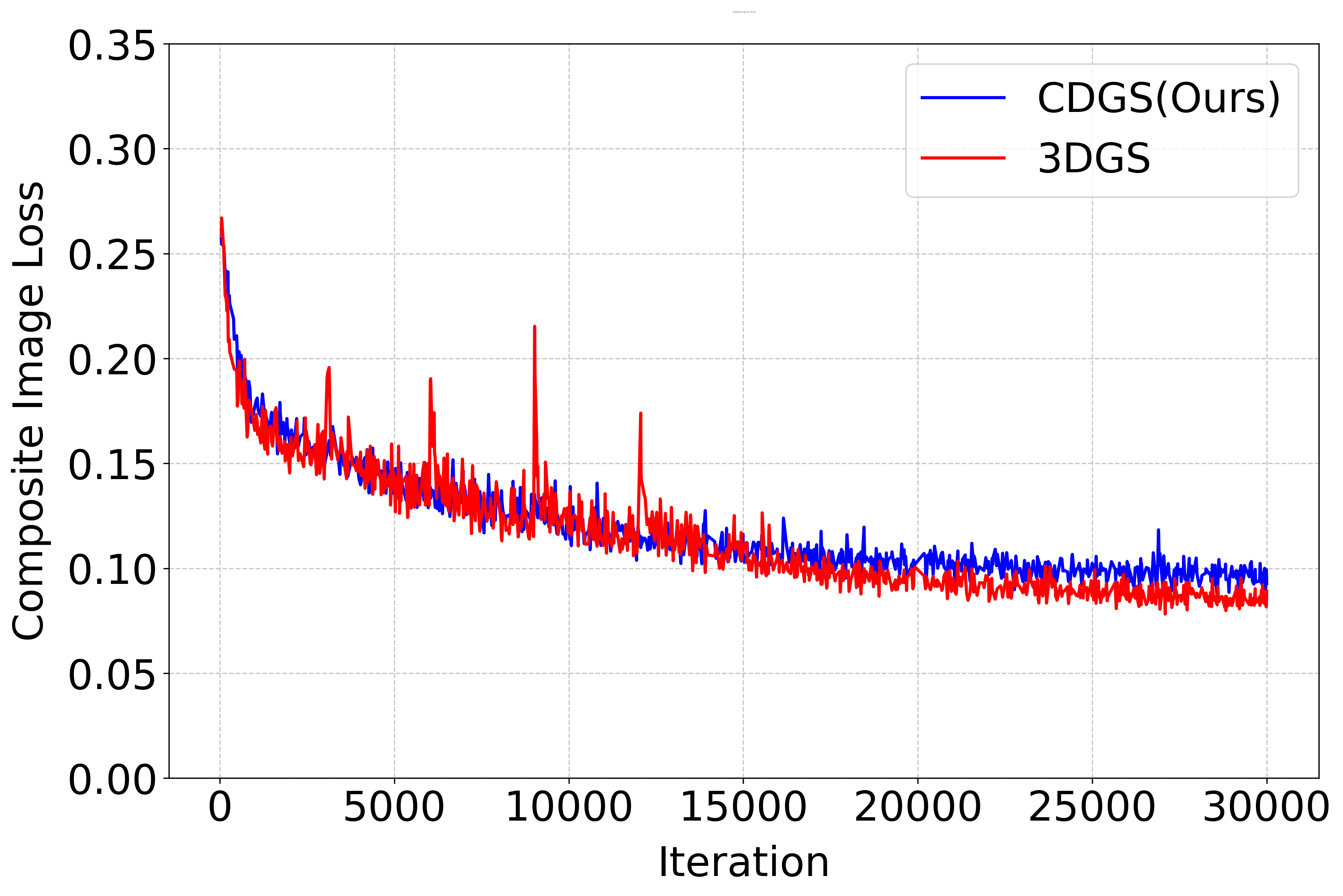
Truck

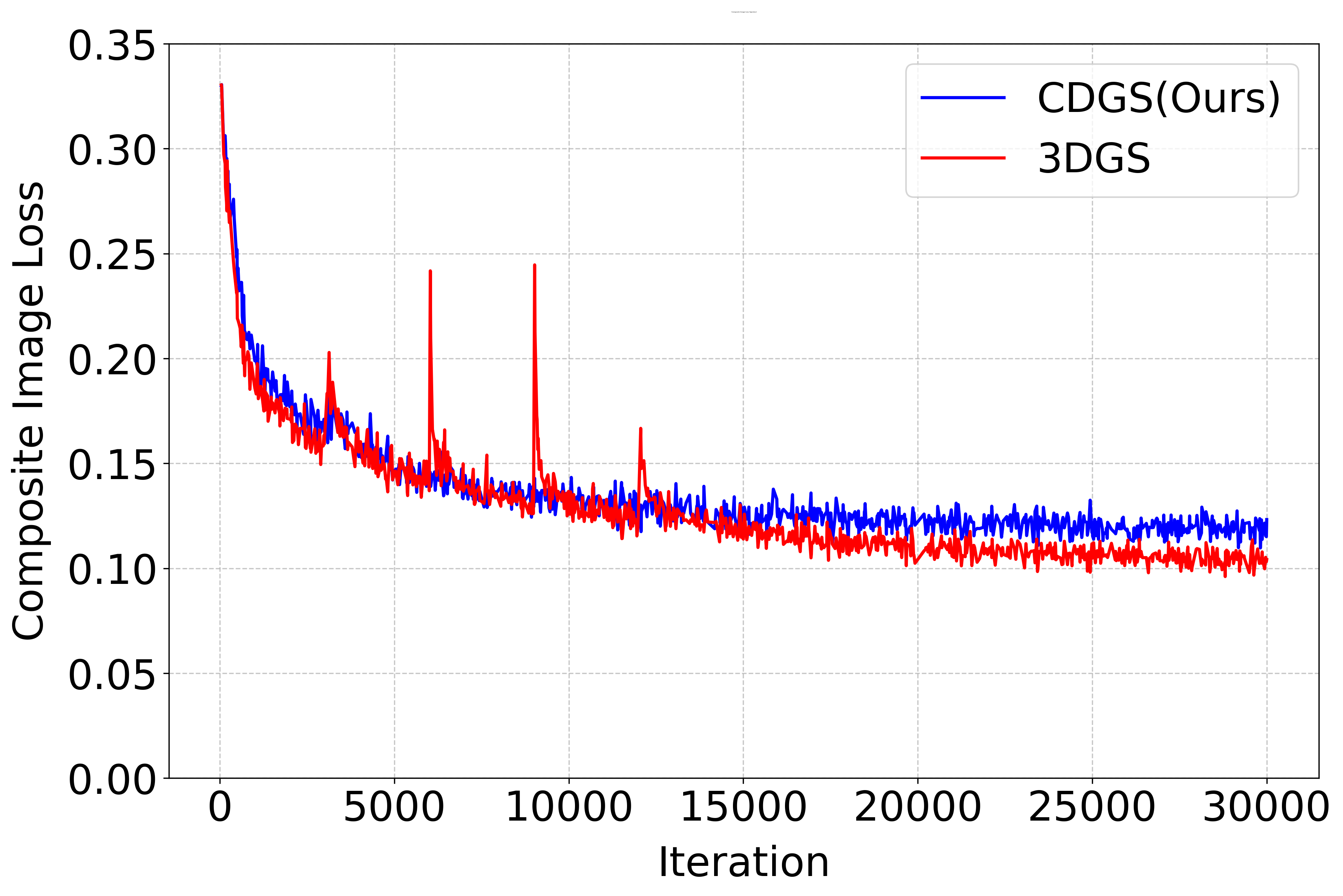
Ignatius

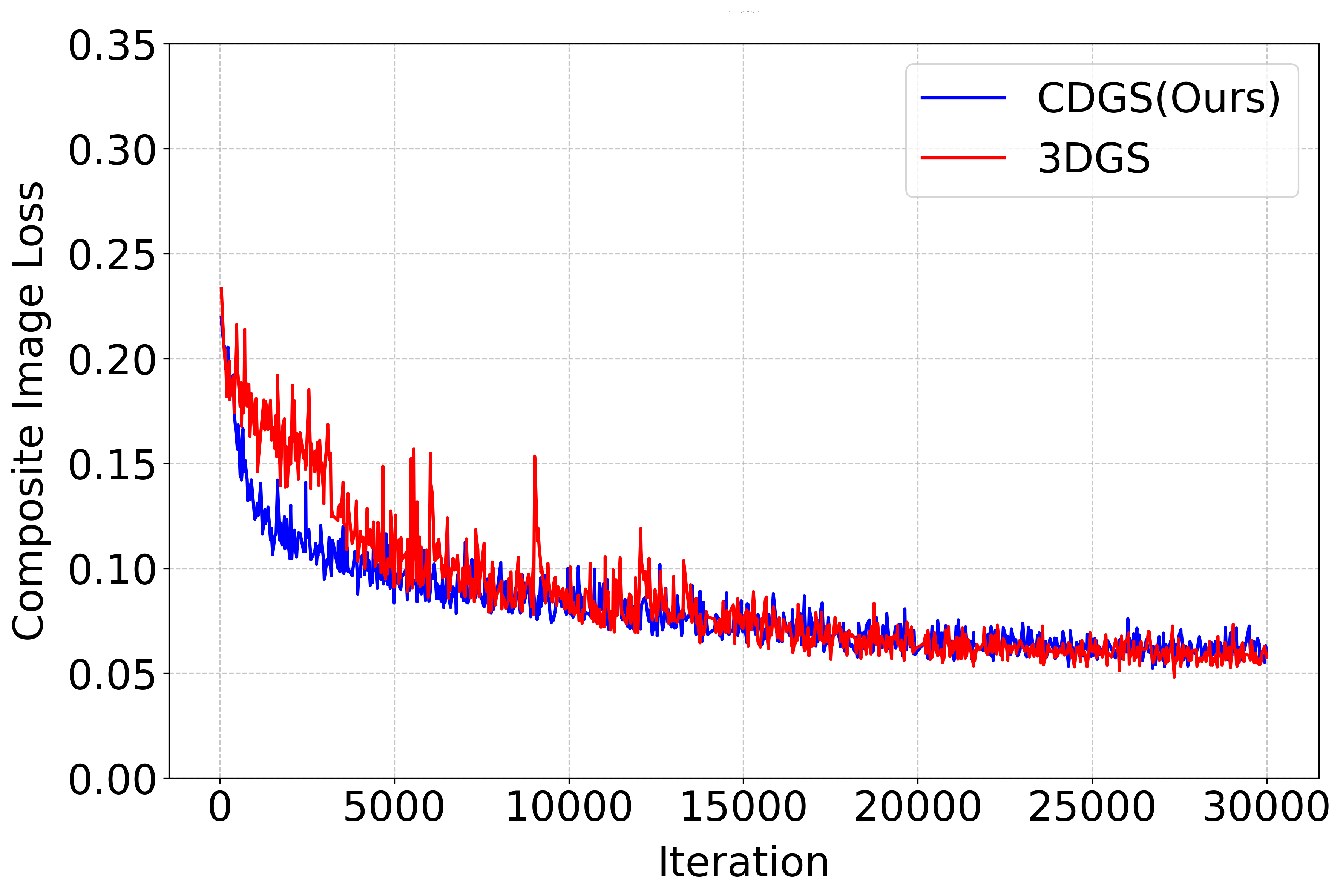
Meetingroom

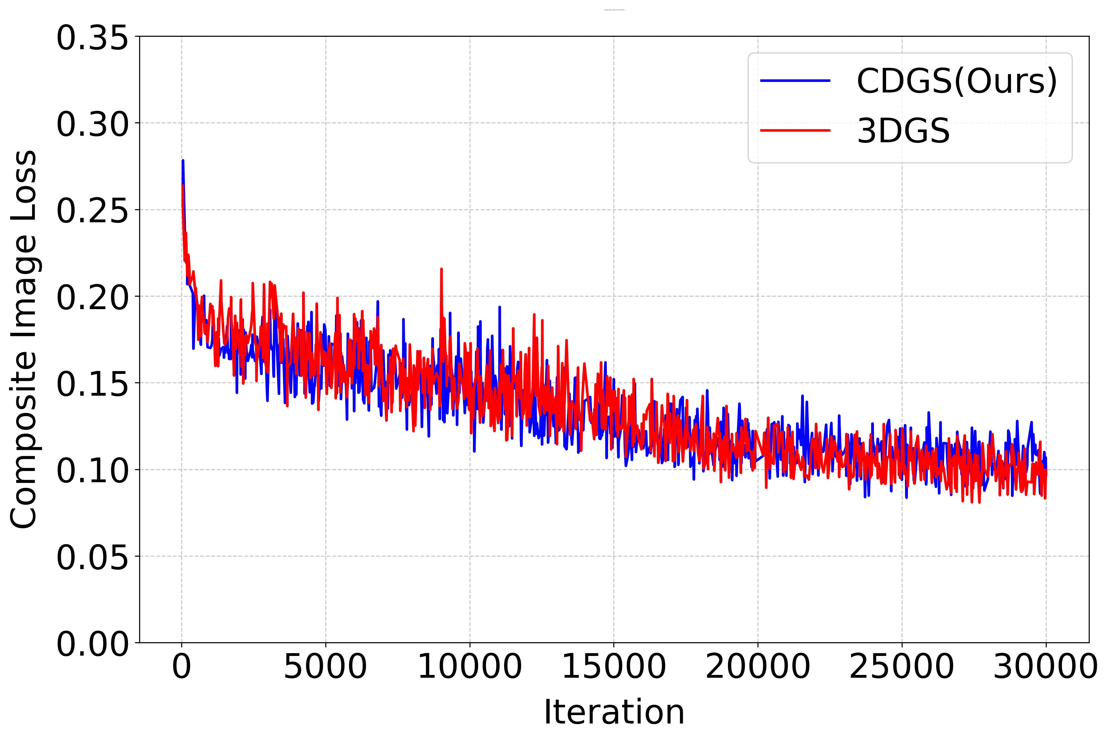
Church

Figure 3: Comparison of composite image loss during training across different scenes from the TnT dataset. Each plot shows the convergence behavior over 30,000 iterations, with our method (blue) and 3DGS (red). Lower values indicate better performance.

Training Stability and Convergence. Figure 3 illustrates the convergence behavior of the composite image loss during training across different scenes. The composite image loss combines L1 reconstruction loss and SSIM-based perceptual loss, providing a comprehensive measure of image synthesis quality. Our approach demonstrated more stable convergence patterns compared to the original 3DGS, with fewer fluctuations across all tested scenes.

Geometric Accuracy. We evaluated the geometric accuracy through three complementary metrics: F-score evolution, geometric completeness, and M3C2 distance analysis. Figure 4 illustrates the F-score evolution during training for three representative scenes (Barn, Caterpillar, and Meeting Room). The results showed that both depth-aware methods (DRGS and CDGS) achieved higher F-scores compared to the original 3DGS across these scenes.

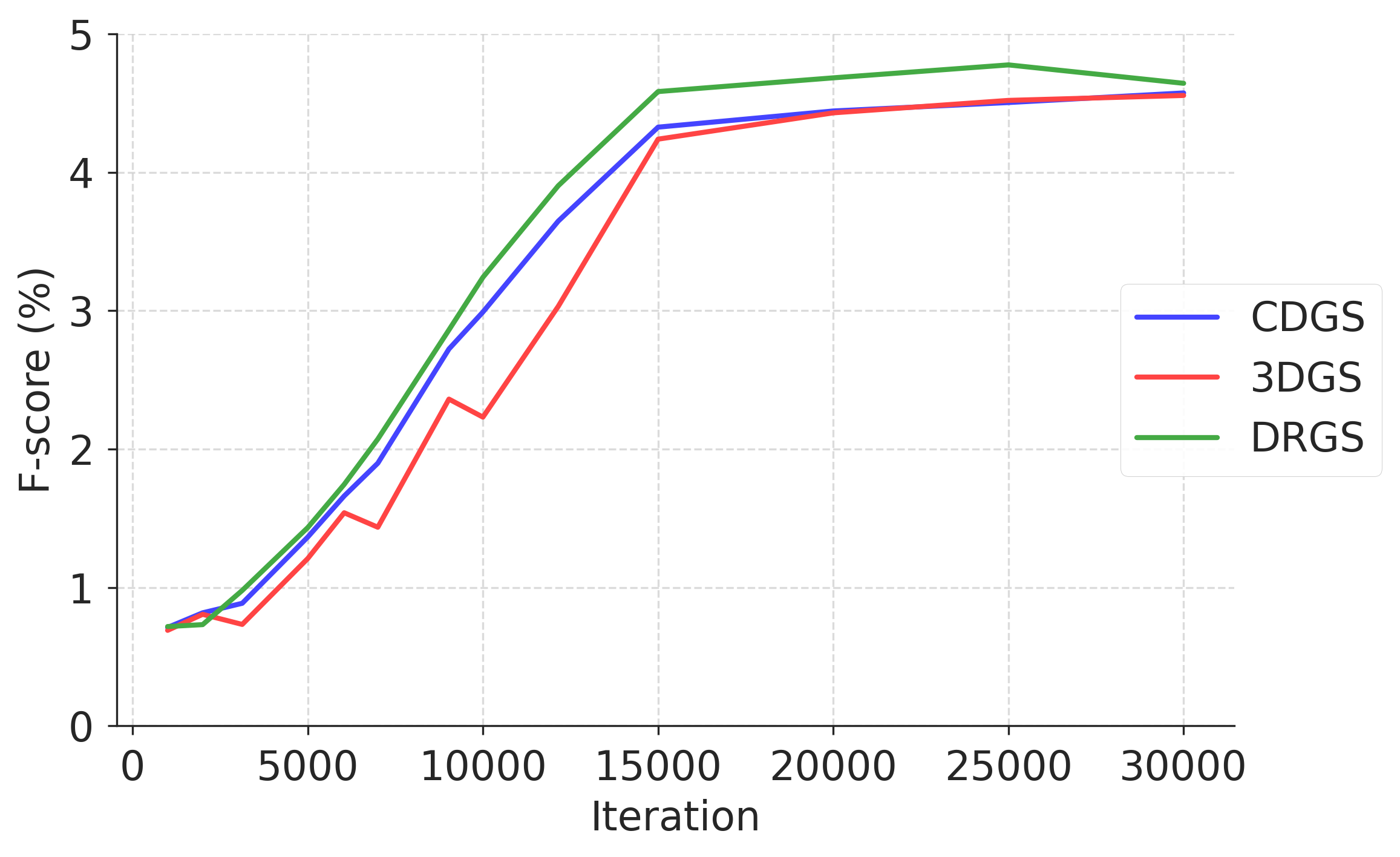
Barn

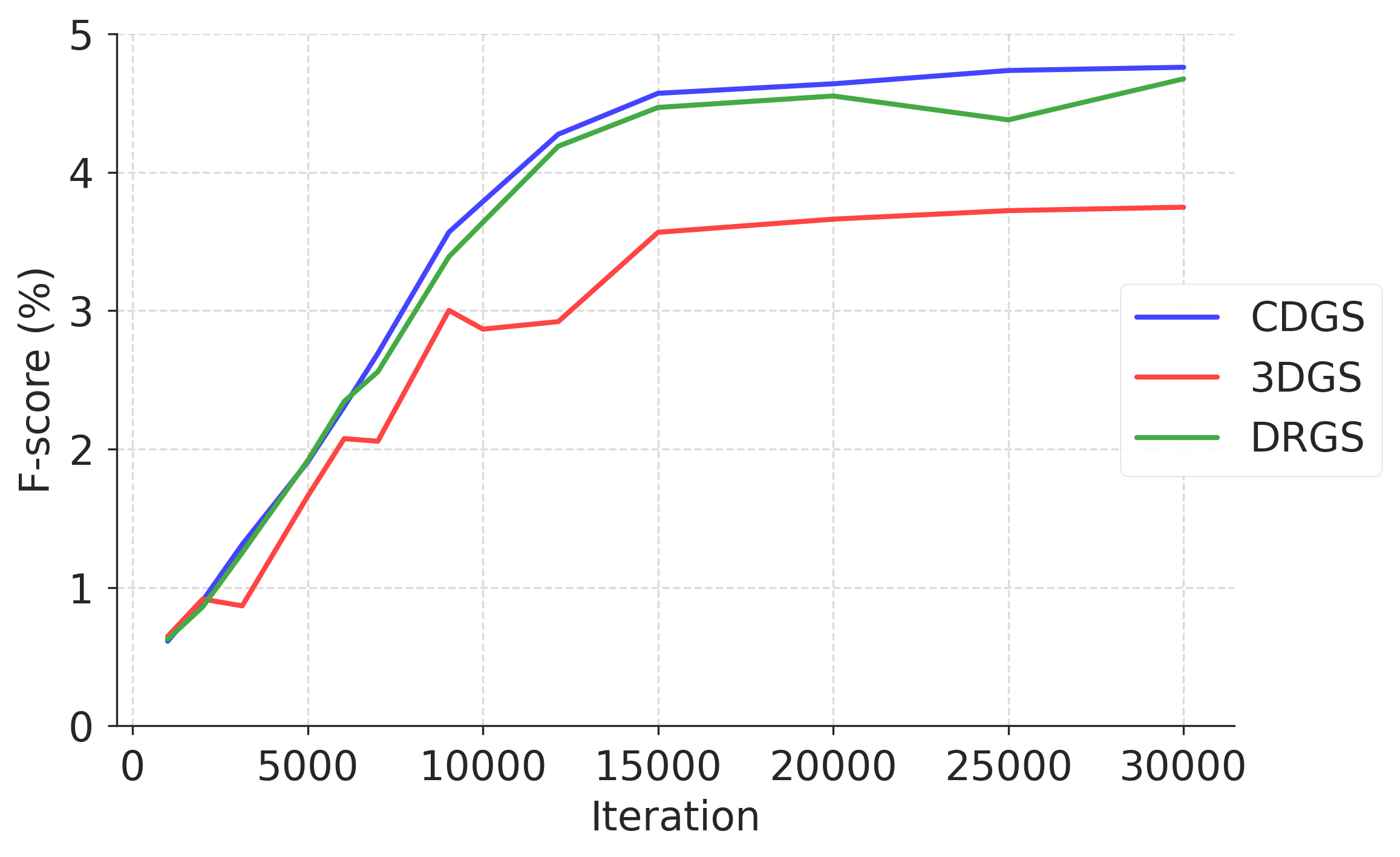
Caterpillar

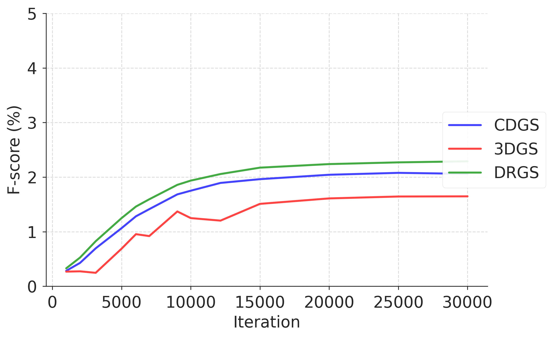
Meetingroom

Figure 4: F-score evolution during training for Barn, Caterpillar, and Meeting Room scenes from the TnT dataset. Our method (CDGS, in blue), DRGS (in green), and 3DGS (in red). The y-axis range is set to 0-5%.

For a comprehensive evaluation at iteration 15,000 (where most scenes demonstrate stable performance), Table 2 presents the geometric completeness results. While the original 3DGS achieves higher precision values across all scenes (with the highest being 0.248 in Ignatius), both depth-aware methods show better recall and F-score performance.

Table 2: Geometric completeness comparison at iteration 15,000. F-score values are in percentage (%). Best results are shown in bold.

Scene	3DGS				DRGS				CDGS (Ours)
	Precision	Recall	F-score(%)		Precision	Recall	F-score(%)		Precision	Recall	F-score(%)
Barn	0.143	0.025	4.2		0.105	0.029	4.5		0.099	0.028	4.4
Caterpillar	0.113	0.021	3.5		0.102	0.028	4.4		0.106	0.029	4.5
Truck	0.039	0.006	1.1		0.031	0.006	1.0		0.033	0.007	1.2
Ignatius	0.248	0.072	11.3		0.160	0.033	5.4		0.166	0.033	5.4
Meetingroom	0.078	0.008	1.5		0.067	0.013	2.2		0.067	0.011	1.9
Church	0.061	0.006	1.1		0.052	0.011	1.9		0.054	0.013	2.1
Average	0.114	0.023	3.8		0.086	0.020	3.2		0.088	0.020	3.3

Following Jäger et al., (2024), we further employed the M3C2 metric to evaluate point cloud accuracy (Table 3). Our method achieved the lowest RMSE values in five out of six scenes, with an average RMSE of 0.120 meters. Figure 5 provides a qualitative visualization of the M3C2 distance analysis on the Caterpillar scene. The color-coded visualization shows the signed distances between our reconstructed point cloud and the ground truth, where green indicates small distances, blue represents inward deviations, and red shows outward deviations. The predominant green coloring in our reconstruction demonstrates the high geometric fidelity achieved by our method, particularly in preserving the complex mechanical structures of the scene.

Table 3: Point cloud distance analysis using M3C2 metric. RMSE values are in meters. Lower values indicate better accuracy. Best results are shown in bold.

Scene	3DGS	DRGS	CDGS (Ours)
Barn	0.084	0.077	0.076
Caterpillar	0.082	0.081	0.080
Truck	0.201	0.199	0.195
Ignatius	0.032	0.035	0.035
Meetingroom	0.158	0.159	0.157
Church	0.187	0.178	0.177
Average	0.124	0.122	0.120

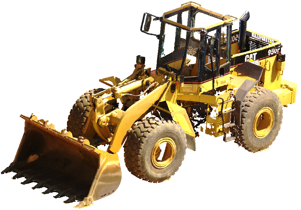
Ground truth point cloud

M3C2 distance visualization

Figure 5: M3C2 distance analysis visualization of our CDGS reconstruction on the Caterpillar scene. The color bar indicates the signed distances to the ground truth surface, where green represents small distances ($\pm$0.05 m), blue indicates negative deviations
(up to -0.4 m), and red shows positive deviations (up to 0.4 m).

Ablation Studies. We conducted ablation studies on the Ignatius scene to evaluate the contribution of each key component in our method (Table 4). Removing the confidence map mechanism led to performance degradation across all metrics at 30,000 iterations, with PSNR decreasing from 18.22 dB to 18.04 dB. Similarly, replacing our adaptive depth loss weighting scheme with fixed scale factors resulted in more substantial decreases, with PSNR dropping by 1.12 dB (from 18.22 dB to 17.10 dB) and SSIM declining from 0.519 to 0.484. At 15,000 iterations, our full method achieved a PSNR of 18.04 dB and LPIPS of 0.411, compared to 17.80 dB/0.424 without confidence map and 17.10 dB/0.458 with fixed depth loss.

Table 4: Ablation study results on the Ignatius scene at 30,000 iterations. Best results are shown in bold.

Method	PSNR$\uparrow$	SSIM$\uparrow$	LPIPS$\downarrow$
Ours (Full)	18.225	0.519	0.384
w/o Confidence Map	18.040	0.509	0.396
w/ Fixed Depth Loss	17.100	0.484	0.437

4.4 Discussion

The experimental results demonstrate the effectiveness of our method from multiple perspectives. For 2D novel view synthesis, our confidence-aware depth regularization enables better geometric detail preservation during early training stages (30% of total iterations) by effectively identifying and emphasizing reliable depth regions. While DRGS achieves slightly better average PSNR (18.12 dB vs. our 17.80 dB), our method shows particularly strong performance in scenes with complex geometric structures, such as the Barn (20.03 dB) and Caterpillar (18.84 dB) scenes, suggesting the effectiveness of our confidence-guided approach in handling challenging scenarios.

The geometric evaluation reflects a trade-off between precision and recall. The original 3DGS tends to generate more conservative but accurate reconstructions, achieving the highest precision across all scenes (e.g., 0.248 for Ignatius and 0.143 for Barn), while depth-aware methods achieve better geometric completeness through improved recall (e.g., increasing from 0.025 to 0.028 in Barn scene). This trade-off underscores the role of depth supervision in recovering more complete geometric structures. This is further supported by our M3C2 analysis, which shows that our method achieves the lowest RMSE values in five out of six scenes. On average, our approach achieves an RMSE of 0.120 meters, outperforming both 3DGS (0.124 meters) and DRGS (0.122 meters).

The convergence analysis demonstrates the stability benefits of depth-aware optimization. Both DRGS and our method achieve smoother convergence compared to the original 3DGS, with particularly stable behavior during 15-50% of total training iterations. This enhanced stability, combined with faster geometric convergence shown in F-score evolution (reaching F-scores of 4.4% for Barn and 4.5% for Caterpillar at iteration 15,000), makes our method particularly suitable for applications with training time constraints.

The ablation studies highlight two key aspects of our method. First, the confidence map mechanism, while yielding a modest improvement in final quality (PSNR increased from 18.04 dB to 18.22 dB), plays a critical role in establishing reliable geometric structures during early training. Second, replacing the adaptive depth loss weighting scheme with fixed weights significantly degrades performance, with PSNR dropping from 18.22 dB to 17.10 dB and SSIM decreasing from 0.519 to 0.484, emphasizing the importance of dynamic supervision.

Despite these improvements, our method has limitations. Performance varies across scenes, particularly in indoor environments with complex lighting (e.g., the Meeting Room scene shows a 1.69 dB lower PSNR than DRGS). Additionally, reconstructing fine geometric details remains challenging in occluded areas with limited depth information. These limitations suggest future research directions, including refined confidence estimation for challenging scenarios and exploration of additional geometric priors for improved reconstruction accuracy.

5 Conclusions

In this work, we have presented CDGS, a confidence-aware depth regularization framework for enhancing 3DGS. Through the integration of aligned monocular depth estimates and multi-feature confidence assessment, our method achieves more stable optimization and improved geometric reconstruction. The experimental results demonstrate that our approach effectively preserves geometric details during early training stages and maintains competitive performance in both 2D synthesis and 3D reconstruction tasks. We assume this work will encourage further research on leveraging depth information and geometric constraints to enhance the 3D reconstruction accuracy of Gaussian Splatting methods. Moreover, we expect this work will facilitate the development of efficient and accurate 3D reconstruction systems for real-world applications such as digital twin creation, heritage preservation, or forestry applications.

The ablation studies confirm the importance of confidence-aware depth supervision and adaptive loss weighting in achieving better optimization behavior. While showing promising results, our method still faces challenges in certain scenarios, particularly in indoor environments with complex lighting conditions and regions with intricate geometric structures. Future work will focus on advancing confidence estimation techniques to handle challenging scenes and exploring additional geometric priors to further improve reconstruction accuracy.

References

- Bhat et al., (2023) Bhat, S. F., Birkl, R., Wofk, D., Wonka, P., Müller, M., 2023. ZoeDepth: Zero-shot Transfer by Combining Relative and Metric Depth. arXiv preprint arXiv:2302.12288.
- Chung et al., (2024) Chung, J., Oh, J., Lee, K. M., 2024. Depth-regularized optimization for 3d gaussian splatting in few-shot images. Proceedings of the IEEE/CVF Conference on Computer Vision and Pattern Recognition, 811–820.
- Huang et al., (2024) Huang, B., Yu, Z., Chen, A., Geiger, A., Gao, S., 2024. 2d gaussian splatting for geometrically accurate radiance fields. ACM SIGGRAPH 2024 Conference Papers, 1–11.
- Jäger et al., (2024) Jäger, M., Kapler, T., Feßenbecker, M., Birkelbach, F., Hillemann, M., Jutzi, B., 2024. HoloGS: Instant Depth-based 3D Gaussian Splatting with Microsoft HoloLens 2. arXiv preprint arXiv:2405.02005.
- Kerbl et al., (2023) Kerbl, B., Kopanas, G., Leimkühler, T., Drettakis, G., 2023. 3D Gaussian Splatting for Real-Time Radiance Field Rendering. ACM Trans. Graph., 42(4), 139–1.
- Knapitsch et al., (2017) Knapitsch, A., Park, J., Zhou, Q.-Y., Koltun, V., 2017. Tanks and Temples: Benchmarking Large-scale Scene Reconstruction. ACM Transactions on Graphics (ToG), 36(4), 1–13.
- Lague et al., (2013) Lague, D., Brodu, N., Leroux, J., 2013. Accurate 3D Comparison of Complex Topography with Terrestrial Laser Scanner: Application to the Rangitikei Canyon (NZ). ISPRS Journal of Photogrammetry and Remote Sensing, 82, 10–26.
- Li et al., (2024) Li, J., Zhang, J., Bai, X., Zheng, J., Ning, X., Zhou, J., Gu, L., 2024. Dngaussian: Optimizing sparse-view 3d gaussian radiance fields with global-local depth normalization. Proceedings of the IEEE/CVF Conference on Computer Vision and Pattern Recognition, 20775–20785.
- Liu et al., (2024) Liu, Y., Li, C., Yang, C., Yuan, Y., 2024. EndoGaussian: Real-time Gaussian Splatting for Dynamic Endoscopic Scene Reconstruction. arXiv preprint arXiv:2401.12561.
- Mildenhall et al., (2021) Mildenhall, B., Srinivasan, P. P., Tancik, M., Barron, J. T., Ramamoorthi, R., Ng, R., 2021. NeRF: Representing Scenes as Neural Radiance Fields for View Synthesis. Communications of the ACM, 65(1), 99–106.
- Mueller et al., (2019) Mueller, M. S., Sattler, T., Pollefeys, M., Jutzi, B., 2019. Image-to-Image Translation for Enhanced Feature Matching, Image Retrieval and Visual Localization. ISPRS Annals of the Photogrammetry, Remote Sensing and Spatial Information Sciences, 4, 111–119.
- Petrovska and Jutzi, (2024) Petrovska, I., Jutzi, B., 2024. Vision through Obstacles: 3D Geometric Reconstruction and Evaluation of Neural Radiance Fields (NeRFs). Remote Sensing, 16(7), 1188.
- Ranftl et al., (2021) Ranftl, R., Bochkovskiy, A., Koltun, V., 2021. Vision transformers for dense prediction. Proceedings of the IEEE/CVF International Conference on Computer Vision, 12179–12188.
- Tomasi and Kanade, (1992) Tomasi, C., Kanade, T., 1992. Shape and Motion from Image Streams under Orthography: A Factorization Method. International Journal of Computer Vision, 9, 137–154.
- Turkulainen et al., (2024) Turkulainen, M., Ren, X., Melekhov, I., Seiskari, O., Rahtu, E., Kannala, J., 2024. DN-Splatter: Depth and Normal Priors for Gaussian Splatting and Meshing. arXiv preprint arXiv:2403.17822.
- Ullman, (1979) Ullman, S., 1979. The Interpretation of Structure from Motion. Proceedings of the Royal Society of London. Series B. Biological Sciences, 203(1153), 405–426.
- Urban and Jutzi, (2017) Urban, S., Jutzi, B., 2017. LaFiDa: A Laserscanner Multi-fisheye Camera Dataset. Journal of Imaging, 3(1), 5.
- Wysocki et al., (2023) Wysocki, O., Xia, Y., Wysocki, M., Grilli, E., Hoegner, L., Cremers, D., Stilla, U., 2023. Scan2lod3: Reconstructing semantic 3d building models at lod3 using ray casting and bayesian networks. Proceedings of the IEEE/CVF Conference on Computer Vision and Pattern Recognition, 6548–6558.
- Yang et al., (2024) Yang, L., Kang, B., Huang, Z., Zhao, Z., Xu, X., Feng, J., Zhao, H., 2024. Depth Anything V2. arXiv preprint arXiv:2406.09414.
- Zhu et al., (2023) Zhu, Z., Fan, Z., Jiang, Y., Wang, Z., 2023. FSGS: Real-time Few-shot View Synthesis using Gaussian Splatting. arXiv preprint arXiv:2312.00451.