Quasi-Monte Carlo for Bayesian Shape Inversion Governed by the Poisson Problem Subject to Gevrey Regular Domain Deformations

Abstract

We consider the application of a quasi-Monte Carlo cubature rule to Bayesian shape inversion subject to the Poisson equation under Gevrey regular parameterizations of domain uncertainty. We analyze the parametric regularity of the associated posterior distribution and design randomly shifted rank-1 lattice rules which can be shown to achieve dimension-independent, faster-than-Monte Carlo cubature convergence rates for high-dimensional integrals over the posterior distribution. In addition, we consider the effect of dimension truncation and finite element discretization errors for this model. Finally, a series of numerical experiments are presented to validate the theoretical results.

1 Introduction

Shape recovery problems involve reconstructing the geometry or boundary of an object from indirect or incomplete measurements and they are a significant subset of inverse problems. For instance, in inverse problems governed by partial differential equations (PDEs), such as those arising in groundwater flow darcy or electrical impedance tomography somersalo , the geometry required for computational inversion is often not perfectly known. In the Bayesian statistical inversion paradigm kaipiosomersalo ; stuart , it is possible to model the uncertain geometry as a random field in addition to other unknown model parameters of interest. Based on partial, indirect, and possibly noisy measurements of the state of a PDE system, the Bayesian approach enables making inferences about the uncertain geometry.

We shall investigate a setting where the measurement model can be described by the solution $u(\cdot,\omega)\!:D(\omega)\to\mathbb{R}$ to the Poisson problem

$$\begin{cases}-\Delta u({\boldsymbol{x}},\omega)=f({\boldsymbol{x}})&\text{for}~{\boldsymbol{x}}\in D(\omega),\\ u({\boldsymbol{x}},\omega)=0&\text{for}~{\boldsymbol{x}}\in\partial D(\omega)\end{cases}\quad\text{for $\mathbb{P}$-a.e.}~\omega\in\Omega,$$ (1)

where $(\Omega,\mathcal{A},\mathbb{P})$ is a probability space, $f$ is a fixed source term, and the domain $D(\omega)\subset\mathbb{R}^{d}$, $d\in\{1,2,3\}$, is assumed to be uncertain. Analyses on effective approximation of the response statistics of this model problem have been carried out previously in canote16 ; ChDjEl20 ; djurdjevac24 ; harbrecht16 ; xiu06 .

In this paper, we shall focus on the Bayesian inverse problem of inferring the domain shape based on measurements of certain observable quantities of interest (QoIs) of the Poisson problem (1). The uncertain domains $D(\omega)$ are modeled as images of a fixed reference domain $D_{\rm ref}\subset\mathbb{R}^{d}$ under a mapping $\boldsymbol{V}(\cdot,{\boldsymbol{y}}(\omega))\!:\mathbb{R}^{d}\to\mathbb{R}^{d}$, parameterized by a countable sequence of i.i.d. random variables ${\boldsymbol{y}}={\boldsymbol{y}}(\omega)$. It is standard practice to treat the random variables ${\boldsymbol{y}}$ as parameters supported over a sequence space $\varnothing\neq U\subset\mathbb{R}^{\mathbb{N}}$ equipped with an appropriate probability measure, a framework that we will also adopt.

The domain mapping $\boldsymbol{V}$ can be regarded in the Bayesian framework as a pushforward probability measure for the uncertain domain, and in this work, we shall develop a quasi-Monte Carlo (QMC) convergence analysis for a general class of Gevrey regular parameterizations for the domain mapping $\boldsymbol{V}$ in the inverse setting. The Gevrey class contains smooth, but not necessarily holomorphic, functions with a growth condition on the higher-order partial derivatives, and recently there has been a surge of interest in forward uncertainty quantification for PDEs with parametric inputs belonging to this class chernov1 ; chernov2 ; gk24gevrey ; harbrecht24 . Meanwhile, QMC analysis for Bayesian inference of a Gevrey regular parameterization of an unknown conductivity field has been considered by BaKaLa24 within the context of electrical impedance tomography.

A number of shape recovery problems subject to PDEs have been considered in the literature: inverse random acoustic scattering has been studied within the context of multilevel Halton and sparse grid cubatures dolz , the well-posedness of Bayesian shape inversion for time-harmonic Helmholtz transmission and exterior Dirichlet problems has been studied by scarabosio24 , and the parametric regularity of the Bayesian posterior for PDEs subject to holomorphic random perturbation fields has been studied by gantnerpeters18 within the context of higher-order QMC. Hyvönen et al. hyvonen17 studied shape recovery for electrical impedance tomography numerically using sparse grids.

The aim of the present work lies in developing cubature rules with fast rates of convergence for the computation of the posterior mean for Bayesian shape recovery problems in the setting described above. Our main contributions are the following:

• We consider Bayesian shape inversion subject to Gevrey regular parameterizations of the input random field. Gevrey regular random fields cover a wider range of potential parameterizations for uncertain domains than those previously covered by holomorphic models of domain uncertainty.

• We design dimension-independent randomly shifted rank-1 lattice QMC rules for this model and prove that they exhibit essentially linear cubature convergence rates with respect to the number of cubature points.

• We present a series of high-dimensional numerical experiments which showcase our theoretical convergence results and the quality of the reconstructed features. In particular, we look at the convergence of the root mean square (rms) error and the reconstruction of the expected domain.

This paper is organized as follows. The notation and function spaces used throughout this work are introduced in Section 1.1. In Section 2 we present the model problem and associated modeling assumptions, as well as the Bayesian approach to inverse problems and the basic properties of randomly shifted rank-1 lattice rules. Section 3 contains the main parametric regularity analysis developed for the Bayesian shape inversion problem, followed by our main convergence results. Numerical experiments are presented in Section 4 to assess the sharpness of our theoretical results. The paper concludes with a summary of our findings in Section 5.

1.1 Notation

We will use boldfaced symbols to denote vectors and multi-indices while the subscript notation $\nu_{j}$ is used to refer to the $j^{\rm th}$ component of $\boldsymbol{\nu}$. The set of finitely supported multi-indices is denoted by $\mathscr{F}:=\{\boldsymbol{\nu}\in\mathbb{N}_{0}^{\mathbb{N}}:|{\boldsymbol{\nu}}|<\infty\}$, where the modulus is defined by $|{\boldsymbol{\nu}}|:=\sum_{j\geq 1}\nu_{j}$.

Let ${\boldsymbol{\nu}},\boldsymbol{m}\in\mathscr{F}$ and let ${\boldsymbol{x}}:=(x_{j})_{j\geq 1}$ be a sequence of real numbers. We define the shorthand notations (with the convention $0^{0}:=1$):

$$\partial^{{\boldsymbol{\nu}}}:=\partial_{{\boldsymbol{y}}}^{{\boldsymbol{\nu}}}:=\prod_{j\geq 1}\frac{\partial^{\nu_{j}}}{\partial y_{j}^{\nu_{j}}},\quad\binom{{\boldsymbol{\nu}}}{\boldsymbol{m}}:=\prod_{j\geq 1}\binom{\nu_{j}}{m_{j}},\quad\text{and}\quad{\boldsymbol{x}}^{\boldsymbol{\nu}}:=\prod_{j\geq 1}x_{j}^{\nu_{j}}.$$

For a nonempty Lipschitz domain $D\subset\mathbb{R}^{d}$, $d\in\{1,2,3\}$, we denote by $H_{0}^{1}(D)$ the subspace of $H^{1}(D)$ with zero trace on $\partial D$, equipped with the norm $\|v\|_{H_{0}^{1}(D)}:=\|\nabla v\|_{L^{2}(D)}$. Moreover, we define

$$\|v\|_{L^{\infty}(D)}:={\rm ess\,sup}_{{\boldsymbol{x}}\in D}\|v({\boldsymbol{x}})\|,$$

where $\|v\|$ is the absolute value if $v:D\to\mathbb{R}$, the Euclidean norm for vectors if $v:D\to\mathbb{R}^{d}$, and the spectral norm for matrices if $v:D\to\mathbb{R}^{d\times d}$ and

$$\|v\|_{W^{1,\infty}(D)}:=\max\big{\{}{\rm ess\,sup}_{{\boldsymbol{x}}\in D}\|v({\boldsymbol{x}})\|,{\rm ess\,sup}_{{\boldsymbol{x}}\in D}\|\nabla v({\boldsymbol{x}})\|\big{\}},$$

where $\nabla v$ is the gradient if $v$ is scalar-valued and the Jacobian matrix if $v$ is vector-valued. Finally, we also define the norm

$$\|v\|_{\mathcal{C}^{k}(\overline{D})}:=\max_{|{\boldsymbol{\nu}}|\leq k}\sup_{{\boldsymbol{x}}\in\overline{D}}|\partial_{{\boldsymbol{x}}}^{{\boldsymbol{\nu}}}v({\boldsymbol{x}})|\quad\text{for}~v\in\mathcal{C}^{k}(\overline{D}).$$

When working with spaces of parameters and their truncated counterparts, we in general write, e.g., ${\boldsymbol{y}}\in[-1/2,1/2]^{\mathbb{N}}$ or ${\boldsymbol{y}}\in[-1/2,1/2]^{s}$, for some $s\in\mathbb{N}$. Wherever this might lead to confusion, we use the subindex ${\boldsymbol{y}}_{s}$ for the truncated case.

2 Quasi-Monte Carlo Methods for Bayesian Shape Inversion Problems

In this section, we present the model problem and its variational formulation, and introduce the associated Bayesian inverse problem. Finally, we outline rank-1 QMC methods for the problem.

2.1 Model Problem

Let $D_{\rm ref}\subset\mathbb{R}^{d}$, $d\in\{1,2,3\}$, denote a fixed, nonempty, and bounded Lipschitz domain and let $U:=[-1/2,1/2]^{\mathbb{N}}$ be a set of parameters, which will later be truncated to some stochastic dimension $s$. We denote by $\boldsymbol{V}(\cdot,{\boldsymbol{y}})\!:\overline{D_{\rm ref}}\to\mathbb{R}^{d}$ a domain mapping for ${\boldsymbol{y}}\in U$. Furthermore, we denote the Jacobian matrix of $\boldsymbol{V}({\boldsymbol{x}},{\boldsymbol{y}})$ with respect to ${\boldsymbol{x}}\in D_{\rm ref}$ by $J(\cdot,{\boldsymbol{y}})\!:D_{\rm ref}\to\mathbb{R}^{d\times d}$ for ${\boldsymbol{y}}\in U$. The family of admissible domains $\{D({\boldsymbol{y}})\}_{{\boldsymbol{y}}\in U}$ is defined by setting

$$D({\boldsymbol{y}}):=\boldsymbol{V}(D_{\rm ref},{\boldsymbol{y}}),\quad{\boldsymbol{y}}\in U,$$

and the hold-all domain $\mathscr{D}$ is defined as

$$\mathscr{D}:=\bigcup_{{\boldsymbol{y}}\in U}D({\boldsymbol{y}}).$$

Assumptions on transformation ${\boldsymbol{V}}$ and source term $f$ [1.3em]0em

1. For each ${\boldsymbol{y}}\in U$, $\boldsymbol{V}(\cdot,{\boldsymbol{y}})\!:\overline{D_{\rm ref}}\to\mathbb{R}^{d}$ is an invertible and continuously differentiable vector field.

2. Let $C_{0}>0$ be such that

   $$\|\boldsymbol{V}(\cdot,{\boldsymbol{y}})\|_{\mathcal{C}^{1}(\overline{D_{\rm ref}})}\leq C_{0}\quad\text{and}\quad\|\boldsymbol{V}^{-1}(\cdot,{\boldsymbol{y}})\|_{\mathcal{C}^{1}(\overline{D({\boldsymbol{y}})})}\leq C_{0}\quad\text{for all}~{\boldsymbol{y}}\in U.$$

3. There exist constants $0<\sigma_{\min}\leq 1\leq\sigma_{\max}<\infty$ such that

   $$\sigma_{\min}\leq\min\sigma(J({\boldsymbol{x}},{\boldsymbol{y}}))\leq\max\sigma(J({\boldsymbol{x}},{\boldsymbol{y}}))\leq\sigma_{\max}~\text{ for all}~{\boldsymbol{x}}\in D_{\rm ref}~\text{and}~{\boldsymbol{y}}\in U,$$

   where $\sigma(J({\boldsymbol{x}},{\boldsymbol{y}}))$ denotes the set of all singular values of matrix $J({\boldsymbol{x}},{\boldsymbol{y}})$.

4. Gevrey regularity: there exist constants $C,\beta\geq 1$ and a sequence of nonnegative numbers $\boldsymbol{b}=(b_{j})_{j\geq 1}$ such that

   $$\|\partial_{\boldsymbol{y}}^{{\boldsymbol{\nu}}}\boldsymbol{V}(\cdot,{\boldsymbol{y}})\|_{W^{1,\infty}(D_{\rm ref})}\leq C(|{\boldsymbol{\nu}}|!)^{\beta}\boldsymbol{b}^{{\boldsymbol{\nu}}}\quad\text{for all}~{\boldsymbol{\nu}}\in\mathscr{F}~\text{and}~{\boldsymbol{y}}\in U.$$

5. There exist constants $C,\beta\geq 1$ and a sequence of nonnegative numbers $\boldsymbol{\rho}=(\rho_{j})_{j=1}^{d}\in\mathbb{R}_{\geq 0}^{d}$ such that

   $$\|\partial_{{\boldsymbol{x}}}^{{\boldsymbol{\nu}}}f\|_{L^{\infty}(\mathscr{D})}\leq C(|{\boldsymbol{\nu}}|!)^{\beta}\boldsymbol{\rho}^{{\boldsymbol{\nu}}}\quad\text{for all}~{\boldsymbol{\nu}}\in\mathscr{F}.$$

Remark. Without loss of generality, we may assume that the constants $C$ and $\beta$ in Assumptions (A4) and (A5) coincide.

The parametric weak formulation of (1) can be stated as: for each ${\boldsymbol{y}}\in U$, find $u(\cdot,{\boldsymbol{y}})\in H_{0}^{1}(D({\boldsymbol{y}}))$ such that

$$\int_{D({\boldsymbol{y}})}\nabla u({\boldsymbol{x}},{\boldsymbol{y}})\cdot\nabla v({\boldsymbol{x}})\,{\rm d}{\boldsymbol{y}}=\int_{D({\boldsymbol{y}})}f({\boldsymbol{x}})v({\boldsymbol{x}})\,{\rm d}{\boldsymbol{x}}\quad\text{for all}~v\in H_{0}^{1}(D({\boldsymbol{y}})).$$ (2)

However, for the purposes of analysis, it is convenient to consider the pullback of the solution to (2) on the reference domain $D_{\rm ref}$ (cf. harbrecht16 ). We note that the pullback solution $\widehat{u}(\cdot,{\boldsymbol{y}})\in H_{0}^{1}(D_{\rm ref})$ is related to $u(\cdot,{\boldsymbol{y}})$ via

$$\widehat{u}(\cdot,{\boldsymbol{y}})=u(\boldsymbol{V}(\cdot,{\boldsymbol{y}}),{\boldsymbol{y}})\quad\text{for all}~{\boldsymbol{y}}\in U,$$

and in fact, the pullback solution can be identified as the solution to the following parametric weak formulation: for each ${\boldsymbol{y}}\in U$, find $\widehat{u}(\cdot,{\boldsymbol{y}})\in H_{0}^{1}(D_{\rm ref})$ such that

$$\int_{D_{\rm ref}}(A({\boldsymbol{x}},{\boldsymbol{y}})\nabla\widehat{u}({\boldsymbol{x}},{\boldsymbol{y}}))\cdot\nabla\widehat{v}({\boldsymbol{x}})\,{\rm d}{\boldsymbol{x}}=\int_{D_{\rm ref}}f_{\rm ref}({\boldsymbol{x}},{\boldsymbol{y}})\widehat{v}({\boldsymbol{x}})\,{\rm d}{\boldsymbol{x}}\quad\text{for all}~\widehat{v}\in H_{0}^{1}(D_{\rm ref}),$$

where we define

$$A({\boldsymbol{x}},{\boldsymbol{y}}):=(J({\boldsymbol{x}},{\boldsymbol{y}})^{\rm T}J({\boldsymbol{x}},{\boldsymbol{y}}))^{-1}\det J({\boldsymbol{x}},{\boldsymbol{y}})\quad\text{for all}~{\boldsymbol{x}}\in D_{\rm ref}~\text{and}~{\boldsymbol{y}}\in U$$

and

$$f_{\rm ref}({\boldsymbol{x}},{\boldsymbol{y}}):=f(\boldsymbol{V}({\boldsymbol{x}},{\boldsymbol{y}}))\det J({\boldsymbol{x}},{\boldsymbol{y}})\quad\text{for all}~{\boldsymbol{x}}\in D_{\rm ref}~\text{and}~{\boldsymbol{y}}\in U.$$

We shall also be interested in the dimensionally-truncated PDE solution $\widehat{u}_{s}(\cdot,{\boldsymbol{y}})$ for ${\boldsymbol{y}}\in[-1/2,1/2]^{s}=:U_{s}$ corresponding to a finite-dimensional perturbation field $\boldsymbol{V}_{s}\!:U_{s}\times\overline{D_{\rm ref}}\to\mathbb{R}^{d}$, which we define as

$$\boldsymbol{V}_{s}(\cdot,{\boldsymbol{y}})=\boldsymbol{V}(\cdot,(y_{1},\ldots,y_{s},0,0,\ldots)).$$

2.2 Bayesian Inverse Problem

We use the Bayesian statistical inversion paradigm to infer the realization of the uncertain domain based on measurements of the PDE forward model. Specifically, we assume that the unknown parameter ${\boldsymbol{y}}\in U_{s}$ has a uniform prior distribution $\mathcal{U}([-1/2,1/2]^{s})$. We denote by $u_{s}$ the solution to the $s$-dimensional truncated problem and in the following assume that $\cup_{{\boldsymbol{y}}\in U_{s}}D({\boldsymbol{y}})\subset\mathscr{D}$ also for all $s\in\mathbb{N}$. We note that this is not a restriction since alternatively one can define $\mathscr{D}^{+}:=\mathscr{D}\cup(\cup_{s\in\mathbb{N}}\cup_{{\boldsymbol{y}}\in U_{s}}D({\boldsymbol{y}}))$ and argue in $\mathscr{D}^{+}$.

We consider the mathematical measurement model

$$\boldsymbol{\delta}=\mathcal{G}({\boldsymbol{y}})+\boldsymbol{\eta},$$ (3)

where $\boldsymbol{\delta}\in\mathbb{R}^{k}$ are the measurements, $\boldsymbol{\eta}\sim\mathcal{N}(0,\Gamma)$ is $k$-dimensional additive Gaussian noise with symmetric and positive definite covariance matrix $\Gamma\in\mathbb{R}^{k\times k}$, $\boldsymbol{\eta}$ is assumed to be independent of the process generating the observations, and $\mathcal{G}\!:U_{s}\to\mathbb{R}^{k}$ is the parameter-to-observation map. We will consider the following particular form of observations that depends on fixed reference points and is given by

$$\mathcal{G}({\boldsymbol{y}}):={\mathcal{O}}(u_{s}(\cdot,{\boldsymbol{y}}),{\boldsymbol{y}}),\quad{\boldsymbol{y}}\in U_{s},$$ (4)

where $\mathcal{O}\!:H_{0}^{1}(\mathscr{D})\times U_{s}\to\mathbb{R}^{k}$ is the observation operator applied to the solution $u_{s}$ evaluated at $\boldsymbol{V}_{s}({\boldsymbol{x}}_{0},{\boldsymbol{y}}),\dots,\boldsymbol{V}_{s}({\boldsymbol{x}}_{k-1},{\boldsymbol{y}})$, where the ${\boldsymbol{x}}_{i}\in D_{\rm ref}$, $i=0,\dots,k-1$, are given fixed points.

Bayes’ formula can be used to express the posterior probability density function of the unknown parameter ${\boldsymbol{y}}$ conditioned on the measurements $\boldsymbol{\delta}$ as

$$\pi({\boldsymbol{y}}|\boldsymbol{\delta})=\frac{\pi(\boldsymbol{\delta}|{\boldsymbol{y}})\pi({\boldsymbol{y}})}{Z(\boldsymbol{\delta})},\quad{\boldsymbol{y}}\in U_{s},$$

where $\pi({\boldsymbol{y}}):=\mathbf{1}_{U_{s}}({\boldsymbol{y}})$ for ${\boldsymbol{y}}\in U_{s}$ is the prior density,

$$\pi(\boldsymbol{\delta}|{\boldsymbol{y}}):=\exp\bigg{(}-\frac{1}{2}\|\boldsymbol{\delta}-\mathcal{G}({\boldsymbol{y}})\|_{\Gamma^{-1}}^{2}\bigg{)}$$

is the likelihood, and

$$Z_{s}(\boldsymbol{\delta}):=\int_{U_{s}}\pi(\boldsymbol{\delta}|{\boldsymbol{y}})\,{\rm d}{\boldsymbol{y}}$$

is the normalizing constant. For the reconstruction of the unknown domain, we consider the Bayesian estimator of the expected value of the posterior distribution of ${\boldsymbol{V}}_{s}$ given data ${\boldsymbol{\delta}}$, which we denote by $\mathbb{E}_{s}^{{\boldsymbol{\delta}}}[{\boldsymbol{V}}_{s}]({\boldsymbol{x}})$. It can be expressed as

$$\mathbb{E}_{s}^{{\boldsymbol{\delta}}}[{\boldsymbol{V}}_{s}]({\boldsymbol{x}}):=\mathbb{E}_{s}[\boldsymbol{V}_{s}({\boldsymbol{x}},\cdot)|\boldsymbol{\delta}]=\frac{Z_{s}^{\prime}(\boldsymbol{\delta})}{Z_{s}(\boldsymbol{\delta})},$$

where ${\boldsymbol{x}}\in D_{\rm ref}$ and

$$Z_{s}^{\prime}(\boldsymbol{\delta}):=\int_{U_{s}}\boldsymbol{V}_{s}({\boldsymbol{x}},{\boldsymbol{y}})\pi(\boldsymbol{\delta}|{\boldsymbol{y}})\,{\rm d}{\boldsymbol{y}}.$$

We also identify

$$\mathbb{E}^{\boldsymbol{\delta}}[\boldsymbol{V}]({\boldsymbol{x}}):=\frac{Z^{\prime}(\boldsymbol{\delta})}{Z(\boldsymbol{\delta})},$$

where

$$Z(\boldsymbol{\delta}):=\int_{U}\exp\bigg{(}-\frac{1}{2}\|\boldsymbol{\delta}-\mathcal{G}({\boldsymbol{y}})\|_{\Gamma^{-1}}^{2}\bigg{)}\,{\rm d}{\boldsymbol{y}}$$

and

$$Z^{\prime}(\boldsymbol{\delta}):=\int_{U}\boldsymbol{V}({\boldsymbol{x}},{\boldsymbol{y}})\exp\bigg{(}-\frac{1}{2}\|\boldsymbol{\delta}-\mathcal{G}({\boldsymbol{y}})\|_{\Gamma^{-1}}^{2}\bigg{)}\,{\rm d}{\boldsymbol{y}}.$$

Both $Z_{s}^{\prime}$ and $Z_{s}$ are high-dimensional integrals, which we want to approximate using a rank-1 QMC cubature rule. In order to find the appropriate weights that guarantee a dimension-independent error in this case, we will need to study the regularity of our QoI, i.e., the expected domain $\mathbb{E}^{{\boldsymbol{\delta}}}[{\boldsymbol{V}}_{s}](D_{\rm ref})$, with respect to the stochastic parameters. This is addressed later in Section 3.3.

2.3 Quasi-Monte Carlo Methods

Let $F\!:U_{s}\to\mathbb{R}$ be a continuous function. In what follows, we will consider numerical approximations of $s$-dimensional integrals

$$I(F):=\int_{U_{s}}F({\boldsymbol{y}})\,{\rm d}{\boldsymbol{y}}.$$

The randomly shifted rank-1 QMC estimator of $I(F)$ is defined by (cf. actanumer )

$$Q_{n,s}(F):=\frac{1}{nR}\sum_{r=1}^{R}\sum_{\ell=1}^{n}F(\{{\boldsymbol{t}}_{\ell}+\boldsymbol{\Delta}^{(r)}\}-\tfrac{\mathbf{1}}{\mathbf{2}}),$$

where $\boldsymbol{\Delta}^{(1)},\ldots,\boldsymbol{\Delta}^{(R)}$ are i.i.d. random shifts drawn from $\mathcal{U}([0,1]^{s})$ and the cubature nodes are defined by

$${\boldsymbol{t}}_{\ell}:=\bigg{\{}\frac{\ell\boldsymbol{z}}{n}\bigg{\}},\quad\ell\in\{1,\ldots,n\},$$

where $\{\cdot\}$ denotes the component-wise fractional part and $\boldsymbol{z}\in\{1,\ldots,n-1\}^{s}$ is the generating vector.

In order to obtain the quadrature error, we will assume that the integrand $F$ belongs to a weighted Sobolev space of dominating first order mixed smoothness $\mathcal{W}_{s,\boldsymbol{\gamma}}$ (cf. kuonuyenssurvey ) endowed with the norm

$$\|F\|_{s,{\boldsymbol{\gamma}}}:=\bigg{(}\sum_{{\mathfrak{u}}\subseteq\{1,\ldots,s\}}\frac{1}{\gamma_{{\mathfrak{u}}}}\int_{U_{|{\mathfrak{u}}|}}\bigg{(}\int_{U_{s-|{\mathfrak{u}}|}}\frac{\partial^{|{\mathfrak{u}}|}}{\partial{\boldsymbol{y}}_{{\mathfrak{u}}}}F({\boldsymbol{y}})\,{\rm d}{\boldsymbol{y}}_{-{\mathfrak{u}}}\bigg{)}^{2}\,{\rm d}{\boldsymbol{y}}_{{\mathfrak{u}}}\bigg{)}^{1/2},$$

where $\boldsymbol{\gamma}=(\gamma_{{\mathfrak{u}}})_{{\mathfrak{u}}\subseteq\{1,\ldots,s\}}$ is a sequence of positive weights, ${\rm d}{\boldsymbol{y}}_{{\mathfrak{u}}}:=\prod_{j\in{\mathfrak{u}}}{\rm d}y_{j}$ and ${\rm d}{\boldsymbol{y}}_{-{\mathfrak{u}}}:=\prod_{j\in\{1,\ldots,s\}\setminus{\mathfrak{u}}}{\rm d}y_{j}$.

The following result states that it is possible to construct generating vectors using a component-by-component (CBC) algorithm cbc1 ; actanumer ; cbc2 satisfying rigorous error bounds.

Theorem 2.1 (cf. (kuonuyenssurvey, , Theorem 5.1))

Let $F\in\mathcal{W}_{s,{\boldsymbol{\gamma}}}$ with weights ${\boldsymbol{\gamma}}=(\gamma_{{\mathfrak{u}}})_{{\mathfrak{u}}\subseteq\{1,\ldots,s\}}$. For a prime number $n$, a randomly shifted lattice rule with $n$ points in $s$ dimensions can be constructed by a CBC algorithm such that for $R$ independent random shifts and for all $\lambda\in(1/2,1]$, there holds

$$\sqrt{\mathbb{E}_{\boldsymbol{\Delta}}|I(F)-Q_{n,s}(F)|^{2}}\leq\frac{1}{\sqrt{R}}\bigg{(}\frac{1}{n-1}\sum_{\varnothing\neq{\mathfrak{u}}\subseteq\{1,\ldots,s\}}\gamma_{{\mathfrak{u}}}^{\lambda}\bigg{(}\frac{2\zeta(2\lambda)}{(2\pi^{2})^{\lambda}}\bigg{)}^{|{\mathfrak{u}}|}\bigg{)}^{1/(2\lambda)}\|F\|_{s,{\boldsymbol{\gamma}}},$$

where the left-hand side is the rms error, $\mathbb{E}_{\boldsymbol{\Delta}}$ denotes the expected value with respect to the uniformly distributed random shifts over $[0,1]^{s}$ and $\zeta(x):=\sum_{k=1}^{\infty}k^{-x}$ is the Riemann zeta function for $x>1$.

3 Regularity and Error Analysis

In this section we analyze the total error incurred in the numerical approximation of the expected domain given as the inverse problem through the Poisson equation. For the spatial discretization we will use finite element method (FEM) and denote by $u_{s,h}$ the corresponding spatial approximation of the $s$-dimensional truncated problem. Given data ${\boldsymbol{\delta}}$, we write $\mathbb{E}_{s}^{{\boldsymbol{\delta}}}[{\boldsymbol{V}}_{s}]({\boldsymbol{x}})$ for the posterior expectation of our QoI in the dimensionally-truncated problem, $\mathbb{E}_{s,h}^{{\boldsymbol{\delta}}}[{\boldsymbol{V}}_{s}]({\boldsymbol{x}})$ for the posterior expectation of the dimensionally-truncated and discretized problem, and $\mathbb{E}_{s,h,n}^{{\boldsymbol{\delta}}}[{\boldsymbol{V}}_{s}]({\boldsymbol{x}})$ for the QMC approximation of our QoI for the dimensionally-truncated and discretized problem. Similarly, we write $Z_{s}^{\prime}({\boldsymbol{\delta}})$, $Z_{s,h}^{\prime}({\boldsymbol{\delta}})$, and $Z_{s,h,n}^{\prime}({\boldsymbol{\delta}})$. The total error $\|\mathbb{E}^{{\boldsymbol{\delta}}}[{\boldsymbol{V}}]({\boldsymbol{x}})-\mathbb{E}_{s,h,n}^{{\boldsymbol{\delta}}}[{\boldsymbol{V}}_{s}]({\boldsymbol{x}})\|_{L^{2}(D_{\rm ref})}$ can then be decomposed into first terms

$$\|\mathbb{E}^{{\boldsymbol{\delta}}}[{\boldsymbol{V}}]({\boldsymbol{x}})-\mathbb{E}_{s,h,n}^{{\boldsymbol{\delta}}}[{\boldsymbol{V}}_{s}]({\boldsymbol{x}})\|_{L^{2}(D_{\rm ref})} \leq{\|\mathbb{E}^{{\boldsymbol{\delta}}}[{\boldsymbol{V}}]({\boldsymbol{x}})-\mathbb{E}_{s}^{{\boldsymbol{\delta}}}[{\boldsymbol{V}}_{s}]({\boldsymbol{x}})\|_{L^{2}(D_{\rm ref})}}$$

$$\quad+{\|\mathbb{E}_{s}^{{\boldsymbol{\delta}}}[{\boldsymbol{V}}_{s}]({\boldsymbol{x}})-\mathbb{E}_{s,h}^{{\boldsymbol{\delta}}}[{\boldsymbol{V}}_{s}]({\boldsymbol{x}})\|_{L^{2}(D_{\rm ref})}}$$

$$\quad+{\|\mathbb{E}_{s,h}^{{\boldsymbol{\delta}}}[{\boldsymbol{V}}_{s}]({\boldsymbol{x}})-\mathbb{E}_{s,h,n}^{{\boldsymbol{\delta}}}[{\boldsymbol{V}}_{s}]({\boldsymbol{x}})\|_{L^{2}(D_{\rm ref})}},$$

where the first term is the dimension truncation error, the second one is the FEM error, and the last one is the QMC cubature error. We will bound each of these terms separately.

3.1 Regularity of the Forward Problem

Our starting point is the following result from djurdjevac24 , which guarantees the Gevrey regularity with respect to the parameter ${\boldsymbol{y}}$ of the pullback solution in the reference domain and that we will later need for the truncation and QMC error analysis.

Theorem 3.1 (cf. djurdjevac24 )

Let assumptions (A1)–(A5) hold. Then, for all ${\boldsymbol{\nu}}\in\mathscr{F}$ and ${\boldsymbol{y}}\in U$, there holds

$$\|\partial_{\boldsymbol{y}}^{\boldsymbol{\nu}}\widehat{u}(\cdot,\boldsymbol{y})\|_{H_{0}^{1}(D_{\rm{ref}})}\leq c_{1}\mathop{c_{2}^{|\boldsymbol{\nu}|}}(\mathop{|\boldsymbol{\nu}|!})^{\beta}\boldsymbol{b}^{\boldsymbol{\nu}}$$

with

$$c_{1}=1+\left(\frac{\sigma_{\max}}{\sigma_{\min}}\right)^{d}\frac{\sigma_{\max}^{2}C_{D_{\rm ref}}|D_{\rm ref}|^{1/2}C}{2^{\beta}},$$

$$c_{2}=\max\{\tilde{c}_{1},\tilde{c}_{2},\tilde{c}_{3},\tilde{c}_{4}\}^{2}((d^{2})!)^{\beta}2^{\beta(d^{2}+1)+1},$$

where

$$\tilde{c}_{1}=\left(\frac{\sigma_{\max}}{\sigma_{\min}}\right)^{d}\frac{1}{\sigma_{\min}^{2}((d^{2})!)^{\beta}},\quad\tilde{c}_{2}=2\left(\frac{2^{\beta}C}{\sigma_{\min}}\right)^{3},$$

$$\tilde{c}_{3}=\frac{c_{1}-1}{\sigma_{\max}^{2}((d^{2})!)^{\beta}},\quad\tilde{c}_{4}=\frac{(2^{\beta}C)^{2}}{\sigma_{\min}}\max\{1,\|{\boldsymbol{\rho}}\|_{\ell^{1/\beta}}\},$$

and $C_{D_{\rm{ref}}}$ is the Poincaré constant of $D_{\rm{ref}}$ while $|D_{\rm ref}|=\int_{D_{\rm ref}}{\rm d}{\boldsymbol{x}}$.

In applications, one does not typically observe the solution in the reference domain, but rather in a realization $D({\boldsymbol{y}})$. This motivates the study of observation operators considered in the sampled domain or depending on the solution $u$ in $D({\boldsymbol{y}})$. However, the pushforward solution $u$ does not directly inherit the regularity with respect to ${\boldsymbol{y}}$ from the pull-backed solution $\widehat{u}$, due to the spatial derivative of $\widehat{u}$ that appears from the chain rule.

For this reason, we use the specific form (4) of the observation operator.

3.2 Truncation and Finite Element Error

As already mentioned, it is often necessary to truncate the perturbation field ${\boldsymbol{V}}$ to some stochastic dimension $s$. Hence, instead of the solution $u$ we consider the solution $u_{s}$ to the dimensionally-truncated problem. Further, in general the solution to the dimensionally-truncated problem cannot be calculated analytically and it is instead necessary to approximate it with a discretized solution. In this section, we study the error induced by the dimension truncation and discretization errors for an arbitrary QoI.

We now consider the space of domains in $\mathscr{D}$ with the Hausdorff distance $d_{H}$, which makes $(\mathscr{D},d_{H})$ a metric space. We then define the map $S:\mathscr{D}\to H_{0}^{1}(\mathscr{D})$ that maps a domain $D({\boldsymbol{y}})$ from $\mathscr{D}$ to the solution $u$ of the variational Poisson problem (2) in $D({\boldsymbol{y}})$. In what follows, we identify the solutions $u_{s}\in H_{0}^{1}(D({\boldsymbol{y}}))$ with their zero extension in $H_{0}^{1}(\mathscr{D})$.

Lemma 1

Let $f\in L^{2}(\mathscr{D})$ and $D_{\rm{ref}}\subset\mathbb{R}^{d}$ be a bounded reference domain. Then, the map $S:\mathscr{D}\to H_{0}^{1}(\mathscr{D})$ is continuous.

Proof

Since the result depends only on the distance of the domains and not on the perturbation field generating them, we do not specify whether ${\boldsymbol{y}}\in U$ or ${\boldsymbol{y}}\in U_{s}$ for some $s\in\mathbb{N}$. For the same reason, we also do not specify whether a solution $u$ solves (2) or its truncated version.

Given a domain realization ${\boldsymbol{V}}(D_{\rm{ref}},{\boldsymbol{y}})=D({\boldsymbol{y}})$, we want to prove that for any sequence $(D_{n}({\boldsymbol{y}}))_{n}\to D({\boldsymbol{y}})$, $(D_{n}({\boldsymbol{y}}))_{n}\subset\mathscr{D}$ $\forall n\in\mathbb{N}$, we have $u_{n}\to u$ in $H_{0}^{1}(\mathscr{D})$, where $u_{n}$ is the solution of the Poisson problem in $D_{n}({\boldsymbol{y}})$.

Without loss of generality, we consider a sequence $D_{n}({\boldsymbol{y}})\nearrow D({\boldsymbol{y}})$, with $d_{H}(D_{n}({\boldsymbol{y}}),D({\boldsymbol{y}}))<1/n$, and define $z_{n}=u-u_{n}\in H_{0}^{1}(\mathscr{D})$ and $\tilde{f}=f\cdot\mathbf{1}|_{D({\boldsymbol{y}})\backslash D_{n}({\boldsymbol{y}})}$. Our goal is then to prove $z_{n}\to 0$. By definition, $z_{n}$ satisfies

$$\begin{split}-\Delta z_{n}=\tilde{f},\hskip 15.00002pt&\text{in }D({\boldsymbol{y}}),\\ z_{n}=0,\hskip 15.00002pt&\text{on }\partial D({\boldsymbol{y}}),\end{split}$$ (5)

and in particular, there holds $\Delta z_{n}=0$ in $D_{n}({\boldsymbol{y}})$.

Consider now $\mu_{\epsilon}*z_{n}=:z_{n}^{\epsilon}\in C^{\infty}(\mathscr{D})$. By the continuity of $z_{n}^{\epsilon}$ and the homogeneous boundary condition, we have that $z_{n}^{\epsilon}|_{\partial D_{n}({\boldsymbol{y}})}\xrightarrow[]{n\to\infty}0$. Further, since $z_{n}^{\epsilon}$ is harmonic in $D_{n}({\boldsymbol{y}})$, it satisfies the maximum principle, so

$$z_{n}^{\epsilon}|_{D({\boldsymbol{y}})}\xrightarrow[]{n\to\infty}0,$$

and by the convergence properties of mollifiers (cf. GiTr2001 ), we have

$$z_{n}^{\epsilon}\xrightarrow[]{\epsilon\to\infty}z_{n}\xrightarrow[]{n\to\infty}0\text{ in }L^{2}(\mathscr{D}).$$

On the other hand, $z_{n}$ is a weak solution of (5) if and only if

$$\int_{D({\boldsymbol{y}})}\nabla z_{n}\cdot\nabla v\,{\rm d}{\boldsymbol{x}}=\int_{D({\boldsymbol{y}})}\tilde{f}v\,{\rm d}{\boldsymbol{x}}$$

for all $v\in H_{0}^{1}(\mathscr{D})$. In particular, choose $v=z_{n}$, and then there holds

$$\int_{D({\boldsymbol{y}})}|\nabla z_{n}|^{2}{\rm d}{\boldsymbol{x}}=\left|\int_{D({\boldsymbol{y}})}\tilde{f}z_{n}{\rm d}{\boldsymbol{x}}\right|\leq||\tilde{f}||_{L^{2}(D({\boldsymbol{y}}))}||z_{n}||_{L^{2}(D({\boldsymbol{y}}))}\to 0,$$

since both $\tilde{f},z_{n}\to 0$ in $L^{2}(D({\boldsymbol{y}}))$. Hence, we conclude that $||z_{n}||_{H_{0}^{1}(\mathscr{D})}\xrightarrow[]{n\to\infty}0$.

In order to obtain convergence rates for the dimension truncation error, we will need additional natural assumptions on the truncated perturbation field.

Further assumptions on the perturbation field ${\boldsymbol{V}}$

[1.3em]0em

1. For all ${\boldsymbol{y}}\in U$, ${\boldsymbol{y}}_{s}\in U_{s}$, such that ${\boldsymbol{y}}|_{U_{s}}={\boldsymbol{y}}_{s}$ there holds that

   $$\lim_{s\to\infty}\|{\boldsymbol{V}}_{s}({\boldsymbol{x}},{\boldsymbol{y}}_{s})-{\boldsymbol{V}}({\boldsymbol{x}},{\boldsymbol{y}})\|_{C^{1}(\overline{D({\boldsymbol{y}})})}\to 0.$$

2. There exists $p\in(0,1)$, such that ${\boldsymbol{b}}$ in (A4) satisfies $\boldsymbol{b}\in\ell^{p}(\mathbb{N})$ and $b_{1}\geq b_{2}\geq\dots\geq 0$.

Theorem 3.2

Suppose that assumptions (A1)–(A7) hold. Then

$$\Bigg{\|}\int_{U}\widehat{u}(\cdot,\boldsymbol{y})\,{\rm d}\boldsymbol{y}-\int_{U_{s}}\widehat{u}_{s}(\cdot,{\boldsymbol{y}})\,{\rm d}{\boldsymbol{y}}\Bigg{\|}_{H_{0}^{1}(D_{\rm ref})}\leq Cs^{-2/p+1},$$

where the constant $C>0$ is independent of the dimension $s$. Further, let $\widehat{\mathcal{O}}:H_{0}^{1}(D_{\rm ref})\to\mathbb{R}$ be an arbitrary linear and bounded functional. Then

$$\Bigg{|}\int_{U}\widehat{\mathcal{O}}(\widehat{u}(\boldsymbol{y}))\,{\rm d}\boldsymbol{y}-\int_{U_{s}}\widehat{\mathcal{O}}(\widehat{u}_{s}(\boldsymbol{y}))\,{\rm d}\boldsymbol{y}\Bigg{|}\leq C\|\widehat{\mathcal{O}}\|s^{-2/p+1},$$

where $\|\widehat{\mathcal{O}}\|$ is the operator norm of $\widehat{\mathcal{O}}$ and the constant $C>0$ is as above.

Proof

The proof (see (gk22, , Theorem 4.3)) relies on the following condition: for a.e. ${\boldsymbol{y}}\in U$, ${\boldsymbol{y}}_{s}\in U_{s}$ such that ${\boldsymbol{y}}|_{U_{s}}={\boldsymbol{y}}_{s}$ there holds

$$\|\widehat{u}(\cdot,\boldsymbol{y})-\widehat{u}_{s}(\cdot,{\boldsymbol{y}}_{s})\|_{H_{0}^{1}(D_{\rm ref})}\to 0\text{ as }s\to\infty.$$ (6)

By (A6), for $s\to\infty$ we have ${\boldsymbol{V}}_{s}(D_{\rm ref},{\boldsymbol{y}}_{s})\to{\boldsymbol{V}}(D_{\rm ref},{\boldsymbol{y}})$, and by Lemma 1 and the continuity of ${\boldsymbol{V}}$, this means that the corresponding solutions $u_{s}$, $u$ to (2) satisfy $\|u(\cdot,{\boldsymbol{y}})-u_{s}(\cdot,{\boldsymbol{y}}_{s})\|_{H_{0}^{1}(\mathscr{D})}\to 0$. By the identity $\widehat{u}({\boldsymbol{x}},{\boldsymbol{y}})=u({\boldsymbol{V}}({\boldsymbol{x}},{\boldsymbol{y}}),{\boldsymbol{y}})$ and assumption (A6), the convergence (6) is satisfied.

Theorem 3.2 together with our choice of observation operator yields an error estimate for the term ${\|\mathbb{E}^{{\boldsymbol{\delta}}}[{\boldsymbol{V}}]({\boldsymbol{x}})-\mathbb{E}_{s}^{{\boldsymbol{\delta}}}[{\boldsymbol{V}}_{s}]({\boldsymbol{x}})\|_{L^{2}(D_{\rm ref})}}$.

The following result controls the error when approximating $u_{s}$ by $u_{s,h}$, where $h$ is the mesh size, using a first-order FEM solver. In order to avoid the reference domain approximation error and to obtain higher regularity of the solution, we assume the additional regularity.

Further assumptions on the reference domain $D_{\rm ref}$ [1.3em]0em

1. The reference domain $D_{\rm ref}\subset\mathbb{R}^{d}$ is a convex and bounded polyhedron.

With this assumption, by (Grisvard, , Theorem 3.2.1.2) we then have that for all ${\boldsymbol{y}}\in U_{s}$ $\widehat{u}_{s}(\cdot,\boldsymbol{y})\in H^{2}(D_{\rm{ref}})\cap H_{0}^{1}(D_{\rm{ref}})$, and thus $u_{s}(\cdot,\boldsymbol{y})\in H^{2}(D({\boldsymbol{y}}))\cap H_{0}^{1}(D({\boldsymbol{y}}))$. Hence, we can use the following result from Qu2014 .

Theorem 3.3

Let assumptions (A1)–(A5) and (A8) hold. Further, let $u_{s}(\cdot,{\boldsymbol{y}})\in H_{0}^{1}(D(\boldsymbol{y}))$, ${\boldsymbol{y}}\in U_{s}$, be the exact solution of the variational problem (2) and $u_{s,h}$ its approximate solution obtained with a first-order FEM approximation with mesh size $h$. Moreover, let $u_{s}(\cdot,{\boldsymbol{y}})\in C^{0}(\overline{D(\boldsymbol{y})})\cap H^{2}(D(\boldsymbol{y}))$. Then, the following a priori error estimate in the norm of $L^{2}(D(\boldsymbol{y}))$ holds:

$$\|u_{s}(\cdot,{\boldsymbol{y}})-u_{s,h}(\cdot,{\boldsymbol{y}})\|_{L^{2}(D(\boldsymbol{y}))}\leq Ch^{2}\|u_{s}(\cdot,{\boldsymbol{y}})\|_{H^{2}(D(\boldsymbol{y}))},$$

with $C=C({\rm diam}(D(\boldsymbol{y})),\hat{K})$ being a constant independent of $h$ and $u$, where $\hat{K}$ is the reference element.

Proof

See (Qu2014, , Theorem 4.7), noting that $u_{s}(\cdot,{\boldsymbol{y}})\in C^{0}(\overline{D(\boldsymbol{y})})\cap H^{2}(D(\boldsymbol{y}))$, for all ${\boldsymbol{y}}\in U_{s}$, since by the Kondrachov theorems one has the compact injection $H^{2}(D(\boldsymbol{y}))\hookrightarrow C^{0}(\overline{D(\boldsymbol{y})})$ for $d<4$.

3.3 Quasi-Monte Carlo and Total Error

The following result states a suitable choice of product and order dependent (POD) weights ensuring dimension-independent QMC convergence for the approximation of the posterior mean.

Further assumption on the covariance matrix $\Gamma$

[1.3em]0em

1. There exists a lower bound $0<\tau_{\min}\leq 1$ on the smallest eigenvalue of $\Gamma$.

Theorem 3.4

Let ${\boldsymbol{y}}\in U$. Under assumptions (A1)–(A5), and (A9) there holds

$$\big{|}\partial_{{\boldsymbol{y}}}^{{\boldsymbol{\nu}}}{\rm e}^{-\frac{1}{2}\|\boldsymbol{\delta}-\mathcal{G}({\boldsymbol{y}})\|_{\Gamma^{-1}}^{2}}\big{|}\leq c_{3}c_{4}^{|\boldsymbol{\nu}|}\mathop{(|\boldsymbol{\nu}|!)^{\beta}}\boldsymbol{b}^{\boldsymbol{\nu}},$$

where

$$c_{3}=\frac{1}{2^{\beta}}\cdot 3.47^{k},\quad c_{4}=2^{\beta}c_{1}c_{2}\tau_{\min}^{-1/2}.$$

Proof

See (ks24, , Lemma 5.3).

Theorem 3.5

Let ${\boldsymbol{y}}\in U$. Under assumptions (A1)–(A5) and (A9), we have

$$\big{|}\partial_{{\boldsymbol{y}}}^{{\boldsymbol{\nu}}}\big{(}\boldsymbol{V}({\boldsymbol{x}},{\boldsymbol{y}}){\rm e}^{-\frac{1}{2}\|\boldsymbol{\delta}-\mathcal{G}({\boldsymbol{y}})\|_{\Gamma^{-1}}^{2}}\big{)}\big{|}\leq c_{5}c_{6}^{|{\boldsymbol{\nu}}|}(\mathop{\left(|\boldsymbol{\nu}|+1\right)!})^{\beta}\boldsymbol{b}^{\boldsymbol{\nu}},$$

where $c_{5}=Cc_{3}$ and $c_{6}=\max\{1,c_{4}\}$.

Proof

Using Theorem 3.4 and the Leibniz product rule there holds

$$\Big{|}\partial_{{\boldsymbol{y}}}^{\boldsymbol{\nu}}\left({\boldsymbol{V}}(\boldsymbol{x},\boldsymbol{y})e^{-\frac{1}{2}\|\boldsymbol{\delta}-\mathcal{G}(\boldsymbol{y})\|_{\Gamma^{-1}}^{2}}\right)\Big{|} =\Big{|}\sum_{\boldsymbol{m}\leq\boldsymbol{\nu}}\binom{\boldsymbol{\nu}}{\boldsymbol{m}}\partial^{\boldsymbol{m}}V(\boldsymbol{x},\boldsymbol{y})\partial^{\boldsymbol{\nu}-\boldsymbol{m}}e^{-\frac{1}{2}\|\boldsymbol{\delta}-\mathcal{G}(\boldsymbol{y})\|_{\Gamma^{-1}}^{2}}\Big{|}$$

$$=\sum_{\boldsymbol{m}\leq\boldsymbol{\nu}}\binom{\boldsymbol{\nu}}{\boldsymbol{m}}C(\mathop{|\boldsymbol{m}|!})^{\beta}\boldsymbol{b}^{\boldsymbol{m}}c_{7}c_{8}^{|{\boldsymbol{\nu}}-\boldsymbol{m}|}((|{\boldsymbol{\nu}}-\boldsymbol{m}|)!)^{\beta}\boldsymbol{b}^{{\boldsymbol{\nu}}-\boldsymbol{m}}$$

$$\leq Cc_{3}\max\{1,c_{4}\}^{|{\boldsymbol{\nu}}|}\boldsymbol{b}^{{\boldsymbol{\nu}}}\sum_{\boldsymbol{m}\leq\boldsymbol{\nu}}\binom{\boldsymbol{\nu}}{\boldsymbol{m}}(\mathop{|\boldsymbol{m}|!}\mathop{|\boldsymbol{\nu}-\boldsymbol{m}|!})^{\beta}$$

$$\leq Cc_{3}\max\{1,c_{4}\}^{|{\boldsymbol{\nu}}|}\boldsymbol{b}^{{\boldsymbol{\nu}}}|{\boldsymbol{\nu}}|!\sum_{\ell=0}^{|{\boldsymbol{\nu}}|}(\mathop{\ell!}(\mathop{|\boldsymbol{\nu}|-\ell)!})^{\beta-1}$$

$$\leq Cc_{3}\max\{1,c_{4}\}^{|{\boldsymbol{\nu}}|}\boldsymbol{b}^{{\boldsymbol{\nu}}}|{\boldsymbol{\nu}}|!(|{\boldsymbol{\nu}}|!)^{\beta-1}\sum_{\ell=0}^{|{\boldsymbol{\nu}}|}1$$

$$\leq Cc_{3}\max\{1,c_{4}\}^{|{\boldsymbol{\nu}}|}\boldsymbol{b}^{{\boldsymbol{\nu}}}(\mathop{(|\boldsymbol{\nu}|+1)!})^{\beta},$$

which proves the assertion.

Theorem 3.6

For $s\in\mathbb{N}$, $n$ a prime number, and weights $\boldsymbol{\gamma}=(\gamma_{\mathfrak{u}})$, a randomly shifted lattice rule with $n$ points in $s$ dimensions can be constructed by a CBC algorithm such that the rms error for approximating the finite dimensional integral $Z_{s,h}^{\prime}({\boldsymbol{\delta}})$ satisfies, for all $\lambda\in(1/2,1],$

$$\sqrt{\mathbb{E}_{\boldsymbol{\Delta}}[|Z_{s,h}^{\prime}({\boldsymbol{\delta}})-Z_{s,h,n}^{\prime}({\boldsymbol{\delta}})|^{2}]}\leq\frac{c_{5}C_{\boldsymbol{\gamma}}(\lambda)}{(n-1)^{1/(2\lambda)}},$$

where $\mathbb{E}_{\boldsymbol{\Delta}}[\cdot]$ denotes the expectation with respect to the random shift which is uniformly distributed over $[0,1]^{s}$, and

$$C_{\boldsymbol{\gamma}}(\lambda):=\left(\sum_{|{\mathfrak{u}}|<\infty}\gamma_{{\mathfrak{u}}}^{\lambda}\bigg{[}\frac{2\zeta(2\lambda)}{(2\pi^{2})^{\lambda}}\bigg{]}^{|{\mathfrak{u}}|}\right)^{1/(2\lambda)}\left(\sum_{|{\mathfrak{u}}|<\infty}\frac{((|{\mathfrak{u}}|+1)!)^{2\beta}\prod_{j\in{\mathfrak{u}}}b_{j}^{2}}{\gamma_{{\mathfrak{u}}}}\right)^{1/2},$$

but $C_{\boldsymbol{\gamma}}(\lambda)$ is possibly infinite. Then the choice of weights

$$\gamma_{{\mathfrak{u}}}=\bigg{(}((|{\mathfrak{u}}|+1)!)^{\beta}\prod_{j\in{\mathfrak{u}}}\frac{c_{6}b_{j}}{\sqrt{2\zeta(2\lambda)/(2\pi^{2})^{\lambda}}}\bigg{)}^{2/(1+\lambda)},\quad{\mathfrak{u}}\subseteq\mathbb{N},$$

$$\lambda=\begin{cases}\frac{p}{2-p}&\text{if}~p\in(\tfrac{2}{3},\tfrac{1}{\beta}),\\ \frac{1}{2-2\alpha}&\text{if}~p\in(0,\min\{\tfrac{2}{3},\tfrac{1}{\beta}\}],~p\neq\tfrac{1}{\beta}\end{cases}$$

for arbitrary $\alpha\in(0,1/2)$, minimizes $C_{\boldsymbol{\gamma}}(\lambda)$ and leads to

$$C_{\boldsymbol{\gamma}}(\lambda)<\infty\hskip 10.00002pt\text{ and }\hskip 10.00002pt\sup_{s\geq 1}||Z_{s,h}^{\prime}({\boldsymbol{\delta}})||_{\mathcal{W}_{s,\boldsymbol{\gamma}}}<\infty.$$

However, $C_{\boldsymbol{\gamma}}(\frac{1}{2-2\delta})\to\infty$ as $\alpha\to 0$, and $C_{\boldsymbol{\gamma}}(\frac{p}{2-p})\to\infty$ as $p\to(2/3)^{+}$. In consequence, the error is of order

$$\begin{cases}n^{-(1-\alpha)}&\text{ when }p\in(0,2/3],\\ n^{-(1/p-1/2)}&\text{ when }p\in(2/3,1).\end{cases}$$

Proof

The proof is carried out in a similar way to (kss12, , Theorem 6.4).

Since the bounds on the mixed derivatives of $Z_{s,h}^{\prime}({\boldsymbol{\delta}}$), i.e. the numerator of $\mathbb{E}_{s,h}^{{\boldsymbol{\delta}}}[{\boldsymbol{V}}_{s}]({\boldsymbol{x}})$, dominate those of the denominator $Z_{s,h}({\boldsymbol{\delta}})$, this choice of weights guarantees the dimension-independent error bound in both cases. By usual arguments (see for example BaKaLa24 ), this in turn means that the estimation of the ratio satisfies the bound

$$\big{\|}\mathbb{E}_{s,h}^{\boldsymbol{\delta}}[\boldsymbol{V}_{s}]-\mathbb{E}_{s,h,n}^{\boldsymbol{\delta}}[\boldsymbol{V}_{s}]\big{\|}_{L^{2}(D_{\rm ref})}\lesssim n^{\max\{-1/p+1/2,-1+\alpha\}}.$$

Theorem 3.7

Let assumptions (A1)–(A9) hold. With the choice of weights in Theorem 3.6, the total error satisfies the following bound:

$$\big{\|}\mathbb{E}^{\boldsymbol{\delta}}[\boldsymbol{V}]-\mathbb{E}_{s,h,n}^{\boldsymbol{\delta}}[\boldsymbol{V}_{s}]\big{\|}_{L^{2}(D_{\rm ref})}\lesssim s^{-2/p+1}+h^{2}+n^{\max\{-1/p+1/2,-1+\alpha\}}.$$

Proof

The assertion follows from Theorems 3, 4, 6, and 7.

4 Numerical Experiments

In this section we present numerical experiments to verify the theoretical convergence rates in the setting presented above. We consider three methods: Monte Carlo (MC), QMC based on a generating vector ${\boldsymbol{z}}$ constructed with the weights derived in Theorem 3.6, leaving out the constant $c_{6}$ for numerical stability, and QMC with an off-the-shelf generating vector (Kuo24, , lattice-32001-1024-1048576.3600).

We consider examples where $D_{\rm ref}:=\{(x_{1},x_{2})\in\mathbb{R}^{2}:x_{1}^{2}+x_{2}^{2}\leq 1\}$ is the unit disk, and solve the variational problem (2) for $f(x_{1},x_{2})=10\sin(x_{1}x_{2})-5\cos(x_{1}+x_{2})^{2}$ and a Gevrey regular (with Gevrey parameter $\beta=2$) perturbation field ${\boldsymbol{V}}$ of the form $\boldsymbol{V}(\boldsymbol{x},\boldsymbol{y})=a(\boldsymbol{x},\boldsymbol{y})\boldsymbol{x}$, where

$$a((x_{1},x_{2});\boldsymbol{y})=1+\frac{6}{5}\sum_{j\geq 1}\frac{\cos\left(3j\arctan 2(x_{1},x_{2})-\pi/2\right)}{j^{2.1}}\exp\left(-\frac{1}{\frac{1}{2}+y_{j}}\right).$$

As mentioned above, we set for our observation operator,

$$\mathcal{O}:H_{0}^{1}(\mathscr{D})\times U_{s}\to\mathbb{R}^{k},\quad(u,{\boldsymbol{y}})\mapsto(u({\boldsymbol{x}}_{0},{\boldsymbol{y}}),\dots,u({\boldsymbol{x}}_{k-1},{\boldsymbol{y}})),$$

where we assume that $k$ fixed points are given in $D_{\rm ref}$ (see Figure 2 for $k=5$).

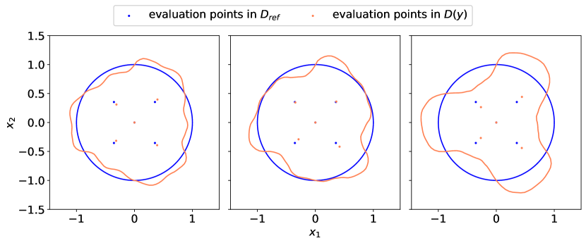
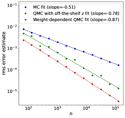
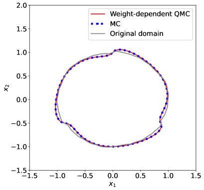
Figure 1: Fixed and transported evaluation points for three realizations, $k=5$.

Figure 2: Results corresponding to the Bayesian inverse problem ($\eta=10\%\|{\boldsymbol{\delta}}\|_{\infty}$, $k=5$). Left: Computed rms errors for the ratio estimator with increasing $n$ for the three methods. Right: The reconstructed domains for MC and QMC with $n=128021$ vis-à-vis the ground truth.

The data ${\boldsymbol{\delta}}$ given by (3) is generated after sampling from a truncated ${\boldsymbol{V}}$ with a stochastic dimension $s_{*}=200$ and discretizing the problem with a mesh size $h_{*}=2^{-6}$. We then obtain $(\delta_{0},\dots,\delta_{k-1})=(u_{s_{*},h_{*}}({\boldsymbol{V}}_{s_{*}}({\boldsymbol{x}}_{0},{\boldsymbol{y}})),\dots,u_{s_{*},h_{*}}({\boldsymbol{V}}_{s_{*}}({\boldsymbol{x}}_{k-1},{\boldsymbol{y}})))$. Finally, we set the noise level $\eta$ to $10\%$ of the maximum absolute value in ${\boldsymbol{\delta}}$.

To reconstruct the uncertain domain, we set a stochastic dimension $s=100$ and discretize the PDE solution with a mesh size $h=2^{-5}$. To test the convergence of the rms error as predicted in Theorem 3.6, we estimate the rms error using $R=8$ random shifts for prime values of $n$ ranging from $67$ to $128021$.

The results on the left-hand side of Figure 2 show the rms error for the approximation $\mathbb{E}_{s,h,n}[{\boldsymbol{V}}_{s}]$ with $k=5$ observation points. We observe a roughly linear convergence rate for the QMC approximation with the weights derived in Theorem 3.6, and hence an almost doubled rate with respect to the MC approach. The QMC approximation with an off-the-shelf generating vector ${\boldsymbol{z}}$ also performs consistently better than MC, but it exhibits a higher variance.

On the right-hand side of Figure 2, we present reconstructions for the weight-tailored QMC and the MC approximations. Due to the scaling of the parameters, both methods converge to the shown reconstructions already for small values of $n$. Nevertheless, the results indicate the consistency of the QMC approximation.

5 Conclusions

In this work, we have studied the application of randomly shifted rank-1 lattice rules to Bayesian shape inversion subject to Gevrey regular deformations of a reference domain with the Poisson equation as the forward model. Modeling the uncertain geometry using Gevrey regular perturbation fields covers a wider range of potential parameterizations than those covered by the affine or holomorphic frameworks, while also retaining a nearly optimal QMC convergence rate in the inverse setting as showcased by Theorem 3.6 and our numerical experiments. In addition, we showed that this setting leads to the optimal dimension truncation error rate as well as the standard FEM error rate.

The regularity analysis in this paper was presented for the pullback PDE solution. However, in many practical applications, it would be more natural to consider the pushforward PDE solution on the actual realization of the random or uncertain geometry instead. Our choice of the observation operator allows us to perform the experiments on the deformed domains while retaining the parametric regularity of the pullback PDE solution. Extending the regularity analysis for more general observation operators as well as more involved forward models is left for future work.

References

• (1) Bazahica, L., Kaarnioja, V., Roininen, L.: Uncertainty quantification for electrical impedance tomography using quasi-Monte Carlo methods. Preprint, arXiv:2411.11538 [math.NA] (2024)
• (2) Castrillón-Candás, J. E., Nobile, F., Tempone, R. F.: Analytic regularity and collocation approximation for elliptic PDEs with random domain deformations. Comput. Math. Appl. 71(6), 1173–1197 (2016)
• (3) Chernov, A., Lê, T.: Analytic and Gevrey class regularity for parametric elliptic eigenvalue problems and applications. SIAM J. Numer. Anal. 4(62), 1874–1900 (2024)
• (4) Chernov, A., Lê, T.: Analytic and Gevrey class regularity for parametric semilinear reaction-diffusion problems and applications in uncertainty quantification. Comput. Math. Appl. 164, 116–130 (2024)
• (5) Church, L., Djurdjevac, A., Elliott, C. M.: A domain mapping approach for elliptic equations posed on random bulk and surface domains. Numer. Math. 146, 1–49 (2020)
• (6) Cools, R., Kuo, F. Y., Nuyens, D.: Constructing embedded lattice rules for multivariate integration. SIAM J. Sci. Comput. 28, 2162–2188 (2006)
• (7) Dick, J., Kuo, F. Y., Sloan, I. H.: High-dimensional integration: the quasi-Monte Carlo way. Acta Numer. 22, 133–288 (2013)
• (8) Djurdjevac, A., Kaarnioja, V., Schillings, C., Zepernick, A.: Uncertainty quantification for stationary and time-dependent PDEs subject to Gevrey regular random domain deformations. Preprint, arXiv:2502.12345 [math.NA] (2025)
• (9) Dölz, J., Harbrecht, H., Jerez-Hanckes, C., Multerer, M.: Isogeometric multilevel quadrature for forward and inverse acoustic scattering. Comput. Methods Appl. Mech. Eng. 388, 114242 (2022)
• (10) Gantner, R. N., Peters, M. D.: Higher-order quasi-Monte Carlo for Bayesian shape inversion. SIAM/ASA J. Uncertain. Quantif. 6(2), 707–736 (2018)
• (11) Gilbarg, D., Trudinger, N. S.: Elliptic Partial Differential Equations of Second Order. Springer Berlin, Heidelberg (2001)
• (12) Grisvard, P.: Elliptic Problems in Nonsmooth Domains. Society for Industrial and Applied Mathematics (2011)
• (13) Guth, P. A., Kaarnioja, V.: Generalized dimension truncation error analysis for high-dimensional numerical integration: lognormal setting and beyond. SIAM J. Numer. Anal. 62(2), 872–892 (2024)
• (14) Guth, P. A., Kaarnioja, V.: Quasi-Monte Carlo for partial differential equations with generalized Gaussian input uncertainty. Preprint, arXiv:2411.03793 [math.NA] (2024)
• (15) Harbrecht, H., Peters, M., Siebenmorgen, M.: Analysis of the domain mapping method for elliptic diffusion problems on random domains. Numer. Math. 134, 823–856 (2016)
• (16) Harbrecht, H., Schmidlin, M., Schwab, Ch.: The Gevrey class implicit mapping theorem with application to UQ of semilinear elliptic PDEs. Math. Models Methods Appl. Sci. 34(5), 881–917 (2024)
• (17) Hyvönen, N., Kaarnioja, V., Mustonen, L., Staboulis, S.: Polynomial collocation for handling an inaccurately known measurement configuration in electrical impedance tomography. SIAM J. Appl. Math. 77, 202–223 (2017)
• (18) Kaarnioja, V., Schillings, C.: Quasi-Monte Carlo for Bayesian design of experiment problems governed by parametric PDEs. Preprint, arXiv:2405.03529 [math.NA] (2024)
• (19) Kaipio, J., Somersalo, E.: Statistical and Computational Inverse Problems. Springer, New York (2004)
• (20) Kuijpers, S., Scarabosio, L.: Wavenumber-explicit well-posedness of Bayesian shape inversion in acoustic scattering. Preprint, arXiv:2410.23100 [math.AP] (2024)
• (21) Kuo. F. Y.: Lattice rule generating vectors.
https://web.maths.unsw.edu.au/\textasciitildefkuo/lattice/
• (22) Kuo, F. Y., Nuyens, D.: Application of quasi-Monte Carlo methods to elliptic PDEs with random diffusion coefficients: a survey of analysis and implementation. Found. Comput. Math. 16(6), 1631–1696 (2016)
• (23) Kuo, F. Y., Schwab, Ch., Sloan, I. H.: Quasi-Monte Carlo finite element methods for a class of elliptic partial differential equations with random coefficients. SIAM J. Numer. Anal. 50(6), 3351–3374 (2012)
• (24) Nuyens, D., Cools, R.: Fast algorithms for component-by-component construction of rank-1 lattice rules in shift-invariant reproducing kernel Hilbert spaces. Math. Comp. 75, 903–920 (2006)
• (25) Quarteroni, A.: Numerical Models for Differential Problems. Springer Milano (2014)
• (26) Scheichl, R., Stuart, A. M., Teckentrup, A. L.: Quasi-Monte Carlo and multilevel Monte Carlo methods for computing posterior expectations in elliptic inverse problems. SIAM/ASA J. Uncertain. Quantif. 5(1), 493–518 (2017)
• (27) Somersalo, E., Cheney, M., Isaacson, D.: Existence and uniqueness for electrode models for electric current computed tomography. SIAM J. Appl. Math. 52(4), 1023–1040 (1992)
• (28) Stuart, A. M.: Inverse problems: a Bayesian perspective. Acta Numer. 19, 451–559 (2010)
• (29) Xiu, D., Tartakovsky, D. M.: Numerical methods for differential equations in random domains. SIAM J. Sci. Comput. 28(3), 1167–1185 (2006)