A hybrid minimizing movement and neural network approach to Willmore flow

Abstract

We present a hybrid method combining a minimizing movement scheme with neural operators for the simulation of phase field-based Willmore flow. The minimizing movement component is based on a standard optimization problem on a regular grid whereas the functional to be minimized involves a neural approximation of mean curvature flow proposed by Bretin et al. [8]. Numerical experiments confirm stability for large time step sizes, consistency and significantly reduced computational cost compared to a traditional finite element method. Moreover, applications demonstrate its effectiveness in surface fairing and reconstructing of damaged shapes. Thus, the approach offers a robust and efficient tool for geometry processing.

1 Introduction

Willmore flow is the $L^{2}$-gradient flow of the Willmore energy, which is defined as the surface integral over the squared mean curvature. For closed surfaces of genus zero, the Willmore energy allows to quantify how much a surface deviates from being a perfect sphere, with a round sphere having minimal Willmore energy. Physically, the Willmore energy reflects an approximation of the stored energy in a thin elastic shell with a planar physical reference configuration [12]. It is also used to model the behavior of cell membranes, which have tendency to minimize their bending. To this end, an extension of the Willmore energy, the Helfrich model, is used to describe elastic cell membranes in biology [11]. Furthermore, in computer graphics and geometry processing, Willmore flow is used for surface smoothing [14], and surface restoration [13, 34]. This motivates the study of Willmore flow, and in particular the development of numerical schemes.

However, as we will discuss below, Willmore flow is described by a fourth-order PDE, which makes it challenging to devise schemes that stably allow for large time steps and are computationally efficient. We will show that our proposed hybrid scheme is stable for large time steps and indeed leads to an efficient scheme for Willmore flow in case of a phase field formulation, which is in particular practical for applications with implicitly described geometries. To compute Willmore flow, we will consider a minimizing movement time discretization. Therein, we combine a discretization of the minimizing movement scheme on a regular grid with a neural network approximation of the mean curvature arising in the Willmore energy.

This paper deals with phase field models approximating hypersurfaces $\Gamma$ in the computational domain $\Omega=(0,1)^{d}$ and their evolution by Willmore flow. To motivate the hybrid method, we first recall the parametric formulation of Willmore flow. We denote by $x\colon\Gamma\to\Gamma$ the identity restricted to the surface $\Gamma$. Then the Willmore energy of $\Gamma$ is given by

$$w[x]\coloneqq\frac{1}{2}\int_{\Gamma}{\mathbf{h}}^{2}(x)\,\mathrm{d}\mathcal{H}^{d-1},$$ (1.1)

where ${\mathbf{h}}$ is the mean curvature. The Willmore flow for parametrizations is then the $L^{2}$-gradient flow of this energy, i.e. the evolution $x\colon[0,T]\times\Gamma\to\Omega$ that fulfills

$$(\partial_{t}x,\vartheta)_{L^{2}(\Gamma)}=-\partial_{x}w[x](\vartheta)$$ (1.2)

for all test functions $\vartheta\in C^{\infty}(\Gamma,\mathbb{R}^{d})$, where $(\cdot,\cdot)_{L^{2}(\Gamma)}$ denotes the $L^{2}$-scalar product on the hypersurface $\Gamma$ and $\partial_{x}w[x](\vartheta)$ the variation of the Willmore energy in direction $\vartheta$.

Willmore surfaces, i.e. minimizers of the Willmore energy, and Willmore flow have been the subject of intense theoretical study. Simonett proved in [46] the existence of a unique and locally smooth solution of Willmore flow for sufficiently smooth initial surfaces as well as exponential convergence to a sphere for initial surfaces close to a sphere. Similarly, Dall’Acqua et al. [15] proved that if the initial datum is a torus of revolution with Willmore energy less than $8\pi$ then the Willmore flow converges to the Clifford Torus. Kuwert and Schätzle treated long time existence and regularity of solutions in co-dimension one in [31, 32, 33] and Rivière [42] extended these results to arbitrary co-dimension. In 2014, Marques and Neves [35] were able to prove the famous Willmore conjecture, i.e. that for every smooth immersed torus in $\mathbb{R}^{3}$ the Willmore energy is lower bounded by $2\pi^{2}$.

Similarly, also the numerical treatment of Willmore flow for surfaces has garnered significant attention. Rusu [43] introduced a semi-implicit finite element scheme for the computation of the parametric Willmore flow of surfaces, which was applied by Clarenz et al. [13] to surface restoration problems. Droske and Rumpf [19] introduced a level set formulation for Willmore flow and corresponding numerical scheme. Deckelnick and Dziuk provided in [17] a-priori error estimates for a spatially discretized but time-continuous finite element scheme on two-dimensional graphs. Alternative finite element schemes for parametric Willmore flow were introduced by Barrett et al. [5] and Dziuk [23]. In contrast, Bobenko and Schröder [7] introduced a discrete Willmore energy and flow based on discrete differential geometry. Concerning phase field models, Du et al. introduced and analyzed a discrete semi-implicit scheme for Willmore flow in [20, 21]. In [9], Bretin et al. investigated flows for various diffuse approximations of the Willmore energy and its relaxations and introduced corresponding numerical schemes. If the goal is to minimize Willmore energy, one can also consider gradient flows with respect to other metrics. For example, Schumacher [45] analyzed $H^{2}$-gradient flows for the Willmore energy with numerical experiments on triangle meshes. Soliman et al. [47] extended this idea on triangle meshes to incorporate further constraints – most notably on the conformal class of the surface. However, in this paper, the goal is not to minimize the Willmore energy but to efficiently simulate Willmore flow, i.e. the $L^{2}$-gradient flow of the Willmore energy.

To this end, we will consider a variational time-discretization of Willmore flow based on the minimizing movements paradigm [16, 2]. In case of parametric Willmore flow and time step size $\tau>0$, given a parametrization $x^{k}\colon\Gamma\to\Omega$ approximating the evolution at time $k\tau$ , the next time step $x^{k+1}$ is given as the minimizer of

$$e[x^{k},x]\coloneqq\lVert x-x^{k}\rVert_{L^{2}(\Gamma^{k})}^{2}+2\tau\,w[x].$$ (1.3)

To obtain a fully implicit, variational formulation of Willmore flow that is (experimentally) unconditionally stable and allows for large step sizes, Balzani and Rumpf [3] proposed to approximate the Willmore functional $w[x]$ in Equation 1.3 using an approximate mean curvature. To this end, one denotes by $y_{\tilde{\tau}}[x]\colon\Gamma\to\Omega$ the solution of one discrete time step of mean curvature flow with time step size $\tilde{\tau}$ starting from the initial parametrization $x$ corresponding to the surface $\Gamma$. By definition, the mean curvature ${\mathbf{h}}$ is the normal velocity of mean curvature flow. Hence, $\frac{1}{2}\int_{\Gamma}\frac{|y_{\tilde{\tau}}[x]-x|^{2}}{\tilde{\tau}^{2}}\,\mathrm{d}\mathcal{H}^{d-1}$ constitutes a difference quotient approximation of the Willmore energy $w[x]$ and a minimizing movement functional is given as

$$e[x^{k},x]\coloneqq\|x-x^{k}\|_{L^{2}(\Gamma^{k})}^{2}+\tau\int_{\Gamma}\frac{|y_{\tilde{\tau}}[x]-x|^{2}}{\tilde{\tau}^{2}}\,\mathrm{d}\mathcal{H}^{d-1}.$$ (1.4)

As discrete solution for mean curvature motion, one might consider the time step of a semi-discrete backward Euler scheme with time step $\tilde{\tau}$ as proposed by Dziuk [22]. Thus, minimizing the energy $e[x^{k},x]$ in $x$ amounts to solving a nested time discretization with time discrete mean curvature motion as the inner and the actual time discrete Willmore flow as the outer problem, It can also be understood as a PDE-constrained optimization problem, where one optimizes the energy Equation 1.4 subject to the constraint that $y_{\tilde{\tau}}[x]$ is the solution of the linear discrete semi-implicit backward Euler scheme for mean curvature motion.

In this work, we pick up the approach proposed by Franken et al. [26] and focus on the corresponding scheme for phase fields. Our core idea is to construct a hybrid scheme where the inner problem is solved using a neural network, whereas the outer problem remains a classical minimizing movement optimization scheme. For the inner problem, we will build on recent work by Bretin et al. [8] on neural operators for time discrete mean curvature flow in a phase field formulation. These neural operators are efficient to evaluate, straightforward to differentiate, and convergent under spatial refinement in numerical experiments. By using them in the variational time-discretization, we obtain a numerical scheme for the phase-field approximation of Willmore flow that is stable for large time steps and still computationally efficient.

The remainder of the paper is organized as follows. In section 2, we recapitulate the adaption of the variational time-discretization to phase fields from [26] and introduce a neural operator approximation of mean curvature flow for phase fields inspired by [8]. We combine both to obtain the spatially discrete hybrid scheme for Willmore flow in section 3. In section 4, we first experimentally validate the convergence properties of the neural network based discrete mean curvature flow to then underpin a corresponding validation of our hybrid Willmore flow scheme. Furthermore, we use our hybrid scheme to compute the evolution for different interesting initial curves in 2D and surfaces in 3D. Afterwards, in section 5, we apply the scheme for curve and surface restoration. Finally, in section 6, we briefly draw conclusions.

2 Synthesis of the time discrete Willmore flow

Our scheme has two essential ingredients: a phase field based minimizing movement scheme for Willmore flow as introduced by Franken et al. [26], and a convolution based approximation of mean curvature. Below, we will first discuss the relevant parts of the former, then detail the latter and describe how both are combined for the purpose of an robust and efficient approximation of Willmore flow.

Phase field based minimizing movement scheme for Willmore flow.

Following Franken et al. [26] we assume that hypersurfaces under consideration are represented by Modica–Mortola-type phase field functions [38] with periodic boundary conditions. In what follows, we assume that all functions and interfaces are sufficiently smooth. We consider the interfacial energy

$$\mathcal{P}^{\varepsilon}[v]\coloneqq\frac{1}{2}\int_{\Omega}\varepsilon\lvert\nabla v\rvert^{2}+\frac{1}{\varepsilon}\Psi(v)\,\mathrm{d}x$$ (2.1)

with the double well potential $\Psi(v)=\frac{9}{16}(1-v^{2})^{2}$. Modica and Mortola [38] showed that the $\Gamma$-limit of $\mathcal{P}^{\varepsilon}[\cdot]$ in the $L^{1}$ topology is half the total variation of a function $u\in BV(\Omega;\{-1,1\})$ in $\Omega$, i.e. the perimeter of the set $\{u=1\}$.

phase field functions minimizing (2.1) follow an optimal profile in normal direction across the interface, which is $\tilde{v}_{\varepsilon}\colon\mathbb{R}\to\mathbb{R};\,s\mapsto\tanh(-\frac{3s}{4\varepsilon})$. Thus, $\tanh\left(-\frac{3}{4\varepsilon}\mathrm{sdist}(y,\omega)\right)$ is the optimal phase field profile of an interface $\Gamma=\partial\omega\cap\Omega$ for fixed $\varepsilon$, where the signed distance function of $\Gamma$ is defined as $\mathrm{sdist}(x,\omega)=\mathrm{dist}(x,\omega)-\mathrm{dist}(x,\omega^{c})$ with $\omega^{c}$ being the complement of $\omega$. Now, let $u^{k}_{\varepsilon}$ denote the phase field representations of the hypersurface $\Gamma^{k}$ with parametrization $x^{k}$, which is the boundary of a subset $\omega^{k}\subset\Omega$, i.e. $\Gamma^{k}=\partial\omega^{k}\cap\Omega$. Similarly, let $u_{\varepsilon}$ is the representation of $\Gamma=\partial\omega\cap\Omega$ with parametrization $x$, and $v_{\tilde{\tau}}[u_{\varepsilon}]$ a phasefield representation of the image of $\Gamma$ under timestep of mean curvature flow with step size $\tilde{\tau}$ and initial data $u_{\varepsilon}$.

To translate (1.4) to the phase field context, one observes for a shift $\delta$ of the optimal profile $\tilde{v}_{\varepsilon}$ in one dimension

$$\varepsilon\int_{\mathbb{R}} \left(\tilde{v}_{\varepsilon}(s)-\tilde{v}_{\varepsilon}(s-\delta)\right)^{2}\,\mathrm{d}s=\delta^{2}(1+\Theta(\delta,\varepsilon))\,,$$

where $\Theta(\delta,\varepsilon)=C\left(\frac{\delta}{\varepsilon}+\frac{\delta^{2}}{\varepsilon^{2}}\right)$. A detailed calculation is given in [26]. Chosing $\delta=\varepsilon^{\beta}$ with $\beta>1$ implies $\Theta(\delta,\varepsilon)\leq C\delta^{(1-\frac{1}{\beta})}$ and thus

$$\varepsilon\int_{\Omega}\left(u_{\varepsilon}(x+\delta(x)n(x))-u_{\varepsilon}(x)\right)^{2}\,\mathrm{d}x =\int_{\Gamma}\delta^{2}(x)\mathcal{H}^{d-1}\left(1+O(\Theta(\lVert\delta\rVert_{\infty},\varepsilon))\right)\,,$$

where now $\delta$ is some function on $\Gamma$, $n$ is the normal field of $\Gamma$ and $\delta$ is assumed to be extended constantly in normal direction to $\Gamma$. Next, assuming that all involved phase field functions $u^{k}$, $u$, and $v_{\tilde{\tau}}[u]$ follow the optimal profile, one observes that

$$\varepsilon\lVert v_{\tilde{\tau}}[u]-u\rVert_{L^{2}(\Omega)}^{2} =\lVert y_{\tilde{\tau}}[x]-x\rVert_{L^{2}(\Gamma)}^{2}\left(1+O(\Theta(\lVert y_{\tilde{\tau}}[x]-x\rVert_{L^{\infty}(\Gamma)},\varepsilon))\right),$$

$$\varepsilon\lVert u-u^{k}\rVert_{L^{2}(\Omega)}^{2} =\lVert x-x^{k}\rVert_{L^{2}(\Gamma^{k})}^{2}\left(1+O(\Theta(\lVert x-x^{k}\rVert_{L^{\infty}(\Gamma^{k})},\varepsilon))\right).$$

The above estimates were presented in [26] using the double well function $\Psi(v)=(1-v^{2})^{2}$ and thus consistently with an additional factor $\tfrac{4}{3}$ (and optimal profile $\tilde{v}_{\varepsilon}(s)=\tanh(-s\varepsilon^{-1})$).

Finally, with these approximations at hand, one can define the energy

$$e^{\varepsilon}[u^{k},u]=\varepsilon\lVert u-u^{k}\rVert_{L^{2}(\Omega)}^{2}+\frac{\tau\varepsilon}{\tilde{\tau}^{2}}\lVert v_{\tilde{\tau}}[u]-u\rVert_{L^{2}(\Omega)}^{2}$$ (2.2)

for two functions $u^{k}$ and $u$ considered as phase field descriptions of $\Gamma^{k}$ and $\Gamma$. By our above estimates this energy is equivalent to the energy $e[\cdot]$ associated with the variational time-discretization in Equation 1.4.

Altogether for sufficiently small phase field parameter $\varepsilon$ and sufficiently small time step sizes $\tau$, $\tilde{\tau}$ this leads to the following nested variational time discretization of Willmore flow:

Definition 2.1 (Variational time discretization of Willmore flow [26]).

For $e^{\varepsilon}[\cdot,\cdot]$ defined in Equation 2.2 based on some mapping $v_{\tilde{\tau}}:L^{2}(\Omega)\to L^{2}(\Omega)$ with $\tau,\;\tilde{\tau}>0$ and some $u^{0}\in L^{2}(\Omega)$ we iteratively compute

$$u^{k+1}=\operatorname*{arg\,min}_{u\in L^{2}(\Omega)}e^{\varepsilon}[u^{k},u]$$ (2.3)

as the time discrete phase field solution at time $(k+1)\tau$ for $k\in\mathbb{N}_{0}$.

Convolution based approximation of mean curvature.

We are still left to define $v_{\tilde{\tau}}[u]$ variationally. Again following Franken et al. [26] we take into account a further minimizing movement scheme, now for mean curvature motion and define

$$v_{\tilde{\tau}}[u]\coloneqq\operatorname*{arg\,min}_{v\in H^{1}(\Omega)}\left(\varepsilon\|u-v\|^{2}_{L^{2}(\Omega)}+2\tilde{\tau}\mathcal{P}^{\varepsilon}[v]\right)$$ (2.4)

as the inner variational problem to be solved for every $u$ in the outer problem Equation 2.3. Instead of solving the Euler-Lagrange equation associated with Equation 2.4 for every function $u$ arising in the outer problem we pick up the approach by Bretin et al. [8] and combine a nonlinear activation function and a convolution operator to define a still spatially continuous approximation of ${v}_{\tilde{\tau}}[\cdot]$. In fact, the general, spatially continuous structure of the scheme in [8] is given by a spatially continuous neural operator

$$v^{f,\kappa}_{\tilde{\tau}}[u]=f_{\tilde{\tau}}\circ(\kappa_{\tilde{\tau}}*u),$$ (2.5)

where one first applies a convolution kernel $\kappa_{\tilde{\tau}}\in L^{2}(\mathbb{R}^{d})$, followed by the concatenation with a nonlinear activation function $f_{\tilde{\tau}}\in C^{0}(\mathbb{R})$. When applying the kernel $\kappa_{\tilde{\tau}}$ to $u$ we assume that $u$ is periodically extended to all of $\mathbb{R}^{d}$. The convolution $\kappa_{\tilde{\tau}}\ast u$ with $\kappa_{\tilde{\tau}}\in L^{2}(\mathbb{R}^{d})$ is in $C^{0}(\mathbb{R}^{d})$. Thus, $v^{f,\kappa}_{\tilde{\tau}}[u]\in C^{0}(\mathbb{R}^{d})$ as well and can in particular be evaluated point-wise.

The resulting time discrete but spatially still continuous scheme combines a standard optimization problem over functions in $L^{2}(\Omega)$ with a neural operator acting on functions in $L^{2}(\Omega)$.

Remark 2.2 (Relation to the MBO scheme and semi-implicit time stepping for Allen-Chan flow).

To motivate the neural networks architecture used by Bretin et al. we first observe that the rescaled $L^{2}$-gradient flow of $\mathcal{P}^{\varepsilon}$ with time discretization Equation 2.4 is given by the Allen–Cahn equation $\partial_{t}u-\Delta u+\tfrac{1}{2\varepsilon^{2}}\Psi^{\prime}(u)=0.$ Evaluating the nonlinearity $\Psi^{\prime}$ implicitly at $u^{k+1}$ and the Laplace operator explicitly at $u^{k}$ we obtain the time-discrete equation

$$\tfrac{u^{k+1}-u^{k}}{\tilde{\tau}}-\Delta u^{k}+\tfrac{1}{2\varepsilon^{2}}\Psi^{\prime}(u^{k+1})=0$$ (2.6)

to iteratively compute the sequence $(u^{k})_{k\in\mathbb{N}}$ of phase fields given an initial phase field $u^{0}$. The function $\phi_{\varepsilon,\tilde{\tau}}(u)=u+\frac{\tilde{\tau}}{2\varepsilon^{2}}\Psi^{\prime}(u)$ is monotone for $\frac{\tilde{\tau}}{\varepsilon^{2}}<\frac{8}{9}$ and thus invertible. Hence, Equation 2.6 can be rewritten as $u^{k+1}=\phi_{\varepsilon,\tilde{\tau}}^{-1}((\mathrm{Id}+\tilde{\tau}\Delta)u^{k})$ and finally using the approximation $(\mathrm{Id}+\tilde{\tau}\Delta)u^{k}=e^{-\tilde{\tau}\Delta}u^{k}+O(\tilde{\tau}^{2})$ we obtain $u^{k+1}=\phi^{-1}(e^{-\tilde{\tau}\Delta}u^{k}).$ This indeed reflects the structure Equation 2.5 proposed by Bretin et al. [8] and resembles the Merriman–Bence–Osher (MBO) scheme [36, 37] for characteristic functions where one first solves the linear heat equation with time step $\tilde{\tau}$ for a characteristic function as the initial data and then applies a thresholding function to obtain the time step updated characteristic function. In this sense, the application of the function $\phi_{\varepsilon,\tilde{\tau}}^{-1}$ acts as a soft thresholding. For the convergence to mean curvature motion, we refer to [24] and [4]. Recently, Budd and van Gennip [10] studied a semi-implicit time-discretization for the double obstacle Allen–Cahn equation on graphs and proved that the MBO scheme coincides with a particular choice of a semi-implicit scheme for Allen–Cahn flow. The scheme takes the form $u^{k+1}=\rho\circ\left(e^{-\tilde{\tau}\Delta}u^{k}\right)$, with $\Delta$ being the (positive definite) graph Laplacian, $\rho$ a monotone Lipschitz continuous (activation) function, and $e^{-\tilde{\tau}\Delta}$ the linear operator representing one timestep of the heat flow with time step size $\tilde{\tau}$. The authors explicitly refer to the analogy of a convolutional neural network in [10, footnote 6].

As proposed in [8], both the kernel $\kappa_{\tilde{\tau}}$ and the scalar function $f_{\tilde{\tau}}\in C^{0}(\mathbb{R})$ are to be learned from data. Bretin et al. suggested to consider (discrete) phase field profiles for the explicitly known evolution of hyperspheres in $\mathbb{R}^{d}$ as training data. In the spatially continuous case, we denote by $R(r_{0},\tilde{\tau})=\sqrt{r_{0}^{2}-2(d-1)\tilde{\tau}}$ the radius of the sphere evolution under mean curvature motion at time $\tilde{\tau}$ for initial radius $r_{0}$ and by $u_{r}\colon x\mapsto\tanh\left(\frac{3(r-|x|)}{4\varepsilon}\right)$ the phase field profile for a hypersphere with radius $r$ and determine $f_{\tilde{\tau}}$ and $k_{\tilde{\tau}}$ as solutions of the optimization problem

$$\min_{f,\kappa}\int_{r_{\mathrm{min}}}^{r_{\mathrm{max}}}\rVert v^{f,\kappa}_{\tilde{\tau}}[u_{r}]-u_{R(r,\tilde{\tau})}\lVert^{2}_{L^{2}(\mathbb{R}^{d})}\,\mathrm{d}r$$ (2.7)

where one optimizes over suitable classes of nonlinear functions $f$ and convolution kernels $\kappa$ for a suitable choice of $r_{\mathrm{min}}$ and $r_{\mathrm{max}}$ .

Remark 2.3.

In their study Bretin et al. [8] focused on a discrete formulation on regular grids and directly developed a time and space discrete evolution operator for mean curvature motion. The underlying neural network consists of a single convolution layer and a scalar activation function realized with a multilayer perceptron. Bretin et al. demonstrated empirically that this also leads to a reasonable approximation of mean curvature flow for fairly general initial data and corresponding phase fields. Functions of the form Equation 2.5 are efficient to evaluate and differentiate when implemented on discrete grids using neural networks. We will retrieve this discrete formulation in the next section.

Furthermore, employing the scheme composed of Equation 2.2 and Equation 2.5, we can show the existence of time-discrete Willmore flow:

Proposition 2.4.

For $\Omega=(0,1)^{d}$, $u^{0}\in L^{2}(\Omega)$ periodically extended on $\mathbb{R}^{d}$, and $e^{\varepsilon}[u^{0},\cdot]$ as in (2.2) with $v_{\tilde{\tau}}$ of the form $v_{\tilde{\tau}}[u]=f(\kappa\ast u)$ for $f\in C(\mathbb{R})$ and $\kappa\in L^{2}(\mathbb{R}^{d})$ there exists a minimizer $u\in L^{2}(\Omega)$ of $e^{\varepsilon}[u^{0},\cdot]$ in the class of periodically extended $L^{2}(\Omega)$ functions.

Proof.

Let $(u_{j})_{j}\subset L^{2}(\Omega)$ be a minimizing sequence of $e^{\varepsilon}[u^{0},\cdot]$, with

$$C=e^{\varepsilon}[u^{0},u^{0}]\geq e^{\varepsilon}[u^{0},u_{j}]\geq\varepsilon\|u^{0}-u_{j}\|^{2}_{L^{2}(\Omega)}\geq\frac{\varepsilon}{2}\|u_{j}\|^{2}_{L^{2}(\Omega)}-\varepsilon\|u^{0}\|^{2}_{L^{2}(\Omega)}\,,$$

for a constant $C$ depending on $\|u^{0}\|_{L^{2}(\Omega)}$. Here, we used that $\|\kappa\ast u_{0}\|_{C^{0}(\bar{\Omega})}$ is bounded and applied Young’s inequality. Hence, $\|u_{j}\|_{L^{2}(\Omega)}\leq\hat{C}$ for some constant $\hat{C}$, and thus there exists $u\in L^{2}(\Omega)$, and a subsequence (not relabeled), with $u_{j}\rightharpoonup u$ weakly in $L^{2}(\Omega)$. Once more using that $\kappa\in L^{2}(\mathbb{R}^{d})$, we have

$$(\kappa\ast u_{j})(x)=\int_{\Omega}\kappa(x-y)u_{j}(y)\,\mathrm{d}y\rightarrow\int_{\Omega}\kappa(x-y)u(y)\,\mathrm{d}y=(\kappa\ast u)(x)$$

for $j\rightarrow\infty$. Furthermore, we observe

$$\sup_{x\in\Omega}\left|(\kappa\ast u_{j})(x)\right|\leq\|\kappa\|_{L^{2}(\mathbb{R}^{d})}\|u_{j}\|_{L^{2}(\Omega)}\leq\hat{C}\|\kappa\|_{L^{2}(\mathbb{R}^{d})}.$$

Since $f$ is uniformly continuous on $[-\hat{C}\|\kappa\|_{L^{2}(\mathbb{R}^{d})},\hat{C}\|\kappa\|_{L^{2}(\mathbb{R}^{d})}]$, we obtain $f(\kappa\ast u_{j})\rightarrow f(\kappa\ast u)$ pointwise and in $L^{2}(\Omega)$. Finally, lower semicontinuity of the $L^{2}$ norm implies

$$\inf_{\tilde{u}\in L^{2}(\Omega)}e^{\varepsilon}[u^{0},\tilde{u}]=\liminf_{j\rightarrow\infty}e^{\varepsilon}[u^{0},u_{j}]\geq e^{\varepsilon}[u^{0},u].$$

Thus $u\in L^{2}(\Omega)$ and minimizes $e^{\varepsilon}[u^{0},\cdot]$ in the class of periodically extended $L^{2}(\Omega)$ functions. ∎

3 Spatial discretization

Minimizing movement scheme for Willmore flow.

To discretize the time-discrete Willmore flow in $\mathbb{R}^{d}$ based on the minimizing movement scheme Equation 2.2, we consider a regular grid on $[0,1]^{d}$ with gridsize $h=\tfrac{1}{n}$ for $n\in\mathbb{N}$ and nodes $x_{\alpha}=(\tfrac{\alpha_{1}}{n},\cdot,\tfrac{\alpha_{d}}{n})$ for a multi-index $\alpha$ in the multi index set $\mathcal{I}_{n}\coloneqq(\{0,\ldots,n\})^{d}$. On this grid we consider functions represented by nodal vectors $U\in\mathbb{R}^{|\mathcal{I}_{n}|}$ with function values $U_{\alpha}$ at nodes $x_{\alpha}$. A discrete $L^{2}$ norm is defined as

$$\lVert U\rVert_{L^{2}}\coloneqq\sqrt{(n+1)^{-d}\sum_{\alpha\in\mathcal{I}_{n}}(U_{\alpha})^{2}},$$

i.e. the square root of the average of the squared entries of $U$. Thus, the discrete counterpart of the energy Equation 2.2 is given by

$$E^{\varepsilon}[U^{k},U]=\varepsilon\lVert U-U^{k}\rVert_{L^{2}}^{2}+\frac{\tau\varepsilon}{\tilde{\tau}^{2}}\lVert V_{\tilde{\tau}}[U]-U\rVert_{L^{2}}^{2},$$ (3.1)

where $V_{\tilde{\tau}}[U]$ denotes a spatially discrete counterpart of Equation 2.5.

Neural approximation of discrete mean curvature flow.

Here, we follow the approach by Bretin et al. [8] and consider discrete kernels and a nonlinear activation functions which are defined themselves as networks. For a discrete kernel $K\in\mathbb{R}^{\mathbb{Z}^{d}}$, one defines the nodal vector resulting from the discrete convolution with this kernel as

$$(K\ast U)_{\alpha}\coloneqq\sum_{\beta\in\mathbb{Z}^{d}}K_{\beta}U_{\alpha+\beta}.$$

Here, we assume periodicity of the discrete function to which we apply the discrete convolution, i.e. $U_{\alpha+\beta n}=U_{\alpha}$ for $\beta\in\mathbb{Z}^{d}$. Now, one considers discrete kernels with a fixed width $n_{K}$ and a $n_{K}^{d}$ stencil, i.e. $K_{\alpha}=0$ for $\max_{i=1,\ldots,d}|\alpha_{i}|>\tfrac{n_{K}-1}{2}$. To ensure consistency with the continuous mean curvature motion the necessary size $n_{K}$ of the kernel depends on the time step size $\tilde{\tau}$ and the grid size $h$. At the same time, smaller kernels are more efficient to train which creates a trade-off between accuracy and speed. This trade-off will be explored in our numerical experiments below. The point-wise function $f$ is discretized using a fully-connected neural network $F^{\theta}\colon\mathbb{R}\to\mathbb{R}$ with $L$ layers and layer sizes $N_{1},\ldots,N_{L}$. The $l$th layer is described in terms of a weight matrix $W^{l}\in\mathbb{R}^{N_{l}\times N_{l-1}}$ with $N_{0}=1$ and a bias vector $b^{l}\in\mathbb{R}^{N_{l}}$. These degrees are gathered in a parameter vector $\theta=(W^{1},\ldots,W^{L},b^{1},\ldots,b^{L})$. Then, one defines $F^{\theta}(s)=s^{L}$ with $s^{l}\coloneqq\rho\left(W^{l}s^{l-1}+b^{l}\right)$ and $s^{0}=s$ and the choice $\rho(s)=\exp(-s^{2})$ as the nonlinear activation function. In practice, we used six layers with sizes $32,\,16,\,8,\,4,\,2,\,1$. For given parameters $\theta$ and $K$, we obtain the discrete operator

$$V^{\theta,K}_{\tilde{\tau}}[U]\coloneqq F^{\theta}(K\ast U).$$ (3.2)

Now, one approximates the optimization problem Equation 2.7 via our discretization and a sampling of training data. To this end, one considers $m$ radii $r_{1},\ldots,r_{m}$ sampled uniformly from an interval $[r_{\mathrm{min}},r_{\mathrm{max}}]$ and minimizes the loss functional

$$\mathcal{L}[\theta,K]=\frac{1}{m}\sum_{i=1}^{m}\rVert V^{\theta,K}_{\tilde{\tau}}[U_{r_{i}}]-U_{R(r_{i},\tilde{\tau})}\lVert^{2}_{L^{2}},$$ (3.3)

over the total set of parameters $(\theta,\rho)$, where $U_{r}$ are nodal evaluations of the hypersphere phase fields $u_{r}$. We approximately solve problem Equation 3.3 using the Adam optimizer [29], with $m=100$, $r_{\mathrm{min}}=0.05$, $r_{\mathrm{max}}=0.4$, and usually employ mini-batching, i.e. approximating the sum in Equation 3.3 using only ten randomly drawn radii, to speed-up the minimization as was proposed by Bretin et al. [8]. The resulting neural phase field operator $V^{\theta,K}_{\tilde{\tau}}[\cdot]$ approximates the PDE solution $v_{\tilde{\tau}}$ defined in Equation 2.4 and is inexpensive to evaluate.

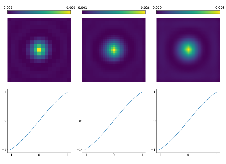
Figure 1: Learned networks for $\varepsilon=2^{-6}$ and $\tilde{\tau}=2^{-14}$ are displayed via a color coding of the learned kernels $K$ and the graphs of learned activation function $F^{\theta}$ on the interval $[-1,1]$ for increasing $n=128,\,256,\,512$, with stencil widths $n_{K}=17,\,33,\,65$, respectively.

We employ Newton’s method with Armijo line search to minimize $E^{\varepsilon}[U^{k},U]$ over $U$. Thus, to determine the descent direction $P$, we approximately solve the linear system $D^{2}E^{\varepsilon}[U^{k},\cdot]P=DE^{\varepsilon}[U^{k},\cdot]$ using the conjugated gradient method (see [40, Chapter 7]). This also prevents us from having to assemble the Hessian and we instead only compute the corresponding matrix-vector product. Furthermore, we manually implemented the derivatives of $E^{\varepsilon}[U^{k},\cdot]$ to improve performance. We developed our hybrid method in Python using the PyTorch library [41] and the nonlinear optimization algorithms used in the pytorch-minimize [25] package, which is based on the optimization module of SciPy [48].

4 Numerical experiments

As usual in nonlinear optimization, the chosen initialization when solving Equation 3.3 impacts the result. For example, Bretin et al. [8] successfully trained their network on a resolution of $n=256$ with stencil width $n_{K}=17$, $\varepsilon=2h$, and $\tilde{\tau}=\varepsilon^{2}$. They initialized the kernel as zero and the parameters $\theta$ randomly sampled from a normal distribution. However, when refining $h$ while keeping $\varepsilon$ fixed, and thus consistently increasing $n_{K}$, we observed a degradation of the approximation quality of $V^{\theta,K}_{\tilde{\tau}}[\cdot]$. We mitigated this by first training the network on a coarse resolution as proposed by Bretin et al. and then progressively passing to finer resolutions. In each step, we initialize the kernel using a bilinear interpolation of the coarser one. For the nonlinearity $F^{\theta}$, we kept the previous parameters as initialization. The resulting networks are displayed in Figure 1.

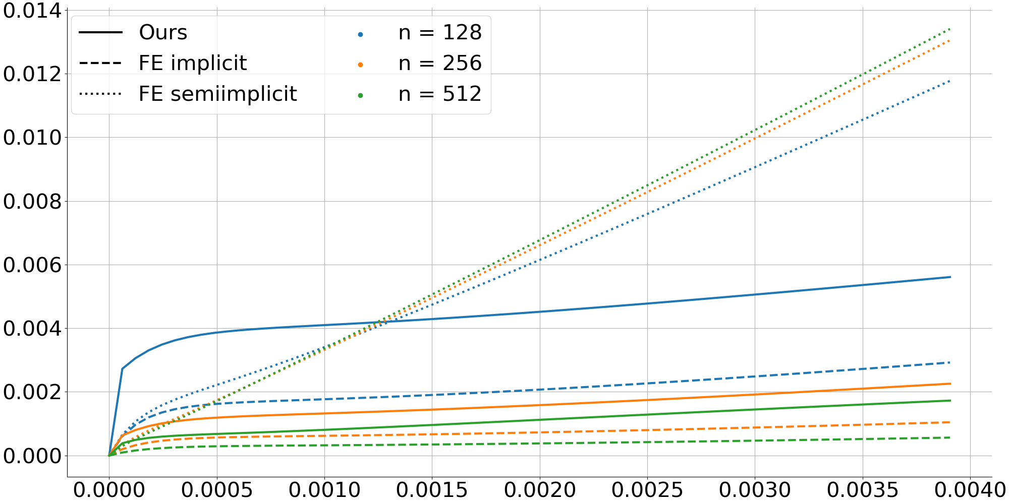
Figure 2: Convergence validation for mean curvature flow with fixed $\varepsilon=2^{-6}$ and $\tilde{\tau}=2^{-14}$ while increasing $n$, with $n_{K}=\tfrac{n}{8}+1$. We plot the average $L^{2}$-error to the analytic solution along time for 30 circles with radii $r_{i}=0.05\pi+\tfrac{0.15\pi i}{30}\,$, $i=0,\dots,29$. The line-styles correspond to the different methods and the colors to the varying resolution. For comparison: for the averaged $L^{2}$ distance between the solution at time $0.004$ and at the initial time zero, one obtains $\tfrac{1}{30}\sum_{i=1}^{30}\|U_{R(r_{i},0.004)}-U_{R(r_{i},0)}\|_{L^{2}}\approx 0.133$.

With this setup, we first investigate the convergence of the neural network-based MCF scheme Equation 3.2 and Equation 3.3 in two dimensions under spatial refinement, i.e. we keep the scale parameter $\varepsilon$ and the time step size $\tilde{\tau}$ fixed and increase the spatial resolution and the width of the kernel $n_{K}$. We compare the neural network scheme by Bretin et al. [8] with a fully implicit (cf. Equation 2.4) and semi-implicit finite element scheme. In the latter, one computes the solution $v$ at next timestep as the solution of $\frac{v-u}{\tilde{\tau}}=\Delta v-\tfrac{1}{2\varepsilon^{2}}\Psi^{\prime}(u)$ for given $u$ at the current timestep. Here, we consider a multi-linear finite element approach on the regular quad mesh. We perform the validation of convergence for the evolution of circles on the computational domain $\Omega=(-1,1)^{2}$. In Figure 2, we plot the average error when comparing to the exact solution over 30 radii ranging from $0.05\pi$ to $0.2\pi$. The error is displayed along 64 timesteps of size $\tilde{\tau}=2^{-14}$ for the different schemes and varying resolution.

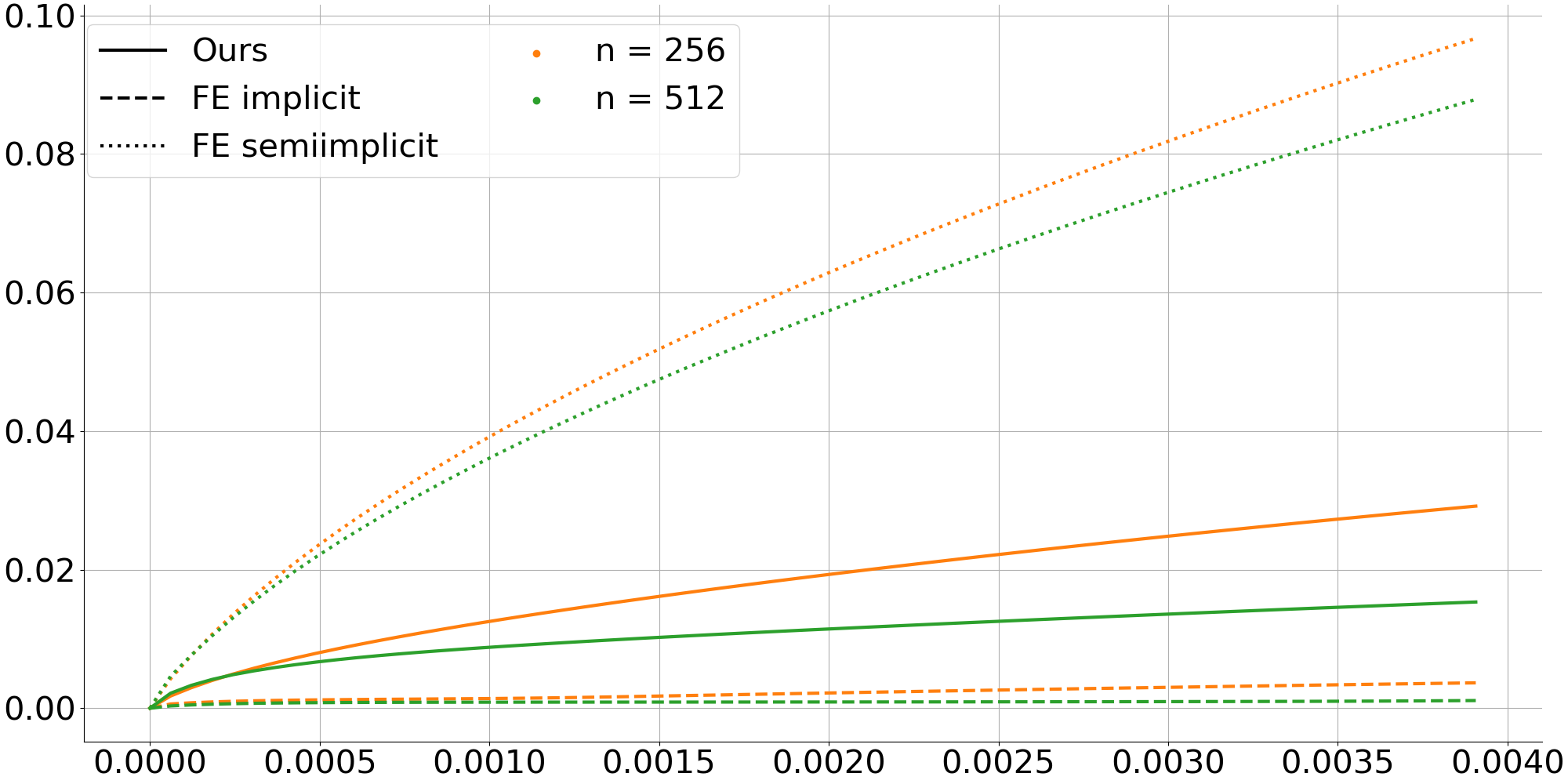
(a) Circles

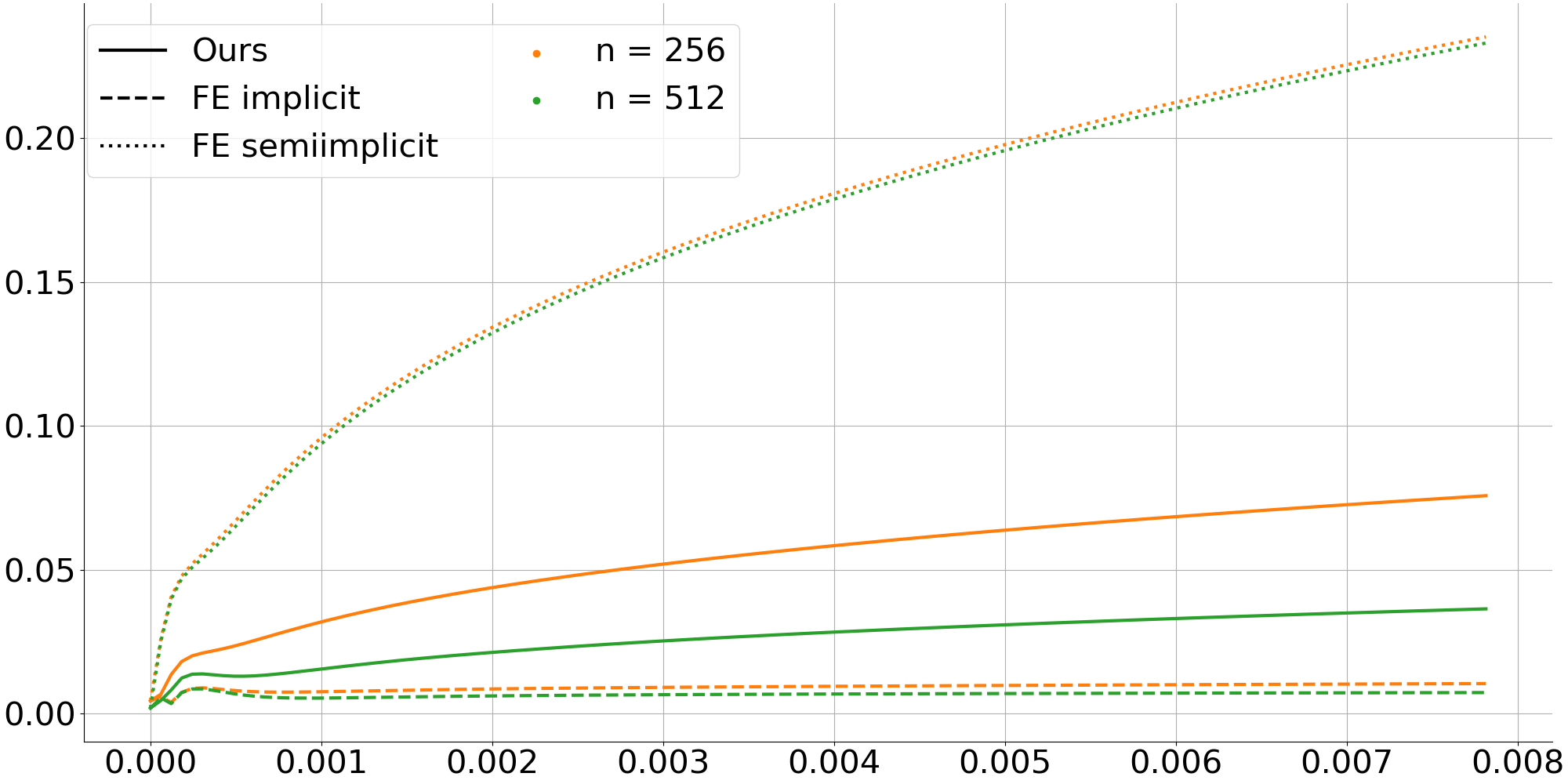
(b) Rectangle

Figure 3: Convergence tests for Willmore flow with fixed $\varepsilon=2^{-6}$ and $\tilde{\tau}=2^{-14}$ while increasing $n$, with $n_{K}=\tfrac{n}{8}+1$. As in Figure 2, the line-styles correspond to the different methods for approximating the mean curvature evolution and the colors to the varying resolution. In (a), we plot the average $L^{2}$-error to the analytic solution for 30 circles with radii $r_{i}=0.05\pi+\tfrac{0.15\pi i}{30}\,$, $i=0,\dots,29$ over time. For comparison: for the averaged $L^{2}$ distance between the solution at time $0.004$ and at the initial time zero, one obtains$\tfrac{1}{30}\sum_{i=1}^{30}\|U_{R_{W}(r_{i},0.004)}-U_{R_{W}(r_{i},0)}\|_{L^{2}}\approx 0.414$. In (b), we plot the $L^{2}$-error of the evolution of a rectangle sized $0.4\times 0.2$ compared to a fine implicit finite element solution ($n=2048$).

One observes that the neural network-based MCF scheme performs noticeably better than the semi-implicit finite element scheme. This confirms the observations made by Bretin et al. [8] for a single resolution. The fully implicit FE scheme outperforms the network-based scheme, which is not that surprising due to its semi-implicit nature. In summary, the network-based scheme positions itself between semi-implicit and fully implicit finite element scheme in terms of accuracy.

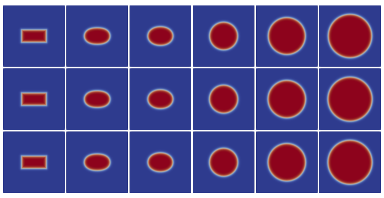
Figure 4: Willmore flow of a rectangle with side lengths $0.4\times 0.2$ using $\varepsilon=2^{-6}$. Results of our hybrid scheme on resolution $n=256$ (top row), fully implicit finite element solution of the nested scheme on resolution $n=256$ (middle row) and on resolution $n=2048$ (bottom row). From left to right: evolution times $t=0,\,2^{-14},\,2^{-13},\,2^{-10},\,2^{-8},\,2^{-7}$, respectively.

In two dimensions, the evolution of a circle with initial radius $r$ under Willmore flow is given at time $\tau$ by a circle with radius $R_{W}(r,\tau)=\sqrt[{}^{4}]{r^{4}+2\tau}$. In 3(a), the error of our hybrid scheme based on Equation 2.2, Equation 3.2 is displayed averaging over the same set of initial radii as in Figure 2. Again, the different line-styles (solid, dashed, dotted) correspond to the different methods for solving the inner MCF problem (hybrid, finite element implicit and semi-implicit). As shown in [26], for $\varepsilon=2h$ ($h=\tfrac{1}{n}$), the nested Willmore scheme suffers from numerical instabilities. Hence, we only consider the error evolution for $n=256,\,512$ and for fixed $\varepsilon=2^{-6}$.

To test our scheme not only on circles, on which the networks were trained, we applied the hybrid scheme to initial data given as the phase field approximation of a rectangle sized $0.4\times 0.2$. Since there is no known analytic solution for Willmore flow in this case, we compare the results to a solution of the nested finite element scheme by Franken et al. [26] on a much finer resolution ($n=2048$). The corresponding error evolution is displayed in 3(b). In both experiments, we observe that our hybrid approach performs noticeably better than the nested scheme using a semi-implicit finite element approach for the inner MCF problem, while the fully implicit nested finite element scheme from [26] remains the most accurate. This mirrors the observations for MCF.

From now on, we focus on our hybrid scheme. In Figure 4, we show the evolution of the rectangle under Willmore flow. We observe that already for the coarser resolution (e.g. $n=256$) the results are qualitatively indistinguishable from those computed with fine resolution ($n=2048$). Hence, for applications where one is primarily interested in the qualitative effects of Willmore flow, one can effectively achieve satisfying results on coarser resolutions. We will exploit this in the next section.

We end this section with a few details on the implementation and data processing pipeline. As for our hybrid scheme (see section 3), we have implemented the finite element-based approaches in Python using standard libraries. We implemented the nested scheme using Newton’s method as described in [26] with direct linear solver PARDISO [44]. All experiments using the finite element-based approaches were run on a workstation with two 32-core AMD EPYC 7601 processors with 1TB RAM. All experiments using our hybrid approach were run on a workstation with an NVIDIA A100 GPU with 40GB of memory and two 24-core AMD EPYC 7402 processors with 256GB RAM using double-precision floating-point arithmetic on the GPU. The phase fields for the armadillo and the rocker-arm were generated as follows: First, using the tool mesh_to_voxels from [30] signed distances were generated on a $n^{3}$ grid based on corresponding meshes. Then, the optimal phase field profile, as described in section 2, was applied to the signed distances. To generate the images in Figure 9 and in Figure 6, the zero-levelset of the phasefield was extracted using the Contour function from Paraview [1]. Finally, all results in 3D were rendered in Blender [6].

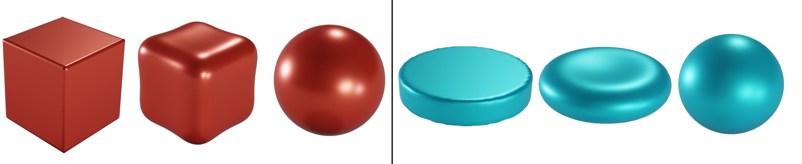
Figure 5: Evolution by Willmore flow for a cube surface and a thick disk surface with spatial resolution $n=64$, kernel size $n_{K}=17$, interface parameter $\varepsilon=2^{-5}$, inner stepsize $\tilde{\tau}=2^{-12}$, and Willmore flow stepsize $\tau=2^{-18}$. Results are shown at time $0,1$, and time $10$, which reproduce concave surface patches as common effects for Willmore.

5 Applications in image and geometry processing

Now that we have introduced and studied our proposed scheme, we will briefly discuss its use for two closely-related applications: surface fairing and surface restoration.

In the first of these applications, surface fairing, the goal is to create a visually smooth and seamless surface starting from an input surface that is usually noisy or otherwise corrupted. The problem has been studied in the computer graphics and vision communities and curvature flows have established themselves as a classical tool [18]. Willmore flow is particularly interesting as a basic model for this application [7, 27, 47] since it avoids singularities that could arise with mean curvature flow [14]. Hence, we consider the Willmore flow of surfaces in $\mathbb{R}^{3}$ for corresponding initial surfaces in Figure 5 and see that our scheme is able to reproduce common effects of Willmore flow. We furthermore apply it to the armadillo, often referenced in computer graphics, in Figure 6 and a rocker-arm model in Figure 7. Concerning computational cost, we show the results comparing our hybrid scheme to the original finite element-based nested Willmore approach by Franken et al. [26] in Table 1.

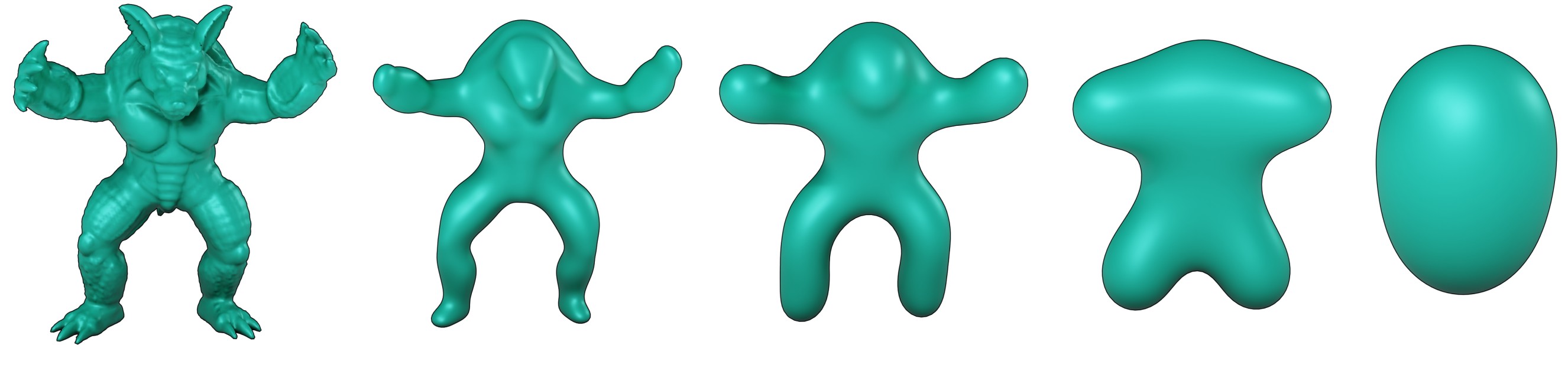
Figure 6: Evolution of the armadillo shape under Willmore flow. The spatial resolution is $n=128$, the kernel size is $n_{K}=17$, the interface parameter $\varepsilon=2^{-6}$, the inner stepsize $\tilde{\tau}=2^{-14}$, and the Willmore flow stepsize $\tau=2^{-20}$. Results are shown at time $0,1,4,40$, and $400$, respectively.

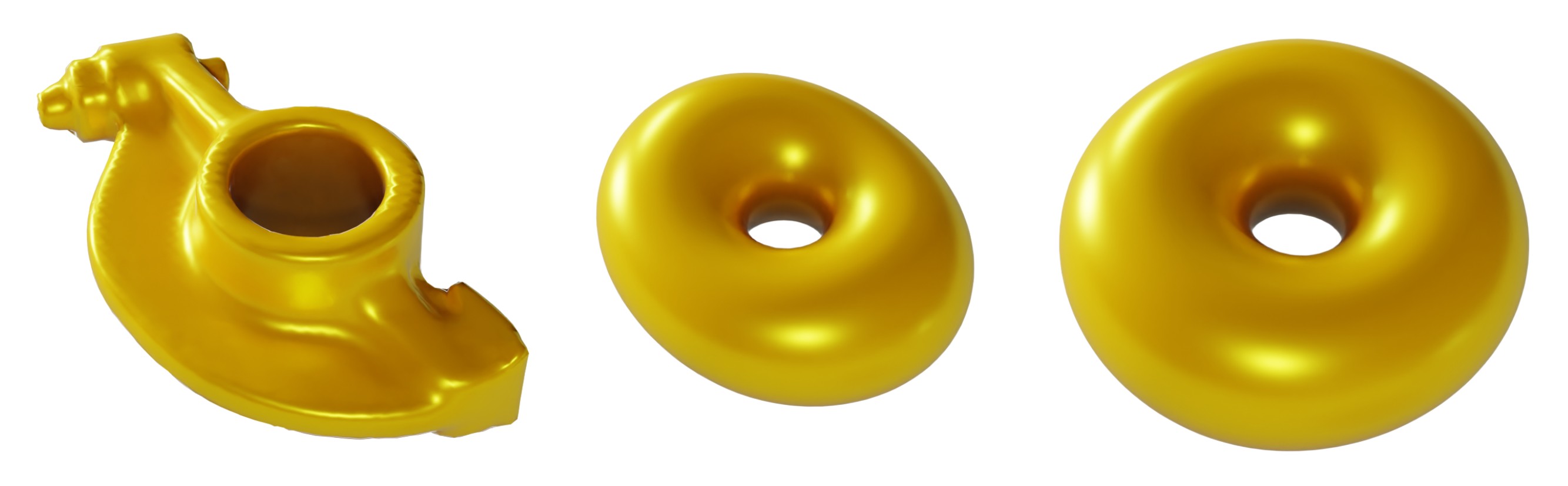
Figure 7: Evolution of a rocker arm shape under Willmore flow. The spatial resolution is $n=64$, the kernel size is $n_{K}=17$, the interface parameter $\varepsilon=2^{-5}$, the inner MCF stepsize $\tilde{\tau}=2^{-12}$, and the Willmore flow stepsize $\tau=2^{-12}$. We show the discrete timesteps $0,1$, and $20$ leading to an approximation of the Clifford torus.

Method	Armadillo (N=64)
nested FEM [26]	14589 sec
Ours	807 sec

Table 1: Performance comparison of our hybrid method to the nested finite element scheme by Franken et al. [26] on the example from Figure 6: The results after one step of Willmore flow starting from the shape on the far-left of Figure 6 (right), computing time (left).

The second application we consider, surface inpainting, is a fundamental topic in geometry and image processing, where one aims to restore corrupted or destroyed parts of an image or a surface. We investigate in this section the use of our hybrid approach to tackle this problem. In a first step, one replaces the corrupted or missing part by an ansatz geometry, whose primary purpose is to prescribe the desired topology. Following the edge restoration approach by Nitzberg et al. [39], one considers the energy (2.2) on the full domain $\Omega$, but only takes into account degrees of freedom in a part $D\subset\Omega$, where the image or surface is corrupted. Then, Willmore flow under this constraint leads to smooth reconstructions of the corrupted area while preserving $C^{1}$ boundary conditions on $\partial D\cap\Omega$. We illustrated two examples in two dimensions in Figure 8, where the reconstruction region $D$ is outlined in green. In Figure 9, we carried out similar experiments in three dimensions. A particularity of Willmore flow in two dimensions is that the reconstruction of the circle in Figure 8 takes the enormous number of $2000$ timesteps of size $2h$. This is due to the competition of the convex and concave parts in the reconstruction area: positive curvature on the sides pushes the surface outwards while the middle part with negative curvature tends to move inwards. Only because the curvature of the outer part dominates slightly, the surface moves slowly outwards. In contrast, the reconstruction of the ball in Figure 9 does not have the same slow behavior as the circle, because the three-dimensional Willmore energy is scale-invariant.

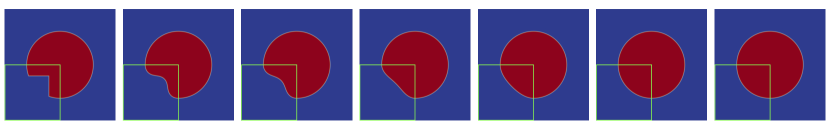
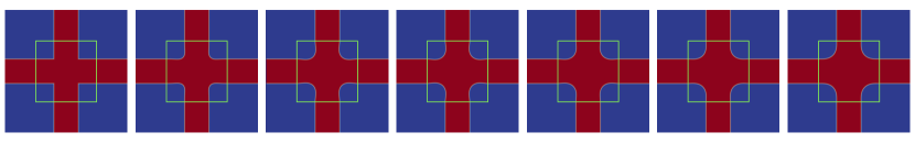
Figure 8: Application of our hybrid scheme to image restoration in two dimensions. In both examples, the spatial resolution is $n=1024$, the kernel size is $n_{K}=17$, and the interface parameter $\varepsilon=2^{-8}$ and the reconstruction region $D$ is outlined in green. In the top row, a disk with a cut-out corner is considered as initial image and we use $\tilde{\tau}=2^{-14}$, $\tau=2^{-7}$. The restoration evolution is shown at times $0,1,100,500,1000,1500$, and $2000$. In the bottom row, a cross shape is given as initial image with the central part is smoothed under discrete Willmore flow with stepsizes $\tilde{\tau}=2^{-14}$ and $\tau=2^{-14}$. We show the flow at times $0,1,5,10,20,35$, and $50$.

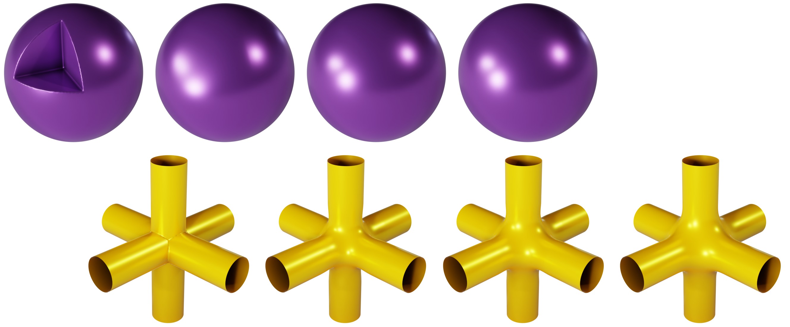
Figure 9: Application of our hybrid scheme to surface restoration in three dimensions. In both examples, the spatial resolution was $n=128$, the kernel size was $n_{K}=17$, the interface parameter was $\varepsilon=2^{-6}$, and the timestep sizes were $\tilde{\tau}=2^{-14}$ and $\tau=2^{-21}$. In the top row, the flow at timesteps $0,1,3$, and $5$ recovering a sphere with an initially cut-out corner is shown. In the bottom row, the flow at timesteps $0,1,4$, and $8$ leads to a smooth blending of six tubes.

6 Conclusions

In this paper, we presented a new hybrid scheme for Willmore flow in a phase field formulation, which combines a minimizing movement ansatz for the flow proposed by Franken et al. [26] with a neural operator approach to compute an approximation of the mean curvature following Bretin et al. [8]. For a fixed timestep size and scale parameter of the phase field ansatz, the hybrid scheme shows error reduction for increasing spatial resolution and stencil size of the network kernel. The new scheme comes with significantly reduced computing times. The resulting discrete Willmore flow properly reflects the qualitative behavior of the continuous flow and is, for instance, applicable to restoration of 2D images and 3D surfaces.

The results encourage the use of neural networks when simulating geometric flows. A future challenge would be to directly learn a solution operator for Willmore flow. In [28], Grzhibovskis and Heintz described a convolution thresholding scheme for Willmore flow. Hence, designing a neural network to directly learn Willmore flow does not seem to be out of reach. However, creating proper training data is more subtle. The striking observation in [8] is that the evolution of spheres under mean curvature flow is sufficient for the approximation of mean curvature flow for a wide range of initial data. For Willmore flow, surely a significantly richer set of training data is required.

Funding

This work was supported by the Deutsche Forschungsgemeinschaft (DFG, German Research Foundation) via project 211504053 – Collaborative Research Center 1060 and via Germany’s Excellence Strategy project 390685813 – Hausdorff Center for Mathematics. Furthermore, this project has received funding from the European Union’s Horizon 2020 research and innovation program under the Marie Skłodowska-Curie grant agreement No 101034255.

References

- [1] J. Ahrens, B. Geveci, and C. Law, ParaView: An end-user tool for large data visualization, in Visualization Handbook, Elsevier, 2005. ISBN 978-0123875822.
- [2] L. Ambrosio, N. Gigli, and G. Savaré, Gradient flows: in metric spaces and in the space of probability measures, Springer Science & Business Media, 2008.
- [3] N. Balzani and M. Rumpf, A nested variational time discretization for parametric Willmore flow, Interfaces and Free Boundaries, 14 (2013), pp. 431–454.
- [4] G. Barles and C. Georgelin, A simple proof of convergence for an approximation scheme for computing motions by mean curvature, SIAM Journal on Numerical Analysis, 32 (1995), pp. 484–500.
- [5] J. W. Barrett, H. Garcke, and R. Nürnberg, A parametric finite element method for fourth order geometric evolution equations, Journal of Computational Physics, 222 (2007), pp. 441–467.
- [6] Blender Online Community, Blender - a 3d modelling and rendering package, 2018.
- [7] A. I. Bobenko and P. Schröder, Discrete Willmore flow, in Proceedings of the Third Eurographics Symposium on Geometry Processing, SGP ’05, Goslar, DEU, 2005, Eurographics Association, pp. 101–es.
- [8] E. Bretin, R. Denis, S. Masnou, and G. Terii, Learning phase field mean curvature flows with neural networks, Journal of Computational Physics, 470 (2022), p. 111579.
- [9] E. Bretin, S. Masnou, and É. Oudet, Phase-field approximations of the Willmore functional and flow, Numerische Mathematik, 131 (2015), pp. 115–171.
- [10] J. Budd and Y. van Gennip, Graph Merriman–Bence–Osher as a Semi Discrete Implicit Euler Scheme for Graph Allen–Cahn Flow, SIAM Journal on Mathematical Analysis, 52 (2020), pp. 4101–4139.
- [11] F. Campelo, C. Arnarez, S. J. Marrink, and M. M. Kozlov, Helfrich model of membrane bending: From gibbs theory of liquid interfaces to membranes as thick anisotropic elastic layers, Advances in Colloid and Interface Science, 208 (2014), pp. 25–33. Special issue in honour of Wolfgang Helfrich.
- [12] P. G. Ciarlet, Mathematical Elasticity: Theory of Shells, Society for Industrial and Applied Mathematics, Philadelphia, PA, 2000.
- [13] U. Clarenz, U. Diewald, G. Dziuk, M. Rumpf, and R. Rusu, A finite element method for surface restoration with smooth boundary conditions, Computer Aided Geometric Design, 21 (2004), pp. 427–445.
- [14] K. Crane, U. Pinkall, and P. Schröder, Robust fairing via conformal curvature flow, ACM Transaction on Graphics, 32 (2013).
- [15] A. Dall’Acqua, M. Müller, R. Schätzle, and A. Spener, The willmore flow of tori of revolution, 2023.
- [16] E. De Giorgi, New problems on minimizing movements, Boundary Value Problems for PDE and Applications, (1993), p. 81–98.
- [17] K. Deckelnick and G. Dziuk, Error analysis of a finite element method for the Willmore flow of graphs., Interfaces and Free Boundaries, 8 (2006), pp. 21–46.
- [18] M. Desbrun, M. Meyer, P. Schröder, and A. H. Barr, Implicit fairing of irregular meshes using diffusion and curvature flow, in Proceedings of the 26th Annual Conference on Computer Graphics and Interactive Techniques, SIGGRAPH ’99, USA, 1999, ACM Press/Addison-Wesley Publishing Co., p. 317–324.
- [19] M. Droske and M. Rumpf, A level set formulation for Willmore flow, Interfaces and Free Boundaries, 6 (2004), pp. 361–378.
- [20] Q. Du, C. Liu, and X. Wang, A phase field approach in the numerical study of the elastic bending energy for vesicle membranes, Journal of Computational Physics, 198 (2004), pp. 450–468.
- [21] Q. Du and X. Wang, Convergence of numerical approximations to a phase field bending elasticity model of membrane deformations, International Journal of Numerical Analysis and Modeling, 4 (2007), pp. 441–459.
- [22] G. Dziuk, An algorithm for evolutionary surfaces, Numerische Mathematik, 58 (1991), pp. 603–611.
- [23] , Computational parametric Willmore flow, Numerische Mathematik, 111 (2008), pp. 55–80.
- [24] L. C. Evans, Convergence of an algorithm for mean curvature motion, Indiana University Mathematics Journal, 42 (1993), pp. 533–557.
- [25] R. Feinman, Pytorch-minimize: a library for numerical optimization with autograd, 2021.
- [26] M. Franken, M. Rumpf, and B. Wirth, A phase field based PDE constraint optimization approach to time discrete Willmore flow, International Journal of Numerical Analysis and Modeling, (2011).
- [27] A. Gruber and E. Aulisa, Computational p-willmore flow with conformal penalty, ACM Transaction on Graphics, 39 (2020).
- [28] R. Grzhibovskis and A. Heintz, A convolution thresholding scheme for the willmore flow, Interfaces and Free Boundaries, 10, pp. 139–153.
- [29] D. P. Kingma and J. Ba, Adam: A Method for Stochastic Optimization, in International Conference on Learning Representations, 2015.
- [30] M. Kleineberg, Mesh-to-sdf: Calculate signed distance fields for arbitrary meshes, 2021.
- [31] E. Kuwert and R. Schätzle, The Willmore flow with small initial energy, Journal of Differential Geometry, 57 (2001), pp. 409–441.
- [32] E. Kuwert and R. Schätzle, Gradient flow for the Willmore functional, Communications in Analysis and Geometry, 10 (2002), pp. 1228–1245 (electronic).
- [33] E. Kuwert and R. Schätzle, Removability of point singularities of Willmore surfaces, Annals of Mathematics, (2004), pp. 315–357.
- [34] S. Lee and Y. Choi, Curvature-based interface restoration algorithm using phase-field equations, Plos one, 18 (2023), p. e0295527.
- [35] F. C. Marques and A. Neves, Min-max theory and the Willmore conjecture, Annals of Mathematics, (2014), pp. 683–782.
- [36] B. Merriman, J. K. Bence, and S. J. Osher, Diffusion generated motion by mean curvature, CAM Report 92-18, University of California Los Angeles, 1992.
- [37] , Motion of multiple junctions: A level set approach, Journal of Computational Physics, 112 (1994), pp. 334–363.
- [38] L. Modica and S. Mortola, Un esempio di -convergenza, Boll. Un. Mat. Ital. B (5), 14 (1977), pp. 285–299.
- [39] M. Nitzberg, D. Mumford, and T. Shiota, Filtering, Segmentation and Depth (Lecture Notes in Computer Science Vol. 662), Springer-Verlag Berlin Heidelberg, 1993.
- [40] J. Nocedal and S. J. Wright, Numerical optimization, Springer Series in Operations Research and Financial Engineering, Springer, New York, second ed., 2006.
- [41] A. Paszke, S. Gross, F. Massa, A. Lerer, J. Bradbury, G. Chanan, T. Killeen, Z. Lin, N. Gimelshein, L. Antiga, A. Desmaison, A. Kopf, E. Yang, Z. DeVito, M. Raison, A. Tejani, S. Chilamkurthy, B. Steiner, L. Fang, J. Bai, and S. Chintala, Pytorch: An imperative style, high-performance deep learning library, in Advances in Neural Information Processing Systems, H. Wallach, H. Larochelle, A. Beygelzimer, F. d'Alché-Buc, E. Fox, and R. Garnett, eds., vol. 32, Curran Associates, Inc., 2019.
- [42] T. Rivière, Analysis aspects of Willmore surfaces, Inventiones Mathematicae, 174 (2008), pp. 1–45.
- [43] R. E. Rusu, An algorithm for the elastic flow of surfaces, Interfaces and Free Boundaries, 7 (2005), pp. 229–239.
- [44] O. Schenk, K. Gärtner, W. Fichtner, and A. Stricker, PARDISO: a high-performance serial and parallel sparse linear solver in semiconductor device simulation, Future Generation Computer Systems, 18 (2001), pp. 69–78. I. High Performance Numerical Methods and Applications. II. Performance Data Mining: Automated Diagnosis, Adaption, and Optimization.
- [45] H. Schumacher, On H2-gradient flows for the willmore energy, 2017.
- [46] G. Simonett, The Willmore Flow near spheres, Diff. and Integral Eq., 14(8) (2001), pp. 1005–1014.
- [47] Y. Soliman, A. Chern, O. Diamanti, F. Knöppel, U. Pinkall, and P. Schröder, Constrained willmore surfaces, ACM Transaction on Graphics, 40 (2021).
- [48] P. Virtanen, R. Gommers, T. E. Oliphant, M. Haberland, T. Reddy, D. Cournapeau, E. Burovski, P. Peterson, W. Weckesser, J. Bright, S. J. van der Walt, M. Brett, J. Wilson, K. J. Millman, N. Mayorov, A. R. J. Nelson, E. Jones, R. Kern, E. Larson, C. J. Carey, İ. Polat, Y. Feng, E. W. Moore, J. VanderPlas, D. Laxalde, J. Perktold, R. Cimrman, I. Henriksen, E. A. Quintero, C. R. Harris, A. M. Archibald, A. H. Ribeiro, F. Pedregosa, P. van Mulbregt, and SciPy 1.0 Contributors, SciPy 1.0: Fundamental Algorithms for Scientific Computing in Python, Nature Methods, 17 (2020), pp. 261–272.