Variance Reduction Methods Do Not Need to Compute Full Gradients: Improved Efficiency through Shuffling

Abstract

In today’s world, machine learning is hard to imagine without large training datasets and models. This has led to the use of stochastic methods for training, such as stochastic gradient descent (SGD). SGD provides weak theoretical guarantees of convergence, but there are modifications, such as Stochastic Variance Reduced Gradient (SVRG) and StochAstic Recursive grAdient algoritHm (SARAH), that can reduce the variance. These methods require the computation of the full gradient occasionally, which can be time consuming. In this paper, we explore variants of variance reduction algorithms that eliminate the need for full gradient computations. To make our approach memory-efficient and avoid full gradient computations, we use two key techniques: the shuffling heuristic and idea of SAG/SAGA methods. As a result, we improve existing estimates for variance reduction algorithms without the full gradient computations. Additionally, for the non-convex objective function, our estimate matches that of classic shuffling methods, while for the strongly convex one, it is an improvement. We conduct comprehensive theoretical analysis and provide extensive experimental results to validate the efficiency and practicality of our methods for large-scale machine learning problems.

1 Introduction

In recent years, machine learning has experienced remarkable progress. It has been driven by the pursuit of enhanced performance and the ability to tackle increasingly complex challenges, which have become central focuses for researchers and engineers alike. This focus has led to a substantial expansion in both the volume of data samples and the scale of models. These development is crucial, as it contributes to greater result stability and enhanced overall task performance. The majority of machine learning tasks are based on the finite-sum minimization problem:

$$\underset{x\in\mathbb{R}^{d}}{\min}\left[f(x)=\frac{1}{n}\sum\nolimits_{i=1}^{n}f_{i}(x)\right],$$ (1)

where $f_{i}:\mathbb{R}^{d}\rightarrow\mathbb{R}$ and the number of functions $n$ is large. To illustrate, in the context of training machine learning models, let $n$ represent the size of the training set and $f_{i}(x)$ denote the loss of the model on the $i$-th data point, where $x$ is the vector of model parameters.

Stochastic methods are especially suitable for this problem because they can avoid calculating the full gradient at each algorithm iteration. This is because such an action is prohibitively expensive in real-world learning problems due to the large values of $n$. One of the most well-known stochastic methods for solving this problem is SGD (Robbins and Monro, 1951; Moulines and Bach, 2011) and its multiple modifications (Lan, 2020). At iteration $t$, the algorithm selects a single index $i_{t}$ from the set $\{1,\ldots,n\}$ and performs the following step with the stepsize $\gamma$.

$$x^{t+1}=x^{t}-\gamma\nabla f_{i_{t}}(x^{t}).$$

$\bullet$ Variance reduction technique. Despite the simplicity of classical SGD and the fact that its properties and evaluation are deeply studied, it has one significant drawback: the classical variance of its native stochastic estimators of full gradients remains large throughout the learning process. Thus, SGD with constant learning rate converges linearly only to the neighborhood of the optimal solution, the size of which is proportional to the step and variance (Gower et al., 2020). Fortunately, the technique of variance reduction (VR) (Johnson and Zhang, 2013) was proposed to address this issue. Some of the most popular methods based on this technique are SVRG (Johnson and Zhang, 2013), SARAH (Nguyen et al., 2017; Hu et al., 2019), SAG (Roux et al., 2012), SAGA (Defazio et al., 2014a), Finito (Defazio et al., 2014b), SPIDER (Fang et al., 2018). In this paper, we analyze two of these algorithms: Stochastic Variance Reduced Gradient (SVRG) and StochAstic Recursive grAdient algoritHm (SARAH). Let us start with SVRG that comprises the following steps:

$$\begin{split}&v^{t}=\nabla f_{i_{t}}(x^{t})-\nabla f_{i_{t}}(\omega^{t})+\nabla f(\omega^{t}),\\ &x^{t+1}=x^{t}-\gamma v^{t},\end{split}$$ (2)

where index $i_{t}$ is selected at the $t$-th iteration. Let us pay attention to the reference point $\omega^{t}$. This point should be updated periodically, either after a fixed number of iterations (e.g., once per epoch) or randomly (as in loopless versions; see (Kovalev et al., 2020)). The goal of update mechanisms like (2) is to move beyond the limitations of naive gradient estimators. It employs an iterative process to construct and apply a gradient estimator whose variance is progressively diminished. This approach allows for the safe use of larger learning rates, thereby accelerating the training process. Now let us look at another approach, SARAH, which updates the estimator of the full gradient recursively:

$$\begin{split}&v^{t}=\nabla f_{i_{t}}(x^{t})-\nabla f_{i_{t}}(x^{t-1})+v^{t-1},\\ &x^{t+1}=x^{t}-\gamma v^{t}.\end{split}$$ (3)

The problem with this procedure is that it fails to converge to the optimal solution $x^{*}$. To resolve this, we need to periodically update $v^{t}$ using the full gradient. Like SVRG, this process restarts after either a fixed number of iterations or randomly (Li et al., 2020). Furthermore, there is a practical version of SARAH that surpasses the performance of SVRG. In that version, the idea of the automatic choice of iterations to update the full gradient estimation is applied by computing the ratio $\frac{\|v^{t}\|}{\|v^{0}\|}$ (SARAH+ (Nguyen et al., 2017)).

$\bullet$ Shuffling heuristic. Now let us present an heuristic for selecting the $i_{t}$-th indexes at each iteration of the algorithms. Note that a comprehensive examination of such approaches has a potential to result in the development of more stable and efficient algorithms. In this paper, we utilize the shuffling heuristic (Bottou, 2009; Mishchenko et al., 2020; Safran and Shamir, 2020), which plays a crucial role in our algorithms. The technique is as follows: rather than selecting the index $i_{t}$ randomly and independently at each iteration, as in classical stochastic methods, we take a more practical approach. We first permute the sequence of indexes ${1,\ldots,n}$ and then select an index based on its position in this permutation during and epoch. There is a number of different shuffling techniques. Some of the most popular approaches include Random Reshuffle (RR), which involves shuffling data before each epoch, Shuffle Once (SO), which shuffles data once at the beginning of training, and Cyclic Permutation, which accesses data deterministically in a cyclic manner In our study, we do not explore the differences between these approaches; instead, we highlight one important common property among them: during one epoch, we calculate the stochastic gradient for each data sample exactly once. Let us formalize this setting. At each epoch $s$, we have a set of indexes $\{\pi_{s}^{0},\pi_{s}^{1},\ldots,\pi_{s}^{n-1}\}$ that is a random permutation of the set $\{0,1,\ldots,n-1\}$. Then, e.g. the SVRG update (2) of the full gradient estimator at the $t$-th iteration of this epoch transforms into

$$v^{t}=\nabla f_{\pi_{s}^{t}}(x_{s}^{t})-\nabla f_{\pi_{s}^{t}}(\omega^{t})+\nabla f(\omega^{t}).$$

Nevertheless, the analysis of shuffling methods has some specific details. The key difference between shuffling and independent choice is that shuffling methods do not have one essential property – the unbiasedness of stochastic gradients derived from the i.i.d. sampling:

$$\mathbb{E}_{\pi_{s}^{t}}\left[\nabla f_{\pi_{s}^{t}}(x_{s}^{t})\right]\neq\frac{1}{n}\sum\nolimits_{i=1}^{n}\nabla f_{\pi_{s}^{i}}(x)=\nabla f(x).$$

This restriction leads to a more complex analysis and non-standard techniques for proving the shuffling methods.

2 Brief literature review

$\bullet$ No full gradient methods. SVRG (2) and SARAH (3) are now the standard choices for solving a finite sum problem. Nevertheless, they suffer from one significant drawback – the necessity for the full gradient computation of the target function. There is considerable interest in variance reduction methods that avoid calculating full gradients. While SAG (Roux et al., 2012) and SAGA (Defazio et al., 2014a) address this issue, they necessitate substantial additional memory allocation, with a complexity of $\mathcal{O}(nd)$. Separately, it is worth noting the attempts to remove the computation of the full gradient in SARAH. First approach was supposed by (Nguyen et al., 2021). The authors proposed inexact SARAH algorithm, where computation of the full gradient obviates with mini-batch gradient estimate $\frac{1}{|S|}\sum_{i\in S}f_{i}(x),S\subset\{1,\ldots,n\}$. To converge to the point with $\varepsilon$-accuracy, this algorithm needs the batch size $|S|\sim\mathcal{O}\left(\frac{1}{\varepsilon}\right)$ and the stepsize $\gamma\sim\mathcal{O}\left(\frac{\varepsilon}{L}\right)$. Another approach actively uses the recursive SARAH update of the full gradient estimator and in the set of works authors proposed the following hybrid scheme without any restarts:

$$v^{t}=\beta_{t}\nabla f_{i_{t}}(x^{t})+(1-\beta_{t})(\nabla f_{i_{t}}(x^{t})-\nabla f_{i_{t}}(x^{t-1})+v^{t-1}).$$

In the work (Liu et al., 2020), it is used with constant parameter $\beta_{t}=\beta$, the STORM method (Cutkosky and Orabona, 2019) considers $\beta_{t}$ decreasing to zero and ZeroSARAH (Li et al., 2021) combines it with SAG/SAGA. Now let us take a look on the approaches that build methods without computing the full gradient in combination with shuffling techniques, since it is of particular interest in the context of our work. There is a list of works in which research has been conducted in this direction. Methods IAG (Gurbuzbalaban et al., 2017), PIAG (Vanli et al., 2016), DIAG (Mokhtari et al., 2018), SAGA (Park and Ryu, 2020; Ying et al., 2020), Prox-DFinito (Huang et al., 2021) naively store stochastic gradients and even PIAG, DIAG, Prox-DFinito that provide the best oracle complexity for the methods with shuffling heuristic from the current state of the theory , still require $\mathcal{O}(nd)$ of extra memory that is suboptimal in the large-scale problems. Methods AVRG (Ying et al., 2020) and the modification of SARAH (Beznosikov and Takáč, 2023) eliminates this issue, however, it deteriorates the oracle complexity. Thus, there are still no variance reduction methods that obviate the need for computing full gradients and are optimal in terms of additional memory and acceptable oracle complexity. We, in turn, address this gap.

$\bullet$ Shuffling methods. As our methods utilize a shuffling heuristic, we will review existing general shuffling techniques and compare their complexity to ours. Conceptually, the use of shuffling techniques has been a focus of research attention for a long time. In fact, sampling without replacement in finite-sum problems guarantees that within a single epoch, we account for the gradient of every function precisely once. It has been also demonstrated that Random Reshuffle converges more rapidly than SGD on a multitude of practical tasks (Bottou, 2009; Recht and Ré, 2013).

Nevertheless, the theoretical estimates of shuffling methods remained significantly worse than the theoretical estimates of SGD-like methods (Rakhlin et al., 2012; Drori and Shamir, 2020; Nguyen et al., 2019). A breakthrough was the work (Mishchenko et al., 2020) which presented new proof techniques and approaches to understanding shuffling. In particular, the results for strongly convex problems coincided with the results of SGD with an independent choice of indexes (Moulines and Bach, 2011; Stich, 2019). However, in the non-convex case, the results themselves were inferior to those of SGD with an independent choice index selection (Ghadimi and Lan, 2013). Furthermore, the major problem was the requirement for a large number of epochs to obtain convergence estimates in the non-convex case. This requirement is unnatural for real modern neural networks, where models are trained on a fairly small number of epochs. The solution of this problem was presented in the work (Koloskova et al., 2024). The authors built their analysis on the basis of convergence over a shorter period, called the correlation period, rather than on the basis of convergence over one epoch. This offers a more rigorous assessment and provides a foundation for future research.

In all these works, the shuffling heuristic was considered in relation to vanilla SGD, which is not an optimal method for the finite-sum problem under consideration (Zhang et al., 2020; Allen-Zhu, 2018) and generally speaking is out of the scope of this paper. The research was also continued in a more general formulation of the problem as variational inequalities (Beznosikov et al., 2023). Thus, (Medyakov et al., 2024) applied a shuffling heuristic to the Extragradient method (Juditsky et al., 2011) and achieved a similar estimate in a linear term with that for the method without shuffling. Consequently, researchers directed their attention to the shuffling heuristic in conjunction with the variance reduction methods and have obtained linear convergence of the methods. Most of all, the SVRG method was investigated. The first theoretical guarantees for the Extragradient method with the variance reduction scheme was obtained in (Medyakov et al., 2024), who succeeded in obtaining a linear convergence estimate for methods with shuffling in the VI problem. In the case of the finite-sum minimization, we pay spacial attention on the works (Malinovsky et al., 2023; Sun et al., 2019). But the theoretical estimates in these papers are still far from the estimates of the methods with an independent choice of indexes (Allen-Zhu and Hazan, 2016). As for this paper, we improve the estimates in the case of a strongly convex objective.

The convergence results from the mentioned and other works are presented in Table 1. One can observe that we compare our results only with studies using a shuffling setting where linear convergence was achieved.

Algorithm	No Full Grad.?	Memory	Non-Convex	Strongly Convex
SAGA Park and Ryu (2020)	✓	$\mathcal{O}(nd)$	$\backslash$	$\mathcal{O}\left(n\frac{L^{\color[rgb]{0.75390625,0.18359375,0.09765625}{2}}}{\mu^{\color[rgb]{0.75390625,0.18359375,0.09765625}{2}}}\log\left(\frac{1}{\varepsilon}\right)\right)$
IAG Gurbuzbalaban et al. (2017)	✓	$\mathcal{O}(nd)$	$\backslash$	$\mathcal{O}\left(n^{\color[rgb]{0.75390625,0.18359375,0.09765625}{2}}\frac{L^{\color[rgb]{0.75390625,0.18359375,0.09765625}{2}}}{\mu^{\color[rgb]{0.75390625,0.18359375,0.09765625}{2}}}\log\left(\frac{1}{\varepsilon}\right)\right)$
PIAG Vanli et al. (2016)	✓	$\mathcal{O}(nd)$	$\backslash$	$\mathcal{O}\left(n\frac{L}{\mu}\log\left(\frac{1}{\varepsilon}\right)\right)$
DIAG Mokhtari et al. (2018)	✓	$\mathcal{O}(nd)$	$\backslash$	$\mathcal{O}\left(n\frac{L}{\mu}\log\left(\frac{1}{\varepsilon}\right)\right)$
Prox-DFinito Huang et al. (2021)	✓	$\mathcal{O}(nd)$	$\backslash$	$\mathcal{O}\left(n\frac{L}{\mu}\log\left(\frac{1}{\varepsilon}\right)\right)$
AVRG Ying et al. (2020)	✓	$\mathcal{O}(d)$	$\backslash$	$\mathcal{O}\left(n\frac{L^{\color[rgb]{0.75390625,0.18359375,0.09765625}{2}}}{\mu^{\color[rgb]{0.75390625,0.18359375,0.09765625}{2}}}\log\left(\frac{1}{\varepsilon}\right)\right)$
SVRG Sun et al. (2019)	✗	$\mathcal{O}(d)$	$\backslash$	$\mathcal{O}\left(n^{\color[rgb]{0.75390625,0.18359375,0.09765625}{3}}\frac{L^{\color[rgb]{0.75390625,0.18359375,0.09765625}{2}}}{\mu^{\color[rgb]{0.75390625,0.18359375,0.09765625}{2}}}\log\left(\frac{1}{\varepsilon}\right)\right)$
SVRG Malinovsky et al. (2023)	✗	$\mathcal{O}(d)$	$\mathcal{O}\left(\frac{nL}{\varepsilon^{2}}\right)$	$\mathcal{O}\left(n\frac{L^{\color[rgb]{0.75390625,0.18359375,0.09765625}{\nicefrac{{3}}{{2}}}}}{\mu^{\color[rgb]{0.75390625,0.18359375,0.09765625}{\nicefrac{{3}}{{2}}}}}\log\left(\frac{1}{\varepsilon}\right)\right)^{\color[rgb]{0.75390625,0.18359375,0.09765625}{\text{(1)}}}$
SARAH Beznosikov and Takáč (2023)	✓	$\mathcal{O}(d)$	$\backslash$	$\mathcal{O}\left(n^{\color[rgb]{0.75390625,0.18359375,0.09765625}{2}}\frac{L}{\mu}\log\left(\frac{1}{\varepsilon}\right)\right)$
SVRG (Algorithm 1 in this paper)	✓	$\mathcal{O}(d)$	$\mathcal{O}\left(\frac{nL}{\varepsilon^{2}}\right)$	$\mathcal{O}\left(n\frac{L}{\mu}\log\left(\frac{1}{\varepsilon}\right)\right)$
SARAH (Algorithm 1 in this paper)	✓	$\mathcal{O}(d)$	$\mathcal{O}\left(\frac{nL}{\varepsilon^{2}}\right)$	$\mathcal{O}\left(n\frac{L}{\mu}\log\left(\frac{1}{\varepsilon}\right)\right)$

Table 1: Comparison of the convergence results.

• Columns: No Full Grad.? = whether the method computes full gradients, Memory = amount of additional memory.

• Notation: $\mu$ = constant of strong convexity, $L$ = smoothness constant, $n$ = size of the dataset, $d$ = dimension of the problem, $\varepsilon$ = accuracy of the solution.

• (1): In this work, there are also improved results that hold in the big data regime: $n\gg\mathcal{O}\left(\frac{L}{\mu}\right)$, but it is out of the scope of this work.

3 Contributions

Our contributions are as follows.

$\bullet$ Full gradient approximation. We explore an approach whose key feature is approximating the full gradient of the objective function using a shuffling heuristic (Beznosikov and Takáč, 2023). Moreover, this method does not require any additional $\mathcal{O}(nd)$ memory. Instead, we iteratively build the approximation over an epoch.
$\bullet$ No need to compute full gradient in variance reduction algorithms. In a sense, we construct a universal analysis for our gradient approximation and it allows us to equally apply it to two variance reduction methods:

• Classical SVRG (Johnson and Zhang, 2013),

• SARAH in the closest form to one in (Beznosikov and Takáč, 2023), however, we transform their algorithm to improve convergence estimates.

$\bullet$ Convergence results. We obtain convergence results under different assumptions on the objective function. We consider the non-convex case, which is of the greatest interest in modern machine learning problems, as well as the strongly convex case. We obtain state-of-the-art guarantees of convergence in the class of variance reduction algorithms, that do not need the computation of the full gradient at all, for both of our methods. Additionally, we improve upper estimate of shuffling methods in the strongly convex case.
$\bullet$ Experiments. We conduct experiments on specific tasks and compare the performance of the considered methods.

4 Assumptions

We provide a list of assumptions below.

Assumption 1.

Each function $f_{i}$ is $L$-smooth, i.e., it satisfies $\|\nabla f_{i}(x)-\nabla f_{i}(y)\|\leq L\|x-y\|$ for any $x,y\in\mathbb{R}^{d}$.

Assumption 2.

1. Strong Convexity: Each function $f_{i}$ is $\mu$-strongly convex, i.e., for any $x,y\in\mathbb{R}^{d}$, it satisfies

   $$f_{i}(y)\geqslant f_{i}(x)+\langle\nabla f_{i}(x),y-x\rangle+\frac{\mu}{2}\|y-x\|^{2}.$$

2. Non-Convexity: The function $f$ has a (may be not unique) finite minimum, i.e. $f^{*}=\inf\limits_{x\in\mathbb{R}^{d}}f(x)>-\infty$.

5 Algorithms and convergence analysis

5.1 Full gradient approximation

In this section, we introduce an approach based on the shuffling heuristic and SAG/SAGA ideas that not only approximates the full gradient, but also optimizes memory usage by avoiding the storage of past gradient values.

The SAG algorithm is one of the early methods designed to improve the convergence speed of stochastic gradient methods by reducing the variance of gradient updates. In SAG, the update step can be written as

(4)

where $\phi_{j}^{t}$ represents the past iteration at which the gradients for the $j$-th function are considered. The core idea is that we store old gradients for each function (essentially storing gradients $\nabla f_{j}(\phi_{j})$ rather than points $\phi_{j}$), and at each iteration, we update one component of this sum with a newly computed gradient.

In SAG, $i_{t}$ are sampled independently at each iteration, which makes it unclear when the gradient for a specific index was last computed. However, in the case of shuffling, we know that during an epoch, the gradient for each $\nabla f_{j}$ is computed. Thus, at the beginning of an epoch, we reliably approximate the gradient in the same way as in SAG:

$$\textstyle{v_{s+1}=\frac{1}{n}\sum_{t=1}^{n}\nabla f_{\pi_{s}^{t}}(x_{s}^{t}),}$$ (5)

where $\pi_{s}^{t}$ denotes the sequence of data points after shuffling at the beginning of epoch $s$. This computation is done without additional memory, using a simple moving average during the previous epoch:

$$\begin{split}\quad~~~&\textstyle{\widetilde{v}_{s}^{t+1}}=\textstyle{\frac{t}{t+1}\widetilde{v}_{s}^{t}+\frac{1}{t+1}\nabla f_{\pi_{s}^{t}}(x_{s}^{t})},\\ \quad~~~&v_{s+1}=\widetilde{v}_{s}^{n}.\end{split}$$ (6)

It is a simple exercise to prove (6) matches (5) and we show it in the proof of Lemma 2.

5.2 SVRG without full gradients

As we already mentioned, variance reduced methods suffer from the major obstacle — they have to compute the full gradient once at each epoch or use additional memory of a larger size. To address this limitation, in this section, we propose a novel algorithm, based on the classical SVRG that not only eliminates the need for full gradient computation but also optimizes memory usage by avoiding the storage of past gradient values.

Previously, in Section 5.1, we defined the way we can approximate the full gradient: (5), (6). However, this approach introduces a question: how should we alter and use the gradient approximation $v_{s}$ throughout an epoch? In SAG (4), we added a new $\nabla f_{i_{t}}(x^{t})$ and removed its old version $\nabla f_{i_{t}}(\phi_{i_{t}}^{t})$, but this requires memory for all $\nabla f_{i_{t}}$ ($\phi_{i_{t}}^{t}$). Building on the concept from SVRG (2), rather than computing $\nabla f_{i_{t}}$ ($\phi_{i_{t}}^{t}$), our update uses the gradient at a reference point $\omega_{s}$. Unlike SVRG, which uses the full gradient at this reference point as shown in (2), we use an approximation provided by (5):

$$v_{s}^{t} =\nabla f_{\pi_{s}^{t}}(x_{s}^{t})-\nabla f_{\pi_{s}^{t}}(\omega_{s})+v_{s}.$$

Finally, we do the step of the algorithm in Line 9, where the approximation $v_{s}$ is calculated in the previous epoch as (6) in Line 7. We now present the formal description of No Full Grad SVRG (Algorithm 1).

Algorithm 1 No Full Grad SVRG

1:Input: Initial points $x_{0}^{0}\in\mathbb{R}^{d},\omega_{0}=x_{0}^{0}$; Initial gradients $\widetilde{v}_{0}^{0}=0^{d},v_{0}=0^{d}$

2:Parameter: Stepsize $\gamma>0$

3:for epochs $s=0,1,2,\ldots,S$ do

4:  Sample a permutation $\pi^{0}_{s},\dots,\pi^{n-1}_{s}$ of $\overline{0,n-1}$

5:              // Sampling depends on shuffling heuristic

6:  for $t=0,1,2,\ldots,n-1$ do

7:    $\widetilde{v}_{s}^{t+1}=\frac{t}{t+1}\widetilde{v}_{s}^{t}+\frac{1}{t+1}\nabla f_{\pi_{s}^{t}}(x_{s}^{t})$

8:    $v_{s}^{t}=\nabla f_{\pi_{s}^{t}}(x_{s}^{t})-\nabla f_{\pi_{s}^{t}}(\omega_{s})+v_{s}$

9:    $x_{s}^{t+1}=x_{s}^{t}-\gamma v_{s}^{t}$

10:  end for

11:  $x_{s+1}^{0}=x_{s}^{n}$

12:   $\omega_{s+1}=x_{s}^{n}$

13:   $\widetilde{v}_{s+1}^{0}=0^{d}$

14:  $v_{s+1}=\widetilde{v}_{s}^{n}$

15:end for

The outstanding issue is selecting the point $\omega_{s}$ (Line 12). The approximation $v_{s}$, representing the full gradient at $\omega_{s}$, is derived from gradients evaluated at points between $x_{s-1}^{1}$ and $x_{s-1}^{n}$. A reasonable choice for $\omega_{s}$ seems to be the average of these points. However, during this epoch, we are continuously moving away from this point, computing $\nabla f_{\pi_{s}^{t}}(x_{s}^{t})$ and adding to the reduced gradient. Consequently, the average point changes over time. By the end of the current epoch, it evolves into an average calculated from points ranging from $x_{s}^{1}$ to $x_{s}^{n}$. Thus, choosing $\omega_{s}$ as the last point from the previous epoch is a logical compromise, since we estimate not only how far we can move during the past epoch but also how far we have moved during the current one (see Lemma 1). An intriguing question for future research is whether more frequent or adaptive updates of $\omega_{s}$ could further improve convergence rates (Allen-Zhu and Hazan, 2016).

By integrating this dynamic strategy, our approach not only improves the efficiency of gradient updates but also optimizes memory usage, making it suitable for large-scale optimization problems. Now let us move to the theoretical analysis. We consider the problem in two formulations: in the non-convex and strongly convex cases.

5.2.1 Non-convex setting

For a more detailed analysis of this method, let us examine the interim results. We structure our analysis as follows: first, we analyze convergence over a single epoch, and then we extend this analysis recursively across all epochs. The crucial aspect here is understanding how gradients change from the start to different points within an epoch. To begin with, we need to show that these changes depend on two critical factors: first, how well we approximate the true full gradient at the start of each epoch; second, how far our updates stray from this initial reference point as we move through it. To obtain this, we present a lemma.

Lemma 1.

Suppose Assumptions 1, 2 hold. Then for Algorithm 1 a valid estimate is

$$\left\|\nabla f(\omega_{s})-\frac{1}{n}\sum\nolimits_{t=0}^{n-1}v_{s}^{t}\right\|^{2}\hskip-2.84526pt\leqslant ~~2\|\nabla f(\omega_{s})-v_{s}\|^{2}$$

$$+\frac{2L^{2}}{n}\sum\nolimits_{t=0}^{n-1}\|x_{s}^{t}-\omega_{s}\|^{2}.$$

In contrast to classical SVRG, where only one term matters due to exact computation of full gradients ($v_{s}=\nabla f(\omega_{s})$), our algorithm avoids such computations. Instead, it introduces an additional term representing errors in approximating these gradients. This error fundamentally reflects discrepancies between our approximation and actual gradients at $\omega_{s}$. Given that $v_{s}$ averages stochastic gradients from previous epochs (as per Equation (5)) with $\omega_{s}$ set as their final point, this error quantifies shifts among those points relative to future reference points. Thus, beginning each epoch at $\omega_{s}$, we gauge both potential movement within upcoming epochs and progress made during past ones. This perspective underscores a strategic balance involved when selecting $\omega_{s}$, aligning with discussions found in Section 5.2. We now present estimates for these deviations through a subsequent lemma.

Lemma 2.

Suppose Assumptions 1, 2 hold. Let the stepsize $\gamma\leqslant\frac{1}{2Ln}$. Then for Algorithm 1 a valid estimate is

$$\left\|\nabla f(\omega_{s})-\frac{1}{n}\sum\nolimits_{t=0}^{n-1}v_{s}^{t}\right\|^{2} \leqslant 8\gamma^{2}L^{2}n^{2}\|v_{s}\|^{2}$$

$$+32\gamma^{2}L^{2}n^{2}\|v_{s-1}\|^{2}.$$

Now we are ready to present the final result of this section.

Theorem 1.

Suppose Assumptions 1, 2(b) hold. Then Algorithm 1 with $\gamma\leqslant\frac{1}{20Ln}$ to reach $\varepsilon$-accuracy, where $\varepsilon^{2}=\frac{1}{S}\sum\nolimits_{s=1}^{S}\|\nabla f(\omega_{s})\|^{2}$, needs

$$\mathcal{O}\left(\frac{nL}{\varepsilon^{2}}\right)~~\text{iterations and oracle calls.}$$

Detailed proofs of the results obtained can be found in Appendix, Section C. Let us delve into the result of this theorem. We obtained the first variance reduction method without calculating the full gradient and optimal on additional memory in the non-convex setting. Our results showed that the score is by an order of magnitude inferior, compared to the classical SVRG using independent sampling: $\mathcal{O}(nL)$ versus $\mathcal{O}(n^{\nicefrac{{2}}{{3}}}L)$ (Allen-Zhu and Hazan, 2016). In a sense, this is payback for the fact that we approximate the full gradient at the reference point, rather than considering at the current state. As for the Shuffle SVRG, we replicate the current optimal estimate (Malinovsky et al., 2023). Taking into account that our method does not require the calculation of full gradients at all, it is valid and worth considering for the further research. Finally, the development of no-full-grad option for non-convex problems is a strong contribution, as this area has not been extensively explored before (Table 1).

5.2.2 Strongly convex setting

Let us analyze this algorithm for the strongly convex case. Based on the proof of Theorem 1, we can construct an analysis for strongly convex setting, actively using Polyak-Lojasiewicz condition (see Appendix, Section B). In that way, we present the following guarantees of convergence.

Theorem 2.

Suppose Assumptions 1, 2(a) hold. Then Algorithm 1 with $\gamma\leqslant\frac{1}{20Ln}$ to reach $\varepsilon$-accuracy, where $\varepsilon=f(\omega_{S+1})-f(x^{*})$, needs

$$\mathcal{O}\left(\frac{nL}{\mu}\log\frac{1}{\varepsilon}\right)~~\text{iterations and oracle calls.}$$

Our results for the No Full Grad SVRG algorithm under strong convexity conditions are similar to those observed in non-convex settings. Furthermore, it is much better, than currently available estimates of no-full-grad methods. When comparing our results to those of other shuffling methods (as shown in Table 1), it is evident that our algorithm improves convergence guarantees, while keeping optimal extra memory. In that way, it is a contribution to the whole class of shuffling algorithms.

5.3 SARAH without full gradients

We have earlier discussed that SARAH was designed as the variance reduction method, which outperforms SVRG on practice and has a lot of interesting practical applications (Nguyen et al., 2017). It would be a great omission on our part not to do an analysis for this method. This section discusses how to modify the SARAH method to avoid restarts. We consider two approaches: taking steps based on an accurate full gradient or developing a version of SARAH that does not require full gradient computations.

There also exists a version of SARAH, that obviates the need of the full gradient computation (Beznosikov and Takáč, 2023), however its upper estimate, $\mathcal{O}\left(n^{2}\frac{L}{\mu}\log\left(\frac{1}{\varepsilon}\right)\right)$, is far from the one we obtain for SVRG in the previous section. Let us show what we can change in their method to improve this estimate. The authors in the mentioned work used the same technique to approximate the full gradient as (5). The algorithm used the standard SARAH update formula (3) throughout each epoch. To initiate a new recursive cycle at the start of every epoch, an extra step was taken with an approximated full gradient. In this way, they also used the SAG/SAGA idea but provided a recursive reduced gradient update to avoid storing all stochastic gradients during the epoch.

To continue the analysis, we want to shade some light on the differences between SAG and SAGA algorithms, since it is crucial for our modifications. We have already discussed the SAG update (4). The SAGA update is almost the same, except for the absent factor $\frac{1}{n}$. Thus, maintaining the notation we used for SAG, we can write the SAGA step as

(7)

The key difference hides in the reduction of the variance of the SAG update in $n^{2}$ times compared to SAGA with the same $\phi$’s, however, the payback for such a gain is a non-zero bias in SAG. The choice towards unbiasedness of reduced operators was made in SAGA mainly in order to obtain a simple and tight theory for variance reduction methods and to yield theoretical estimates for proximal operators (Defazio et al., 2014a).

Now we can specify and say that the idea behind SAGA was applied in (Beznosikov and Takáč, 2023). Nevertheless, attempting to increase variance for the sake of zero bias appears illogical here because the shuffling heuristic remains in use, thereby inherently introducing bias. As a result, achieving convergence requires very small step sizes, leading to significantly worse estimates. In contrast, we propose leveraging the concept of SAG, similar to what we did in No Full Grad SVRG, and modifying the SARAH update during each epoch, as

$$v_{s}^{t+1} =\frac{1}{n}\left(\nabla f_{\pi_{s}^{t}}(x_{s}^{t})-\nabla f_{\pi_{s}^{t}}(x_{s}^{t-1})\right)+v_{s}^{t-1}.$$

This helps us to safely use bigger steps and improve convergence rates. We provide the formal description of the No Full Grad SARAH method (Algorithm 2).

Algorithm 2 No Full Grad SARAH

1:Input: Initial points $x_{0}^{0}\in\mathbb{R}^{d}$; Initial gradients $\widetilde{v}_{0}^{0}=0^{d},v_{0}=0^{d}$

2:Parameter: Stepsize $\gamma>0$

3:for epochs $s=0,1,2,\ldots,S$ do

4:  Sample a permutation $\pi^{1}_{s},\dots,\pi^{n}_{s}$ of $\overline{1,n}$

5:          // Sampling depends on shuffling heuristic

6:  $v_{s}^{0}=v_{s}$

7:  $x_{s}^{1}=x_{s}^{0}-\gamma v_{s}^{0}$

8:  for $t=1,2,3,\ldots,n$ do

9:    $\widetilde{v}_{s}^{t+1}=\frac{t-1}{t}\widetilde{v}_{s}^{t}+\frac{1}{t}\nabla f_{\pi_{s}^{t}}(x_{s}^{t})$

10:    $v_{s}^{t}=\frac{1}{n}\left(\nabla f_{\pi_{s}^{t}}(x_{s}^{t})-\nabla f_{\pi_{s}^{t}}(x_{s}^{t-1})\right)+v_{s}^{t-1}$

11:    $x_{s}^{t+1}=x_{s}^{t}-\gamma v_{s}^{t}$

12:  end for

13:  $x_{s+1}^{0}=x_{s}^{n+1}$

14:   $\widetilde{v}_{s+1}^{1}=0^{d}$

15:  $v_{s+1}=\widetilde{v}_{s}^{n+1}$

16:end for

One can observe that we slightly modify the coefficients in the full gradient approximation scheme (Line 9 of Algorithm 2) compared to Algorithm 1. The discrepancy stems solely from differences in indexing. In this case, the full gradient approximation begins at iteration $t=1$ rather than $t=0$, as we incorporate an extra restart step not present in SVRG. Therefore, to prevent the factor from becoming $\frac{1}{n+1}$ instead of $\frac{1}{n}$ in (5), we make this adjustment. Now we proceed to the theoretical analysis of Algorithm 2 under both non-convex and strongly convex assumptions on the objective function.

5.3.1 Non-convex setting

During the proof of SARAH’s convergence estimates, we proceed analogously to how we did for SVRG. Initially, we focus on a single epoch and demonstrate convergence within it. To achieve this, we estimate the difference between the gradient at the start of the epoch and the average of reduced gradients used for updates throughout that epoch.

Lemma 3.

Suppose that Assumptions 1, 2 hold. Then for Algorithm 2 a valid estimate is

$$\textstyle{\left\|\nabla f(x_{s}^{0})-\frac{1}{n+1}\sum\nolimits_{t=0}^{n}v_{s}^{t}\right\|^{2}\leqslant} \textstyle{~2\|\nabla f(x_{s}^{0})-v_{s}\|^{2}}$$

$$\textstyle{\hskip-2.84526pt+\frac{2L^{2}}{n+1}\sum\nolimits_{t=1}^{n}\|x_{s}^{t}-x_{s}^{t-1}\|^{2}.}$$

The first term is identical to the one we previously encountered in the analysis of Algorithm 1: the difference between the true full gradient and its approximation. Additionally, note that the second term conveys a similar meaning to its counterpart in Lemma 1, representing the difference between current and reference points during an epoch (where the reference point is consistently set as the previous one). In that way, we proceed analogically to SVRG and move to the following lemma.

Lemma 4.

Suppose that Assumptions 1, 2 hold. Let the stepsize $\gamma\leqslant\frac{1}{3L}$. Then for Algorithm 2 a valid estimate is

$$\left\|\nabla f(x_{s}^{0})-\frac{1}{n+1}\sum\nolimits_{t=0}^{n}v_{s}^{t}\right\|^{2} \leqslant 9\gamma^{2}L^{2}\|v_{s}\|^{2}$$

$$+36\gamma^{2}L^{2}n^{2}\|v_{s-1}\|^{2}.$$

Obtaining this crucial lemma, we can now present the final result of this section.

Theorem 3.

Suppose Assumptions 1, 2(b) hold. Then Algorithm 2 with $\gamma\leqslant\frac{1}{20L(n+1)}$ to reach $\varepsilon$-accuracy, where $\varepsilon^{2}=\frac{1}{S}\sum\nolimits_{s=1}^{S}\|\nabla f(x_{s}^{0})\|^{2}$, needs

$$\mathcal{O}\left(\frac{nL}{\varepsilon^{2}}\right)~~\text{iterations and oracle calls.}$$

We obtain the expected result. Notably, the upper bound for the convergence of No Full Grad SARAH aligns with that of No Full Grad SVRG, as stated in Theorem 1. Our comparison with earlier estimates remains consistent and is detailed in Section 5.2.1.

5.3.2 Strongly convex setting

We can extend our analysis on the strongly convex objective function, using (PL) (see Appendix, Section B for details). We move straight to the final result.

Theorem 4.

Suppose Assumptions 1, 2(a) hold. Then Algorithm 2 with $\gamma\leqslant\frac{1}{20L(n+1)}$ to reach $\varepsilon$-accuracy, where $\varepsilon=f(x_{S+1}^{0})-f(x^{*})$, needs

$$\mathcal{O}\left(\frac{nL}{\mu}\log\frac{1}{\varepsilon}\right)~~\text{iterations and oracle calls.}$$

The discussion of the result is the same as for SVRG (see Section 5.2.2).

6 Lower bounds

A natural question arises: is Algorithm 1 optimal? At least, we can consider its optimality in the non-convex case (in fact, we can also consider the strongly convex case, but the concept remains the same). A comprehensive explanation requires understanding the essence of smoothness assumptions, which are used to study variance-reduced schemes.

As a result, we present the lower bound for non-convex finite-sum problem (1) under Assumption 1. What is more, we propose the explanation why it is impossible to construct the lower bound which matches the result of Theorem 1.

Theorem 5 (Lower bound).

For any $L>0$ there exists a problem (1) which satisfies Assumption 1, such that for any output of first-order algorithm, number of oracle calls $N_{c}$ required to reach $\varepsilon$-accuracy is lower bounded as

$$N_{c}=\Omega\left(\frac{L\Delta}{\varepsilon^{2}}\right).$$

In fact, this result has already been stated (see Theorem 4.7 in (Zhou and Gu, 2019)), but in order to make it more convenient to perceive the lower bound, we have constructed it in a different form. Moreover, the interpretation of the obtained result (see Remark 4.8 in (Zhou and Gu, 2019)) is not completely correct. For example, the comparison with the upper bound from (Fang et al., 2018) is inconsistent since the smoothness parameters are considered different, and as a consequence, the problem classes do not coincide.

Theorem 6 (Non-optimality).

For any $L>0$ there is no problem (1) which satisfies Assumption 1, such that for any output of first-order algorithm, number of oracle calls $N_{c}$ required to reach $\varepsilon$-accuracy is lower bounded with $p>\frac{1}{2}$:

$$N_{c}=\Omega\left(\frac{n^{p}L\Delta}{\varepsilon^{2}}\right).$$

This theorem means that the best result that can potentially be obtained in terms of lower bounds is $\Omega\left(\frac{\sqrt{n}L\Delta}{\varepsilon^{2}}\right)$. Therefore, the results for upper bound (Theorems 1 and 3) are non-optimal, and lower bound (Theorem 5) could be non-optimal in the class of problems inducted by Assumption 1. As a result, Theorem 6 means that despite the superior performance compared to existing results (Table 1), there remains a gap between the upper and lower bounds, which is an open question for research. For details see Section E.

7 Experiments

ResNet-18 on CIFAR-10 classification. We address a classification task on the CIFAR-10 dataset (Krizhevsky et al., 2009) using the ResNet18 architecture He et al. (2016), a standard benchmark model for evaluating optimization algorithms due to its balance of complexity and performance. To explore the robustness of the optimizers, we reformulate the standard minimization problem into a min-max optimization framework. Specifically, let $f(w,x,y)$ denote the loss function, where $w\in\mathbb{R}^{d}$ represents the model parameters, $x\in\mathbb{R}^{n}$ is the input, and $y\in\mathbb{R}$ is the corresponding label. We consider the following optimization problem:

$$\min\limits_{w}\max\limits_{\sigma}\frac{1}{M}\sum\limits_{i=1}^{M}f(w,x_{i}+\sigma,y_{i})+\frac{\lambda_{1}}{2}\|w\|^{2}-\frac{\lambda_{2}}{2}\|\sigma\|^{2},$$

where $f$ is the cross-entropy loss function, $\sigma$ represents adversarial noise introduced to model data perturbations, and $\lambda_{1},\lambda_{2}$ are regularization parameters. This formulation can be expressed as a variational inequality with:

$$z=\begin{pmatrix}w\\ \sigma\end{pmatrix},\quad F_{i}(z)=\begin{pmatrix}\nabla_{w}f(w,x_{i}+\sigma,y_{i})+\lambda_{1}w\\ -\nabla_{\sigma}f(w,x_{i}+\sigma,y_{i})+\lambda_{2}\sigma\end{pmatrix}.$$

The results are presented in Figures 1 and 2.

Figure 1: No Full Grad SVRG and SVRG.

Figure 2: No Full Grad SARAH and SARAH.

The No Full Grad SVRG algorithm reduces training loss oscillations compared to SGD, particularly in low-diversity datasets. Despite batch fluctuations, convergence remains smooth. On the test set, NFG SVRG shows better loss reduction, and test accuracy surpasses SGD, stabilizing from epoch 150.

As for the No Full Grad SARAH algorithm, it ensures stable training loss convergence, surpassing the standard SARAH in speed in terms of the full gradient computations. On the test set, the loss reaches a similar minimum as SGD but continues decreasing, while SGD started to fluctuate. Final test loss is lower, and test accuracy improves gradually, accelerating in later stages.

Experiments on CIFAR-100 as well as the experiments on the least squares regression are presented in Appendix A.

Variance Reduction Methods Do Not Need to Compute Full Gradients: Improved Efficiency through Shuffling
(Supplementary Material)

Appendix A Additional experiments

A.1 Least squares regression.

We consider the non-linear least squares loss problem:

$$\textstyle{f(x)=\frac{1}{n}\sum_{i=1}^{n}(y_{i}-h_{i})^{2},}$$ (8)

where $n$ is the number of samples, $y_{i}$ is the true value for sample $i$, $h_{i}$ is value for sample $i$, calculated as $h_{i}=\frac{1}{1+\exp(-z_{i})}$, with $z_{i}=A_{i}\cdot x$, addressing problem (8). Based on our theoretical estimates, which suggest inferior performance compared to standard SVRG and SARAH, we expect less favorable convergence. To address this limitation, we expand our investigation to examine the convergence of this method by tuning the stepsize, a topic that falls outside the scope of our current theoretical framework. The plots are shown in Figures 3-4.

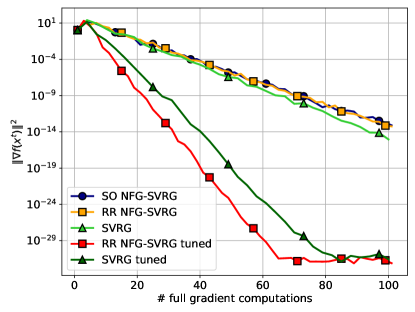
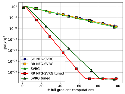
Figure 3: No Full Grad SVRG and SVRG convergence with theoretical and tuned step sizes on problem (8) on the ijcnn1 (left) and a9a (right) datasets.

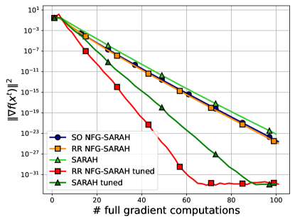
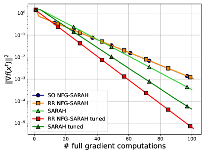
Figure 4: No Full Grad SARAH and SARAH convergence with theoretical and tuned step sizes on problem (8) on the ijcnn1 (left) and a9a (right) datasets.

Upon examining the plots, we notice that although No Full Grad versions may converge slightly slower although comparable than its regular counterpart when using the theoretical step size, it significantly outperforms SVRG and SARAH, respectively, when the step size is optimally tuned. This highlights the potential of our method to achieve superior convergence rates with proper parameter adjustments, providing a robust alternative for large-scale optimization.

A.2 ResNet-18 on CIFAR-10/CIFAR-100 classification.

Optimizers and Experimental Design.

The experiments were implemented in Python using the PyTorch library [Paszke et al., 2019], leveraging both a single CPU (Intel Xeon 2.20 GHz) and a single GPU (NVIDIA Tesla P100) for computation. To emulate a distributed environment, we split batches across multiple workers, simulating a decentralized optimization setting.

Our algorithms are evaluated in terms of accuracy and the number of full gradient computations. The experiments are conducted with the following setup:

• number of workers $M=5$;

• learning rate $\gamma=0.01$ for both optimizers;

• regularization parameters $\lambda_{1}=\lambda_{2}=0.0005$.

The experiments on CIFAR-100 are presented below.

The SVRG algorithm follows a similar trend, with test loss stabilizing instead of increasing, unlike SGD. While SGD rebounds, SVRG maintains a plateau before further improvement. Test accuracy surpasses SGD from epoch 50 onward.

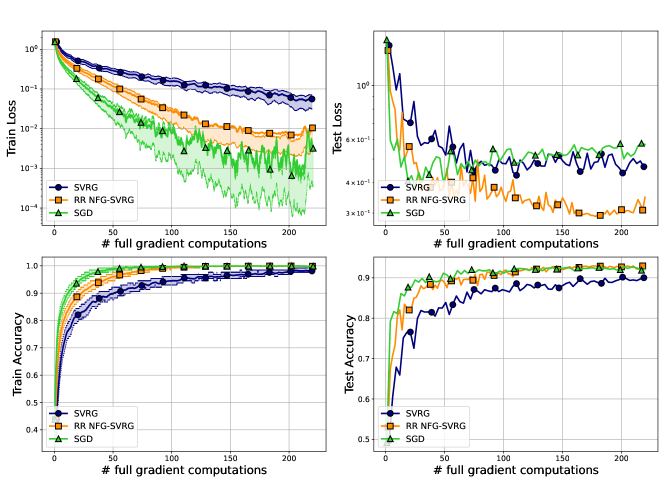
Figure 5: No Full Grad SVRG and SVRG on CIFAR-100 convergence.

The SARAH algorithm stabilizes training loss convergence and outpaces standard SARAH. Test loss decreases beyond SGD’s minimum, leading to a lower final loss. Test accuracy initially rises slowly but later accelerates, reducing overfitting.

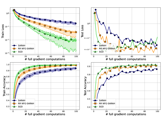
Figure 6: No Full Grad SARAH and SARAH on CIFAR-100 convergence.

Appendix B General Inequalities

We introduce important inequalities that are used in further proofs. Let $f$ adhere to Assumption 1, $g$ adhere to Assumption 2(a). Then for any real number $i$ and for all vectors $x,y,\{x_{i}\}\in\mathbb{R}^{d}$ with a positive scalars $\alpha,\beta$, the following inequalities hold:

$$2\langle x,y\rangle \leqslant\frac{\|x\|^{2}}{\alpha}+\alpha\|y\|^{2},$$ (Scalar)

$$2\langle x,y\rangle =\|x+y\|^{2}-\|x\|^{2}-\|y\|^{,}$$ (Norm)

$$\|x+y\|^{2} \leqslant(1+\beta)\|x\|^{2}+(1+\frac{1}{\beta})\|y\|^{2},$$ (Quad)

$$f(x) \leqslant f(y)+\langle\nabla f(y),x-y\rangle+\frac{L}{2}\|x-y\|^{2},$$ (Lip)

$$\left\|\sum_{i=1}^{n}x_{i}\right\|^{2} \leqslant n\sum_{i=1}^{n}\|x_{i}\|^{2}\quad\quad(\text{Cauchy-Schwarz}),$$ (CS)

$$g(x)-\inf g \leqslant\frac{1}{2\mu}\|\nabla g(x)\|^{2}\quad\quad(\text{Polyak-Lojasiewicz}).$$ (PL)

Here, (Lip) was derived in [Nesterov et al., 2018] in Theorem 2.1.5.

Appendix C No Full Grad SVRG

For the convenience of the reader, we provide here the short description of Algorithm 1. If we consider it in epoch $s\neq 0$, one can note that the update rule is nothing but

$$\begin{split}\begin{cases}&\text{initial initialization:}\\ &\quad\omega_{s}=x_{s}^{0}=x_{s-1}^{n}\\ &\quad v_{s}=\frac{1}{n}\sum\limits_{t=0}^{n-1}\nabla f_{\pi_{s-1}^{t}}(x_{s-1}^{t})\\ &\text{for all iterations during the epoch}:\\ &\quad v_{s}^{t}=\nabla f_{\pi_{s}^{t}}(x_{s}^{t})-\nabla f_{\pi_{s}^{t}}(\omega_{s})+v_{s}\\ &\quad x_{s}^{t+1}=x_{s}^{t}-\gamma v_{s}^{t}\end{cases}\end{split}$$ (9)

C.1 Non-convex setting

Lemma 5.

Suppose that Assumptions 1, 2 hold. Let the stepsize $\gamma\leqslant\frac{1}{Ln}$. Then for Algorithm 1 it holds

$$f(\omega_{s+1})\leqslant f(\omega_{s})-\frac{\gamma n}{2}\|\nabla f(\omega_{s})\|^{2}+\frac{\gamma n}{2}\left\|\nabla f(\omega_{s})-\frac{1}{n}\sum\limits_{t=0}^{n-1}v_{s}^{t}\right\|^{2}.$$

Proof.

Using the iteration of Algorithm 1 (9), we have

$$f(\omega_{s+1}) ~=f(\omega_{s}-(\omega_{s}-\omega_{s+1}))$$

$$\overset{\eqref{ineq4}}{\leqslant}f(\omega_{s})+\langle\nabla f(\omega_{s}),\omega_{s+1}-\omega_{s}\rangle+\frac{L}{2}\|\omega_{s+1}-\omega_{s}\|^{2}$$

$$~=f(\omega_{s})-\gamma n\left\langle\nabla f(\omega_{s}),\frac{1}{n}\sum\limits_{t=0}^{n-1}v_{s}^{t}\right\rangle+\frac{\gamma^{2}n^{2}L}{2}\left\|\frac{1}{n}\sum\limits_{t=0}^{n-1}v_{s}^{t}\right\|^{2}$$

$$~\overset{\eqref{ineq:norm}}{=}f(\omega_{s})-\frac{\gamma n}{2}\left[\|\nabla f(\omega_{s})\|^{2}+\left\|\frac{1}{n}\sum\limits_{t=0}^{n-1}v_{s}^{t}\right\|^{2}-\left\|\nabla f(\omega_{s})-\frac{1}{n}\sum\limits_{t=0}^{n-1}v_{s}^{t}\right\|^{2}\right]$$

$$\quad~+\frac{\gamma^{2}n^{2}L}{2}\left\|\frac{1}{n}\sum\limits_{t=0}^{n-1}v_{s}^{t}\right\|^{2}$$

$$~=f(\omega_{s})-\frac{\gamma n}{2}\left[\|\nabla f(\omega_{s})\|^{2}-\left\|\nabla f(\omega_{s})-\frac{1}{n}\sum\limits_{t=0}^{n-1}v_{s}^{t}\right\|^{2}\right]$$

$$\quad~-\frac{\gamma n}{2}\cdot\left(1-\gamma nL\right)\left\|\frac{1}{n}\sum\limits_{t=0}^{n-1}v_{s}^{t}\right\|^{2},$$

Choosing $\gamma:\frac{\gamma n}{2}\left(1-\gamma nL\right)>0$ and note that such a choice is followed by $\gamma\leqslant\frac{1}{Ln}$. In that way, we make the last term is negative and obtain the result of the lemma. ∎

Now we want to address the last term in the inequality of Lemma 5. We prove the following lemma.

Lemma 6 (Lemma 1).

Suppose that Assumptions 1, 2 hold. Then for Algorithm 1 a valid estimate is

$$\left\|\nabla f(\omega_{s})-\frac{1}{n}\sum\limits_{t=0}^{n-1}v_{s}^{t}\right\|^{2} \leqslant 2\|\nabla f(\omega_{s})-v_{s}\|^{2}+\frac{2L^{2}}{n}\sum\limits_{t=0}^{n-1}\|x_{s}^{t}-\omega_{s}\|^{2}.$$

Proof.

We straightforwardly move to estimate of the desired norm:

$$\left\|\nabla f(\omega_{s})-\frac{1}{n}\sum\limits_{t=0}^{n-1}v_{s}^{t}\right\|^{2} \overset{\eqref{svrg:update}}{=}\left\|\nabla f(\omega_{s})-\frac{1}{n}\left(nv_{s}+\sum\limits_{t=0}^{n-1}\left(\nabla f_{\pi_{s}^{t}}(x_{s}^{t})-\nabla f_{\pi_{s}^{t}}(\omega_{s})\right)\right)\right\|^{2}$$

$$\overset{\eqref{ineq1}}{\leqslant}2\|\nabla f(\omega_{s})-v_{s}\|^{2}+\frac{2}{n^{2}}\left\|\sum\limits_{t=0}^{n-1}\left(\nabla f_{\pi_{s}^{t}}(x_{s}^{t})-\nabla f_{\pi_{s}^{t}}(\omega_{s})\right)\right\|^{2}$$

$$\overset{\eqref{ineq1}}{\leqslant}2\|\nabla f(\omega_{s})-v_{s}\|^{2}+\frac{2}{n}\sum\limits_{t=0}^{n-1}\left\|\nabla f_{\pi_{s}^{t}}(x_{s}^{t})-\nabla f_{\pi_{s}^{t}}(\omega_{s})\right\|^{2}$$

$$\overset{\text{Ass. \ref{as1}}}{\leqslant}2\|\nabla f(\omega_{s})-v_{s}\|^{2}+\frac{2L^{2}}{n}\sum\limits_{t=0}^{n-1}\left\|x_{s}^{t}-\omega_{s}\right\|^{2},$$ (10)

which ends the proof. ∎

Lemma 7 (Lemma 2).

Suppose that Assumptions 1, 2 hold. Let the stepsize $\gamma\leqslant\frac{1}{2Ln}$. Then for Algorithm 1 a valid estimate is

$$\left\|\nabla f(\omega_{s})-\frac{1}{n}\sum\limits_{t=0}^{n-1}v_{s}^{t}\right\|^{2} \leqslant 8\gamma^{2}L^{2}n^{2}\|v_{s}\|^{2}+32\gamma^{2}L^{2}n^{2}\|v_{s-1}\|^{2}.$$

Proof.

To begin with, in Lemma 6, we obtain

$$\left\|\nabla f(\omega_{s})-\frac{1}{n}\sum\limits_{t=0}^{n-1}v_{s}^{t}\right\|^{2}\leqslant 2\|\nabla f(\omega_{s})-v_{s}\|^{2}+\frac{2L^{2}}{n}\sum\limits_{t=0}^{n-1}\|x_{s}^{t}-\omega_{s}\|^{2}.$$ (11)

Let us show what $v_{s}$ is (here we use Line 7 of Algorithm 1):

$$v_{s} =\widetilde{v}_{s-1}^{n}=\frac{n-1}{n}\widetilde{v}_{s-1}^{n-1}+\frac{1}{n}\nabla f_{\pi_{s-1}^{n-1}}(x_{s-1}^{n-1})$$

$$=\frac{n-1}{n}\cdot\frac{n-2}{n-1}\widetilde{v}_{s-1}^{n-2}+\frac{n-1}{n}\cdot\frac{1}{n-1}\nabla f_{\pi_{s-1}^{n-2}}(x_{s-1}^{n-2})+\frac{1}{n}\nabla f_{\pi_{s-1}^{n-1}}(x_{s-1}^{n-1})$$

$$=\frac{n-1}{n}\cdot\frac{n-2}{n-1}\cdot\ldots\cdot 0\cdot\widetilde{v}_{s-1}^{0}+\frac{1}{n}\sum\limits_{t=0}^{n-1}\nabla f_{\pi_{s-1}^{t}}(x_{s-1}^{t})$$

$$\overset{(i)}{=}\frac{1}{n}\sum\limits_{t=0}^{n-1}\nabla f_{\pi_{s-1}^{t}}(x_{s-1}^{t}),$$ (12)

where equation (i) is correct due to initialization $\widetilde{v}_{s-1}^{0}=0$ (Line 13 of Algorithm 1). In that way, using (11) and (12),

$$\left\|\nabla f(\omega_{s})-\frac{1}{n}\sum\limits_{t=0}^{n-1}v_{s}^{t}\right\|^{2} \leqslant 2\left\|\nabla f(\omega_{s})-\frac{1}{n}\sum\limits_{t=0}^{n-1}\nabla f_{\pi_{s-1}^{t}}(x_{s-1}^{t})\right\|^{2}$$

$$~~+\frac{2L^{2}}{n}\sum\limits_{t=0}^{n-1}\|x_{s}^{t}-\omega_{s}\|^{2}.$$

Then, using (1),

$$\left\|\nabla f(\omega_{s})-\frac{1}{n}\sum\limits_{t=0}^{n-1}v_{s}^{t}\right\|^{2} \leqslant~~2\left\|\frac{1}{n}\sum\limits_{t=0}^{n-1}\left(\nabla f_{\pi_{s-1}^{t}}(\omega_{s})-\nabla f_{\pi_{s-1}^{t}}(x_{s-1}^{t})\right)\right\|^{2}+\frac{2L^{2}}{n}\sum\limits_{t=0}^{n-1}\|x_{s}^{t}-\omega_{s}\|^{2}$$

$$\overset{\eqref{ineq1}}{\leqslant}\frac{2}{n}\sum\limits_{t=0}^{n-1}\|\nabla f_{\pi_{s-1}^{t}}(\omega_{s})-\nabla f_{\pi_{s-1}^{t}}(x_{s-1}^{t})\|^{2}+\frac{2L^{2}}{n}\sum\limits_{t=0}^{n-1}\|x_{s}^{t}-\omega_{s}\|^{2}$$

$$\overset{\text{Ass. \ref{as1}}}{\leqslant}\frac{2L^{2}}{n}\sum\limits_{t=0}^{n-1}\|x_{s-1}^{t}-\omega_{s}\|^{2}+\frac{2L^{2}}{n}\sum\limits_{t=0}^{n-1}\|x_{s}^{t}-\omega_{s}\|^{2}$$

$$\overset{\eqref{ineq:square}}{\leqslant}\frac{4L^{2}}{n}\sum\limits_{0}^{n-1}\|x_{s-1}^{t}-\omega_{s-1}\|^{2}+\frac{4L^{2}}{n}\sum\limits_{t=0}^{n-1}\|\omega_{s}-\omega_{s-1}\|^{2}$$

$$~~+\frac{2L^{2}}{n}\sum\limits_{t=0}^{n-1}\|x_{s}^{t}-\omega_{s}\|^{2}.$$ (13)

Now we have to bound these three terms. Let us begin with $\sum\limits_{t=0}^{n-1}\|x_{s}^{t}-\omega_{s}\|^{2}$.

$$\sum\limits_{t=0}^{n-1}\|x_{s}^{t}-\omega_{s}\|^{2} =\gamma^{2}\sum\limits_{t=0}^{n-1}\left\|\sum\limits_{k=0}^{t-1}v_{s}^{k}\right\|^{2}\overset{\eqref{svrg:update}}{=}\gamma^{2}\sum\limits_{t=0}^{n-1}\left\|tv_{s}+\sum\limits_{k=0}^{t-1}\left(\nabla f_{\pi_{s}^{k}}(x_{s}^{k})-\nabla f_{\pi_{s}^{k}}(\omega_{s})\right)\right\|^{2}$$

$$\overset{\eqref{ineq1}}{\leqslant}2\gamma^{2}\sum\limits_{t=0}^{n-1}t^{2}\|v_{s}\|^{2}+2\gamma^{2}\sum\limits_{t=0}^{n-1}t\sum\limits_{k=0}^{t-1}\|\nabla f_{\pi_{s}^{k}}(x_{s}^{k})-\nabla f_{\pi_{s}^{k}}(\omega_{s})\|^{2}$$

$$\overset{\text{Ass. \ref{as1}}}{\leqslant}2\gamma^{2}n^{3}\|v_{s}\|^{2}+2\gamma^{2}L^{2}n\sum\limits_{t=0}^{n-1}\sum\limits_{k=0}^{t-1}\|x_{s}^{k}-\omega_{s}\|^{2}$$

$$~~\leqslant~~2\gamma^{2}n^{3}\|v_{s}\|^{2}+2\gamma^{2}L^{2}n^{2}\sum\limits_{t=0}^{n-2}\|x_{s}^{t}-\omega_{s}\|^{2}$$

$$~~\leqslant~~2\gamma^{2}n^{3}\|v_{s}\|^{2}+2\gamma^{2}L^{2}n^{2}\sum\limits_{t=0}^{n-1}\|x_{s}^{t}-\omega_{s}\|^{2}.$$

Expressing $\sum\limits_{t=0}^{n-1}\|x_{s}^{t}-\omega_{s}\|^{2}$ from here, we get

$$\sum\limits_{t=0}^{n-1}\|x_{s}^{t}-\omega_{s}\|^{2}\leqslant\frac{2\gamma^{2}n^{3}\|v_{s}\|^{2}}{1-2\gamma^{2}L^{2}n^{2}}.$$

To finish this part of proof it remains for us to choose appropriate $\gamma$. In Lemma 5 we require $\gamma\leqslant\frac{1}{Ln}$. There we choose smaller values of $\gamma:\gamma\leqslant\frac{1}{2Ln}$ (with that values all previous transitions is correct). Now we provide final estimation of this norm:

$$\sum\limits_{t=0}^{n-1}\|x_{s}^{t}-\omega_{s}\|^{2}\leqslant 4\gamma^{2}n^{3}\|v_{s}\|^{2}.$$ (14)

One can note the boundary of the $\sum\limits_{t=0}^{n-1}\|x_{s-1}^{t}-\omega_{s-1}\|^{2}$ term is similar because it involves the same sum of norms from the previous epoch.

$$\sum\limits_{t=0}^{n}\|x_{s-1}^{t}-\omega_{s-1}\|^{2}\leqslant 4\gamma^{2}n^{3}\|v_{s-1}\|^{2}.$$ (15)

It remains for us to estimate the $\sum\limits_{t=0}^{n-1}\|\omega_{s}-\omega_{s-1}\|^{2}$ term.

$$\sum\limits_{t=0}^{n-1}\|\omega_{s}-\omega_{s-1}\|^{2} ~~=~~\gamma^{2}\sum\limits_{t=0}^{n-1}\left\|\sum\limits_{k=0}^{n-1}v_{s-1}^{k}\right\|^{2}$$

$$~~\overset{\eqref{svrg:update}}{=}~~\gamma^{2}\sum\limits_{t=0}^{n-1}\left\|nv_{s-1}+\sum\limits_{k=0}^{n-1}\left(\nabla f_{\pi_{s-1}^{k}}(x_{s-1}^{k})-\nabla f_{\pi_{s-1}^{k}}(\omega_{s-1})\right)\right\|^{2}$$

$$~~\overset{\eqref{ineq1}}{\leqslant}~~2\gamma^{2}\sum\limits_{t=0}^{n-1}n^{2}\|v_{s-1}\|^{2}+2\gamma^{2}\sum\limits_{t=0}^{n-1}n\sum\limits_{k=0}^{n-1}\|\nabla f_{\pi_{s-1}^{k}}(x_{s-1}^{k})-\nabla f_{\pi_{s-1}^{k}}(\omega_{s-1})\|^{2}$$

$$\overset{\text{Ass. \ref{as1}}}{\leqslant}~~2\gamma^{2}n^{3}\|v_{s-1}\|^{2}+2\gamma^{2}L^{2}n\sum\limits_{t=0}^{n-1}\sum\limits_{k=0}^{t-1}\|x_{s-1}^{k}-\omega_{s-1}\|^{2}$$

$$\quad\leqslant~~2\gamma^{2}n^{3}\|v_{s-1}\|^{2}+2\gamma^{2}L^{2}n^{2}\sum\limits_{t=0}^{n-2}\|x_{s-1}^{t}-\omega_{s-1}\|^{2}$$

$$\quad\leqslant~~2\gamma^{2}n^{3}\|v_{s-1}\|^{2}+2\gamma^{2}L^{2}n^{2}\sum\limits_{t=0}^{n-1}\|x_{s-1}^{t}-\omega_{s-1}\|^{2}$$

$$\quad\overset{\eqref{l3:ineq5}}{\leqslant}~~2\gamma^{2}n^{3}\|v_{s-1}\|^{2}+8\gamma^{4}L^{2}n^{5}\sum\limits_{t=0}^{n-1}\|x_{s-1}^{t}-\omega_{s-1}\|^{2}.$$

Using our choice $\gamma\leqslant\frac{1}{2Ln}$, we derive the estimate of the last term:

$$\sum\limits_{t=0}^{n-1}\|\omega_{s}-\omega_{s-1}\|^{2}\leqslant 2\gamma^{2}n^{3}\|v_{s-1}\|^{2}+2\gamma^{2}n^{3}\|v_{s-1}\|^{2}=4\gamma^{2}n^{3}\|v_{s-1}\|^{2}.$$ (16)

Now we can apply the upper bounds obtained in (14) – (16) to (13) and have

$$\left\|\nabla f(\omega_{s})-\frac{1}{n}\sum\limits_{t=0}^{n-1}v_{s}^{t}\right\|^{2} \leqslant 8\gamma^{2}L^{2}n^{2}\|v_{s}\|^{2}+16\gamma^{2}L^{2}n^{2}\|v_{s-1}\|^{2}+16\gamma^{2}L^{2}n^{2}\|v_{s-1}\|^{2}$$

$$=8\gamma^{2}L^{2}n^{2}\|v_{s}\|^{2}+32\gamma^{2}L^{2}n^{2}\|v_{s-1}\|^{2},$$

which ends the proof. ∎

Theorem 7 (Theorem 1).

Suppose Assumptions 1, 2(b) hold. Then Algorithm 1 with $\gamma\leqslant\frac{1}{20Ln}$ to reach $\varepsilon$-accuracy, where $\varepsilon^{2}=\frac{1}{S}\sum\limits_{s=1}^{S}\|\nabla f(\omega_{s})\|^{2}$, needs

$$\mathcal{O}\left(\frac{nL}{\varepsilon^{2}}\right)~~\text{iterations and oracle calls.}$$

Proof.

We combine the result of Lemma 5 with the result of Lemma 7 and obtain

$$f(\omega_{s+1}) \leqslant f(\omega_{s})-\frac{\gamma n}{2}\|\nabla f(\omega_{s})\|^{2}$$

$$\quad+\frac{\gamma n}{2}\left(8\gamma^{2}L^{2}n^{2}\|v_{s}\|^{2}+32\gamma^{2}L^{2}n^{2}\|v_{s-1}\|^{2}\right).$$

We subtract $f(x^{*})$ from both parts:

$$f(\omega_{s+1})-f(x^{*}) \leqslant f(\omega_{s})-f(x^{*})-\frac{\gamma n}{2}\|\nabla f(\omega_{s})\|^{2}$$

$$\quad+\frac{\gamma n}{2}\left(8\gamma^{2}L^{2}n^{2}\|v_{s}\|^{2}+32\gamma^{2}L^{2}n^{2}\|v_{s-1}\|^{2}\right)$$

$$=f(\omega_{s})-f(x^{*})-\frac{\gamma n}{4}\|\nabla f(\omega_{s})\|^{2}$$

$$\quad+\frac{\gamma n}{2}\left(8\gamma^{2}L^{2}n^{2}\|v_{s}\|^{2}+32\gamma^{2}L^{2}n^{2}\|v_{s-1}\|^{2}\right)$$

$$\quad-\frac{\gamma n}{4}\|\nabla f(\omega_{s})\|^{2}.$$

Then, transforming the last term by using (Quad) with $\beta=1$, we get

$$f(\omega_{s+1})-f(x^{*}) \leqslant f(\omega_{s})-f(x^{*})-\frac{\gamma n}{4}\|\nabla f(\omega_{s})\|^{2}$$

$$\quad+\frac{\gamma n}{2}\left(8\gamma^{2}L^{2}n^{2}\|v_{s}\|^{2}+32\gamma^{2}L^{2}n^{2}\|v_{s-1}\|^{2}\right)$$

$$\quad-\frac{\gamma n}{8}\|v_{s}\|^{2}+\frac{\gamma n}{4}\|v_{s}-\nabla f(x\omega_{s})\|^{2}.$$

Using Lemma 7 to $\|v_{s}-\nabla f(\omega_{s})\|^{2}$ (specially $\frac{4L^{2}}{n}\cdot\eqref{l3:ineq5}+\frac{4L^{2}}{n}\cdot\eqref{l3:ineq6}$),

$$f(\omega_{s+1})-f(x^{*}) \leqslant f(\omega_{s})-f(x^{*})-\frac{\gamma n}{4}\|\nabla f(\omega_{s})\|^{2}$$

$$\quad+\frac{\gamma n}{2}\left(8\gamma^{2}L^{2}n^{2}\|v_{s}\|^{2}+32\gamma^{2}L^{2}n^{2}\|v_{s-1}\|^{2}\right)$$

$$\quad-\frac{\gamma n}{8}\|v_{s}\|^{2}+\frac{\gamma n}{4}\cdot 32\gamma^{2}L^{2}n^{2}\|v_{s-1}\|^{2}.$$

Combining alike expressions,

$$f(\omega_{s+1})-f(x^{*})+\frac{\gamma n}{4}\|\nabla f(\omega_{s})\|^{2} \leqslant f(\omega_{s})-f(x^{*})-\frac{\gamma n}{8}\left(1-32\gamma^{2}L^{2}n^{2}\right)\|v_{s}\|^{2}$$

$$\quad+\gamma n\cdot 24\gamma^{2}L^{2}n^{2}\|v_{s-1}\|^{2}.$$ (17)

Using $\gamma\leqslant\frac{1}{20Ln}$ (note it is the smallest stepsize from all the steps we used before, so all previous transitions are correct), we get

$$f(\omega_{s+1})-f(x^{*}) +\frac{1}{10}\gamma n\|v_{s}\|^{2}+\frac{\gamma(n+1)}{4}\|\nabla f(\omega_{s})\|^{2}$$

$$\leqslant f(\omega_{s})-f(x^{*})+\frac{1}{10}\gamma n\|v_{s-1}\|^{2}.$$

Next, denoting $\Delta_{s}=f(\omega_{s+1})-f(x^{*})+\frac{1}{10}\gamma n\|v_{s}\|^{2}$, we obtain

$$\frac{1}{S}\sum\limits_{s=1}^{S}\|\nabla f(\omega_{s})\|^{2}\leqslant\frac{4\left[\Delta_{0}-\Delta_{S}\right]}{\gamma nS}.$$

We choose $\varepsilon^{2}=\frac{1}{S}\sum\limits_{s=1}^{S}\|\nabla f(\omega_{s})\|^{2}$ as criteria. Hence, to reach $\varepsilon$-accuracy we need $\mathcal{O}\left(\frac{L}{\varepsilon^{2}}\right)$ epochs and $\mathcal{O}\left(\frac{nL}{\varepsilon^{2}}\right)$ iterations. Additionally, we note that the oracle complexity of our algorithm is also equal to $\mathcal{O}(\frac{nL}{\varepsilon^{2}})$, since at each iteration the algorithm computes the stochastic gradient at only two points. This ends the proof. ∎

C.2 Strongly convex setting

Theorem 8 (Theorem 2).

Suppose Assumptions 1, 2(a) hold. Then Algorithm 1 with $\gamma\leqslant\frac{1}{20Ln}$ to reach $\varepsilon$-accuracy, where $\varepsilon=f(x_{S+1}^{0})-f(x^{*})$, needs

$$\mathcal{O}\left(\frac{nL}{\mu}\log\frac{1}{\varepsilon}\right)~~\text{iterations and oracle calls.}$$

Proof.

Under Assumption 2(a), which states that the function is strongly convex, the (PL) condition is automatically satisfied. Therefore,

$$f(\omega_{s+1})-f(x^{*})+\frac{\gamma\mu n}{2}\left(f(\omega_{s})-f(x^{*})\right) \leqslant f(\omega_{s+1})-f(x^{*})+\frac{\gamma n}{4}\|\nabla f(\omega_{s})\|^{2}.$$

Thus, using (17),

$$f(\omega_{s+1})-f(x^{*}) +\frac{\gamma\mu n}{2}\left(f(\omega_{s})-f(x^{*})\right)\leqslant f(\omega_{s})-f(x^{*})$$

$$-\frac{\gamma n}{8}\left(1-32\gamma^{2}L^{2}n^{2}\right)\|v_{s}\|^{2}+\gamma n\cdot 24\gamma^{2}L^{2}n^{2}\|v_{s-1}\|^{2}.$$

Using $\gamma\leqslant\frac{1}{20L(n+1)}$ and assuming $n\geqslant 2$, we get

$$f(\omega_{s+1})-f(x^{*})+\frac{1}{10}\gamma n\|v_{s}\|^{2} \leqslant\left(1-\frac{\gamma\mu n}{2}\right)\left(f(\omega_{s})-f(x^{*})\right)$$

$$\quad+\frac{1}{10}\gamma n\cdot\left(1-\frac{\gamma\mu n}{2}\right)\|v_{s-1}\|^{2}.$$

Next, denoting $\Delta_{s}=f(\omega_{s+1})-f(x^{*})+\frac{1}{10}\gamma n\|v_{s}\|^{2}$, we obtain the final convergence over one epoch:

$$\Delta_{s+1}\leqslant\left(1-\frac{\gamma\mu n}{2}\right)\Delta_{s}.$$

Going into recursion over all epoch,

$$f(\omega_{S+1})-f(x^{*})\leqslant\Delta_{S}\leqslant\left(1-\frac{\gamma\mu n}{2}\right)^{S+1}\Delta_{0}.$$

We choose $\varepsilon=f(\omega_{S+1})-f(x^{*})$ as criteria. Then to reach $\varepsilon$-accuracy we need $\mathcal{O}\left(\frac{L}{\mu}\log\left(\frac{1}{\varepsilon}\right)\right)$ epochs and $\mathcal{O}\left(\frac{nL}{\mu}\log\left(\frac{1}{\varepsilon}\right)\right)$ iterations. Additionally, we note that the oracle complexity of our algorithm is also equal to $\mathcal{O}\left(\frac{nL}{\mu}\log\left(\frac{1}{\varepsilon}\right)\right)$, since at each iteration the algorithm computes the stochastic gradient at only two points. ∎

Appendix D No Full Grad SARAH

For the convenience of the reader, we provide here the short description of Algorithm 2. If we consider it in epoch $s\neq 0$, one can note that the update rule is nothing but

$$\begin{split}\begin{cases}&\text{if iteration~}t=0:\\ &\quad x_{s}^{0}=x_{s-1}^{n}\\ &\quad v_{s}^{0}=v_{s}=\frac{1}{n}\sum\limits_{t=1}^{n}\nabla f_{\pi_{s-1}^{t}}(x_{s-1}^{t})\\ &\quad x_{s}^{1}=x_{s}^{0}-\gamma v_{s}^{0}\\ &\text{for rest iterations during the epoch}:\\ &\quad v_{s}^{t}=v_{s}^{t-1}+\frac{1}{n}\left(\nabla f_{\pi_{s}^{t}}(x_{s}^{t})-\nabla f_{\pi_{s}^{t}}(\omega_{s})\right)\\ &\quad x_{s}^{t+1}=x_{s}^{t}-\gamma v_{s}^{t}\end{cases}\end{split}$$ (18)

D.1 Non-convex setting

Lemma 8.

Suppose that Assumptions 1, 2 hold. Let the stepsize $\gamma\leqslant\frac{1}{L(n+1)}$. Then for Algorithm 2 it holds

$$f(x_{s+1}^{0})\leqslant f(x_{s}^{0})-\frac{\gamma(n+1)}{2}\|\nabla f(x_{s}^{0})\|^{2}+\frac{\gamma(n+1)}{2}\left\|\nabla f(x_{s}^{0})-\frac{1}{n+1}\sum\limits_{i=0}^{n}v_{s}^{i}\right\|^{2}.$$

Proof.

Using the iteration of Algorithm 2 (18), we have

$$f(x_{s+1}^{0}) ~=f(x_{s}^{0}-(x_{s}^{0}-x_{s+1}^{0}))$$

$$\overset{\eqref{ineq4}}{\leqslant}f(x_{s}^{0})+\langle\nabla f(x_{s}^{0}),x_{s+1}^{0}-x_{s}^{0}\rangle+\frac{L}{2}\|x_{s+1}^{0}-x_{s}^{0}|^{2}$$

$$~=f(x_{s}^{0})-\gamma(n+1)\left\langle\nabla f(x_{s}^{0}),\frac{1}{n+1}\sum\limits_{t=0}^{n}v_{s}^{t}\right\rangle+\frac{\gamma^{2}(n+1)^{2}L}{2}\left\|\frac{1}{n+1}\sum\limits_{t=0}^{n}v_{s}^{t}\right\|^{2}$$

$$~\overset{\eqref{ineq:norm}}{=}f(x_{s}^{0})-\frac{\gamma(n+1)}{2}\left[\|\nabla f(x_{s}^{0})\|^{2}+\left\|\frac{1}{n+1}\sum\limits_{t=0}^{n}v_{s}^{t}\right\|^{2}-\left\|\nabla f(x_{s}^{0})-\frac{1}{n+1}\sum\limits_{t=0}^{n}v_{s}^{t}\right\|^{2}\right]$$

$$\quad~+\frac{\gamma^{2}(n+1)^{2}L}{2}\left\|\frac{1}{n+1}\sum\limits_{t=0}^{n}v_{s}^{t}\right\|^{2}$$

$$~=f(x_{s}^{0})-\frac{\gamma(n+1)}{2}\left[\|\nabla f(x_{s}^{0})\|^{2}-\left\|\nabla f(x_{s}^{0})-\frac{1}{n+1}\sum\limits_{t=0}^{n}v_{s}^{t}\right\|^{2}\right]$$

$$\quad~-\frac{\gamma(n+1)}{2}\cdot\left(1-\gamma(n+1)L\right)\left\|\frac{1}{n+1}\sum\limits_{t=0}^{n}v_{s}^{t}\right\|^{2}.$$

It remains for us to choose $\gamma:\frac{\gamma(n+1)}{2}\left(1-\gamma(n+1)L\right)>0$ and note that such a choice is followed by $\gamma\leqslant\frac{1}{L(n+1)}$. In that way we make the last term is negative and obtain the result of the lemma. ∎

Now we want to address the last term in the result of Lemma 8. We prove the following lemma.

Lemma 9 (Lemma 3).

Suppose that Assumptions 1, 2 hold. Then for Algorithm 2 a valid estimate is

$$\left\|\nabla f(x_{s}^{0})-\frac{1}{n+1}\sum\limits_{t=0}^{n}v_{s}^{t}\right\|^{2} \leqslant 2\|\nabla f(x_{s}^{0})-v_{s}\|^{2}+\frac{2L^{2}}{n+1}\sum\limits_{t=1}^{n}\|x_{s}^{t}-x_{s}^{t-1}\|^{2}.$$

Proof.

We claim that

$$\sum\limits_{t=k}^{n}v_{s}^{t}=\frac{1}{n}\sum\limits_{t=k+1}^{n}(n-t+1)\left(\nabla f_{\pi_{s}^{t}}(x_{s}^{t})-\nabla f_{\pi_{s}^{t}}(x_{s}^{t-1})\right)+(n-k+1)v_{s}^{k}.$$ (19)

Let us prove this. We use the method of induction. For $k=n$ it is obviously true. We suppose that it is true for some some fixed $k=\widetilde{k}\geqslant 1$ ($k=0$ is the first index in the epoch, i.e. start of the recursion) and want to prove that it is true for $k=\widetilde{k}-1$.

$$\sum\limits_{t=\widetilde{k}-1}^{n}v_{s}^{t} =v_{s}^{\widetilde{k}-1}+\sum\limits_{t=\widetilde{k}}^{n}v_{s}^{t}$$

$$=v_{s}^{\widetilde{k}-1}+\frac{1}{n}\sum\limits_{t=\widetilde{k}+1}^{n}(n-t+1)\left(\nabla f_{\pi_{s}^{t}}(x_{s}^{t})-\nabla f_{\pi_{s}^{t}}(x_{s}^{t-1})\right)+(n-\widetilde{k}+1)v_{s}^{\widetilde{k}}$$

$$\overset{(i)}{=}v_{s}^{\widetilde{k}-1}+\frac{1}{n}\sum\limits_{t=\widetilde{k}+1}^{n}(n-t+1)\left(\nabla f_{\pi_{s}^{t}}(x_{s}^{t})-\nabla f_{\pi_{s}^{t}}(x_{s}^{t-1})\right)$$

$$\quad+(n-\widetilde{k}+1)\left(v_{s}^{\widetilde{k}-1}+\frac{1}{n}\left(\nabla f_{\pi_{s}^{\widetilde{k}}}(x_{s}^{\widetilde{k}})-\nabla f_{\pi_{s}^{\widetilde{k}}}(x_{s}^{\widetilde{k}-1})\right)\right)$$

$$=\frac{1}{n}\sum\limits_{t=\widetilde{k}}^{n}(n-t+1)\left(\nabla f_{\pi_{s}^{t}}(x_{s}^{t})-\nabla f_{\pi_{s}^{t}}(x_{s}^{t-1})\right)+(n-\widetilde{k}+2)v_{s}^{\widetilde{k}-1},$$

where equation (i) is correct due to (18) and $\widetilde{k}\geqslant 1$. In that way, the induction step is proven. It means that (19) is valid. We substitute $k=0$ in (19) and, utilizing $v_{s}^{0}=v_{s}$, get

$$\sum\limits_{t=0}^{n}v_{s}^{t} =\frac{1}{n}\sum\limits_{t=1}^{n}(n-t+1)\left(\nabla f_{\pi_{s}^{t}}(x_{s}^{t})-\nabla f_{\pi_{s}^{t}}(x_{s}^{t-1})\right)+(n+1)v_{s}.$$ (20)

Hence, estimating the desired term gives

$$\Biggl{\|}\nabla f(x_{s}^{0})-\frac{1}{n+1}\sum\limits_{t=0}^{n}v_{s}^{t}\Biggr{\|}^{2} ~=\frac{1}{(n+1)^{2}}\left\|(n+1)\nabla f(x_{s}^{0})-\sum\limits_{t=0}^{n}v_{s}^{t}\right\|^{2}$$

$$~\overset{\eqref{l5:ineq2}}{=}\frac{1}{(n+1)^{2}}\Biggl{\|}(n+1)\nabla f(x_{s}^{0})$$

$$\quad-\frac{1}{n}\sum\limits_{t=1}^{n}(n-t+1)\left(\nabla f_{\pi_{s}^{t}}(x_{s}^{t})-\nabla f_{\pi_{s}^{t}}(x_{s}^{t-1})\right)-(n+1)v_{s}\Biggr{\|}^{2}$$

$$~~\overset{\eqref{ineq1}}{\leqslant}2\|\nabla f(x_{s}^{0})-v_{s}\|^{2}$$

$$\quad+\frac{2}{(n+1)^{2}}\left\|\frac{1}{n}\sum\limits_{t=1}^{n}(n-t+1)\left(\nabla f_{\pi_{s}^{t}}(x_{s}^{t})-\nabla f_{\pi_{s}^{t}}(x_{s}^{t-1})\right)\right\|^{2}$$

$$~~\overset{(i)}{\leqslant}2\|\nabla f(x_{s}^{0})-v_{s}\|^{2}+\frac{2}{(n+1)^{2}}\left\|\sum\limits_{t=1}^{n}\left(\nabla f_{\pi_{s}^{t}}(x_{s}^{t})-\nabla f_{\pi_{s}^{t}}(x_{s}^{t-1})\right)\right\|^{2}$$

$$~~\overset{\eqref{ineq1}}{\leqslant}2\|\nabla f(x_{s}^{0})-v_{s}\|^{2}+\frac{2}{n+1}\sum\limits_{t=1}^{n}\left\|\nabla f_{\pi_{s}^{t}}(x_{s}^{t})-\nabla f_{\pi_{s}^{t}}(x_{s}^{t-1})\right\|^{2}$$

$$~~\overset{\text{Ass. \ref{as1}}}{\leqslant}2\|\nabla f(x_{s}^{0})-v_{s}\|^{2}+\frac{2L^{2}}{n+1}\sum\limits_{t=1}^{n}\left\|x_{s}^{t}-x_{s}^{t-1}\right\|^{2},$$

where inequality (i) is correct due to $t\geqslant 1$ holds during the summation. The obtained inequality finishes the proof of the lemma. ∎

Lemma 10 (Lemma 4).

Suppose that Assumptions 1, 2 hold. Let the stepsize $\gamma\leqslant\frac{1}{3L}$. Then for Algorithm 2 a valid estimate is

$$\left\|\nabla f(x_{s}^{0})-\frac{1}{n+1}\sum\limits_{t=0}^{n}v_{s}^{t}\right\|^{2} \leqslant 9\gamma^{2}L^{2}\|v_{s}\|^{2}+36\gamma^{2}L^{2}n^{2}\|v_{s-1}\|^{2}.$$

Proof.

To begin with, in Lemma 1, we obtain

$$\left\|\nabla f(x_{s}^{0})-\frac{1}{n+1}\sum\limits_{t=0}^{n}v_{s}^{t}\right\|^{2}\leqslant 2\|\nabla f(x_{s}^{0})-v_{s}\|^{2}+\frac{2L^{2}}{n+1}\sum\limits_{t=1}^{n}\|x_{s}^{t}-x_{s}^{t-1}\|^{2}.$$ (21)

Let us show what $v_{s}$ is (here we use Line 9 of Algorithm 2):

$$v_{s} =\widetilde{v}_{s-1}^{n+1}=\frac{n-1}{n}\widetilde{v}_{s-1}^{n}+\frac{1}{n}\nabla f_{\pi_{s-1}^{n}}(x_{s-1}^{n})$$

$$=\frac{n-1}{n}\cdot\frac{n-2}{n-1}\widetilde{v}_{s-1}^{n-1}+\frac{n-1}{n}\cdot\frac{1}{n-1}\nabla f_{\pi_{s-1}^{n-1}}(x_{s-1}^{n-1})+\frac{1}{n}\nabla f_{\pi_{s-1}^{n}}(x_{s-1}^{n})$$

$$=\frac{n-1}{n}\cdot\frac{n-2}{n-1}\cdot\ldots\cdot 0\cdot\widetilde{v}_{s-1}^{1}+\frac{1}{n}\sum\limits_{t=1}^{n}\nabla f_{\pi_{s-1}^{t}}(x_{s-1}^{t})$$

$$\overset{(i)}{=}\frac{1}{n}\sum\limits_{t=1}^{n}\nabla f_{\pi_{s-1}^{t}}(x_{s-1}^{t}),$$ (22)

where equation (i) is correct due to initialization $\widetilde{v}_{s-1}^{1}=0$ (Line 14 of Algorithm 2). In that way, using (21) and (22),

$$\left\|\nabla f(x_{s}^{0})-\frac{1}{n+1}\sum\limits_{t=0}^{n}v_{s}^{t}\right\|^{2} \leqslant 2\left\|\nabla f(x_{s}^{0})-\frac{1}{n}\sum\limits_{t=1}^{n}\nabla f_{\pi_{s-1}^{t}}(x_{s-1}^{t})\right\|^{2}$$

$$~~+\frac{2L^{2}}{n+1}\sum\limits_{t=1}^{n}\|x_{s}^{t}-x_{s}^{t-1}\|^{2}.$$

Then, using (1),

$$\left\|\nabla f(x_{s}^{0})-\frac{1}{n+1}\sum\limits_{t=0}^{n}v_{s}^{t}\right\|^{2} ~~~~~\leqslant~~2\left\|\frac{1}{n}\sum\limits_{t=1}^{n}\left[\nabla f_{\pi_{s-1}^{t}}(x_{s}^{0})-\nabla f_{\pi_{s-1}^{t}}(x_{s-1}^{t})\right]\right\|^{2}$$

$$\quad\quad+\frac{2L^{2}}{n+1}\sum\limits_{t=1}^{n}\|x_{s}^{t}-x_{s}^{t-1}\|^{2}$$

$$\overset{\eqref{ineq1},\text{Ass. \ref{as1}}}{\leqslant}\frac{2L^{2}}{n}\sum\limits_{t=1}^{n}\|x_{s-1}^{t}-x_{s}^{0}\|^{2}+\frac{2L^{2}}{n+1}\sum\limits_{t=1}^{n}\|x_{s}^{t}-x_{s}^{t-1}\|^{2}$$

$$~~\overset{\eqref{ineq:square}}{\leqslant}\frac{4L^{2}}{n}\sum\limits_{t=1}^{n}\|x_{s-1}^{t}-x_{s-1}^{0}\|^{2}+\frac{4L^{2}}{n}\sum\limits_{t=1}^{n}\|x_{s}^{0}-x_{s-1}^{0}\|^{2}$$

$$\quad\quad+\frac{2L^{2}}{n+1}\sum\limits_{t=1}^{n}\|x_{s}^{t}-x_{s}^{t-1}\|^{2}.$$ (23)

Now we have to bound these three terms. Let us begin with the $\sum\limits_{t=1}^{n}\|x_{s}^{t}-x_{s}^{t-1}\|^{2}$ norm.

$$\sum\limits_{t=1}^{n}\|x_{s}^{t}-x_{s}^{t-1}\|^{2}=\gamma^{2}\sum\limits_{t=1}^{n}\|v_{s}^{t-1}\|^{2}=\gamma^{2}\sum\limits_{t=0}^{n-1}\|v_{s}^{t}\|^{2}.$$ (24)

Now we estimate $\|v_{s}^{t}\|^{2}$. For $t\geqslant 1$:

$$\|v_{s}^{t}\|^{2} ~~~=\left\|v_{s}^{t-1}+\frac{1}{n}\left(\nabla f_{\pi_{s}^{t}}(x_{s}^{t})-\nabla f_{\pi_{s}^{t}}(x_{s}^{t-1})\right)\right\|^{2}$$

$$\overset{\eqref{ineq:square}}{\leqslant}\left(1+\frac{1}{\beta}\right)\|v_{s}^{t-1}\|^{2}+\frac{(1+\beta)L^{2}}{n^{2}}\|x_{s}^{t}-x_{s}^{t-1}\|^{2}$$

$$\overset{\eqref{ineq:square}}{\leqslant}\left(1+\frac{1}{\beta}\right)^{2}\|v_{s}^{t-2}\|^{2}+\frac{1}{n^{2}}\left(1+\frac{1}{\beta}\right)(1+\beta)L^{2}\|x_{s}^{t-1}-x_{s}^{t-2}\|^{2}$$

$$\quad+\frac{1}{n^{2}}(1+\beta)L^{2}\|x_{s}^{t}-x_{s}^{t-1}\|^{2}$$

$$~\overset{\eqref{ineq:square}}{\leqslant}\left(1+\frac{1}{\beta}\right)^{t}\|v_{s}\|^{2}+\frac{1}{n^{2}}(1+\beta)L^{2}\sum\limits_{k=1}^{t}\left(1+\frac{1}{\beta}\right)^{k-1}\|x_{s}^{t-k+1}-x_{s}^{t-k}\|^{2}$$

$$\underset{\beta=t}{\overset{\eqref{ineq:square}}{\leqslant}}~\left(1+\frac{1}{t}\right)^{t}\|v_{s}\|^{2}+\frac{1}{n^{2}}(1+t)\left(1+\frac{1}{t}\right)^{t}L^{2}\sum\limits_{k=1}^{t}\|x_{s}^{k}-x_{s}^{k-1}\|^{2}.$$

Then, utilizing the property of the exponent $\left(\left(1+\frac{1}{t}\right)^{t}\leqslant e\right)$ and $t\leqslant n-1$ (24), we get an important inequality (for $0\leqslant t\leqslant n-1$, since for $t=0$ we have $\|v_{s}^{t}\|^{2}=\|v_{s}\|^{2}$ and desired inequality becomes trivial):

$$\|v_{s}^{t}\|^{2} ~\leqslant e\|v_{s}\|^{2}+\frac{eL^{2}}{n}\sum\limits_{k=1}^{t}\|x_{s}^{k}-x_{s}^{k-1}\|^{2}.$$ (25)

Now we substitute (25) to (24) and obtain

$$\sum\limits_{t=1}^{n}\|x_{s}^{t}-x_{s}^{t-1}\|^{2} =\gamma^{2}\sum\limits_{t=0}^{n-1}\|v_{s}^{t}\|^{2}\leqslant e\gamma^{2}n\|v_{s}\|^{2}+\frac{e\gamma^{2}L^{2}}{n}\sum\limits_{t=0}^{n-1}\sum\limits_{k=1}^{t}\|x_{s}^{k}-x_{s}^{k-1}\|^{2}$$

$$\leqslant e\gamma^{2}n\|v_{s}\|^{2}+e\gamma^{2}L^{2}\sum\limits_{t=1}^{n-1}\|x_{s}^{t}-x_{s}^{t-1}\|^{2}$$

$$\leqslant e\gamma^{2}n\|v_{s}\|^{2}+e\gamma^{2}L^{2}\sum\limits_{t=1}^{n}\|x_{s}^{t}-x_{s}^{t-1}\|^{2}.$$

Straightforwardly expressing $\sum\limits_{t=1}^{n}\|x_{s}^{t}-x_{s}^{t-1}\|^{2}$ we obtain desired estimation:

$$\sum\limits_{t=1}^{n}\|x_{s}^{t}-x_{s}^{t-1}\|^{2}\leqslant\frac{e\gamma^{2}n\|v_{s}\|^{2}}{1-e\gamma^{2}L^{2}}\overset{e<3}{\leqslant}\frac{3\gamma^{2}n\|v_{s}\|^{2}}{1-3\gamma^{2}L^{2}}.$$

To finish this part of proof it remains for us to choose appropriate $\gamma$. In Lemma 8 we require $\gamma\leqslant\frac{1}{L(n+1)}$. There we are satisfied with even large values of $\gamma$. Let us estimate obtained expression with $\gamma\leqslant\frac{1}{L(n+1)}\leqslant\frac{1}{3L}$. Now we provide final estimation of this norm:

$$\sum\limits_{t=1}^{n}\|x_{s}^{t}-x_{s}^{t-1}\|^{2}\leqslant\frac{9}{2}\gamma^{2}n\|v_{s}\|^{2}.$$ (26)

Let us proceed our estimation of (23) with the $\sum\limits_{t=1}^{n}\|x_{s-1}^{t}-x_{s-1}^{0}\|^{2}$ term.

$$\sum\limits_{t=1}^{n}\|x_{s-1}^{t}-x_{s-1}^{0}\|^{2}=\gamma^{2}\sum\limits_{t=1}^{n}\left\|\sum\limits_{k=0}^{t-1}v_{s-1}^{k}\right\|^{2}\overset{\eqref{ineq1}}{\leqslant}\gamma^{2}\sum\limits_{t=1}^{n}t\sum\limits_{k=0}^{t-1}\|v_{s-1}^{k}\|^{2}\leqslant\gamma^{2}n^{2}\sum\limits_{t=0}^{n-1}\|v_{s-1}^{t}\|^{2}.$$ (27)

Note, that we have already estimated $\|v_{s}^{t}\|^{2}$ term for $0\leqslant t\leqslant n-1$ (25). Furthermore, we can make the same estimate for the terms in the $(s-1)$-th epoch and write

$$\|v_{s-1}^{t}\|^{2} ~\leqslant e\|v_{s-1}\|^{2}+\frac{eL^{2}}{n}\sum\limits_{k=1}^{t}\|x_{s-1}^{k}-x_{s-1}^{k-1}\|^{2}.$$ (28)

Now we substitute (28) to (27) to obtain

$$\sum\limits_{t=1}^{n}\|x_{s-1}^{t}-x_{s-1}^{0}\|^{2} \leqslant\gamma^{2}n^{2}\sum\limits_{t=0}^{n-1}\left(e\|v_{s-1}\|^{2}+\frac{eL^{2}}{n}\sum\limits_{k=1}^{t}\|x_{s-1}^{k}-x_{s-1}^{k-1}\|^{2}\right)$$

$$\leqslant\gamma^{2}n^{3}e\|v_{s-1}\|^{2}+e\gamma^{2}L^{2}n\sum\limits_{t=0}^{n-1}\sum\limits_{k=1}^{t}\|x_{s-1}^{k}-x_{s-1}^{k-1}\|^{2}$$

$$\leqslant\gamma^{2}n^{3}e\|v_{s-1}\|^{2}+e\gamma^{2}L^{2}n^{2}\sum\limits_{t=1}^{n-1}\|x_{s-1}^{t}-x_{s-1}^{t-1}\|^{2}$$

$$\leqslant\gamma^{2}n^{3}e\|v_{s-1}\|^{2}+e\gamma^{2}L^{2}n^{2}\sum\limits_{t=1}^{n}\|x_{s-1}^{t}-x_{s-1}^{t-1}\|^{2}.$$ (29)

Note, that we have already estimated the $\sum\limits_{t=1}^{n}\|x_{s}^{t}-x_{s}^{t-1}\|^{2}$ term (26). Furthermore, we can make the same estimate for the term in the $(s-1)$-th epoch and write

$$\sum\limits_{t=1}^{n}\|x_{s-1}^{t}-x_{s-1}^{t-1}\|^{2}\leqslant\frac{9}{2}\gamma^{2}n\|v_{s-1}\|^{2}.$$ (30)

Substituting (30) to (29) we derive

$$\sum\limits_{t=1}^{n}\|x_{s-1}^{t}-x_{s-1}^{0}\|^{2}\leqslant 3\gamma^{2}n^{3}\|v_{s-1}\|^{2}+\frac{27}{2}\gamma^{4}L^{2}n^{3}\|v_{s-1}\|^{2}.$$

Using our $\gamma\leqslant\frac{1}{3L}$ choice,

$$\sum\limits_{t=1}^{n}\|x_{s-1}^{t}-x_{s-1}^{0}\|^{2}\leqslant 3\gamma^{2}n^{3}\|v_{s-1}\|^{2}+\frac{3}{2}\gamma^{2}n^{3}\|v_{s-1}\|^{2}=\frac{9}{2}\gamma^{2}n^{3}\|v_{s-1}\|^{2}.$$ (31)

It remains for us to estimate the $\sum\limits_{t=1}^{n}\|x_{s}^{0}-x_{s-1}^{0}\|^{2}$ term. The estimate is quite similar to the previous one:

$$\sum\limits_{t=1}^{n}\|x_{s}^{0}-x_{s-1}^{0}\|^{2} =\gamma^{2}\sum\limits_{t=1}^{n}\left\|\sum\limits_{k=0}^{n-1}v_{s-1}^{k-1}\right\|^{2}\overset{\eqref{ineq:square}}{\leqslant}\gamma^{2}\sum\limits_{t=1}^{n}n\sum\limits_{k=0}^{n-1}\|v_{s-1}^{k}\|^{2}\leqslant\gamma^{2}n^{2}\sum\limits_{t=0}^{n-1}\|v_{s-1}^{t}\|^{2}.$$

We obtain the estimate as in (27). Thus, proceed similarly as we did for the previous term, we obtain

$$\sum\limits_{t=1}^{n}\|x_{s}^{0}-x_{s-1}^{0}\|^{2}\leqslant\frac{9}{2}\gamma^{2}n^{3}\|v_{s-1}\|^{2}.$$ (32)

Now we can apply the upper bounds obtained in (26), (31), (32) to (23) and have

$$\left\|\nabla f(\omega_{s})-\frac{1}{n+1}\sum\limits_{i=0}^{n}v_{s}^{i}\right\|^{2} \leqslant 18\gamma^{2}L^{2}n^{2}\|v_{s-1}\|^{2}+18\gamma^{2}L^{2}n^{2}\|v_{s-1}\|^{2}+9\gamma^{2}L^{2}\|v_{s}\|^{2}$$

$$=9\gamma^{2}L^{2}\|v_{s}\|^{2}+36\gamma^{2}L^{2}n^{2}\|v_{s-1}\|^{2},$$

which ends the proof. ∎

Theorem 9 (Theorem 3).

Suppose Assumptions 1, 2(b) hold. Then Algorithm 2 with $\gamma\leqslant\frac{1}{20L(n+1)}$ to reach $\varepsilon$-accuracy, where $\varepsilon^{2}=\frac{1}{S}\sum\limits_{s=1}^{S}\|\nabla f(x_{s}^{0})\|^{2}$, needs

$$\mathcal{O}\left(\frac{nL}{\varepsilon^{2}}\right)~~\text{iterations and oracle calls.}$$

Proof.

We combine the result of Lemma 8 with the result of Lemma 10 and obtain

$$f(x_{s+1}^{0}) \leqslant f(x_{s}^{0})-\frac{\gamma(n+1)}{2}\|\nabla f(x_{s}^{0})\|^{2}$$

$$\quad+\frac{\gamma(n+1)}{2}\left(9\gamma^{2}L^{2}\|v_{s}\|^{2}+36\gamma^{2}L^{2}n^{2}\|v_{s-1}\|^{2}\right).$$

We subtract $f(x^{*})$ from both parts:

$$f(x_{s+1}^{0})-f(x^{*}) \leqslant f(x_{s}^{0})-f(x^{*})-\frac{\gamma(n+1)}{2}\|\nabla f(x_{s}^{0})\|^{2}$$

$$\quad+\frac{\gamma(n+1)}{2}\left(9\gamma^{2}L^{2}\|v_{s}\|^{2}+36\gamma^{2}L^{2}n^{2}\|v_{s-1}\|^{2}\right)$$

$$=f(x_{s}^{0})-f(x^{*})-\frac{\gamma(n+1)}{4}\|\nabla f(x_{s}^{0})\|^{2}$$

$$\quad+\frac{\gamma(n+1)}{2}\left(9\gamma^{2}L^{2}\|v_{s}\|^{2}+36\gamma^{2}L^{2}n^{2}\|v_{s-1}\|^{2}\right)$$

$$\quad-\frac{\gamma(n+1)}{4}\|\nabla f(x_{s}^{0})\|^{2}.$$

Then, transforming the last term by using (Quad) with $\beta=1$, we get

$$f(x_{s+1}^{0})-f(x^{*}) \leqslant f(x_{s}^{0})-f(x^{*})-\frac{\gamma(n+1)}{4}\|\nabla f(x_{s}^{0})\|^{2}$$

$$\quad+\frac{\gamma(n+1)}{2}\left(9\gamma^{2}L^{2}\|v_{s}\|^{2}+36\gamma^{2}L^{2}n^{2}\|v_{s-1}\|^{2}\right)$$

$$\quad-\frac{\gamma(n+1)}{8}\|v_{s}\|^{2}+\frac{\gamma(n+1)}{4}\|v_{s}-\nabla f(x_{s}^{0})\|^{2}.$$

Using Lemma 10 to $\|v_{s}-\nabla f(x_{s}^{0})\|^{2}$ (specially $\frac{4L^{2}}{n}\cdot\eqref{l6:ineq11}+\frac{4L^{2}}{n}\cdot\eqref{l6:ineq12}$),

$$f(x_{s+1}^{0})-f(x^{*}) \leqslant f(x_{s}^{0})-f(x^{*})-\frac{\gamma(n+1)}{4}\|\nabla f(x_{s}^{0})\|^{2}$$

$$\quad+\frac{\gamma(n+1)}{2}\left(9\gamma^{2}L^{2}\|v_{s}\|^{2}+36\gamma^{2}L^{2}n^{2}\|v_{s-1}\|^{2}\right)$$

$$\quad-\frac{\gamma(n+1)}{8}\|v_{s}\|^{2}+\frac{\gamma(n+1)}{4}\cdot 36\gamma^{2}L^{2}n^{2}\|v_{s-1}\|^{2}.$$

Combining alike expressions,

$$f(x_{s+1}^{0})-f(x^{*})+\frac{\gamma(n+1)}{4}\|\nabla f(x_{s}^{0})\|^{2} \leqslant f(x_{s}^{0})-f(x^{*})-\frac{\gamma(n+1)}{8}\left(1-36\gamma^{2}L^{2}\right)\|v_{s}\|^{2}$$

$$\quad+\gamma(n+1)\cdot 27\gamma^{2}L^{2}n^{2}\|v_{s-1}\|^{2}.$$ (33)

Using $\gamma\leqslant\frac{1}{20L(n+1)}$ (note it is the smallest stepsize from all the steps we used before, so all previous transitions are correct), we get

$$f(x_{s+1}^{0})-f(x^{*}) +\frac{1}{10}\gamma(n+1)\|v_{s}\|^{2}+\frac{\gamma(n+1)}{4}\|\nabla f(\omega_{s})\|^{2}$$

$$\leqslant f(x_{s}^{0})-f(x^{*})+\frac{1}{10}\gamma(n+1)\|v_{s-1}\|^{2}.$$

Next, denoting $\Delta_{s}=f(x_{s+1}^{0})-f(x^{*})+\frac{1}{10}\gamma(n+1)\|v_{s}\|^{2}$, we obtain

$$\frac{1}{S}\sum\limits_{s=1}^{S}\|\nabla f(x_{s}^{0})\|^{2}\leqslant\frac{4\left[\Delta_{0}-\Delta_{S}\right]}{\gamma(n+1)S}.$$

We choose $\varepsilon^{2}=\frac{1}{S}\sum\limits_{s=1}^{S}\|\nabla f(x_{s}^{0})\|^{2}$ as criteria. Hence, to reach $\varepsilon$-accuracy we need $\mathcal{O}\left(\frac{L}{\varepsilon^{2}}\right)$ epochs and $\mathcal{O}\left(\frac{nL}{\varepsilon^{2}}\right)$ iterations. Additionally, we note that the oracle complexity of our algorithm is also equal to $\mathcal{O}(\frac{nL}{\varepsilon^{2}})$, since at each iteration the algorithm computes the stochastic gradient at only two points. This ends the proof. ∎

D.2 Strongly convex setting

Theorem 10 (Theorem 4).

Suppose Assumptions 1, 2(a) hold. Then Algorithm 2 with $\gamma\leqslant\frac{1}{20L(n+1)}$ to reach $\varepsilon$-accuracy, where $\varepsilon=f(x_{S+1}^{0})-f(x^{*})$, needs

$$\mathcal{O}\left(\frac{nL}{\mu}\log\frac{1}{\varepsilon}\right)~~\text{iterations and oracle calls.}$$

Proof.

Under Assumption 2(a), which states that the function is strongly convex, the (PL) condition is automatically satisfied. Therefore,

$$f(x_{s+1}^{0})-f(x^{*})+\frac{\gamma\mu(n+1)}{2}\left(f(x_{s}^{0})-f(x^{*})\right) \leqslant f(x_{s+1}^{0})-f(x^{*})+\frac{\gamma(n+1)}{4}\|\nabla f(x_{s}^{0})\|^{2}.$$

Thus, using (33),

$$f(x_{s+1}^{0})-f(x^{*}) +\frac{\gamma\mu(n+1)}{2}\left(f(x_{s}^{0})-f(x^{*})\right)\leqslant f(x_{s}^{0})-f(x^{*})$$

$$-\frac{\gamma(n+1)}{8}\left(1-36\gamma^{2}L^{2}\right)\|v_{s}\|^{2}+\gamma(n+1)\cdot 27\gamma^{2}L^{2}n^{2}\|v_{s-1}\|^{2}.$$

Using $\gamma\leqslant\frac{1}{20L(n+1)}$ and assuming $n\geqslant 2$, we get

$$f(x_{s+1}^{0})-f(x^{*})+\frac{1}{10}\gamma(n+1)\|v_{s}\|^{2} \leqslant\left(1-\frac{\gamma\mu(n+1)}{2}\right)\left(f(\omega_{s})-f(x^{*})\right)$$

$$\quad+\frac{1}{10}\gamma(n+1)\cdot\left(1-\frac{\gamma\mu(n+1)}{2}\right)\|v_{s-1}\|^{2}.$$

Next, denoting $\Delta_{s}=f(x_{s+1}^{0})-f(x^{*})+\frac{1}{10}\gamma(n+1)\|v_{s}\|^{2}$, we obtain the final convergence over one epoch:

$$\Delta_{s+1}\leqslant\left(1-\frac{\gamma\mu(n+1)}{2}\right)\Delta_{s}.$$

Going into recursion over all epoch,

$$f(x_{S+1}^{0})-f(x^{*})\leqslant\Delta_{S}\leqslant\left(1-\frac{\gamma\mu(n+1)}{2}\right)^{S+1}\Delta_{0}.$$

We choose $\varepsilon=f(x_{S+1}^{0})-f(x^{*})$ as criteria. Then to reach $\varepsilon$-accuracy we need $\mathcal{O}\left(\frac{L}{\mu}\log\left(\frac{1}{\varepsilon}\right)\right)$ epochs and $\mathcal{O}\left(\frac{nL}{\mu}\log\left(\frac{1}{\varepsilon}\right)\right)$ iterations. Additionally, we note that the oracle complexity of our algorithm is also equal to $\mathcal{O}\left(\frac{nL}{\mu}\log\left(\frac{1}{\varepsilon}\right)\right)$, since at each iteration the algorithm computes the stochastic gradient at only two points. ∎

Appendix E Lower bounds

In this section we provide the proof of the lower bound on the amount of oracle calls in the class of the first-order algorithms with shuffling heuristic that find the solution of the non-convex objective finite-sum function. We follow the classical way by presenting the example of function and showing the minimal number of oracles needs to solve the problem. We consider the following function:

$$l(x)=-\Psi(1)\Phi([x]_{1})+\sum\limits_{j=2}^{d}\left(\Psi(-[x]_{j-1})\Phi(-[x]_{j})-\Psi([x]_{j-1})\Phi([x]_{j})\right),$$

where $[x]_{j}$ is the $j$-th coordinate of the vector $x\in\mathbb{R}^{d}$,

$$\Psi(z)=\begin{cases}0,&\text{~if~}z\leqslant\frac{1}{2}\\ \exp\left(1-\frac{1}{(2z-1)^{2}}\right),&\text{~if~}z>\frac{1}{2}\end{cases}$$

and

$$\Phi(z)=\sqrt{e}\int\limits_{-\infty}^{z}\exp\left(-\frac{t^{2}}{2}\right)dt.$$

We also define the following function:

$$\text{prog}(x)=\begin{cases}0,&\text{~if~}x=0\\ \underset{1\leqslant j\leqslant d}{\max}\left\{j:[x]_{j}\neq 0\right\},&\text{~otherwise~}\end{cases},$$

where $x\in\mathbb{R}^{d}$. In the work [Arjevani et al., 2023] it was shown, that function $l(x)$ satisfies the following properties:

$$\forall x\in\mathbb{R}^{d}~~l(0)-\underset{x}{\inf}~l(x)\leqslant\Delta_{0}d,$$

$$l(x)\text{~is~}L_{0}\text{-smooth with~}L_{0}=152,$$

$$\forall x\in\mathbb{R}^{d}~~\|l(x)\|_{\infty}\leqslant G_{0}\text{~with~}G_{0}=23,$$

$$\forall x\in\mathbb{R}^{d}:[x]_{d}=0~~\|l(x)\|_{\infty}\geqslant 1,$$

$$l(x)\text{~is the zero-chain function, i.e.,~}\text{prog}(\nabla l(x))\leqslant\text{prog}(x)+1.$$

Lemma 11 (Lemma C.9 from [Metelev et al., 2024]).

Each $l_{j}(x)$ is $L_{0}$-smooth, where

$$l_{j}(x)=\begin{cases}-\Psi(1)\Phi([x]_{1}),&\text{~if~}j=1\\ \Psi(-[x]_{j-1})\Phi(-[x]_{j})-\Psi([x]_{j-1})\Phi([x]_{j}),&\text{~otherwise}\end{cases}.$$

E.1 Proof of Theorem 5

Theorem 11 (Theorem 5).

For any $L>0$ there exists a problem (1) which satisfies Assumption 1, such that for any output of first-order algorithm, number of oracle calls $N_{c}$ required to reach $\varepsilon$-accuracy is lower bounded as

$$N_{c}=\Omega\left(\frac{L\Delta}{\varepsilon^{2}}\right).$$

Proof.

To begin with, we need to decompose the function $l(x)$ to the finite-sum:

$$l(x)=\sum\limits_{j=1}^{d}l_{j}(x),$$

where index $j$ responds the definition of $l(x)$, i.e.,

$$l_{j}(x)=\begin{cases}-\Psi(1)\Phi([x]_{1}),&\text{~if~}j=1\\ \Psi(-[x]_{j-1})\Phi(-[x]_{j})-\Psi([x]_{j-1})\Phi([x]_{j}),&\text{~otherwise}\end{cases}.$$

Now we design the following objective function:

$$f(x)=\frac{1}{n}\sum\limits_{i=1}^{n}f_{i}(x),$$

where $f_{i}(x)=\frac{LC^{2}}{L_{0}}\sum\limits_{j\equiv i\mod n}l_{j}\left(\frac{x}{C}\right)$. Since each $l_{j}\left(\cdot\right)$ is $L_{0}$-smooth (according to Lemma 11) and for $j\equiv i\mod n$ the gradients $\nabla l_{j}(x)$ are separable, than for any $x_{1},x_{2}\in\mathbb{R}^{d}$ it implies

$$\|\nabla f_{i}(x_{1})-\nabla f_{i}(x_{2})\|^{2} = \frac{L^{2}C^{2}}{L_{0}^{2}}\left\|\sum\limits_{j\equiv i\mod n}\left(\nabla l_{j}\left(\frac{x_{1}}{C}\right)-\nabla l_{j}\left(\frac{x_{2}}{C}\right)\right)\right\|^{2}$$

$$\leqslant \frac{L^{2}C^{2}}{L_{0}^{2}}\frac{L_{0}^{2}}{C^{2}}\|x_{1}-x_{2}\|^{2}=L^{2}\|x_{1}-x_{2}\|^{2}.$$

It means, each function $f_{i}(x)$ is $L$-smooth. Moreover, since $f(x)=\frac{LC^{2}}{nL_{0}}l\left(\frac{x}{C}\right)$,

$$\Delta=f(0)-\underset{x}{\inf}~f(x) = \frac{LC^{2}}{nL_{0}}\left(l(0)-\underset{x}{\inf}~l\left(\frac{x}{C}\right)\right)$$ (34)

$$= \frac{LC^{2}}{nL_{0}}\left(l(0)-\underset{x}{\inf}~l(x)\right)\leqslant\frac{LC^{2}\Delta_{0}d}{nL_{0}}.$$

Now we show, how many oracle calls we need to have progress in one coordinate fo vector $x$. At the current moment, we need a specific piece of function, because according to structure of $l(x)$, each gradient estimation can "defreeze" at most one component and only a computation on a certain block makes it possible. Formally, since $\frac{1}{n}\sum\limits_{i=1}^{n}f_{i}(x)=\frac{LC}{dL_{0}}l\left(\frac{x}{C}\right)$,

$$\text{prog}(\nabla f_{i}(x))\begin{cases}=\text{prog}(x)+1,&\text{~if~}i=\text{prog}(x)\mod n\\ \leqslant\text{prog}(x),&\text{~otherwise}\end{cases}.$$

Now, we need to show the probability of choosing the necessary piece of function, according to the shuffling heuristic. This probability at the first iteration of the epoch, i.e., iteration $t$, such that $t\mod n=1$, is obviously $\frac{1}{n}$. At the second iteration of the epoch – $\frac{n-1}{n}\cdot\frac{1}{n-1}=\frac{1}{n}$. Thus, at the $k$-th iteration of the epoch, the desired probably is $\frac{n-1}{n}\cdot\frac{n-2}{n-1}\cdot\ldots\cdot\frac{1}{n-k+1}=\frac{1}{n}$. In that way, the expected amount of gradient calculations though the epoch is

$$\sum\limits_{i=1}^{n}\frac{i}{n}=\frac{n+1}{2}\leqslant n.$$

Since epochs is symmetrical in a sense of choosing indexes, we need to perform $n$ oracle calls at each moment of training. Thus, after $T$ oracle calls, we can change only $\frac{T}{n}$ coordinate of vector $x$. Now, we can write the final estimate:

$$\mathbb{E}\|\nabla f(\hat{x})\|^{2}_{2} \geqslant \mathbb{E}\|\nabla f(\hat{x})\|^{2}_{\infty}\geqslant\underset{[x]_{d}=0}{\min}\|\nabla f(\hat{x})\|^{2}_{\infty}=\frac{L^{2}C^{2}}{n^{2}L_{0}^{2}}\left\|\nabla l\left(\frac{\hat{x}}{C}\right)\right\|^{2}_{\infty}\geqslant\frac{L^{2}C^{2}}{n^{2}L_{0}^{2}}$$

$$\overset{\eqref{thlb:ineq1}}{\geqslant} \frac{L\Delta}{nL_{0}\Delta_{0}d}=\frac{L\Delta}{L_{0}\Delta_{0}T}.$$

Thus, lower bound on $T$ is $\Omega\left(\frac{L\Delta}{\varepsilon^{2}}\right)$. ∎

E.2 Proof of Theorem 6

Before we start the proof, let us introduce other assumptions of smoothness for the complete analysis.

Assumption 3 (Smoothness of each $f_{i}$).

Each function $f_{i}$ is $L_{i}$-smooth, i.e., it satisfies

$$\|\nabla f_{i}(x)-\nabla f_{i}(y)\|\leq L_{i}\|x-y\|$$

for any $x,y\in\mathbb{R}^{d}$.

Assumption 4 (Average smoothness of $f$).

Function $f$ is $\hat{L}$-average smooth, i.e., it satisfies

$$\mathbb{E}_{i}\left[\|\nabla f_{i}(x)-\nabla f_{i}(y)\|^{2}\right]\leq\hat{L}^{2}\|x-y\|^{2}$$

for any $x,y\in\mathbb{R}^{d}$.

Here we also assume that $L_{i}$ with $i=1,\ldots,n$ and $\hat{L}$ are effective: it means that these constants cannot be reduced.

If $\{f_{i}\}_{i=1}^{n}$ satisfies Assumption 1, it automatically leads to the satisfaction of Assumption 3, since $L_{i}$ can be chosen as $L$. Nevertheless, the effective constant of smoothness for $f_{i}$ can be less than $L$. As a consequence, we obtain the next result.

Lemma 12.

Suppose that Assumption 1 holds. Then, the set $\{f_{i}\}_{i=1}^{n}$ satisfies Assumptions 3 and 4. Moreover,

$$\hat{L}\leq L,$$

where $\hat{L}$ and $L$ are chosen effectively.

Proof.

Let $L_{i}$ be the constant of smoothness of $f_{i}$. Therefore, $L_{i}\leq L$, and $L$ is defined as $\max_{i}L_{i}$. Moreover, $\hat{L}^{2}$ is defined as

$$\hat{L}^{2}=\sum\limits_{i=1}^{n}w_{i}L_{i}^{2},$$

where $\{w_{i}\}_{i=1}^{n}$ is probabilities for the sampling of $f_{i}$, i.e. $w=(w_{1},\ldots,w_{n})$ formalizes the discrete distribution over indices $i$ (the most common case: $w_{i}=\frac{1}{n}$; nevertheless, we consider an unified option). As a result, we have

$$\hat{L}^{2}=\sum\limits_{i=1}^{n}w_{i}L_{i}^{2}\leq\sum\limits_{i=1}^{n}w_{i}L^{2}=L^{2}.$$

This concludes the proof. ∎

Now we are ready to proof the Theorem 6.

Theorem 12 (Theorem 6).

For any $L>0$ there is no problem (1) which satisfies Assumption 1, such that for any output of first-order algorithm, number of oracle calls $N_{c}$ required to reach $\varepsilon$-accuracy is lower bounded with $p>\frac{1}{2}$:

$$N_{c}=\Omega\left(\frac{n^{p}L\Delta}{\varepsilon^{2}}\right).$$

Proof.

Let us assume that we can find the problem (1) which satisfies Assumption 1, such that for any output of first-order algorithm, number of oracle calls $N_{c}$ required to reach $\varepsilon$-accuracy is lower bounded as

$$N_{c}=\Omega\left(\frac{n^{p}L\Delta}{\varepsilon^{2}}\right)$$

with $p>\frac{1}{2}$. Applying Lemma 12, one can obtain

$$N_{c}=\Omega\left(\frac{n^{p}L\Delta}{\varepsilon^{2}}\right)\geq\Omega\left(\frac{n^{p}\hat{L}\Delta}{\varepsilon^{2}}\right),$$

which contradict existing results of upper bound in terms of $n$ under Assumption 4 (e.g. Fang et al. [2018]). This finishes the proof. ∎

References

• Allen-Zhu (2018) Zeyuan Allen-Zhu. Katyusha: The first direct acceleration of stochastic gradient methods. Journal of Machine Learning Research, 18(221):1–51, 2018.
• Allen-Zhu and Hazan (2016) Zeyuan Allen-Zhu and Elad Hazan. Variance reduction for faster non-convex optimization. In International conference on machine learning, pages 699–707. PMLR, 2016.
• Arjevani et al. (2023) Yossi Arjevani, Yair Carmon, John C Duchi, Dylan J Foster, Nathan Srebro, and Blake Woodworth. Lower bounds for non-convex stochastic optimization. Mathematical Programming, 199(1):165–214, 2023.
• Beznosikov and Takáč (2023) Aleksandr Beznosikov and Martin Takáč. Random-reshuffled sarah does not need full gradient computations. Optimization Letters, pages 1–23, 2023.
• Beznosikov et al. (2023) Aleksandr Beznosikov, Boris Polyak, Eduard Gorbunov, Dmitry Kovalev, and Alexander Gasnikov. Smooth monotone stochastic variational inequalities and saddle point problems: A survey. European Mathematical Society Magazine, (127):15–28, 2023.
• Bottou (2009) Léon Bottou. Curiously fast convergence of some stochastic gradient descent algorithms. In Proceedings of the symposium on learning and data science, Paris, volume 8, pages 2624–2633. Citeseer, 2009.
• Cutkosky and Orabona (2019) Ashok Cutkosky and Francesco Orabona. Momentum-based variance reduction in non-convex sgd. Advances in neural information processing systems, 32, 2019.
• Defazio et al. (2014a) Aaron Defazio, Francis Bach, and Simon Lacoste-Julien. Saga: A fast incremental gradient method with support for non-strongly convex composite objectives. Advances in neural information processing systems, 27, 2014a.
• Defazio et al. (2014b) Aaron Defazio, Justin Domke, et al. Finito: A faster, permutable incremental gradient method for big data problems. In International Conference on Machine Learning, pages 1125–1133. PMLR, 2014b.
• Drori and Shamir (2020) Yoel Drori and Ohad Shamir. The complexity of finding stationary points with stochastic gradient descent. In International Conference on Machine Learning, pages 2658–2667. PMLR, 2020.
• Fang et al. (2018) Cong Fang, Chris Junchi Li, Zhouchen Lin, and Tong Zhang. Spider: Near-optimal non-convex optimization via stochastic path-integrated differential estimator. Advances in neural information processing systems, 31, 2018.
• Ghadimi and Lan (2013) Saeed Ghadimi and Guanghui Lan. Stochastic first-and zeroth-order methods for nonconvex stochastic programming. SIAM journal on optimization, 23(4):2341–2368, 2013.
• Gower et al. (2020) Robert M Gower, Mark Schmidt, Francis Bach, and Peter Richtárik. Variance-reduced methods for machine learning. Proceedings of the IEEE, 108(11):1968–1983, 2020.
• Gurbuzbalaban et al. (2017) Mert Gurbuzbalaban, Asuman Ozdaglar, and Pablo A Parrilo. On the convergence rate of incremental aggregated gradient algorithms. SIAM Journal on Optimization, 27(2):1035–1048, 2017.
• He et al. (2016) Kaiming He, Xiangyu Zhang, Shaoqing Ren, and Jian Sun. Deep residual learning for image recognition. In Proceedings of the IEEE conference on computer vision and pattern recognition, pages 770–778, 2016.
• Hu et al. (2019) Wenqing Hu, Chris Junchi Li, Xiangru Lian, Ji Liu, and Huizhuo Yuan. Efficient smooth non-convex stochastic compositional optimization via stochastic recursive gradient descent. Advances in Neural Information Processing Systems, 32, 2019.
• Huang et al. (2021) Xinmeng Huang, Kun Yuan, Xianghui Mao, and Wotao Yin. An improved analysis and rates for variance reduction under without-replacement sampling orders. Advances in Neural Information Processing Systems, 34:3232–3243, 2021.
• Johnson and Zhang (2013) Rie Johnson and Tong Zhang. Accelerating stochastic gradient descent using predictive variance reduction. Advances in neural information processing systems, 26, 2013.
• Juditsky et al. (2011) Anatoli Juditsky, Arkadi Nemirovski, and Claire Tauvel. Solving variational inequalities with stochastic mirror-prox algorithm. Stochastic Systems, 1(1):17–58, 2011.
• Koloskova et al. (2024) Anastasia Koloskova, Nikita Doikov, Sebastian U. Stich, and Martin Jaggi. On convergence of incremental gradient for non-convex smooth functions, 2024.
• Kovalev et al. (2020) Dmitry Kovalev, Samuel Horváth, and Peter Richtárik. Don’t jump through hoops and remove those loops: Svrg and katyusha are better without the outer loop. In Algorithmic Learning Theory, pages 451–467. PMLR, 2020.
• Krizhevsky et al. (2009) Alex Krizhevsky, Geoffrey Hinton, et al. Learning multiple layers of features from tiny images. 2009.
• Lan (2020) Guanghui Lan. First-order and stochastic optimization methods for machine learning, volume 1. Springer, 2020.
• Li et al. (2020) Bingcong Li, Meng Ma, and Georgios B Giannakis. On the convergence of sarah and beyond. In International Conference on Artificial Intelligence and Statistics, pages 223–233. PMLR, 2020.
• Li et al. (2021) Zhize Li, Slavomír Hanzely, and Peter Richtárik. Zerosarah: Efficient nonconvex finite-sum optimization with zero full gradient computation. arXiv preprint arXiv:2103.01447, 2021.
• Liu et al. (2020) Deyi Liu, Lam M Nguyen, and Quoc Tran-Dinh. An optimal hybrid variance-reduced algorithm for stochastic composite nonconvex optimization. arXiv preprint arXiv:2008.09055, 2020.
• Malinovsky et al. (2023) Grigory Malinovsky, Alibek Sailanbayev, and Peter Richtárik. Random reshuffling with variance reduction: New analysis and better rates. In Uncertainty in Artificial Intelligence, pages 1347–1357. PMLR, 2023.
• Medyakov et al. (2024) Daniil Medyakov, Gleb Molodtsov, Evseev Grigoriy, Egor Petrov, and Aleksandr Beznosikov. Shuffling heuristic in variational inequalities: Establishing new convergence guarantees. In International Conference on Computational Optimization, 2024.
• Metelev et al. (2024) Dmitry Metelev, Savelii Chezhegov, Alexander Rogozin, Aleksandr Beznosikov, Alexander Sholokhov, Alexander Gasnikov, and Dmitry Kovalev. Decentralized finite-sum optimization over time-varying networks. arXiv preprint arXiv:2402.02490, 2024.
• Mishchenko et al. (2020) Konstantin Mishchenko, Ahmed Khaled, and Peter Richtárik. Random reshuffling: Simple analysis with vast improvements. Advances in Neural Information Processing Systems, 33:17309–17320, 2020.
• Mokhtari et al. (2018) Aryan Mokhtari, Mert Gurbuzbalaban, and Alejandro Ribeiro. Surpassing gradient descent provably: A cyclic incremental method with linear convergence rate. SIAM Journal on Optimization, 28(2):1420–1447, 2018.
• Moulines and Bach (2011) Eric Moulines and Francis Bach. Non-asymptotic analysis of stochastic approximation algorithms for machine learning. Advances in neural information processing systems, 24, 2011.
• Nesterov et al. (2018) Yurii Nesterov et al. Lectures on convex optimization, volume 137. Springer, 2018.
• Nguyen et al. (2017) Lam M Nguyen, Jie Liu, Katya Scheinberg, and Martin Takáč. Sarah: A novel method for machine learning problems using stochastic recursive gradient. In International conference on machine learning, pages 2613–2621. PMLR, 2017.
• Nguyen et al. (2021) Lam M Nguyen, Katya Scheinberg, and Martin Takáč. Inexact sarah algorithm for stochastic optimization. Optimization Methods and Software, 36(1):237–258, 2021.
• Nguyen et al. (2019) PH Nguyen, LM Nguyen, and M van Dijk. Tight dimension independent lower bound on the expected convergence rate for diminishing step sizes in sgd. In 33rd Annual Conference on Neural Information Processing Systems, NeurIPS 2019. Neural information processing systems foundation, 2019.
• Park and Ryu (2020) Youngsuk Park and Ernest K Ryu. Linear convergence of cyclic saga. Optimization Letters, 14(6):1583–1598, 2020.
• Paszke et al. (2019) Adam Paszke, Sam Gross, Francisco Massa, Adam Lerer, James Bradbury, Gregory Chanan, Trevor Killeen, Zeming Lin, Natalia Gimelshein, Luca Antiga, et al. Pytorch: An imperative style, high-performance deep learning library. Advances in neural information processing systems, 32, 2019.
• Rakhlin et al. (2012) Alexander Rakhlin, Ohad Shamir, and Karthik Sridharan. Making gradient descent optimal for strongly convex stochastic optimization. 2012.
• Recht and Ré (2013) Benjamin Recht and Christopher Ré. Parallel stochastic gradient algorithms for large-scale matrix completion. Mathematical Programming Computation, 5(2):201–226, 2013.
• Robbins and Monro (1951) Herbert Robbins and Sutton Monro. A stochastic approximation method. The annals of mathematical statistics, pages 400–407, 1951.
• Roux et al. (2012) Nicolas Roux, Mark Schmidt, and Francis Bach. A stochastic gradient method with an exponential convergence _rate for finite training sets. Advances in neural information processing systems, 25, 2012.
• Safran and Shamir (2020) Itay Safran and Ohad Shamir. How good is sgd with random shuffling? In Conference on Learning Theory, pages 3250–3284. PMLR, 2020.
• Stich (2019) Sebastian U Stich. Unified optimal analysis of the (stochastic) gradient method. arXiv preprint arXiv:1907.04232, 2019.
• Sun et al. (2019) Tao Sun, Yuejiao Sun, Dongsheng Li, and Qing Liao. General proximal incremental aggregated gradient algorithms: Better and novel results under general scheme. Advances in Neural Information Processing Systems, 32, 2019.
• Vanli et al. (2016) Nuri Denizcan Vanli, Mert Gurbuzbalaban, and Asu Ozdaglar. A stronger convergence result on the proximal incremental aggregated gradient method. arXiv preprint arXiv:1611.08022, 2016.
• Ying et al. (2020) Bicheng Ying, Kun Yuan, and Ali H Sayed. Variance-reduced stochastic learning under random reshuffling. IEEE Transactions on Signal Processing, 68:1390–1408, 2020.
• Zhang et al. (2020) Min Zhang, Yao Shu, and Kun He. Tight lower complexity bounds for strongly convex finite-sum optimization. arXiv preprint arXiv:2010.08766, 2020.
• Zhou and Gu (2019) Dongruo Zhou and Quanquan Gu. Lower bounds for smooth nonconvex finite-sum optimization. In International Conference on Machine Learning, pages 7574–7583. PMLR, 2019.