Understanding long-term energy use in off-grid solar home systems in sub-Saharan Africa

Abstract

Solar home systems provide low-cost electricity access for rural off-grid communities. As access to them increases, more long-term data becomes available on how these systems are used throughout their lifetime. This work analyses a dataset of 1,000 systems across sub-Saharan Africa. Dynamic time warping clustering was applied to the load demand data from the systems, identifying five distinct archetypal daily load profiles and their occurrence across the dataset. Temporal analysis reveals a general decline in daily energy consumption over time, with 57% of households reducing their usage after the first year of ownership. On average, there is a 33% decrease in daily consumption by the end of the second year compared to the peak demand, which occurs on the 96th day. Combining the load demand analysis with payment data shows that this decrease in energy consumption is observed even in households that are not experiencing economic hardship, indicating there are reasons beyond financial constraints for decreasing energy use once energy access is obtained.

I Introduction

Sustainable Development Goal 7 (SDG7) highlights the need for affordable, reliable, and sustainable energy access for all. Meeting this pressing challenge requires a dual focus on transitioning to renewable energy sources while simultaneously ensuring energy access for the 759 million people without electricity worldwide, 75% of whom live in sub-Saharan Africa [1]. Abundant solar resources and dramatically decreasing costs of photovoltaic panels make solar-based technology solutions a prime contender for sustainable electrification of sub-Saharan Africa.

While there has been significant progress towards universal electrification, the rate of global electrification has slowed in recent years due to the increasing difficulty of providing access to the remaining un-electrified population, who often live in remote, isolated areas where grid extension is not feasible. [2]. The popularity of mini-grids to serve these regions is growing, but they require large upfront investments, which in turn require guaranteed sufficient demand [3]. On the other hand, solar home systems (SHSs) are a viable alternative with lower upfront costs for providing Tier 1 and 2 energy access. (Tier 1 energy access includes electricity for lighting, radio and phone charging with a minimum of 12 Wh/day, while Tier 2 access includes all Tier 1 functions plus televisions and fans with a minimum of 200 Wh/day.) The simplicity and lower upfront costs of SHSs make them an attractive choice—across Africa, 74% of off-grid energy investments between 2010 and 2020 were in SHSs [4].

While the roll-out of smart meters in high-income countries (HICs) has led to an influx of data on electricity consumption, there is a lack of data on electricity consumption in low- and lower-middle-income countries (LMICs). This is particularly true for newly electrified households where there was no previous access to electricity. In this paper we analyse a large SHS dataset from the Africa-based energy supplier BBOXX, applying clustering techniques to understand typical load profiles in newly electrified households. The payment structure used by BBOXX for their SHS is also very different to the standard price-per-kWh format used in HIC. Instead, a pay-as-you-go (PAYG) system is used. The amount each household pays is fixed per day of using the system, and based on the number of appliances the system powers. The PAYG approach allows users to top-up energy when they desire, in their local currency, and enables them to stop paying on certain days if they wish. However, when payment stops, electricity usage is also stopped.

Increasing the availability of rural off-grid household load data is important for many stakeholders, from system designers to aid sizing and design choices, to local governments to aid policy decisions, to researchers trying to improve off-grid systems and their use. We analyse the energy consumption of over 1,000 households with SHS across sub-Saharan Africa. Initially, we cluster the time series data to obtain representative load profiles. We then analyse the changes in household energy use over time by looking at shifts from cluster to cluster, and compare this with payment data to better understand the drivers for energy behaviour.

II Literature Review

Understanding the electrical load requirements of rural off-grid households is essential to understand individuals needs and ensure appropriate design and maintenance choices are made. Before access to big field datasets was possible, the common method of estimating load demand was consumer use surveys, where households were asked questions on anticipated appliance ownership and times of use [5, 6, 7, 8, 9]. However, surveys have since been proven to be an inaccurate indicator of load demand, both in terms of magnitude and time of use, with errors up to four times greater than actual demand data [10, 11, 12, 13].

A data-driven approach is established as more accurate in literature, however, the lack of available field data is a challenge [14]. In some cases, a limited amount of load demand data is available and this can be used alongside other techniques. Allee et al. [12] combine a data-driven approach with survey results to predict the load demand of 1,378 Tanzanian mini-grid customers, demonstrating the use of surveys can be beneficial when supplemented by measured data. Few et al. [15] combine mini-grid load demand data with information on climatic conditions and household level characteristics, such as appliance ownership, to simulate household level load profiles. Both cases show that additional information, beyond stand-alone load demand data, further increases load demand estimation capabilities. Yet, reliable load demand data is still the essential starting block.

Greater granularity of the load demand data enables useful insights for system design and maintenance, but sometimes aggregated data is all that is available. Data can be aggregated on a household level (i.e. for multiple households) [16] or a temporal level (i.e. multiple households for a single time period) [17], but in both instances, the results are diminished compared to using raw granular data, and this can negatively impact design and maintenance choices [18].

Where ample data is available, clustering can be a useful tool for visualisation and understanding. In the case of load demand clustering, k-centered methods are a common choice due to simple implementation [19]. Some authors have made efforts to compare the effectiveness of different clustering methods [20, 21, 22], but different results are found in each case. This highlights the importance of having a clear goal for the clustering process, since this ensures that the algorithms and distance metrics output logical and relevant clusters [23, 24].

Dynamic time warping (DTW) is an elastic distance metric for comparing time-series data which has a one-to-many mapping and is robust to shifts in time [25]. This allows a shape-based comparison, as proposed in [26], without being dependent on dimensionality reduction. The benefits of using DTW over Euclidean distance in load profile clustering are beginning to be recognised in literature [27, 28, 29, 30]. However, due to its quadratic computational complexity, it is not commonly implemented [20]. Teeraratkul et al. [31] and Ausmus et al. [28] clustered household load profiles using DTW with k-medoids and k-means respectively. Both found significant improvement compared to using Euclidean distance, and k-medoids has the advantage of using a time series from the dataset as the representative cluster centre, which can improve interpretability. However, use of k-centered methods in the cluster assignment stage makes the algorithm vulnerable to getting stuck in local optima because the iterative method to solve the k-medoids and k-means problem does not guarantee global optimality. Kumtepeli et al. [32] instead formulated the k-medoids problem as a mixed integer programming (MIP) problem, allowing global optimality within the cluster assignment while using DTW for the distance metric. MIP is beneficial for alleviating the risk of getting stuck in local optima, however using MIP on very large datasets (with respect to number of time series) is computationally expensive and unfeasible.

Clustering load profiles from LMIC is much less common than load data for HIC in literature because less data is available. Williams et al. [33] characterised load profiles from eleven mini-grids across Africa finding trends in consumption on daily and monthly time scales. However, no clustering was done, and household level data was not made available, so comprehension of household trends is not possible. Lorenzoni et al. [34] conducted hierarchical clustering on the load demand data of 61 mini-grids in LMICs, finding clusters of aggregated household data. The key differentiation between the clusters was the peaks in load demand. The authors also found that as the systems aged, and the energy connection tier increases, the use profile became flatter. Lukuyu et al. [35] used k-means to cluster daily load demand profiles of SHS customers in East Africa over a year. However, they used a monthly mean to represent the daily load profile for each household, which loses the granularity of day-to-day variability and gives smoothed profiles for the results.

In addition to understanding day-to-day energy use, it is important to consider long-term behaviour, particularly in the context of energy access for previously unelectrified households. In these situations, behaviour is more unpredictable [36, 37]. Therefore, long-term load demand analysis is imperative to gain insights into how systems deployed in LMICs are used. It is commonly thought that energy demands will increase as access is granted [36, 37, 38], however, this conjecture needs to be supported by real-world data [39]. Bisaga et al. [40] compared energy use of households across Rwanda, splitting them into groups depending on the length of time they had been using systems. They found that households that had systems for over a year generally used less energy each day than those who had obtained systems within the last 6 months, despite the more established households having generally more appliances. Kizilcec et al. [41] also conducted work on Rwandan SHS energy use, finding a reduction in electricity demand over the first year of use for the majority of households in their dataset. The decrease in electricity consumption was even more pronounced in households that owned a TV.

Beyond the first year of ownership, Dominguez et al. [42] found a general increase in monthly electricity expenditure once access is gained, along with an increase in appliance ownership, but this plateaued at the 2-3 year mark. Conversely, [43] found that rural households in Rwanda with grid connections decreased their electricity consumption over the first ten years of connection. This analysis includes monthly electrical consumption data on 147,074 rural households across the country, focusing on 174 households for which this data is backed up with household surveys. The surveys found that household appliances largely consist of lighting and entertainment devices, but economically productive appliances are a rarity. Louie et al. [44] analysed the load demand of off-grid households in Navajo Nation over 2 years. They found a large variation both between different households and within households, with seasonal changes having a large impact on intra-household variations. Additionally, energy use in the second year was on average 10.3% lower than in the first year, highlighting longer-term temporal load shifts.

Considering these long term temporal changes in energy use described in literature, the picture is not clear. Increasing consumption is anticipated, along with the increase of appliances and productive uses. But, there are also datasets indicating the opposite.

Although electricity consumption data can indicate trends, further information is required to understand underlying causes. Often the barrier to rural electrification is economic [45, 46]. Mergulhao et al. [47] clustered the payment patterns for SHS users in Rwanda and Kenya, highlighting the diversity of PAYG payment methods. However, there is a gap in linking payment data to energy use and changes over time. Guajardo et al. [48], established a link between energy and payments in SHS, finding decreased probability of late payments for higher energy use customer. However, authors focused on payment data rather than load demand profiles and how they change over time. Lukuyu et al. [35] further examined this link between east African SHS electricity consumption and payments and found that customers with greater monthly payments had greater peak electricity consumption. However, crucially, they did not investigate how households change their spending and usage patterns over time.

From the literature, there are clear gaps this work aims to address. Our contributions are as follows: firstly, there is a need for large-scale analysis of daily SHS load demand profiles to elucidate patterns in real-world data; secondly, we consider the progression of energy use over several years, rather than observing a single snapshot in time; finally, we combine payment and energy data from households to gain insight into the role of economic factors. This research also provides access to the measured data for others to use, supporting the collective efforts of researchers and industry to achieve SDG7.

III Energy use dataset

Data analysed in this paper was provided by BBOXX, and consists of time series from 1,000 SHSs across Africa. The BBOXX SHSs consist of a 50 W solar panel, 12 V 17 Ah lead-acid battery and various loads, including lighting, phone charging, fans, radios and TVs.

The BBOXX dataset contains data for over half a million of these systems, so the 1,000 used for this analysis were chosen by taking a stratified sample from the whole dataset, based on system lifetime to ensure a range of users, old and new, are represented. All SHSs younger than 1 year were excluded so longer term analysis can be done for all customers, and the oldest system in the dataset is 1230 days. The geographical distribution of the systems across Africa is shown in Fig. 1. All the systems are located in sub-Saharan Africa, with most located in Kenya, Togo, Democratic Republic of the Congo and Rwanda.

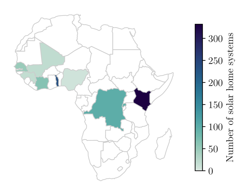
Figure 1: Geographical distribution of the downsampled SHS used in the clustering process. The countries coloured white had no SHS in the dataset.

While BBOXX collect lots of data from their SHSs, for load demand analysis, the time, output current and voltage are the only required time series. The raw data was measured with non-uniform sampling, whereby a measurement is recorded whenever a change is detected, with the associated time stamp of this change also recorded. This is to second resolution, with a 10-minute backstop if no change is detected in that time. To convert this to hourly load demand data, the following method was used:

1. Find instantaneous power $P(t)$ at each time stamp $t$ from the measured voltage $V(t)$ and discharge current $I_{\text{out}}(t)$,

   $$P(t)=V(t)\times I_{\text{out}}(t)$$ (1)

2. Maintain the previous value until the next time stamp (i.e. zero-order hold).

3. Determine the energy consumed by integrating the power. For hourly intervals, $\Delta t=1$ hour,

   $$E(t)=\int_{t-\Delta t}^{t}P(\tau)d\tau$$ (2)

4. Each household is then represented by a discrete energy vector, $E$, where each element is the energy consumed in the respective hour. $t_{end}$ represents the final time step in the time series data.

   $$E_{k}=E(k\cdot\Delta t)\quad\text{where}\quad k\in\left[1,\frac{t_{\text{end}}}{\Delta t}\right]$$ (3)

For each of the 1,000 SHS, a stratified sample based on daily energy consumption was completed to get 10 days representative from each system. From these 10,010 time series, a further energy consumption based stratified sample was taken to get 2,000 time series. This further stratified sampling step was taken because there is not so much dissimilarity in the daily load profiles that it is beneficial to have evermore time series in the clustering problem. Additionally, it is still feasible to cluster using MIP for a dataset of 2,000 which can confirm if a globally optimal solution is found to the clustering problem. Therefore, the clustering exercise was performed on 2,000 time series, each containing 24 values representing hourly load demand for a 24-hour period, starting at midnight.

Once the clustering problem has been solved, the representative centroids are extrapolated to the full dataset, which contains all days for the 1,000 SHSs. To do this, each household is broken down into their daily time series, and each of these daily time series are clustered, using DTW, into the clusters previously found. This gives a chronological sequence of days in each cluster, from the acquisition of the SHS to the time of analysis.

The BBOXX dataset also contains payment data for their customers, extensively analysed in [47]. For this work, the important payment information is the time series of the remaining credit on each SHS. The contracts vary both by location and households’ appliances - households’ energy limits are restricted based on the number of appliances they own, which relates to their tariff. To allow comparison between households, we convert the credit in local currency to the number of days of electricity use remaining on the system. This removes the need for conversion between countries currencies and the different magnitude of payments. Once a household runs out of credit, if it is not topped up again, the system goes into ‘disabled’ state where discharging is not permitted. When a SHS enters this state, it is deemed an economic outage [49].

Finally, we obtain one more metric from the payment data; the utilisation rate. This is defined as the number of days a household is not in economic outage divided by the number of days the household has owned the system. For example, a household with a utilisation rate of 0.9 will be in economic outage on 10% of days since obtaining the SHS. Each household has a utilisation rate calculated for it, at the time of analysis.

IV Clustering Method

This work uses a DTW-MIP clustering software, as described in [50]. The details of the problem formulation can be found in the original paper, but below we present the key ideas here for readability and completeness.

The DTW distance between 2 time series, $x$ and $y$ of length $n$ and $m$, respectively, can be found using dynamic programming:

$$c_{i,j}=(x_{i}-y_{j})^{2}+\min\begin{cases}c_{i-1,j-1}\\ c_{i-1,j}\\ c_{i,j-1}\end{cases}$$ (4)

The final element $c_{n,m}$ is the total DTW distance between $x$ and $y$. In this work, we chose to not use a warping window, which restricts which parts of one time series can be mapped to another [25]. This is because of the benefits of allowing warping along the whole day, allowing similarity to be found between a peak whether it is at night or in the morning. DTW has an implicit penalty for warping, as more warping between two signals means more pairwise comparisons embedded in the final cost. Therefore, while there is an implicit warping penalty, the hard constraint of a warping window is not desirable.

The DTW distance between each time series in the clustering problem is stored in a symmetric matrix $D_{p\times p}$ where $p$ is the number of time series in the clustering problem. A binary square matrix $A_{p\times p}$ is used for the MIP cluster assignment, where $A_{ij}=1$ if time series $j$ is in the cluster with centroid $i$. The clustering optimisation can be solved by

$$A^{\star}=\arg\min_{A}\sum_{i}\sum_{j}D_{ij}\times A_{ij}$$ (5)

To choose the value of $k$ (i.e. the number of clusters), the clustering exercise was done for 2 to 8 clusters. We then compared the costs and silhouette scores [51] to decide on a $k$ value of 5.

V Results and Discussion

The results of this work are divided into three sections. The first section presents representative daily load demand profiles identified through clustering. The second section focuses on the long-term changes in households energy use. This is done in two subsections; the first looks at consumption trends, while the second applies the results of the clustering to the entire dataset, resulting in each household being represented by a series of cluster labels. We examine how each household moves within the cluster space over time, from the initiation of ownership to the time of analysis. The third section considers the payment data and its links to electricity use.

V-A Daily clustering

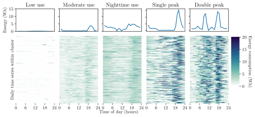
Figure 2: The 5 representative cluster centres from the DTW-MIP clustering of daily SHS load demand profiles, with the heatmaps for all time series within each cluster below. Each heatmap row represents a 24-hour load demand within that cluster. The clusters can be archetypally named: low use, moderate use, nighttime use, single peak and double peak.

Fig. 2 depicts the centroids of the five clusters resulting from the DTW-MIP clustering and the heatmaps for each cluster. The centroids represent the individual time series that minimise the distance between the clusters, as described in the methodology section. Consequently, they can be regarded as the representative time series for the cluster. Nevertheless, it is crucial to examine all the time series within each cluster in order to gain further insight into the discrepancies between the clusters. The heatmaps present each time series within each cluster as a row, with lighter blues representing low energy consumption and darker blues indicating higher energy consumption, which confirms the general agreement between the cluster representatives and their time series.

Table I shows the division of time series in the subset between the clusters, along with the results from the extrapolation of the centres from the subset to the whole dataset. The validity of the extrapolation is shown here, with a larger proportion of time series in the economic outage subset of low use, but generally there is a consistent representation of the full dataset in the subset.

Cluster	Clustering subset			Full dataset
	Count	Proportion	Mean	Count	Proportion	Mean
		of subset	(Wh)		of dataset	(Wh)
Economic outage	-	-	-	118258	0.18	0
Low use	259	0.13	4	39040	0.06	12
Moderate use	583	0.29	42	154765	0.24	39
Nighttime use	573	0.29	69	181696	0.28	73
Single peak	339	0.17	102	86362	0.14	102
Double peak	246	0.12	110	66900	0.10	122

TABLE I: Comparison of the clustering results from the subset, to when the centres are extrapolated to the full dataset.

Cluster	Daily	TV own-	Weekday	Daytime	Appliance
	peaks	ership (%)	use (%)	use (%)	power (W)
Economic outage	0	49	72	N/A	73
Low use	0	48	72	50	71
Moderate use	0.2	17	72	50	50
Nighttime use	0.1	22	71	41	55
Single peak	1.1	84	71	46	96
Double peak	1.9	92	71	59	97
Total population	0.5	43	71	48	68

TABLE II: Mean characteristics of all time series in the dataset, separated into clusters.

Table II shows important characteristics of the time series within each cluster, analysed from the whole dataset, including the peaks in the time series, and information on appliances and time of energy use. A peak within a time series is defined as having double the amplitude of the mean energy consumption of the time series, at least 2 hours apart from another distinct peak (this is to reduce the risk of fluctuations across the threshold counting as two peaks). Additionally, to prevent users with a very small consumption returning lots of peaks due to a very low mean consumption, a peak must have a minimum amplitude of 10W. Defining the cut-off for what is and is not a peak is not rigid, and therefore it is important to also consider the heatmaps in Fig. 2, where the additional peak in the double peak cluster is evident.

Analysing the individualities of each cluster, low use stands out. Given the operational conditions of PAYG systems, this cluster signals two potential scenarios: either there is an economic outage, or there is virtually no usage despite payment. To differentiate between these two states, a new cluster was created, classifying low use time series as economic outage if the time credit balance was 0. It is notable that 24% of days in the dataset belong to economic outage and low use combined, with 75% of them corresponding to economic outages.

The moderate use cluster is a large cluster and has the next lowest mean daily consumption. Looking at the heatmap for this cluster in Fig. 2, the typical use is characterised by consistent low use, with more energy consumed in the evening for most households and a slight increase in use during the morning too. The evening use spans between approximately 3pm to 9pm and therefore crossed over the day/night barrier of 6pm, leading to a non-distinct preference towards daytime or nighttime use. The peak demand is fairly low, and few households within this cluster have TVs, which is reflected in the low mean appliance power. It can be assumed that households with TVs and higher appliance power are not using all their appliances on days when they are in the moderate use cluster.

Nighttime use is another large cluster, with a slightly larger mean daily consumption than moderate use, however there is significant overlap in the daily energy consumption between these two clusters. Nighttime use rate of households TV ownership is low, much like in moderate use, and have a low appliance power of 55 W. The characteristic that distinguishes a time series from being in moderate use or nighttime use, is that nighttime use profiles consume most of their energy at night – between the hours of 6pm and 6am. DTW, as a shape based method, is a very effective measure for picking up discrepancies like this as the shape changes between a generally daytime use profile and nighttime use profile. A nighttime profile will have higher use at the start and end of the time series and lower consumption in the middle, creating a U shape. Whereas the daytime use profile will have lower use at the start and end of the time series with more use somewhere in the middle, creating more of an upside down U shape. The benefit of DTW is the time of peaks, or the beginning/end of the increase or decrease in energy consumption, does not have to align exactly.

The final two clusters are higher consumption days. The mean consumption is marginally higher in double peak, and both clusters have similar rated power appliances. Households in single peak and especially in double peak are very likely to have a TV, which is the main high wattage appliance. However, the difference between these two clusters is the number of peaks. Time series in double peak generally have 2 peaks, while most time series in single peak have only 1. This is seen both in the mean daily peaks in Table II and the heatmaps in Fig. 2. A final distinction between these two higher consumption clusters is that there is a higher proportion of daytime use in double peak, caused by the additional morning peak alongside the evening peak.

Finally, we include the proportion of days in each cluster that are weekdays in Table II to show there is no significant correlation – for each cluster the weekday proportion is around 72% which is the same as the proportion of weekdays to weekend days. This differs to HICs where there is often a noticeable difference in weekday and weekend consumption [52].

Considering all the clusters together, there is a significant non-homogeneity between households energy use, despite the equal technical capabilities of each system with same size battery and solar panel. It can be speculated that the causes of this large variation are financial, or due to the diverse energy needs of different households on different days. However, equipped with this knowledge of the large load demand variation, both on an inter- and intra-household level, it follows that having the same technical specification for each system may be illogical.

V-B Long-term use

V-B1 General consumption trend

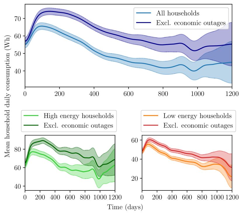
Figure 3: The mean daily household consumption across the SHS initially increases when households first acquire their SHSs, but over time, the consumption decreases. The confidence interval decreases overtime as the number of households in the sample decreases. The bottom subplots split the households into high energy ($>50$ Wh of appliances) and low energy ($\leq 50$ Wh of appliances).

Fig. 3 shows an initial increase in the mean daily consumption, peaking on the 96th day. This initial increase is likely a ‘settling in period’ while the system is getting set up, as well as households purchasing appliances and becoming familiar with the system.

In the first 6 months, daily consumption generally increases for 58% of customers, but by the end of the first year, only 43% of customers continue to increase their energy consumption. Beyond the first year, 77% of users have generally decreasing daily energy consumption since obtaining the system up until the point of data retrieval (between 365 and 1200 days). In absolute terms, the mean energy consumption over two years shows a 33% reduction from its peak, dropping from 66 Wh/day to 44 Wh/day. This is contrary to common thought in literature, which expects energy consumption to increase once access is granted, generally thought to be because users will acquire more appliances and use the system increasing amounts, therefore increasing energy consumption [42]. However, this is not seen here. Instead, SHS users appear to follow a long-term consumption trend similar to that witnessed in their grid-connected counterparts [43].

In the top graph in Fig. 3 we see the general decrease in consumption over time. This is particularly prominent in the first 400 days. Beyond this point, the trend diverges depending on the household. Households are split into high and low energy, based on the summation of all household appliance power. High energy households have appliances that sum to over 50 Wh, while low energy households are equal to or below this.

The high energy households’ mean consumption begins to plateau beyond the 400-day mark, when considering all days. When economic outages are removed from the calculation, there is still a slight decrease in consumption, especially beyond 700 days. Therefore, the stabilisation of the mean consumption is assisted by a decrease in the impact of economic outages beyond this point in high energy households, as well a more consistent consumption when the systems are in use. Another important observation from the high energy subplot is that when economic outages are ignored, the consumption continues to increase until around 250-days of ownership. The decrease in the mean consumption before this time shows a high proportion of economic outages, so when the system is in a use, the consumption increases but the significance of economic outages is so large here that the total mean actually decreases.

In low energy households, the mean relative decrease until the end of the first year is even greater (24%) than in high energy households (12%). The decrease continues, although at a lower rate, until around 800-days. The difference between the mean consumption with and without economic outages in low energy households grows quickly in the first part of ownership and then gradually increases over time.

A decrease in energy use overtime can lead to oversized systems. This is undesirable for many reasons – the solar potential of the system isn’t realised, so there is wasted energy [53, 54], the batteries are not cycling in an optimal manner which can shorten their lifetime [55, 56] and customers are paying for a larger system than they need, increasing the cost of their energy. This is particularly detrimental when the cost of energy is a significant barrier to electrification [57, 46].

V-B2 Cluster space trend

Beyond increasing and decreasing trends, the long-term use for individual households can be analysed by finding an individual households movements within the cluster space over time. From this analysis, an interesting insight is the lack of homogeneity within households. Homogeneity here is defined as the fraction of days a household’s load demand profile is in its dominant cluster (the dominant cluster being the cluster a household is in for the highest number of days). Table III shows the characteristics of households, split into their dominant cluster, including the homogeneity. The mean homogeneity across all households is 55%, so 45% of the days, households aren’t using energy how they ‘typically’ would.

Dominant cluster	Homogen-	Utilisation	TV own-	Flexible	Appliance
	eity (%)	rate (%)	ership (%)	appliances	power (W)
Economic outage	51	48	62	1.4	82
Low use	42	84	53	1.1	72
Moderate use	56	89	8	0.7	44
Nighttime use	61	90	19	0.7	57
Single peak	46	93	91	1.9	102
Double peak	48	92	98	1.8	99

TABLE III: Mean characteristics of households, separated by their dominant cluster – the cluster in which they spend the majority of their time.

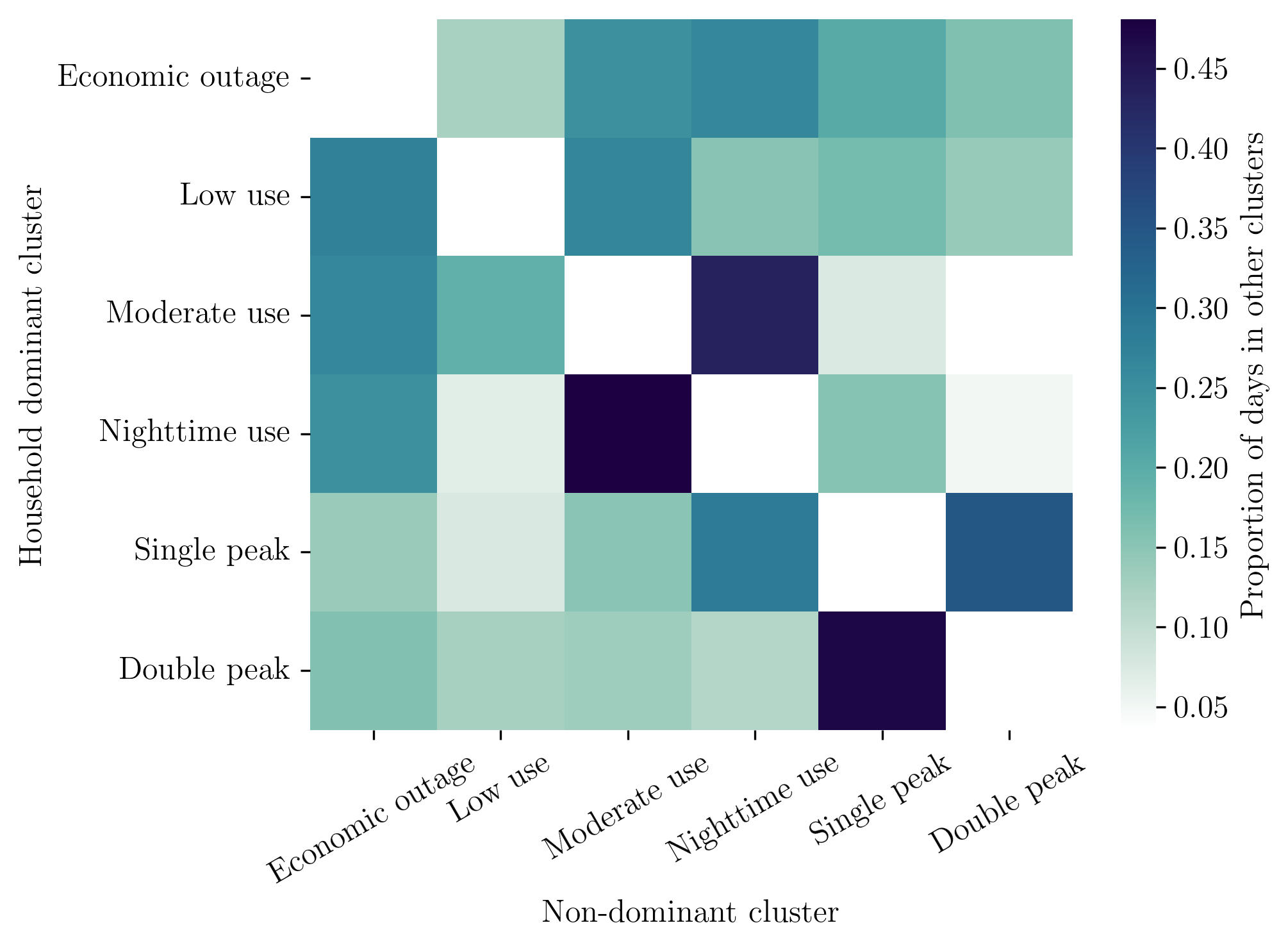
Figure 4: All the households are split into their dominant cluster groups (y-axis). For each of these groups, the spread of days in the other clusters is found (x-axis).

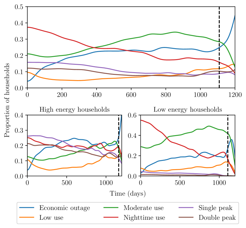
Figure 5: Proportion of households in each cluster, across the lifetime of all the systems (top). The bottom subplots split the households into high energy ($>50$ Wh of appliances) and low energy ($\leq 50$ Wh of appliances). The black dashed line indicates when the number of households in the sample goes below 10.

The higher consumption clusters (single peak and double peak) have lower homogeneity. Table III shows that households with higher consumption dominant clusters, have greater appliance power, with the vast majority of households owning a TV. Therefore, households with higher consumption dominant clusters have the potential to be in all clusters, however, the majority of households with other dominant clusters do not have the potential to consume the energy in the higher consumption clusters due to lack of appliances. Additionally, in the higher consumption clusters, households have more flexible appliances. The base households have lights and phone chargers – these are relatively inflexible loads, as households need lighting when it is dark and to charge phones when the batteries have run out. For this work, we define anything other than lighting and phone charging to be a flexible load. In the higher consumption clusters, households have appliances like TVs and radios which they may not want to use every day, leading to changes in the household energy consumption pattern more often.

Fig. 4 depicts how households, split into their dominant clusters, consume energy when not following their dominant cluster’s behaviour. This further demonstrates the possibility of higher consumption clusters to be in all cluster spaces, whereas is it very uncommon for moderate use households to be in single peak and double peak.

Economic outage is observed in all clusters, but particularly prevalent in the three lower consumption clusters (low use, moderate use and nighttime use). This is logical, as customers who initially pay less for the system have fewer appliances and can be suspected to be more likely to face financial hardship, or be less engaged with the system – both of which lead to missed payments and economic outages.

Beyond the common affinity of all clusters to the economic outage cluster, Fig. 4 shows that clusters with similar magnitude of consumption are more closely linked within households. Households with dominant clusters moderate use and nighttime use are most likely to be in each other’s cluster. Similarly, households with dominant cluster single peak and double peak are most likely to be in each other’s cluster. Therefore, while households energy consumption is clearly non-homogenous, it is more common for households to vary their consumption behaviour within similar magnitudes of use or to not use the system at all and not pay.

Fig. 5 shows the proportion of households in each cluster on each day for the lifetime of the systems. The most important finding is the sharp increase in economic outage over the first year. This is the primary explanation for the reducing electricity consumption, as previously seen in Fig. 3, and shows that customers are reducing engagement with the SHS for economic reasons – either they cannot afford to keep up with payments or they are choosing to not spend their money on SHS credit. Once economic outage begins to level, low use starts to gradually increase. The low use cluster is important for showing when households are choosing to hardly use the system regardless of economic considerations. The increase therefore shows disengagement with the system for non-economic reasons.

Previously, from Fig. 4, the link between nighttime use and moderate use was observed. This link is reinforced in Fig. 5 in the low energy household subplot, where nighttime use significantly reduces over the time of analysis, while moderate use increases. We hypothesise that this is the driver for the decreasing use in low energy households, found in Fig. 3 even when economic outages are ignored. Given their already low consumption levels, the shift from nighttime use to moderate use has a substantial impact. For instance, households might initially use lighting throughout the night for security purposes, but over time, reduce this to only evening hours. To fully understand the reasons behind this behavioural change, further research, including surveys, is necessary.

The high energy household subplot in Fig. 5 shows a similar trend of consistently decreasing single peak and double peak with increase in moderate use and low use. Thus, households are reducing their peak consumption overtime and reducing the use of their flexible loads.

V-C Utilisation rate and electricity use

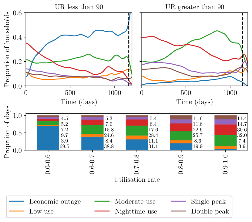
Figure 6: Proportion of households in each cluster over time, split into households with a utilisation rate over 90% and under 90% at time of analysis. The black dashed line indicates when the number of households in the sample goes below 10. The bar chart shows the proportion of days in each cluster for households, grouped by their utilisation rate.

Fig. 5 illustrates a rise in economic outage over time. However, a deeper understanding of household behaviour can be gained by examining utilisation rates. Fig. 6 presents the temporal variation in the proportion of households within each cluster, segmented by utilisation rate. 530 of the households in the dataset have a utilisation rate of 0.9 and above, and only 121 households have a utilisation rate of less than 0.5. Since utilisation rates fluctuate over time, the rate assigned to each household reflects its level at the time of data collection.

The observed increase in economic outage is primarily driven by households with lower utilisation rates, which, by definition, is less evident in households with higher utilisation rates. Beyond economic outages, the cluster space looks different for different utilisation rates, and therefore the utilisation rate influences cluster membership.

In the low utilisation rate group, nighttime use significantly reduces, particularly within the first year. Low use and moderate use fluctuate but stay relatively constant, whereas single peak and double peak steadily decrease. There isn’t a significant increase in any clusters aside from economic outage in the lower utilisation households, so households here are clearly changing their energy behaviour due to financial reasons – either an affordability issue or a lack of desire to spend their money on the system.

For households with higher utilisation rate, the nighttime use continually decreases but at a steadier rate than in lower utilisation households. Higher utilisation rate households are more likely to be in single peak and double peak than lower utilisation rate households. The mean proportion of households in these two highest consumption clusters across the whole timeframe is 19% for low utilisation rate households and 32% for high utilisation households. Thus, households that pay more consistently, are more likely to be in the higher use clusters. However, beyond the first year, single peak and double peak rates decrease, while low use and moderate use increase. The increase in these lower use clusters demonstrates how households are reducing their electricity consumption when economic outage is negligible, which further builds on the previously stated hypothesis of households decreasing electricity consumption while still paying for and engaging with the SHS.

Overall, splitting the households by their utilisation rates draws several key conclusions.

• Energy consumption patterns vary with utilisation rate.

• Economic outage increases significantly over the first year of ownership in low utilisation households. In high utilisation households, the small proportion of economic outages increases gradually over time, peaking at the 3-year mark.

• There is a shift to lower consumption clusters over time, which is more pronounced in households with utilisation rate over 90%.

• Higher consumption clusters are more common in higher utilisation rate households.

VI Conclusion

This work has analysed a large dataset of SHS across sub-Saharan Africa. The DTW-MIP clustering effectively found 5 distinct daily load profiles, archetypal defines as low use, moderate use, nighttime use, single peak and double peak. The representation of these across the dataset shows the SHS is only fully utilised, as in single peak and double peak, on 24% of days – the same proportion of days that the SHS are in economic outage and low use. The majority of time, the SHS provide the basic provisions of moderate use and nighttime use. Households frequently change how they use their SHS, with cluster homogeneity for households averaging 55%. This highlights the importance of granular load demand data, instead of using a one-size-fits-all approach.

Analysis of household behaviour over a period of up to 1,200 days revealed a general decrease in energy consumption among both high and low consumption households. While economic outages are not uncommon under the PAYG scheme, they are not the sole reason for decreasing energy consumption, indicating that changes in energy behaviour extend beyond financial considerations. The decrease in energy consumption when not in economic outage is characterised by a decrease of nighttime energy use, and reduction of days with large evening peaks. Utilisation rates are slightly higher for households that predominantly exhibit single peak and double peak profiles, but even these households—characterised by more flexible appliances and TV ownership, meaning more expensive daily rates—experience economic outages.

Overall, the systems are often underused and therefore oversized, leading to knock-on effects on costs for both households and suppliers. The significant proportion of economic outages suggests that costs remain a limitation for many households, warranting further investigation into how maximising energy provision from each SHS could help reduce the overall cost of energy.

Further work should include surveys of households to understand the underlying causes of the decrease in energy consumption while the systems are still being paid for. Moreover, continuous study of energy behaviour as households gain access to electricity is essential for better understanding their needs and how these evolve over time.

VII Acknowledgements

The authors thank BBOXX for project funding and access to SHS data, and EPSRC for project funding. Prof. Parikh is grateful to the Royal Academy of Engingeering for part funding.

References

- [1] “Goal 7 Department of Economic and Social Affairs.” [Online]. Available: https://sdgs.un.org/goals/goal7
- [2] F. Almeshqab and T. S. Ustun, “Lessons learned from rural electrification initiatives in developing countries: Insights for technical, social, financial and public policy aspects,” pp. 35–53, 3 2019.
- [3] N. Narayan, V. Vega-Garita, Z. Qin, J. Popovic-Gerber, P. Bauer, and M. Zeman, “The long road to universal electrification: A critical look at present pathways and challenges,” Energies, vol. 13, no. 3, 2020.
- [4] Irena, RENEWABLE ENERGY MARKET ANALYSIS AFRICA AND ITS REGIONS, 2022. [Online]. Available: www.afdb.org
- [5] A. H. Pandyaswargo, M. Ruan, E. Htwe, M. Hiratsuka, A. D. Wibowo, Y. Nagai, and H. Onoda, “Estimating the energy demand and growth in off-grid villages: Case studies from Myanmar, Indonesia, and Laos,” Energies, vol. 13, no. 20, 10 2020.
- [6] P. Sandwell, C. Chambon, A. Saraogi, A. Chabenat, M. Mazur, N. Ekins-Daukes, and J. Nelson, “Analysis of energy access and impact of modern energy sources in unelectrified villages in Uttar Pradesh,” Energy for Sustainable Development, vol. 35, pp. 67–79, 12 2016.
- [7] S. Mandelli, M. Merlo, and E. Colombo, “Novel procedure to formulate load profiles for off-grid rural areas,” Energy for Sustainable Development, vol. 31, pp. 130–142, 4 2016.
- [8] P. Boait, R. Gammon, V. Advani, N. Wade, D. Greenwood, and P. Davison, “ESCoBox: A set of tools for mini-grid sustainability in the developing world,” Sustainability (Switzerland), vol. 9, no. 5, 2017.
- [9] P. Boait, V. Advani, and R. Gammon, “Estimation of demand diversity and daily demand profile for off-grid electrification in developing countries,” Energy for Sustainable Development, vol. 29, pp. 135–141, 12 2015.
- [10] C. Blodgett, P. Dauenhauer, H. Louie, and L. Kickham, “Accuracy of energy-use surveys in predicting rural mini-grid user consumption,” Energy for Sustainable Development, vol. 41, pp. 88–105, 12 2017.
- [11] E. Hartvigsson and E. O. Ahlgren, “Comparison of load profiles in a mini-grid: Assessment of performance metrics using measured and interview-based data,” Energy for Sustainable Development, vol. 43, pp. 186–195, 4 2018.
- [12] A. Allee, N. J. Williams, A. Davis, and P. Jaramillo, “Predicting initial electricity demand in off-grid Tanzanian communities using customer survey data and machine learning models,” Energy for Sustainable Development, vol. 62, pp. 56–66, 6 2021.
- [13] M. A. Gelchu, J. Ehnberg, and E. O. Ahlgren, “Comparison Of Electricity Load Estimation Methods In Rural Mini-Grids: Case Study In Ethiopia.” Institute of Electrical and Electronics Engineers (IEEE), 12 2023, pp. 1–5.
- [14] I. Bisaga, N. Puźniak-Holford, A. Grealish, C. Baker-Brian, and P. Parikh, “Scalable off-grid energy services enabled by IoT: A case study of BBOXX SMART Solar,” Energy Policy, vol. 109, pp. 199–207, 2017.
- [15] S. Few, J. Barton, P. Sandwell, R. Mori, P. Kulkarni, M. Thomson, J. Nelson, and C. Candelise, “Electricity demand in populations gaining access: Impact of rurality and climatic conditions, and implications for microgrid design,” Energy for Sustainable Development, vol. 66, pp. 151–164, 2 2022.
- [16] S. C. Bhattacharyya and D. Palit, “A critical review of literature on the nexus between central grid and off-grid solutions for expanding access to electricity in Sub-Saharan Africa and South Asia,” 5 2021.
- [17] T. Den Heeten, N. Narayan, J. C. Diehl, J. Verschelling, S. Silvester, J. Popovic-Gerber, P. Bauer, and M. Zeman, “Understanding the present and the future electricity needs: Consequences for design of future Solar Home Systems for off-grid rural electrification,” in Proceedings of the 25th Conference on the Domestic Use of Energy, DUE 2017. Institute of Electrical and Electronics Engineers Inc., 5 2017, pp. 8–15.
- [18] J. Jurasz, M. Guezgouz, P. E. Campana, and A. Kies, “On the impact of load profile data on the optimization results of off-grid energy systems,” Renewable and Sustainable Energy Reviews, vol. 159, 5 2022.
- [19] S. Yilmaz, J. Chambers, and M. K. Patel, “Comparison of clustering approaches for domestic electricity load profile characterisation - Implications for demand side management,” Energy, vol. 180, pp. 665–677, 8 2019.
- [20] A. Rajabi, M. Eskandari, M. J. Ghadi, L. Li, J. Zhang, and P. Siano, “A comparative study of clustering techniques for electrical load pattern segmentation,” Renewable and Sustainable Energy Reviews, vol. 120, 3 2020.
- [21] Y. Wang, Q. Chen, C. Kang, M. Zhang, K. Wang, and Y. Zhao, “Load Profiling and Its Application to Demand Response: A Review,” Tech. Rep. 2, 2015.
- [22] F. McLoughlin, A. Duffy, and M. Conlon, “A clustering approach to domestic electricity load profile characterisation using smart metering data,” Applied Energy, vol. 141, pp. 190–199, 3 2015.
- [23] U. Von Luxburg and R. C. Williamson, “Clustering: Science or Art?” Tech. Rep., 2012.
- [24] C. Hennig, “What are the true clusters?” Pattern Recognition Letters, vol. 64, pp. 53–62, 10 2015.
- [25] H. Sakoe and S. Chiba, “Dynamic Programming Algorithm Optimization for Spoken Word Recognition,” IEEE Transactions on Acoustics, Speech, and Signal Processing, vol. 26, no. 1, pp. 43–49, 1978.
- [26] S. Lin, F. Li, E. Tian, Y. Fu, and D. Li, “Clustering load profiles for demand response applications,” IEEE Transactions on Smart Grid, vol. 10, no. 2, pp. 1599–1607, 3 2019.
- [27] S. Aghabozorgi, A. Seyed Shirkhorshidi, and T. Ying Wah, “Time-series clustering - A decade review,” Information Systems, vol. 53, pp. 16–38, 5 2015.
- [28] J. R. Ausmus, P. K. Sen, T. Wu, U. Adhikari, Y. Zhang, and V. Krishnan, “Improving the Accuracy of Clustering Electric Utility Net Load Data using Dynamic Time Warping,” in Proceedings of the IEEE Power Engineering Society Transmission and Distribution Conference, vol. 2020-October. Institute of Electrical and Electronics Engineers Inc., 10 2020.
- [29] N. Begum, L. Ulanova, J. Wang, and E. Keogh, “Accelerating dynamic time warping clustering with a novel admissible pruning strategy,” in Proceedings of the ACM SIGKDD International Conference on Knowledge Discovery and Data Mining, vol. 2015-August. Association for Computing Machinery, 8 2015, pp. 49–58.
- [30] C. A. Ratanamahatana and E. Keogh, “Three Myths about Dynamic Time Warping Data Mining.” Proceedings of the 2005 SIAM International Conference on Data Mining (SDM), 2005. [Online]. Available: https://epubs.siam.org/terms-privacy
- [31] T. Teeraratkul, D. O’Neilly, and S. Lallz, “Condensed representation and individual prediction of consumer demand,” in 2016 4th IEEE International Conference on Smart Energy Grid Engineering, SEGE 2016. Institute of Electrical and Electronics Engineers Inc., 10 2016, pp. 11–16.
- [32] V. Kumtepeli, R. Perriment, and D. A. Howey, “DTW-C++: Fast dynamic time warping and clustering of time series data,” Journal of Open Source Software, vol. 9, no. 101, p. 6881, 9 2024. [Online]. Available: https://joss.theoj.org/papers/10.21105/joss.06881
- [33] N. Williams, P. Jaramillo, B. Cornell, I. Lyons-Galante, and E. Wynn, “Load Characteristics of East African Microgrids,” IEEE PES-IAS PowerAfrica Confrence, 2017.
- [34] L. Lorenzoni, P. Cherubini, D. Fioriti, D. Poli, A. Micangeli, and R. Giglioli, “Classification and modeling of load profiles of isolated mini-grids in developing countries: A data-driven approach,” Energy for Sustainable Development, vol. 59, pp. 208–225, 12 2020.
- [35] J. Lukuyu, M. Shiran, R. Kennedy, J. Urpelainen, and J. Taneja, “Purchasing power: Examining customer profiles and patterns for decentralized electricity systems in East Africa,” Energy Policy, vol. 172, 1 2023.
- [36] F. Riva, A. Tognollo, F. Gardumi, and E. Colombo, “Long-term energy planning and demand forecast in remote areas of developing countries: Classification of case studies and insights from a modelling perspective,” pp. 71–89, 4 2018.
- [37] R. Muhumuza, A. Zacharopoulos, J. D. Mondol, M. Smyth, and A. Pugsley, “Energy consumption levels and technical approaches for supporting development of alternative energy technologies for rural sectors of developing countries,” pp. 90–102, 12 2018.
- [38] N. N. Opiyo, “How basic access to electricity stimulates temporally increasing load demands by households in rural developing communities,” Energy for Sustainable Development, vol. 59, pp. 97–106, 12 2020.
- [39] F. Riva, F. D. Sanvito, F. Tonini, and E. Colombo, “Modelling long-term electricity load demand for rural electrification planning; Modelling long-term electricity load demand for rural electrification planning,” Tech. Rep., 2019.
- [40] I. Bisaga and P. Parikh, “To climb or not to climb? Investigating energy use behaviour among Solar Home System adopters through energy ladder and social practice lens,” Energy Research and Social Science, vol. 44, pp. 293–303, 10 2018.
- [41] V. Kizilcec, C. Spataru, A. Lipani, and P. Parikh, “Forecasting Solar Home System Customers’ Electricity Usage with a 3D Convolutional Neural Network to Improve Energy Access,” Energies, vol. 15, no. 3, 2 2022.
- [42] C. Dominguez, K. Orehounig, and J. Carmeliet, “Understanding the path towards a clean energy transition and post-electrification patterns of rural households,” Energy for Sustainable Development, vol. 61, pp. 46–64, 4 2021.
- [43] L. Masselus, J. Ankel-Peters, G. Gonzalez Sutil, V. Modi, J. Mugyenyi, A. Munyehirwe, N. Williams, and M. Sievert, “10 Years After: Long-term Adoption of Electricity in Rural Rwanda,” Tech. Rep., 2024.
- [44] H. Louie, S. Atcitty, D. Terry, D. Lee, and P. Romine, “Daily electrical energy consumption characteristics and design implications for off-grid homes on the Navajo Nation,” Energy for Sustainable Development, vol. 73, pp. 315–325, 4 2023.
- [45] M. P. Blimpo, A. Postepska, and Y. Xu, “Why is household electricity uptake low in Sub-Saharan Africa?” World Development, vol. 133, 9 2020.
- [46] V. Kizilcec and P. Parikh, “Solar Home Systems: A comprehensive literature review for Sub-Saharan Africa,” pp. 78–89, 10 2020.
- [47] V. P. Mergulhão, L. Capra, K. Voglitsis, and P. Parikh, “How do they pay as they go?: Learning payment patterns from solar home system users data in Rwanda and Kenya,” Energy for Sustainable Development, vol. 76, 10 2023.
- [48] J. A. Guajardo, “How Do Usage and Payment Behavior Interact in Rent-to-Own Business Models? Evidence from Developing Economies,” Production and Operations Management, vol. 28, no. 11, pp. 2808–2822, 11 2019.
- [49] I. Ferrall, D. Callaway, and D. M. Kammen, “Measuring the reliability of SDG 7: The reasons, timing, and fairness of outage distribution for household electricity access solutions,” Environmental Research Communications, vol. 4, no. 5, 5 2022.
- [50] V. Kumtepeli, R. Perriment, and D. A. Howey, “Fast dynamic time warping and clustering in C++,” 7 2023. [Online]. Available: http://arxiv.org/abs/2307.04904
- [51] K. R. Shahapure and C. Nicholas, “Cluster quality analysis using silhouette score,” in Proceedings - 2020 IEEE 7th International Conference on Data Science and Advanced Analytics, DSAA 2020. Institute of Electrical and Electronics Engineers Inc., 10 2020, pp. 747–748.
- [52] G. Trotta, “An empirical analysis of domestic electricity load profiles: Who consumes how much and when?” Applied Energy, vol. 275, 10 2020.
- [53] S. Bhatti and A. Williams, “Estimation of surplus energy in off-grid solar home systems,” Renewable Energy and Environmental Sustainability, vol. 6, p. 25, 2021.
- [54] B. Soltowski, D. Campos-Gaona, S. Strachan, and O. Anaya-Lara, “Bottom-up electrification introducing new smart grids architecture-concept based on feasibility studies conducted in Rwanda,” Energies, vol. 12, no. 12, 2019.
- [55] N. Narayan, A. Chamseddine, V. Vega-Garita, Z. Qin, J. Popovic-Gerber, P. Bauer, and M. Zeman, “Exploring the boundaries of Solar Home Systems (SHS) for off-grid electrification: Optimal SHS sizing for the multi-tier framework for household electricity access,” Applied Energy, vol. 240, pp. 907–917, 4 2019.
- [56] R. Perriment, V. Kumtepeli, M. McCulloch, and D. Howey, “Lead-Acid Battery Lifetime Extension in Solar Home Systems Under Different Operating Conditions.” Institute of Electrical and Electronics Engineers (IEEE), 12 2023, pp. 1–5.
- [57] F. Kyere, S. Dongying, G. D. Bampoe, N. Y. G. Kumah, and D. Asante, “Decoding the shift: Assessing household energy transition and unravelling the reasons for resistance or adoption of solar photovoltaic,” Technological Forecasting and Social Change, vol. 198, 1 2024.