MAGNETIC THOMSON TRANSPORT IN HIGH OPACITY DOMAINS

Abstract

X-ray radiation from neutron stars manifests itself in a variety of settings. Isolated pulsars, and magnetars both exhibit quasi-thermal persistent soft X-ray emission from their surfaces. Transient magnetospheric bursts from magnetars and pulsed signals from accreting neutron stars mostly appear in harder X rays. The emission zones pertinent to these signals are all highly Thomson optically thick so that their radiation anisotropy and polarization can be modeled using sophisticated simulations of scattering transport from extended emission regions. Validation of such codes and their efficient construction is enhanced by a deep understanding of scattering transport in high opacity domains. This paper presents a new analysis of the polarized magnetic Thomson radiative transfer in the asymptotic limit of high opacity. The integro-differential equations for photon scattering transport that result from a phase matrix construction are reduced to a compact pair of equations. This pair is then solved numerically for two key parameters that describe the photon anisotropy and polarization configuration of high Thomson opacity environs. Empirical approximations for these parameters as functions of the ratio of the photon and cyclotron frequencies are presented. Implementation of these semi-analytic transport solutions as interior boundary conditions is shown to speed up scattering simulations. The solutions also enable the specification of the anisotropic radiation pressure. The analysis is directly applicable to the atmospheres of magnetars and moderate-field pulsars, and to the accretion columns of magnetized X-ray binaries, and can be adapted to address other neutron star settings.

1 Introduction

Compton scattering has long been invoked in a variety of contexts for neutron star emission, spanning their pulsed surface X-ray luminosity to their persistent and transient hard X-ray signals emanating from their magnetospheres. Central to considerations in the emission zones is the anisotropy imposed by the strong magnetic fields of neutron stars. These fields are typically around a TeraGauss, yet span a broad range from around 1 GigaGauss for millisecond pulsars (see the ATNF Pulsar Catalogue) to 1 PetaGauss for magnetars (see the McGill Magnetar Catalog (Olausen & Kaspi, 2014) and its online portal), naturally placing the electron cyclotron frequency $\,\omega_{\hbox{\fiverm B}}\,$ in the X-ray or gamma-ray band. In these domains, the resonance in the cross section that naturally arises at the cyclotron frequency (Canuto et al., 1971; Herold, 1979) and its harmonics (Daugherty & Harding, 1986) strongly impacts the character of scattering anisotropy and polarization levels in optically thick environs.

Principal astrophysical environments where such cyclotron resonance influences are important include accreting X-ray binaries such as Her X-1, 4U 0115+63, Vela X-1 and AO 0535+26. Cyclotron absorption features have been observed above around 10 keV in about three dozen systems (see the review by Staubert et al., 2019), and are used to calibrate their magnetic fields to the $\,\mathrel{\mathchoice{\lower 2.0pt\vbox{\halign{$\m@th\displaystyle\hfil#\hfil$\cr>\crcr\sim\crcr}}}{\lower 2.0pt\vbox{\halign{$\m@th\textstyle\hfil#\hfil$\cr>\crcr\sim\crcr}}}{\lower 2.0pt\vbox{\halign{$\m@th\scriptstyle\hfil#\hfil$\cr>\crcr\sim\crcr}}}{\lower 2.0pt\vbox{\halign{$\m@th\scriptscriptstyle\hfil#\hfil$\cr>\crcr\sim\crcr}}}}10^{12}\,$Gauss domain (e.g., Trümper et al., 1978; Coburn et al., 2002). The leading interpretation is that these features are generated through scattering and absorption at the cyclotron resonances in their accretion columns at or just above the stellar surface. The line detections have led to sophisticated codes modeling radiative transfer and the accompanying formation of spectral lines (e.g., Isenberg et al., 1998; Araya & Harding, 1999; Schönherr et al., 2007; Schwarm et al., 2017). These Thomson optically thick columns are funnels of infalling material collimated by the magnetic field lines above the polar surface regions.

Surface signals from isolated pulsars and magnetic white dwarfs are also subject to strong cyclotronic influences on radiation emanating from their high opacity atmospheres. In the case of white dwarfs, the character of anisotropy and polarization due to atmospheric magnetic Thomson scattering was explored using Monte Carlo simulations by Whitney (1991). Yet the white dwarf context is complicated by the presence of numerous atomic lines and mixtures in the atmospheric composition: see Wickramasinghe & Ferrario (2000) for a review, and Jewett et al. (2024) for a Gaia-era spectroscopic update. The modeling of surface X-ray emission from neutron stars has received extensive treatment over the years. Most studies use scattering and free-free opacity to mediate the photon transport and also help support the atmospheres hydrostatically. Older investigations focused on traditional neutron stars with surface polar fields $\,B_{p}<10^{13}\,$Gauss, mostly fully-ionized hydrogen/helium atmospheres at temperatures $\,T\sim 10^{6}\,$K (Shibanov et al., 1992; Pavlov et al., 1994; Zavlin et al., 1996; Zane et al., 2000).

A more recent focus has been on atmospheric emission from magnetars. This has primarily been because they are hot and therefore bright, and so are easily observable at distance of 10 kpc or more. Their surface polar field strengths are typically in the range of $\,10^{14}-2\times 10^{15}\,$Gauss, placing the electron cyclotron frequency $\,\omega_{\hbox{\fiverm B}}\,$ in the gamma-ray band. Accordingly, there is a strong suppression of the scattering cross section in the X-ray band (Canuto et al., 1971; Herold, 1979), particularly for one of the polarization eigenmodes. This effect critically influences the scattering process and emergent polarization from magnetar atmospheres, and has been explored at length using solutions of the radiative transfer equation by various groups (Ho & Lai, 2001; Özel, 2001; Ho & Lai, 2003; Özel, 2003; van Adelsberg & Lai, 2006; Taverna et al., 2015), mostly using semi-analytic, Feautrier-type techniques. Their analyses included detailed treatment of the polarization of the vacuum by the strong magnetic field (Tsai & Erber, 1975), an influence of quantum electrodynamics (QED) that renders the vacuum birefringent so that radiative transfer is sensitive to the polarization state (mode), just as it is for a plasma. There have also been Monte Carlo simulations of atmospheric radiative transport (Bulik & Miller, 1997; Niemiec & Bulik, 2006; Barchas et al., 2021; Hu et al., 2022) that enable great facility in treating various surface locales possessing different B orientations to the zenith direction.

Magnetars also exhibit sporadic and highly super-Eddington burst emission, so luminous that their radiating plasma densities are optically thick to Compton scattering (e.g., Taverna & Turolla, 2017). This leads to the appearance of broad, non-thermal “Comptonized” hard X-ray spectra (e.g. Lin et al., 2011, 2012; Younes et al., 2014). Consequently, the intense radiation pressure in magnetar bursts (and even more so in the much rarer giant flares) must push the emitting plasma so that it moves relativistically within the burst emission regions. The speeds of the motions are governed by radiation-driven dynamics, which will influence the spectrum of the radiation we observe (Lin et al., 2012; Roberts et al., 2021), and undoubtedly its polarization also. Therefore, understanding the dependence of (polarized) radiation pressure on anisotropies induced by Compton scattering in the strong magnetic field is an important element of constructing realistic emission models for magnetar bursts and giant flares.

A deeper appreciation of magnetic scattering transport in high opacity domains is therefore warranted, both to enhance the definition of boundary conditions for radiative transfer computations and transport simulations of emission regions that are highly magnetized, and also to improve the understanding of the associated pressure anisotropy of the radiation field. This is most conveniently delivered in the regime of magnetic Thomson scattering, for which the cross section is mathematically simple, and is not imbued with the complexities of QED modifications, which include a multitude of resonant cyclotron harmonics. Yet the magnetic Thomson domain is quite broadly applicable to white dwarfs in general, and to soft X-ray surface emission below 5 keV from neutron stars of different varieties, ranging from millisecond pulsars to Crab-like pulsars to magnetars; QED influences in strong fields (e.g. Daugherty & Harding, 1986) generally only become important for photon energies $\,\mathrel{\mathchoice{\lower 2.0pt\vbox{\halign{$\m@th\displaystyle\hfil#\hfil$\cr>\crcr\sim\crcr}}}{\lower 2.0pt\vbox{\halign{$\m@th\textstyle\hfil#\hfil$\cr>\crcr\sim\crcr}}}{\lower 2.0pt\vbox{\halign{$\m@th\scriptstyle\hfil#\hfil$\cr>\crcr\sim\crcr}}}{\lower 2.0pt\vbox{\halign{$\m@th\scriptscriptstyle\hfil#\hfil$\cr>\crcr\sim\crcr}}}}20\,$keV.

This paper presents a new analysis of the polarized magnetic Thomson radiative transfer in the asymptotic limit of high opacity. The approach obtains solutions of the polarized radiation transport integro-differential equations, leveraging the simplicity of the magnetic Thomson differential cross section (Canuto et al., 1971; Herold, 1979). In Sec. 2, the system is distilled down to two integral equations that constitute a transcendental system. These are then solved numerically in Sec. 3 for the two key parameters that describe the photon anisotropy and polarization configuration of high opacity environs. After isolating analytic solutions in low and high frequency domains in Sec. 3.1, empirical approximations for these two parameters as functions of the ratio of the photon and cyclotron frequencies are developed in Sec. 3.2. The Stokes parameter variations and resultant pressure anisotropies are addressed in Sec. 3.3. Implementation of the semi-analytic transport solutions as interior boundary conditions in atmospheric slabs is shown in Sec. 4 to speed up the magnetic Thomson scattering simulations of Barchas et al. (2021); Hu et al. (2022). The discussion therein highlights the broader applicability of the results to neutron star settings.

2 Magnetic Thomson Transport using a Phase Matrix Approach

The determination of the configuration of radiation anisotropy and polarization in magnetized plasmas can be addressed by standard radiative transfer techniques such as in Chandrasekhar (1960). It can also be approached using Monte Carlo simulation techniques, as it was in Barchas et al. (2021) and Hu et al. (2022). Via either protocol, deep in the radiative transport environment, the radiation field realizes an asymptotic equilibrium wherein single scatterings do not change the distributions of photon angles and polarizations. This is the domain that is addressed here in deriving both analytic and numerical descriptions of the asymptotic radiation configuration. Throughout the paper, the magnetic field $\,\boldsymbol{B}\,$ threading the radiative transfer region is presumed uniform on scales much larger than the scattering mean free path.

To determine the asymptotic state, it is necessary to include all information about polarizations and their interchange in scattering events. To effect this, in this paper we employ the phase matrix approach for the 4 familiar Stokes parameters, $\,I,Q,U,V\,$. Here, $\,I\,$ represents the intensity, $\,Q,U\,$ define the linear polarization degree and angle configuration, and $\,V\,$ pertains to circular polarization. The equilibrium configuration is established via a redistribution function $\,{\cal P}/\sigma\,$ (to be defined) that specifies the probability of redistribution in angles and polarization states under the operation of magnetic Thomson scattering. The analysis is constructed using the $\,4\times 4\,$ phase matrix approach of Chou (1986) that describes the mappings in Stokes parameter space in scatterings. Such mappings correspond to dipole radiation by electrons gyrating in the magnetic field in response to the Newton-Lorentz force provided by the incoming electromagnetic wave. This classical description of magnetic Thomson scattering was first presented by Canuto et al. (1971). Exploiting the azimuthal symmetry of the uniform magnetic field problem, without loss of generality we will eventually set $\,U=0\,$ and average over azimuthal angles (phases) about $\,\boldsymbol{B}\,$.

2.1 Radiative Transfer Set-up

The photon wavenumber $\,\boldsymbol{k}\,$ (momentum/$\hbar$) will be described via polar $\,(k,\,\theta,\,\phi)\,$ coordinates in between scatterings, with $\,\theta=\arccos(\hat{\boldsymbol{k}}\cdot\hat{\boldsymbol{B}})\,$ being the polar angle relative to the field direction $\,\hat{\boldsymbol{B}}\,$, and $\,\phi\,$ being the azimuthal angle around the field. In an unpolarized system, only the intensity $\,I\,$ comes into consideration, and the radiative transfer equation assumes the form

$$\hbox{${{\displaystyle 1\vphantom{(}}\over{\displaystyle c\vphantom{(}}}$}\,\hbox{${{\displaystyle dI\vphantom{(}}\over{\displaystyle dt\vphantom{(}}}$}\;=\;-n_{e}\sigma(\boldsymbol{k})\,I(\boldsymbol{k})+n_{e}\int\hbox{${{\displaystyle d\sigma(\boldsymbol{k}_{i}\to\boldsymbol{k})\vphantom{(}}\over{\displaystyle d\Omega\vphantom{(}}}$}\,I(\boldsymbol{k}_{i})\,d\Omega_{i}\quad.$$ (1)

Here, $\,n_{e}\,$ is the electron number density, and the differential cross section $\,d\sigma/d\Omega\,$ and accompanying total cross section are detailed in Canuto et al. (1971); see also Herold (1979) for the mathematically equivalent quantum version of the magnetic Thomson cross section. The first term on the right of Eq. (1) represents the rate of loss of photons from a given wavenumber bin $\,\boldsymbol{k}\,$. The second term on the right defines the rate of gain in a wavenumber bin, and integrates over all the directions $\,d\Omega_{i}=d(\cos\theta_{i})\,d\phi_{i}\,$ of the initial (pre-scattering) photons $\,\boldsymbol{k}_{i}\,$; the subscript for the final photon is dropped. For equilibrium in high opacity domains, the intensity is invariant, and so the left hand side is zero. Note that as the opacity increases, the approach to equilibrium is not uniform in either direction or polarization due to the pathology of the cross section. This is the focal regime of this paper, leading to the equality

$$\sigma(\boldsymbol{k})\,I(\boldsymbol{k})\;=\;\int\hbox{${{\displaystyle d\sigma(\boldsymbol{k}_{i}\to\boldsymbol{k})\vphantom{(}}\over{\displaystyle d\Omega\vphantom{(}}}$}\,I(\boldsymbol{k}_{i})\,d\Omega_{i}\quad.$$ (2)

The specific mathematical form of the magnetic Thomson cross section then determines the angular dependence of the intensity up to an unconstrained normalization. This steady-state identity is appropriate for intensity evolution in a highly optically-thick plasma, and can routinely be adapted to introduce the photon polarization dependence.

Let $\,\boldsymbol{S}=(I,Q,U,V)\equiv(S_{1},S_{2},S_{3},S_{4})\,$ be the true Stokes vector of the photon field that can be represented using the Poincaré sphere. Using the complex vector representation of photon electric fields (polarizations) in Barchas et al. (2021), this Stokes vector can be written as

$$\boldsymbol{S}\;\equiv\;\left(\begin{array}[]{c}I\\[2.0pt] Q\\[2.0pt] U\\[2.0pt] V\end{array}\right)\;=\;\left(\begin{array}[]{c}\langle{\cal E}_{\theta}{\cal E}_{\theta}^{*}\rangle+\langle{\cal E}_{\phi}{\cal E}_{\phi}^{*}\rangle\\[2.0pt] \langle{\cal E}_{\theta}{\cal E}_{\theta}^{*}\rangle-\langle{\cal E}_{\phi}{\cal E}_{\phi}^{*}\rangle\\[2.0pt] \langle{\cal E}_{\theta}{\cal E}_{\phi}^{*}\rangle+\langle{\cal E}_{\theta}^{*}{\cal E}_{\phi}\rangle\\[2.0pt] i\,\langle{\cal E}_{\theta}{\cal E}_{\phi}^{*}-{\cal E}_{\theta}^{*}{\cal E}_{\phi}\rangle\end{array}\right)\quad\hbox{with}\quad\boldsymbol{\cal E}\;=\;{\cal E}_{\theta}\hat{\theta}+{\cal E}_{\phi}\hat{\phi}\;\equiv\;\bigl{|}\boldsymbol{\cal E}\bigr{|}\bigl{(}\hat{\cal E}_{\theta}\hat{\theta}+\hat{\cal E}_{\phi}\hat{\phi}\bigr{)}$$ (3)

as the polarization vector in our polar coordinate specification. The brackets $\,\langle\dots\rangle\,$ signify time averages of the products of wave field components; the Stokes parameters can be summed over any number of photons. One can also form a reduced Stokes parameter 3-vector $\,\hat{\boldsymbol{S}}=(\hat{Q},\,\hat{U},\,\hat{V})\equiv(Q/I,\,U/I,\,V/I)\,$ using the intensity to scale the other polarization quantities of interest. It then follows that $\,|{\hat{Q}}|\leq 1\,$ and similarly for $\,{\hat{U}},{\hat{V}}\,$.

Then extension of the radiative transfer equilibrium equation in Eq. (2) to treat polarized systems leads to the high opacity asymptotic identity

$$\sigma(\boldsymbol{k})\,\boldsymbol{S}(\boldsymbol{k})\;=\;\sum_{i,f=1,4}\int\hbox{${{\displaystyle d\sigma_{i\to f}(\boldsymbol{k}_{i}\to\boldsymbol{k})\vphantom{(}}\over{\displaystyle d\Omega\vphantom{(}}}$}\,\boldsymbol{S}(\boldsymbol{k}_{i})\,d\Omega_{i}\quad.$$ (4)

Here $\,i\to f\,$ represents the polarization transition in scattering from one initial photon polarization state $\,i\,$ to a final one $\,f\,$. Thus $\,i,f=1\to 4\,$ map through the Stokes parameters $\,I,Q,U,V\,$ in sequence. This is a vector equation and the differential cross section is now a $\,4\times 4\,$ matrix, i.e. a tensor. The transfer equation can also be cast in a form that uses the $\,4\times 4\,$ polarization phase matrix $\,\mathbf{P}\,$ with 16 elements $\,P_{if}\,$:

$$\sigma(\boldsymbol{k})\,\boldsymbol{S}(\boldsymbol{k})\;=\;\int\mathbf{P}(\boldsymbol{k}_{i}\to\boldsymbol{k})\,\Bigl{[}\sigma(\boldsymbol{k}_{i})\,\boldsymbol{S}(\boldsymbol{k}_{i})\Bigr{]}\,d\Omega_{i}\quad,\quad P_{if}\;=\;\hbox{${{\displaystyle 1\vphantom{(}}\over{\displaystyle\sigma(\boldsymbol{k}_{i})\vphantom{(}}}$}\,\hbox{${{\displaystyle d\sigma_{i\to f}(\boldsymbol{k}_{i}\to\boldsymbol{k})\vphantom{(}}\over{\displaystyle d\Omega\vphantom{(}}}$}\;\equiv\;\hbox{${{\displaystyle r_{0}^{2}\,\hat{P}_{if}\vphantom{(}}\over{\displaystyle\sigma(\boldsymbol{k}_{i})\vphantom{(}}}$}\quad,$$ (5)

Accordingly, $\,\sigma(\boldsymbol{k})\,\boldsymbol{S}(\boldsymbol{k})\,$ is an eigenvector of the phase matrix. The scaled versions $\,\hat{P}_{if}\,$ of the phase matrix elements are introduced here to isolate their common cross section normalization. Note that $\,r_{0}=e^{2}/(m_{e}c^{2})\,$ is the classical electron radius, from which one derives the total non-magnetic Thomson cross section $\,\sigma_{\hbox{\sixrm T}}=8\pi r_{0}^{2}/3\,$.

The Stokes vector $\,\boldsymbol{S}(\boldsymbol{k})\,$ depends on the direction of the radiation relative to $\,\boldsymbol{B}\,$, thereby expressing its anisotropy. The cross section $\,\sigma(\boldsymbol{k})\,$ now depends on the polarization configuration, and therefore implicitly on $\,\boldsymbol{S}(\boldsymbol{k})\,$. Eq. (13) of Barchas et al. (2021) presents the form

$$\sigma(\boldsymbol{k})\;=\;\sigma_{\hbox{\sixrm T}}\biggl{\{}\Sigma_{\hbox{\sixrm B}}(\omega)\,\hat{I}(\boldsymbol{k})+\hbox{${{\displaystyle 1\vphantom{(}}\over{\displaystyle 2\vphantom{(}}}$}\Bigl{[}1-\Sigma_{\hbox{\sixrm B}}(\omega)\Bigr{]}\Bigl{\{}\hat{I}(\boldsymbol{k})+\hat{Q}(\boldsymbol{k})\Bigr{\}}\,\bigl{(}1-\mu^{2}\bigr{)}+\Delta_{\hbox{\sixrm B}}(\omega)\,\hat{V}(\boldsymbol{k})\,\mu\biggr{\}}$$ (6)

for the polarized magnetic Thomson cross section, where $\,\mu=\cos\theta\,$ is the angle cosine of the initial photon, and $\,\sigma_{\hbox{\sixrm T}}\,$ is the Thomson cross section. As above, the hat notation signifies $\,\hat{Q}=Q/I\,$, etc, so that $\,\hat{I}=1\,$. Two functions appear that depend only on the photon frequency $\,\omega=c/|\boldsymbol{k}|\,$:

$$\Sigma_{\hbox{\sixrm B}}(\omega)=\hbox{${{\displaystyle\omega^{2}(\omega^{2}+\omega_{\hbox{\fiverm B}}^{2})\vphantom{(}}\over{\displaystyle(\omega^{2}-\omega_{\hbox{\fiverm B}}^{2})^{2}\vphantom{(}}}$}\;=\;\hbox{${{\displaystyle 1\vphantom{(}}\over{\displaystyle 2\vphantom{(}}}$}\biggl{\{}\hbox{${{\displaystyle\omega^{2}\vphantom{(}}\over{\displaystyle(\omega-\omega_{\hbox{\fiverm B}})^{2}\vphantom{(}}}$}+\hbox{${{\displaystyle\omega^{2}\vphantom{(}}\over{\displaystyle(\omega+\omega_{\hbox{\fiverm B}})^{2}\vphantom{(}}}$}\biggr{\}}\;,\quad\Delta_{\hbox{\sixrm B}}(\omega)=\hbox{${{\displaystyle 2\omega^{3}\omega_{\hbox{\fiverm B}}\vphantom{(}}\over{\displaystyle(\omega^{2}-\omega_{\hbox{\fiverm B}}^{2})^{2}\vphantom{(}}}$}\;=\;\hbox{${{\displaystyle 1\vphantom{(}}\over{\displaystyle 2\vphantom{(}}}$}\biggl{\{}\hbox{${{\displaystyle\omega^{2}\vphantom{(}}\over{\displaystyle(\omega-\omega_{\hbox{\fiverm B}})^{2}\vphantom{(}}}$}-\hbox{${{\displaystyle\omega^{2}\vphantom{(}}\over{\displaystyle(\omega+\omega_{\hbox{\fiverm B}})^{2}\vphantom{(}}}$}\biggr{\}}$$ (7)

that can be termed the linearity and circularity functions, respectively. They depend only on the ratio of the photon frequency $\,\omega\,$ to the electron cyclotron frequency $\,\omega_{\hbox{\fiverm B}}=eB/(m_{e}c)\,$, and therefore are not independent functions. The combination of angle and polarization dependence within $\,\sigma(\boldsymbol{k})\,$ guarantees an intricate and frequency-dependent interplay between polarization and anisotropy in the transport of photons in a magnetized plasma. Eq. (6) agrees with Eq. (4) of Whitney (1991) and Eq. (2.26) of Barchas (2017), both of which were derived from the polarization phase matrix analysis of Chou (1986). Note that in the limit of small fields, i.e. $\,\omega\gg\omega_{\hbox{\fiverm B}}\,$, then $\,\Sigma_{\hbox{\sixrm B}}\to 1\,$ and $\,\Delta_{\hbox{\sixrm B}}\to 0\,$, and Eq. (6) reduces to the familiar non-magnetic Thomson result: the cross section is then independent of the magnetic field and the photon direction.

2.2 Reduction of the System of Transport Equations

The algebraic expressions that Chou (1986) developed for the differential cross section are long and complicated in terms of their dependence on the polar angles $\,\theta_{i,f}\,$ and azimuthal/phase ones $\,\phi_{i,f}\,$. Moreover, they are then specialized to the case of a phase angle difference $\,\phi_{fi}=\phi_{f}-\phi_{i}=0\,$, which does not capture all the required information for the radiative transfer analysis. Accordingly, we use as our starting point the modified version posited in Eq. (2) of Whitney (1991); see also Eq. (2.24) and subsequent equations on pages 42-43 of Barchas (2017). While Chou (1986) formed a representation of the phase matrix using the true Stokes vectors $\,\boldsymbol{S}\,$, Whitney (1991) noted that it proved algebraically more convenient to employ the decomposition $\,I=I_{\parallel}+I_{\perp}\,$ and $\,Q=I_{\parallel}-I_{\perp}\,$ and work with $\,I_{\parallel,\perp}\,$. This amounts to a simple rotation in the $\,(S_{1},S_{2})\,$ elements that can be applied to the phase matrix/tensor. By inspection of the Stokes parameter definitions in Eq. (3), one quickly discerns that $\,I_{\parallel}=\langle{\cal E}_{\theta}{\cal E}_{\theta}^{*}\rangle\,$ and so contains information about electric field components in the $\,\boldsymbol{k}-\boldsymbol{B}\,$ plane. Thus, $\,I_{\parallel}\,$ represents the intensity of the $\,\parallel\,$ linear polarization component, the so-called ordinary mode. Similarly, $\,I_{\perp}=\langle{\cal E}_{\phi}{\cal E}_{\phi}^{*}\rangle\,$ only contains information on electric field components perpendicular to the $\,\boldsymbol{k}-\boldsymbol{B}\,$ plane, and thus defines the intensity of the $\,\perp\,$ linear polarization (extraordinary mode). After an appropriate amount of algebraic development, eventually we will revert to the Chou representation for aesthetic reasons that will shortly become apparent.

Accordingly, we seek to algebraically develop the equilibrium integral equation problem

$$\boldsymbol{\Lambda}(\boldsymbol{k})\;=\;\int\mathbf{P}(\boldsymbol{k}_{i}\to\boldsymbol{k})\,\boldsymbol{\Lambda}(\boldsymbol{k}_{i})\,d\Omega_{i}\quad,\quad\boldsymbol{\Lambda}(\boldsymbol{k})\;\equiv\;\sigma(\boldsymbol{k})\,\boldsymbol{S}(\boldsymbol{k})\quad,$$ (8)

with $\,\boldsymbol{S}\to(I_{\parallel},\,I_{\perp},\,U,\,V)\,$, and reduce it in preparation for numerical solution. The first step is to adopt a random phase approximation. At high opacity, uniformity in azimuthal “phase” $\,\phi\,$ about $\,\boldsymbol{B}\,$ should be realized because the differential cross section has no peculiar dependence on the azimuthal angles; i.e. the configuration is invariant under rotations about $\,\boldsymbol{B}\,$. This then applies to both $\,\boldsymbol{S}\,$ and also $\,\boldsymbol{\Lambda}\,$, since $\,\sigma(\boldsymbol{k})\,$ has no explicit dependence on azimuth. Thus, $\,\boldsymbol{\Lambda}(\boldsymbol{k})\to\boldsymbol{\Lambda}(\omega,\,\mu)\,$, for photon frequency $\,\omega\,$ and propagation angle cosine $\,\mu=\cos\theta\,$ relative to $\,\boldsymbol{B}\,$, and we shall employ the $\,\sigma(\boldsymbol{k})\to\sigma(\omega,\,\mu)\,$ correspondence in what follows. Also, without loss of generality (WLOG), one can choose polar coordinates so that the Stokes U is zero and Stokes Q provides the only contribution to the linear polarization. This is tantamount to an orientation of the polar axis along $\,\boldsymbol{B}\,$ and a particular choice for the zero of the azimuthal angle coinciding with the $\,\boldsymbol{k}-\boldsymbol{B}\,$ plane. This sets 7 elements of the phase matrix to be zero. With this simplification, the system can be expressed using $\,3\times 3\,$ reduced phase matrix $\,\mathbf{P}_{\rm red}\,$. The transport equilibrium is then expressed via

$$\boldsymbol{\Lambda}_{\parallel,\perp}(\omega,\,\mu)\;=\;\int_{-1}^{1}{\cal R}(\mu_{i},\mu)\,\boldsymbol{\Lambda}_{\parallel,\perp}(\omega,\,\mu_{i})\,d\mu_{i}\quad\hbox{with}\quad\boldsymbol{\Lambda}_{\parallel,\perp}(\omega,\,\mu)\;=\;\sigma(\omega,\,\mu)\left(\begin{array}[]{c}I_{\parallel}\\ I_{\perp}\\ V\\ \end{array}\right)\;\equiv\;\left(\begin{array}[]{c}\Lambda_{\parallel}(\omega,\,\mu)\\ \Lambda_{\perp}(\omega,\,\mu)\\ \Lambda_{V}(\omega,\,\mu)\\ \end{array}\right)\;\;,$$ (9)

constituting a three-dimensional eigenvalue/eigenvector problem. Observe that in Eq. (9), the angle cosine $\,\mu\,$ represents that for the final (scattered) photon on the right hand side, and the initial pre-scattering photon on the left side. The subscript $\,\parallel,\perp\,$ marks that this applies to the Whitney (1991) mix of polarizations. Here we have now introduced the re-distribution phase matrix mapping, defined for a $\,\boldsymbol{k}_{i}\to\boldsymbol{k}_{f}\,$ scattering via

$${\cal R}(\mu_{i},\mu_{f})\;=\;\int_{0}^{2\pi}\mathbf{P}_{\rm red}(\boldsymbol{k}_{i}\to\boldsymbol{k}_{f})\,d\phi_{fi}\;\equiv\;\int_{0}^{2\pi}\left(\begin{array}[]{ccc}P_{11}&P_{12}&P_{14}\\ P_{21}&P_{22}&P_{24}\\ P_{41}&P_{42}&P_{44}\\ \end{array}\right)\,d\phi_{fi}\;,$$ (10)

a $\,3\times 3\,$ matrix representation of the $\,U=0\,$ specialization of the full phase space matrix; $\,U\neq 0\,$ circumstances are easily retrievable via a rotation of coordinates. Herein, we will label the resulting elements via their Stokes parameter identification, so that $\,1\to I_{\parallel}\,$, $\,2\to I_{\perp}\,$, $\,4\to V\,$. This reduced $\,3\times 3\,$ matrix (subscripted “red”) will be employed in seeking an eigenvalue/eigenvector solution to the radiative transfer equation. Note that the azimuthal dependence of the full phase matrix is captured in simple trigonometric functions of $\,\phi_{fi}=\phi_{f}-\phi_{i}\,$, so this serves as a suitable integration variable for the phases.

Using the full expressions for the scaled phase matrix elements $\,\hat{P}_{if}\,$ given in Appendix A (see Eq. (5) for their definition), the integration of the $\,P_{if}\,$ over $\,\phi_{fi}\,$ leads to the explicit form for $\,{\cal R}(\mu_{i},\,\mu_{f})\,$:

$${\cal R}(\mu_{i},\,\mu_{f})\;=\;\hbox{${{\displaystyle\pi r_{0}^{2}\vphantom{(}}\over{\displaystyle\sigma(\omega,\,\mu_{i})\vphantom{(}}}$}\left(\begin{array}[]{ccc}2\bigl{(}1-\mu_{i}^{2}\bigr{)}\bigl{(}1-\mu_{f}^{2}\bigr{)}+\Sigma_{\hbox{\sixrm B}}\,\mu_{i}^{2}\,\mu_{f}^{2}&\Sigma_{\hbox{\sixrm B}}\,\mu_{f}^{2}&\Delta_{\hbox{\sixrm B}}\,\mu_{i}\,\mu_{f}^{2}\\[4.0pt] \Sigma_{\hbox{\sixrm B}}\,\mu_{i}^{2}&\Sigma_{\hbox{\sixrm B}}&\Delta_{\hbox{\sixrm B}}\,\mu_{i}\\[2.0pt] 2\Delta_{\hbox{\sixrm B}}\,\mu_{i}^{2}\,\mu_{f}&2\Delta_{\hbox{\sixrm B}}\,\mu_{f}&2\Sigma_{\hbox{\sixrm B}}\,\mu_{i}\,\mu_{f}\\ \end{array}\right)\;,$$ (11)

where the functional dependence of the $\,\Sigma_{\hbox{\sixrm B}}(\omega)\,$ and $\,\Delta_{\hbox{\sixrm B}}(\omega)\,$ is implied, here and hereafter. Following Whitney (1991), one can now form the partial cross sections for all the polarization elements by summing the first two rows of each column in $\,\sigma(\omega,\,\mu_{i})\,{\cal R}\,$, and integrating $\,\mu_{f}\,$ over the range $\,-1\leq\mu_{f}\leq 1\,$. These two rows are required since they sum to yield the total intensity. The three columns respectively produce the contributions to the produced $\,I_{\parallel}\,$, $\,I_{\perp}\,$ and $\,V\,$ in this mixed polarization configuration. Thus,

$$\sigma_{\parallel}(\omega,\,\mu_{i})\;=\;\sigma_{\hbox{\sixrm T}}\Bigl{(}1-\mu_{i}^{2}+\Sigma_{\hbox{\sixrm B}}\,\mu_{i}^{2}\Bigr{)}\quad,\quad\sigma_{\perp}(\omega,\,\mu_{i})\;=\;\sigma_{\hbox{\sixrm T}}\Sigma_{\hbox{\sixrm B}}\quad,\quad\sigma_{V}(\omega,\,\mu_{i})\;=\;\sigma_{\hbox{\sixrm T}}\Delta_{\hbox{\sixrm B}}\mu_{i}\quad.$$ (12)

The first two reproduce the corresponding forms in Eq. (6) of Whitney (1991), wherein we note that there is a factor of 4 typographical error (too large) in her result for $\,\sigma_{V}\,$. The total polarized cross section that appears in Eq. (11) is then

$$\sigma(\omega,\,\mu_{i})\;\equiv\;\sigma(\boldsymbol{k})\;=\;\sigma_{\parallel}\hat{I}_{\parallel}+\sigma_{\perp}\hat{I}_{\perp}+\sigma_{V}\hat{V}\;=\;\sigma_{\hbox{\sixrm T}}\biggl{\{}\Bigl{(}1-\mu_{i}^{2}+\Sigma_{\hbox{\sixrm B}}\,\mu_{i}^{2}\Bigr{)}\hat{I}_{\parallel}+\Sigma_{\hbox{\sixrm B}}\hat{I}_{\perp}+\Delta_{\hbox{\sixrm B}}\mu_{i}\,\hat{V}\biggr{\}}\quad,$$ (13)

which is equivalent to Eq. (6). The specific mathematical form for $\,\sigma(\omega,\,\mu_{i})\,$ that results from the equilibrium solution is ultimately given in Eq. (26) below.

2.3 Symmetrized Radiative Transfer Equations

The re-distribution phase matrix in Eq. (11) is not symmetric. Such character results from the mixing of linear polarizations $\,I_{\parallel}=(I+Q)/2\,$ and $\,I_{\perp}=(I-Q)/2\,$. While the algebra is more compact for this configuration, the final true polarization information can be recovered at the end, via $\,I=I_{\parallel}+I_{\perp}\,$ and $\,Q=I_{\parallel}-I_{\perp}\,$. This mix obscures a fundamental symmetry, which is only apparent in the pure Stokes formulation. Therefore, to elucidate it, we invert the mixing, which in matrix form satisfies

$$\left(\begin{array}[]{c}I_{\parallel}\\ I_{\perp}\\ U\\ V\\ \end{array}\right)\;=\;\boldsymbol{\rho}\cdot\left(\begin{array}[]{c}I\\ Q\\ U\\ V\\ \end{array}\right)\quad\hbox{for}\quad\boldsymbol{\rho}\;=\;\left(\begin{array}[]{cccc}1/2&1/2&\;0&\;0\\ 1/2&-1/2&\;0&\;0\\ 0&0&\;1&\;0\\ 0&0&\;0&\;1\\ \end{array}\right)\quad.$$ (14)

Here, $\,\boldsymbol{\rho}\,$ is the pertinent Stokes parameter “mixing matrix.” This matrix can be used to transcribe the full scattering phase matrix $\,\mathbf{P}\,$ via $\,{\cal M}\;\propto\;\boldsymbol{\rho}^{-1}\cdot\mathbf{P}\cdot\boldsymbol{\rho}\,$, so that the true Stokes phase matrix is now used to generate a form $\,{\cal M}(\mu_{i},\,\mu_{f})\,$ for $\,{\cal R}(\mu_{i},\,\mu_{f})\,$ to be used in an analog of Eq. (9). This form is defined to be

$${\cal M}(\mu_{i},\mu_{f})\;=\;\hbox{${{\displaystyle\sigma(\omega,\,\mu_{i})\vphantom{(}}\over{\displaystyle\pi r_{0}^{2}\vphantom{(}}}$}\int_{0}^{2\pi}\Bigl{[}\boldsymbol{\rho}^{-1}\cdot\mathbf{P}\cdot\boldsymbol{\rho}\Bigr{]}_{\rm red}\,d\phi_{fi}\;=\;\left(\begin{array}[]{ccc}{\cal M}_{11}&{\cal M}_{12}&{\cal M}_{14}\\ {\cal M}_{21}&{\cal M}_{22}&{\cal M}_{24}\\ {\cal M}_{41}&{\cal M}_{42}&{\cal M}_{44}\\ \end{array}\right)\quad.$$ (15)

Note that here, as with Eq. (10), the subscript “red” notation implies a reduced $\,3\times 3\,$ matrix format that eliminates the trivial $\,U=0\,$ contribution to the radiation transport. After integration over azimuths, all the $\,{\cal M}_{i3}\,$ and $\,{\cal M}_{3j}\,$ are identically zero. Defining $\,\kappa=(1-\mu_{i}^{2})(1-\mu_{f}^{2})\,$, which captures the non-magnetic portion of the differential cross section, the remaining non-zero elements are as follows:

$$\left(\begin{array}[]{ccc}{\cal M}_{11}&{\cal M}_{12}&{\cal M}_{14}\\ {\cal M}_{21}&{\cal M}_{22}&{\cal M}_{24}\\ {\cal M}_{41}&{\cal M}_{42}&{\cal M}_{44}\\ \end{array}\right)\;=\;\left(\begin{array}[]{ccc}\kappa+\hbox{${{\displaystyle\Sigma_{\hbox{\sixrm B}}\vphantom{(}}\over{\displaystyle 2\vphantom{(}}}$}\,\bigl{(}1+\mu_{i}^{2}\bigr{)}\bigl{(}1+\mu_{f}^{2}\bigr{)}&\kappa-\hbox{${{\displaystyle\Sigma_{\hbox{\sixrm B}}\vphantom{(}}\over{\displaystyle 2\vphantom{(}}}$}\bigl{(}1-\mu_{i}^{2}\bigr{)}\bigl{(}1+\mu_{f}^{2}\bigr{)}&\Delta_{\hbox{\sixrm B}}\mu_{i}\bigl{(}1+\mu_{f}^{2}\bigr{)}\\[6.0pt] \kappa-\hbox{${{\displaystyle\Sigma_{\hbox{\sixrm B}}\vphantom{(}}\over{\displaystyle 2\vphantom{(}}}$}\bigl{(}1-\mu_{f}^{2}\bigr{)}\bigl{(}1+\mu_{i}^{2}\bigr{)}&\kappa\biggl{[}1+\hbox{${{\displaystyle\Sigma_{\hbox{\sixrm B}}\vphantom{(}}\over{\displaystyle 2\vphantom{(}}}$}\biggr{]}&-\Delta_{\hbox{\sixrm B}}\mu_{i}\bigl{(}1-\mu_{f}^{2}\bigr{)}\\[6.0pt] \Delta_{\hbox{\sixrm B}}\mu_{f}\bigl{(}1+\mu_{i}^{2}\bigr{)}&-\Delta_{\hbox{\sixrm B}}\mu_{f}\bigl{(}1-\mu_{i}^{2}\bigr{)}&2\Sigma_{\hbox{\sixrm B}}\,\mu_{i}\,\mu_{f}\\ \end{array}\right)\;.$$ (16)

Observe that the cross section dependence has been extracted outside the definition of $\,{\cal M}\,$ so as to simplify its form. These matrix elements are identified in Eq. (11) of Caiazzo & Heyl (2021), modulo the sign convention pertaining to the $\,\Delta_{\hbox{\sixrm B}}\,$ elements that is discussed at the end of Appendix A.

Inspection of these elements reveals an important symmetry: transposition of the matrix in conjunction with the interchange $\,\mu_{i}\leftrightarrow\mu_{f}\,$ generates the original form of $\,\cal M\,$. This captures the time-reversal symmetry of the scattering process in the Thomson limit, a property that is not explicitly apparent for Whitney’s choice of the polarization decomposition. Accordingly, the pure Stokes parameter decomposition delivered in this Subsection is preferred, on aesthetic grounds. Yet, the end product solutions obtained in Sec. 3 below do not depend on this choice.

Another important feature is that $\,{\cal M}\,$ is a $\,3\times 3\,$ matrix of determinant zero (so too is $\,{\cal R}\,$). This is essentially a consequence of it constituting a scaling of the imaginary part of the dispersion tensor $\,\boldsymbol{\Delta}\,$ that is derived from the dielectric response tensor for a magnetized plasma in the zero temperature, non-relativistic limit (see Ichimaru, 1973). The dispersion tensor has zero determinant because its real part describes normal modes of electromagnetic wave propagation in the plasma medium in the absence of driver currents, with its imaginary part capturing the absorptive (scattering) contribution. For transverse electromagnetic waves, $\,|\boldsymbol{\Delta}|=0\,$ guarantees that there are two normal modes, and also that there are only two linearly independent polarization contributions to the radiative transfer incurred by Thomson scattering, as will soon become evident.

As before, the forms for the scattering matrix elements in Eq. (16) may be further integrated over $\,\mu_{f}\,$ to obtain the various polarization contributions to the total cross section. Since this polarization configuration is unmixed, only the first row is relevant, since the end product is just the total intensity. Thus,

$$\sigma_{\hbox{\sixrm I}} = \pi r_{0}^{2}\int_{-1}^{1}{\cal M}_{11}\,d\mu_{f}\;=\;\hbox{${{\displaystyle\sigma_{\hbox{\sixrm T}}\vphantom{(}}\over{\displaystyle 2\vphantom{(}}}$}\Bigl{\{}\bigl{(}1-\mu_{i}^{2}\bigr{)}+\Sigma_{\hbox{\sixrm B}}\bigl{(}1+\mu_{i}^{2}\bigr{)}\Bigr{\}}$$

$$\sigma_{\hbox{\sixrm Q}} = \pi r_{0}^{2}\int_{-1}^{1}{\cal M}_{12}\,d\mu_{f}\;=\;\hbox{${{\displaystyle\sigma_{\hbox{\sixrm T}}\vphantom{(}}\over{\displaystyle 2\vphantom{(}}}$}\,\bigl{(}1-\mu_{i}^{2}\bigr{)}\,\bigl{[}1-\Sigma_{\hbox{\sixrm B}}\bigr{]}$$ (17)

$$\sigma_{\hbox{\sixrm V}} = \pi r_{0}^{2}\int_{-1}^{1}{\cal M}_{14}\,d\mu_{f}\;=\;\sigma_{\hbox{\sixrm T}}\,\Delta_{\hbox{\sixrm B}}\,\mu_{i}\quad,$$

with $\,\sigma_{\hbox{\sixrm U}}=0\,$ trivially. The total polarized cross section is then obtained via $\,\sigma\;=\;\sigma_{\hbox{\sixrm I}}\hat{I}+\sigma_{\hbox{\sixrm Q}}\hat{Q}+\sigma_{\hbox{\sixrm V}}\hat{V}\,$, and yields Eq. (6) exactly.

With this time-symmetric construction, the updated system of equations to describe the equilibrium polarization configuration $\,\boldsymbol{\Lambda}(\omega,\,\mu)\equiv\sigma(\omega,\,\mu)\times(I,\,Q,\,V)\,$ takes the form

$$\left(\begin{array}[]{c}\Lambda_{I}(\omega,\,\mu)\\[2.0pt] \Lambda_{Q}(\omega,\,\mu)\\[2.0pt] \Lambda_{V}(\omega,\,\mu)\\ \end{array}\right)\;=\;\pi r_{0}^{2}\int_{-1}^{1}\left(\begin{array}[]{ccc}{\cal M}_{11}&{\cal M}_{12}&{\cal M}_{14}\\ {\cal M}_{21}&{\cal M}_{22}&{\cal M}_{24}\\ {\cal M}_{41}&{\cal M}_{42}&{\cal M}_{44}\\ \end{array}\right)\left(\begin{array}[]{c}\Lambda_{I}(\omega,\,\mu_{i})\\[2.0pt] \Lambda_{Q}(\omega,\,\mu_{i})\\[2.0pt] \Lambda_{V}(\omega,\,\mu_{i})\\ \end{array}\right)\,\hbox{${{\displaystyle d\mu_{i}\vphantom{(}}\over{\displaystyle{\sigma(\omega,\,\mu_{i})}\vphantom{(}}}$}\quad,$$ (18)

with the $\,{\cal M}_{ij}\,$ matrix elements given by Eq. (16). This is the basic staging platform for further reduction to hone the system so that it is ready for generating numerical and analytic solutions. Hereafter, as in Eq. (9), the usage of $\,\mu_{i}\,$ on the left and $\,\mu_{f}\,$ inside the integrals has been deprecated since the angle cosine $\,\mu\,$ represents that for the final (scattered) photon on the right hand side, and the initial pre-scattering photon on the left.

2.4 A Distilled Dual System of Linearly-Independent Scattering Transfer Equations

One final stage of analytic reduction is required before proceeding to identifying the solutions. As a result of the simple quadratic dependence of the $\,{\cal M}_{ij}\,$ in Eq. (16), an inspection of Eq. (18) quickly reveals that the $\,\Lambda_{i}\,$ functions must possess the following simple quadratic forms:

$$\Lambda_{I}(\mu)\;=\;{\cal N}+{\cal A}\mu^{2}\quad,\quad\Lambda_{Q}(\mu)\;=\;{\cal L}\bigl{(}\mu^{2}-1\bigr{)}\quad,\quad\Lambda_{V}(\mu)\;=\;2{\cal C}\mu\quad.$$ (19)

The coefficients $\,\cal N\,$ (normalization), $\,\cal A\,$ (anisotropy), $\,\cal L\,$ (polarization linearity) and $\,\cal C\,$ (polarization circularity) depend only on $\,\omega/\omega_{\hbox{\fiverm B}}\,$. We therefore proceed to solve the system of Fredholm equations of the second kind as a Neumann series problem that is truncated at two terms due to the quadratic character of the solutions, and is therefore an exact, closed problem. We write it as

$$\left(\begin{array}[]{c}{\cal N}+{\cal A}\,\mu^{2}\\[2.0pt] {\cal L}\bigl{(}\mu^{2}-1\bigr{)}\\[2.0pt] 2{\cal C}\,\mu\\ \end{array}\right)\;=\;\pi r_{0}^{2}\int_{-1}^{1}\left(\begin{array}[]{ccc}{\cal M}_{11}&{\cal M}_{12}&{\cal M}_{14}\\ {\cal M}_{21}&{\cal M}_{22}&{\cal M}_{24}\\ {\cal M}_{41}&{\cal M}_{42}&{\cal M}_{44}\\ \end{array}\right)\left(\begin{array}[]{c}{\cal N}+{\cal A}\,\mu_{i}^{2}\\[2.0pt] {\cal L}\bigl{(}\mu_{i}^{2}-1\bigr{)}\\[2.0pt] 2{\cal C}\,\mu_{i}\\ \end{array}\right)\,\hbox{${{\displaystyle d\mu_{i}\vphantom{(}}\over{\displaystyle{\sigma(\omega,\,\mu_{i})}\vphantom{(}}}$}\quad,$$ (20)

with the objective of solving for the coefficients $\,\cal N,A,L,C\,$. Two simplifications appear promptly. First, the normalization of the solution space is arbitrary, so all the coefficients will scale as the value of $\,\cal N\,$. So WLOG, we set $\,{\cal N}=1\,$. Next, by inspection of Eq. (20), one quickly discerns that the coefficient of $\,\mu^{2}\,$ in the first row of the RHS of Eq. (20) is identical to that of $\,\mu^{2}-1\,$ in the second row of Eq. (20). This yields the identity $\,{\cal L}={\cal A}\,$, i.e. that the polarization linearity coincides with the intensity anisotropy. Accordingly, this leaves only two undetermined coefficients, $\,\cal A\,$ and $\,\cal C\,$ in the system of integral equations.

The system can be re-written by exploring the $\,\mu\,$ dependence on both sides of each row. Evaluating the first row for $\,\mu=1\,$ gives

$$1+{\cal A}\;=\;\hbox{${{\displaystyle 3\vphantom{(}}\over{\displaystyle 4\vphantom{(}}}$}\int_{0}^{1}\hbox{${{\displaystyle\sigma_{\hbox{\sixrm T}}\,d\mu_{i}\vphantom{(}}\over{\displaystyle\sigma(\omega,\,\mu_{i})\vphantom{(}}}$}\biggl{\{}\Sigma_{\hbox{\sixrm B}}\Bigl{[}1+{\cal A}+\mu_{i}^{2}\bigl{(}1-{\cal A}+2{\cal A}\,\mu_{i}^{2}\bigr{)}\Bigr{]}+4\Delta_{\hbox{\sixrm B}}{\cal C}\mu_{i}^{2}\biggr{\}}\;\;.$$ (21)

Observe that we have used the even nature of the integrands to halve the integration interval. For a second, seemingly independent equation, we evaluate the first two rows of Eq. (20) for $\,\mu=0\,$ and add the results. This yields

$$1-{\cal A}\;=\;\hbox{${{\displaystyle 3\vphantom{(}}\over{\displaystyle 2\vphantom{(}}}$}\int_{0}^{1}\hbox{${{\displaystyle\sigma_{\hbox{\sixrm T}}\,d\mu_{i}\vphantom{(}}\over{\displaystyle\sigma(\omega,\,\mu_{i})\vphantom{(}}}$}\bigl{(}1-\mu_{i}^{2}\bigr{)}\Bigl{[}1-{\cal A}+2{\cal A}\,\mu_{i}^{2}\Bigr{]}\quad.$$ (22)

The bottom row of Eq. (20) yields an additional constraint,

$$2\,{\cal C}\;=\;\hbox{${{\displaystyle 3\vphantom{(}}\over{\displaystyle 4\vphantom{(}}}$}\int_{0}^{1}\hbox{${{\displaystyle\sigma_{\hbox{\sixrm T}}\,d\mu_{i}\vphantom{(}}\over{\displaystyle\sigma(\omega,\,\mu_{i})\vphantom{(}}}$}\biggl{\{}\Delta_{\hbox{\sixrm B}}\Bigl{[}1+{\cal A}+\mu_{i}^{2}\bigl{(}1-{\cal A}+2{\cal A}\,\mu_{i}^{2}\bigr{)}\Bigr{]}+4\Sigma_{\hbox{\sixrm B}}{\cal C}\,\mu_{i}^{2}\biggr{\}}\;.$$ (23)

Using the quadratic forms for the $\,\Lambda_{i}\,$, since the intensity $\,I\,$ is proportional to $\,1+{\cal A}\mu^{2}\,$, one can quickly deduce the scaled forms of the Stokes parameters:

$$\hat{I}\;=\;1\quad,\quad\hat{Q}\;=\;\hbox{${{\displaystyle{\cal A}\bigl{(}\mu^{2}-1\bigr{)}\vphantom{(}}\over{\displaystyle 1+{\cal A}\mu^{2}\vphantom{(}}}$}\quad,\quad\hat{V}\;=\;\hbox{${{\displaystyle 2{\cal C}\mu\vphantom{(}}\over{\displaystyle 1+{\cal A}\mu^{2}\vphantom{(}}}$}\quad.$$ (24)

These mathematical forms were numerically deduced in the Monte Carlo simulation analysis presented in Barchas et al. (2021) pertaining to the high opacity radiation transport configuration appropriate deep inside ionized neutron star atmospheres. The requirements that $\,|\hat{Q}|,|\hat{V}|\leq 1\,$ impose the physical constraints $\,-1<{\cal A}\leq 1\,$ and $\,0<{\cal C}<1\,$ on the parameters. The partner Stokes parameters in the Whitney (1991) representation that are germane to linear polarization are then

$$\hat{I}_{\parallel}\;=\;\hbox{${{\displaystyle 1\vphantom{(}}\over{\displaystyle 2\vphantom{(}}}$}\bigl{(}\hat{I}+\hat{Q}\bigr{)}\;=\;\hbox{${{\displaystyle 1+{\cal A}\bigl{(}2\mu^{2}-1\bigr{)}\vphantom{(}}\over{\displaystyle 2\bigl{(}1+{\cal A}\mu^{2}\bigr{)}\vphantom{(}}}$}\quad,\quad\hat{I}_{\perp}\;=\;\hbox{${{\displaystyle 1\vphantom{(}}\over{\displaystyle 2\vphantom{(}}}$}\bigl{(}\hat{I}-\hat{Q}\bigr{)}\;=\;\hbox{${{\displaystyle 1+{\cal A}\vphantom{(}}\over{\displaystyle 2\bigl{(}1+{\cal A}\mu^{2}\bigr{)}\vphantom{(}}}$}\quad.$$ (25)

From this, one can conclude that in the non-magnetic domain of $\,\omega\gg\omega_{\hbox{\fiverm B}}\,$, the anisotropy should go to zero, $\,{\cal A}\to 0\,$, and the system is unpolarized with $\,\hat{I}_{\parallel}=1/2=\hat{I}_{\perp}\,$. In the opposite extreme, the highly-magnetic $\,\omega\ll\omega_{\hbox{\fiverm B}}\,$ domain, we will eventually discern that $\,{\cal A}\to-1\,$ and thus $\,\hat{I}_{\parallel}=1\,$ with $\,\hat{I}_{\perp}=0\,$ for most (but not all) $\,\mu\,$; the normal linear polarization dominates the radiation configuration, the circumstance for X rays within magnetar atmospheres.

Inserting Eq. (24) into Eq. (6), it follows that the magnetic Thomson cross section in the high opacity domain then takes the form

$$\sigma(\omega,\,\mu)\;=\;\sigma_{\hbox{\sixrm T}}\biggl{\{}\Sigma_{\hbox{\sixrm B}}+\hbox{${{\displaystyle 1-\Sigma_{\hbox{\sixrm B}}\vphantom{(}}\over{\displaystyle 2\vphantom{(}}}$}\hbox{${{\displaystyle 1-{\cal A}+2{\cal A}\mu^{2}\vphantom{(}}\over{\displaystyle 1+{\cal A}\mu^{2}\vphantom{(}}}$}\,\bigl{(}1-\mu^{2}\bigr{)}+\Delta_{\hbox{\sixrm B}}\,\hbox{${{\displaystyle 2{\cal C}\mu^{2}\vphantom{(}}\over{\displaystyle 1+{\cal A}\mu^{2}\vphantom{(}}}$}\biggr{\}}\quad.$$ (26)

As always, the functional dependence of the $\,\Sigma_{\hbox{\sixrm B}}(\omega)\,$ and $\,\Delta_{\hbox{\sixrm B}}(\omega)\,$ is implied. Note that, as expected, $\,\sigma(\omega,\,\mu)\,$ is invariant under the reflection $\,\mu\to-\mu\,$. This expression for the total cross section can be used to replace the $\,\Delta_{\hbox{\sixrm B}}{\cal C}\,$ term in the integrand of Eq. (21). After a modicum of algebra, this manipulation of Eq. (21) reproduces Eq. (22). Therefore these two equilibrium transfer equations are linearly dependent. This redundancy is a direct consequence of the determinants of the $\,{\cal M}\,$ and $\,{\cal R}\,$ matrices both being zero, thereby precisely capturing the information on the two transverse-mode eigenfunctions of the plasma dispersion tensor, as discussed in Sec. 2.3 above.

Therefore, Eqs. (21) and (23) constitute two linearly independent integral equations in the two parameters $\,\cal A\,$ and $\,\cal C\,$, and so this establishes a well-posed, closed system for solution. We now write this dual system in the form

$$1+{\cal A}\;=\;\hbox{${{\displaystyle 3\vphantom{(}}\over{\displaystyle 4\vphantom{(}}}$}\int_{0}^{1}\hbox{${{\displaystyle\sigma_{\hbox{\sixrm T}}\,d\mu_{i}\vphantom{(}}\over{\displaystyle\sigma(\omega,\,\mu_{i})\vphantom{(}}}$}\Bigl{\{}\Sigma_{\hbox{\sixrm B}}\,{\cal K}(\mu_{i})+4\Delta_{\hbox{\sixrm B}}{\cal C}\,\mu_{i}^{2}\Bigr{\}}\qquad,\qquad 2\,{\cal C}\;=\;\hbox{${{\displaystyle 3\vphantom{(}}\over{\displaystyle 4\vphantom{(}}}$}\int_{0}^{1}\hbox{${{\displaystyle\sigma_{\hbox{\sixrm T}}\,d\mu_{i}\vphantom{(}}\over{\displaystyle\sigma(\omega,\,\mu_{i})\vphantom{(}}}$}\Bigl{\{}\Delta_{\hbox{\sixrm B}}\,{\cal K}(\mu_{i})+4\Sigma_{\hbox{\sixrm B}}{\cal C}\,\mu_{i}^{2}\Bigr{\}}\quad,$$ (27)

where we have the definition and the identity

$${\cal K}(\mu_{i})\;\equiv\;1+{\cal A}+\mu_{i}^{2}\bigl{(}1-{\cal A}+2{\cal A}\,\mu_{i}^{2}\bigr{)}\;=\;\bigl{(}1+{\cal A}\bigr{)}\bigl{(}1-\mu_{i}^{2}\bigr{)}+2\mu_{i}^{2}\bigl{(}1+{\cal A}\,\mu_{i}^{2}\bigr{)}\quad.$$ (28)

These equilibrium radiative transfer equations clearly display the circular polarization parity property that $\,{\cal C}\to-{\cal C}\,$ when $\,\Delta_{\hbox{\sixrm B}}\to-\Delta_{\hbox{\sixrm B}}\,$. Various linear combinations of the identities in Eq. (27) can be formed to derive alternative dual systems of integral equations, yet without material improvement in facilitating their numerical solution. Accordingly, Eq. (27) defines our baseline doublet of master equations for the radiative transport in high magnetic Thomson opacity, whose solutions for $\,{\cal A}(\omega/\omega_{\hbox{\fiverm B}})\,$ and $\,{\cal C}(\omega/\omega_{\hbox{\fiverm B}})\,$ we will develop. These solutions will encapsulate all the polarization and anisotropy character for the two normal electromagnetic modes in highly opaque magnetized plasma.

3 Transport Solutions in the High Opacity Domain

The master equations in Eq. (27) are transcendental in the parameters $\,{\cal A}(\omega/\omega_{\hbox{\fiverm B}})\,$ and $\,{\cal C}(\omega/\omega_{\hbox{\fiverm B}})\,$ and so must be solved numerically in general. Yet, in select frequency domains, analytic solution is possible, and desirable, and so these are pursued first before addressing the general numerical solutions and empirical fitting functions for the frequency dependence of the parameter solutions.

3.1 Special Cases

There are four special frequencies/ranges of interest to the developments. The first is the low frequency domain, $\,\omega\ll\omega_{\hbox{\fiverm B}}\,$, which is particularly germane to the surface X-ray emission of magnetars. Since both $\,\Sigma_{\hbox{\sixrm B}}\ll 1\,$ and $\,\Delta_{\hbox{\sixrm B}}\ll 1\,$ when $\,\omega/\omega_{\hbox{\fiverm B}}\ll 1\,$, it is immediately apparent the two integrals on the right of Eq. (27) are both small, requiring that $\,{\cal A}\approx-1\,$ and $\,{\cal C}\approx 0\,$. Given the forms in Eq. (7), it can be deduced that both $\,1+{\cal A}\,$ and $\,{\cal C}\,$ are of order $\,O(\omega/\omega_{\hbox{\fiverm B}})\,$ or smaller. Yet we wish to be more precise in specifying their behaviors with frequency. To this end, we first examine the cross section contribution to the denominators of the integrands: in Eq. (26), both the $\,\Delta_{\hbox{\sixrm B}}{\cal C}\,$ and $\,\Sigma_{\hbox{\sixrm B}}\,$ terms can be neglected, and $\,{\cal A}\to-1\,$ can be set in remaining dominant terms. In the numerator, the form of $\,\cal K\,$ can be reduced using $\,{\cal A}\to-1\,$. These two specializations yield

$$\hbox{${{\displaystyle\sigma(\omega,\,\mu_{i})\vphantom{(}}\over{\displaystyle\sigma_{\hbox{\sixrm T}}\vphantom{(}}}$}\;\approx\;(1-\mu_{i}^{2})+O\Bigl{[}(\omega/\omega_{\hbox{\fiverm B}})^{2}\bigr{]}\quad,\quad{\cal K}(\mu_{i})\;\approx\;2\mu_{i}^{2}(1-\mu_{i}^{2})+O\Bigl{[}(\omega/\omega_{\hbox{\fiverm B}})^{2}\bigr{]}\quad.$$ (29)

The $\,\cal C\,$ terms in the numerator contribute negligibly at these low frequencies, resulting in a simple evaluation of the two integrals. From this, one determines

$$1+{\cal A}\;\approx\;\hbox{${{\displaystyle\Sigma_{\hbox{\sixrm B}}\vphantom{(}}\over{\displaystyle 2\vphantom{(}}}$}\;\approx\hbox{${{\displaystyle 1\vphantom{(}}\over{\displaystyle 2\vphantom{(}}}$}\left(\hbox{${{\displaystyle\omega\vphantom{(}}\over{\displaystyle\omega_{\hbox{\fiverm B}}\vphantom{(}}}$}\right)^{2}\quad,\quad{\cal C}\;\approx\;\hbox{${{\displaystyle\Delta_{\hbox{\sixrm B}}\vphantom{(}}\over{\displaystyle 4\vphantom{(}}}$}\;\approx\;\hbox{${{\displaystyle 1\vphantom{(}}\over{\displaystyle 2\vphantom{(}}}$}\left(\hbox{${{\displaystyle\omega\vphantom{(}}\over{\displaystyle\omega_{\hbox{\fiverm B}}\vphantom{(}}}$}\right)^{3}\quad\hbox{for}\quad\hbox{${{\displaystyle\omega\vphantom{(}}\over{\displaystyle\omega_{\hbox{\fiverm B}}\vphantom{(}}}$}\;\ll\;1\quad.$$ (30)

With a considerable amount of work, the next order corrections to these asymptotic behaviors can be determined. Yet there is little need for retaining such orders, as Eq. (30) suffices in helping validate the numerics in Sec. 3.2.

The $\,\omega\ll\omega_{\hbox{\fiverm B}}\,$ domain is pertinent to X rays present in magnetar atmospheres. The small value of $\,\cal C\,$ implies minimal circular polarization as the photon frequency is remote from the cyclotron one. From Eq. (24), as $\,{\cal A}\approx-1\,$, for most values of $\,\mu\,$, $\,\hat{Q}\approx 1\,$ so that the radiation configuration is strongly linearly polarized with a dominance of the $\,\parallel\,$ mode. Yet the small departure of $\,\cal A\,$ from -1 yields a small range of $\,\mu\approx 1\,$ over which $\,\hat{Q}\,$ varies rapidly with angle. This character is perhaps best elucidated by inserting the result from Eq. (30) into Eq. (25), leading to

$$\hat{I}_{\parallel}\approx\;\hbox{${{\displaystyle 4\bigl{(}1-\mu^{2}\bigr{)}+(\omega/\omega_{\hbox{\fiverm B}})^{2}\vphantom{(}}\over{\displaystyle 4\bigl{(}1-\mu^{2}\bigr{)}+2(\omega/\omega_{\hbox{\fiverm B}})^{2}\vphantom{(}}}$}\quad,\quad\hat{I}_{\perp}\;\approx\;\hbox{${{\displaystyle(\omega/\omega_{\hbox{\fiverm B}})^{2}\vphantom{(}}\over{\displaystyle 4\bigl{(}1-\mu^{2}\bigr{)}+2(\omega/\omega_{\hbox{\fiverm B}})^{2}\vphantom{(}}}$}\quad\Rightarrow\quad\hat{Q}\;\approx\;\hbox{${{\displaystyle 4\bigl{(}1-\mu^{2}\bigr{)}\vphantom{(}}\over{\displaystyle 4\bigl{(}1-\mu^{2}\bigr{)}+2(\omega/\omega_{\hbox{\fiverm B}})^{2}\vphantom{(}}}$}\quad.$$ (31)

From these relations, it is clear that when $\,1-\mu^{2}=\sin^{2}\theta\ll(\omega/\omega_{\hbox{\fiverm B}})^{2}\,$, the configuration consists of roughly equal populations of the two linear polarization modes, $\,\hat{I}_{\parallel}\approx 1/2\approx\hat{I}_{\perp}\,$, corresponding to $\,\hat{Q}\approx 0\,$. This is not unexpected since the photon angle $\,\theta=\arccos(\hat{\boldsymbol{k}}\cdot\hat{\boldsymbol{B}})\,$ is very close to the field direction. One can thus identify a magnetic scattering cone of opening angle $\,\theta_{\hbox{\fiverm B}}=\omega/\omega_{\hbox{\fiverm B}}\,$ around $\,\boldsymbol{B}\,$, within which (i.e., for $\,\theta<\theta_{\hbox{\fiverm B}}\,$) the linear polarization degree is modest or small, and outside of which it is essentially 100% due to the dominance of the $\,\parallel\,$ mode in the equilibrium configuration. This peculiar character within a small solid angle around $\,\boldsymbol{B}\,$ actually has an important impact upon simulations of magnetar atmospheres, as will become apparent in Sec. 4 below.

The next domain of interest is at the cyclotron frequency, i.e. $\,\omega=\omega_{\hbox{\fiverm B}}\,$, approximately sampled by hard X-ray emission from accretion columns in X-ray binaries. The cross section is resonant there and $\,\Delta_{\hbox{\sixrm B}}\approx\Sigma_{\hbox{\sixrm B}}\gg 1\,$ (technically they are infinite, except when introducing a cyclotron width in quantum treatments: Harding & Daugherty, 1991; Gonthier et al., 2014), so that the two factors inside the curly braces in the integrands in Eq. (27) are approximately equal. From this we deduce that $\,1+{\cal A}=2{\cal C}\,$ at the resonance. Furthermore, from Eq. (26) we find that $\,\sigma(\omega,\,\mu_{i})/\sigma_{\hbox{\sixrm T}}\approx\Sigma_{\hbox{\sixrm B}}\bigl{(}{\cal K}(\mu_{i})+2[1+{\cal A}]\,\mu_{i}^{2}\bigr{)}\,/\,(1+{\cal A}\mu_{i}^{2})/2\,$, much of which directly cancels the factors inside the curly braces in the numerators of the two system equations. Evaluation is now simple:

$$2{\cal C}\;=\;1+{\cal A}\;=\;\hbox{${{\displaystyle 3\vphantom{(}}\over{\displaystyle 2\vphantom{(}}}$}\int_{0}^{1}\bigl{(}1+{\cal A}\mu_{i}^{2}\bigr{)}\,d\mu_{i}\;=\;\hbox{${{\displaystyle 3\vphantom{(}}\over{\displaystyle 2\vphantom{(}}}$}+\hbox{${{\displaystyle\cal A\vphantom{(}}\over{\displaystyle 2\vphantom{(}}}$}\quad\Rightarrow\quad{\cal A}\;=\;1\;=\;{\cal C}\quad\hbox{for}\quad\omega\;=\;\omega_{\hbox{\fiverm B}}\quad.$$ (32)

An alternative path for inferring this is to use Eq. (22) directly, for which the integral simply approaches zero at the cyclotron resonance due to the divergence of the cross section, $\,\sigma(\omega,\,\mu_{i})/\sigma_{\hbox{\sixrm T}}\approx\Sigma_{\hbox{\sixrm B}}\bigl{(}1+\mu_{i}^{2}\bigr{)}\,$.

The non-magnetic domain $\,\omega\gg\omega_{\hbox{\fiverm B}}\,$ is pertinent to surface X-rays from millisecond pulsars, and ultra-violet emission from white dwarf atmospheres of not too high a magnetization. To leading order, the cross section is then just the Thomson one $\,\sigma_{\hbox{\sixrm T}}\,$ (since $\,\Sigma_{\hbox{\sixrm B}}\approx 1\,$), and so only the numerator terms enter into the integrations in Eq. (27). It then follows that both integrations are routinely tractable. Since the circularity is small in this domain, namely $\,\Delta_{\hbox{\sixrm B}}\ll 1\,$, terms containing it in the numerator contribute only to higher order. One quickly deduces that both $\,{\cal A}\ll 1\,$ and $\,{\cal C}\ll 1\,$. The $\,2{\cal C}\,$ master equation then yields

$$2\,{\cal C}\;\approx\;\hbox{${{\displaystyle 3\vphantom{(}}\over{\displaystyle 4\vphantom{(}}}$}\int_{0}^{1}d\mu_{i}\,\Bigl{\{}\Delta_{\hbox{\sixrm B}}\left(1+\mu_{i}^{2}\right)+4\Sigma_{\hbox{\sixrm B}}{\cal C}\,\mu_{i}^{2}\Bigr{\}}\;\approx\;\Delta_{\hbox{\sixrm B}}+{\cal C}\quad,$$ (33)

from which one deduces that $\,{\cal C}\approx\Delta_{\hbox{\sixrm B}}\approx 2\omega_{\hbox{\fiverm B}}/\omega\,$. Manipulating the $\,1+{\cal A}\,$ equation is a bit more involved, as it requires including corrections to the cross section $\,\sigma(\omega,\,\mu_{i})\approx\sigma_{\hbox{\sixrm T}}\,$ and forming the next order contribution from its Taylor series in the numerator of the integrand. This correction includes terms of order $\,\Sigma_{\hbox{\sixrm B}}-1\,$ and $\,\Delta_{\hbox{\sixrm B}}\,$. The algebra is routine, and the result is an identity for $\,\cal A\,$ in terms of $\,\Sigma_{\hbox{\sixrm B}}-1\,$ and $\,\Delta_{\hbox{\sixrm B}}{\cal C}\,$. These developments yield $\,{\cal A}\approx 17\omega_{\hbox{\fiverm B}}^{2}/(2\omega^{2})\,$, which is much smaller than $\,\cal C\,$. Therefore, the anisotropy and linear polarization content of the high opacity radiation field is of smaller order than its circulation polarization. These results and those for the other two frequency domains are summarized in Table 1.

Table 1: Linearity and Circularity Functions, Parameters and the Cross Section

	${\cal A}$	${\cal C}$	$\Sigma_{\hbox{\sixrm B}}$	$\Delta_{\hbox{\sixrm B}}$	$\;\;\sigma(\omega,\,\mu)/\sigma_{\hbox{\sixrm T}}\;\;$
$\omega\ll\omega_{\hbox{\fiverm B}}$	$-1+\hbox{${{\displaystyle 1\vphantom{(}}\over{\displaystyle 2\vphantom{(}}}$}\,\left(\hbox{${{\displaystyle\omega\vphantom{(}}\over{\displaystyle\omega_{\hbox{\fiverm B}}\vphantom{(}}}$}\right)^{2}$	$\hbox{${{\displaystyle 1\vphantom{(}}\over{\displaystyle 2\vphantom{(}}}$}\,\left(\hbox{${{\displaystyle\omega\vphantom{(}}\over{\displaystyle\omega_{\hbox{\fiverm B}}\vphantom{(}}}$}\right)^{3}$	$\left(\hbox{${{\displaystyle\omega\vphantom{(}}\over{\displaystyle\omega_{\hbox{\fiverm B}}\vphantom{(}}}$}\right)^{2}$	$2\left(\hbox{${{\displaystyle\omega\vphantom{(}}\over{\displaystyle\omega_{\hbox{\fiverm B}}\vphantom{(}}}$}\right)^{3}$	$1-\mu^{2}$
$\omega\approx\omega_{\hbox{\fiverm B}}$	$1$	$1$	$\gg 1$	$\Sigma_{\hbox{\sixrm B}}$	$\Sigma_{\hbox{\sixrm B}}\bigl{(}1+\mu^{2}\bigr{)}$
$\omega\gg\omega_{\hbox{\fiverm B}}$	$\hbox{${{\displaystyle 17\vphantom{(}}\over{\displaystyle 2\vphantom{(}}}$}\left(\hbox{${{\displaystyle\omega_{\hbox{\fiverm B}}\vphantom{(}}\over{\displaystyle\omega\vphantom{(}}}$}\right)^{2}$	$2\,\hbox{${{\displaystyle\omega_{\hbox{\fiverm B}}\vphantom{(}}\over{\displaystyle\omega\vphantom{(}}}$}$	$1+2\left(\hbox{${{\displaystyle\omega_{\hbox{\fiverm B}}\vphantom{(}}\over{\displaystyle\omega\vphantom{(}}}$}\right)^{2}$	$2\,\hbox{${{\displaystyle\omega_{\hbox{\fiverm B}}\vphantom{(}}\over{\displaystyle\omega\vphantom{(}}}$}$	$1$

The last focus here is on the special frequency $\,\omega=\omega_{\hbox{\fiverm B}}/\sqrt{3}\,$, at which the total cross sections for the two standard linear polarization states $\,\perp\,$ and $\,\parallel\,$ (relative to the $\,\boldsymbol{k}-\boldsymbol{B}\,$ plane) both coincide with the Thomson value, and are independent of the incoming photon direction: see Eq. (B4) and Figure B1 of Barchas et al. (2021). This circumstance constitutes a “linear mode collapse” in that the circular polarization mode is just as prominent as either of the linear eigenmodes. This is also reflected in the full polarization description of the cross section in Eq. (6), wherein $\,\Sigma_{\hbox{\sixrm B}}=1\,$ and $\,\Delta_{\hbox{\sixrm B}}=\sqrt{3}/2\,$. When $\,\omega=\omega_{\hbox{\fiverm B}}/\sqrt{3}\,$, the cross section reduces to $\,\sigma(\omega,\,\mu)=\sigma_{\hbox{\sixrm T}}[1+({\cal A}+{\cal C}\sqrt{3})\mu^{2}]/(1+{\cal A}\mu^{2})\,$, and in the neighborhood of this frequency, a series expansion leads to the approximation

$$\bigl{(}1+{\cal A}\mu^{2}\bigr{)}\,\hbox{${{\displaystyle\sigma(\omega,\,\mu)\vphantom{(}}\over{\displaystyle\sigma_{\hbox{\sixrm T}}\vphantom{(}}}$}\;\approx\;\Bigl{[}1+({\cal A}+{\cal C}\sqrt{3})\mu^{2}\Bigr{]}\;+\;\bigr{(}\Sigma_{\hbox{\sixrm B}}-1\bigr{)}\biggl{\{}\bigl{(}1+{\cal A}\mu^{2}\bigr{)}-\bigl{(}1-{\cal A}+2{\cal A}\mu^{2}\bigr{)}\,\hbox{${{\displaystyle 1-\mu^{2}\vphantom{(}}\over{\displaystyle 2\vphantom{(}}}$}+\hbox{${{\displaystyle 10\,{\cal C}\vphantom{(}}\over{\displaystyle 3\sqrt{3}\vphantom{(}}}$}\,\mu^{2}\biggr{\}}\quad,$$ (34)

to leading order, wherein $\,\Sigma_{\hbox{\sixrm B}}-1\approx 9\bigl{[}\sqrt{3}\,\omega/\omega_{\hbox{\fiverm B}}-1\bigr{]}/2\ll 1\,$. With a modicum of algebraic manipulation, it can then be shown that at precisely $\,\omega=\omega_{\hbox{\fiverm B}}/\sqrt{3}\,$, the master equations in Eq. (27) are no longer linearly independent, and coalesce into a single integral equation that cannot be solved for $\,\cal A\,$ nor $\,\cal C\,$ independently. This frequency constitutes a bifurcation point in the pathology of the solution space, in the neighborhood of which both $\,\cal A\,$ and $\,\cal C\,$ vary comparatively quickly and continuously with frequency $\,\omega\,$. Numerical solution thus cannot be obtained at $\,\omega=\omega_{\hbox{\fiverm B}}/\sqrt{3}\,$, and in practice is acquired routinely via interpolation of determinations in its immediate neighborhood.

3.2 Numerical Solution for Coefficients $\,\cal A\,$ and $\,\cal C\,$

The mathematical character of the denominator $\,\sigma(\omega,\,\mu_{i})\,$ in the integrands on the right of the master equations in Eq. (27) dictates our design of the numerical algorithm. For the solution space, there are two branches, divided by the $\,\Sigma_{\hbox{\sixrm B}}=1\,$ frequency, i.e., $\,\omega/\omega_{\hbox{\fiverm B}}=1/\sqrt{3}\,$, where the cross sections for linear and circular polarizations coalesce (see Fig. B1 of Barchas et al., 2021, and associated discussion). At higher frequencies where $\,\Sigma_{\hbox{\sixrm B}}>1\,$, the denominator can be factorized in the form $\,(\alpha\mu_{i}^{2}+1)(\beta\mu_{i}^{2}+1)\,$, with both $\,\alpha\,$ and $\,\beta\,$ being positive. This circumstance can be inferred from Eq. (34) by setting $\,\mu\to\mu_{i}\,$, and for $\,\alpha\approx{\cal A}+{\cal C}\sqrt{3}\,$ and $\,\beta\approx\bigl{[}\Sigma_{\hbox{\sixrm B}}-1\bigr{]}{\cal A}/\bigl{(}{\cal A}+{\cal C}\sqrt{3}\bigr{)}\,$, with $\,|\beta|\ll\alpha\,$. One then observes the positive nature of the $\,\alpha\,$ and $\,\beta\,$ coefficients, realized since $\,{\cal A},{\cal C}>0\,$ in this frequency neighborhood. Thus the analytic evaluation of the integrals using partial fractions generates two $\,\arctan\,$ functions with different arguments that are complicated forms involving $\,{\cal A},{\cal C},\Sigma_{\hbox{\sixrm B}},\Delta_{\hbox{\sixrm B}}\,$. For low frequencies, below $\,\omega/\omega_{\hbox{\fiverm B}}=1/\sqrt{3}\,$, one of the $\,\alpha,\beta\,$ becomes negative and so the pathology of the integrand and evaluation changes with one of the $\,\arctan\,$ functions being replaced by the logarithmic (or argtanh) form that serves as an analytic continuation. In either case, the analytic evaluation of the integrals yields complicated transcendental forms for the master equations, and so does not facilitate the root solving task, which must still be done numerically. It is actually just as easy to effect this using direct numerical evaluation of the integrals in Eq. (27), and therefore this is the protocol adopted here.

The numerical algorithm is a two-dimensional root solving problem that presents no significant issues. The variation of the integrals is well-behaved even if not monotonic in $\,{\cal A}\,$ and $\,{\cal C}\,$, and so the doublet of equations can be solved using a 2D Newton-Raphson technique on the box $\,|{\cal A}|\leq 1,\;0<{\cal C}\leq 1\,$. This was performed using Mathematica code, including the evaluation of the integrals. Solutions were routinely obtained using different initial values $\,{\cal A}_{0}\,$ and $\,{\cal C}_{0}\,$ in the different $\,\omega/\omega_{\hbox{\fiverm B}}\,$ domains, and the final solutions were demonstrated to be insensitive to the choice of the trial $\,{\cal A}_{0}\,$ and $\,{\cal C}_{0}\,$. The solutions for $\,{\cal A}\,$ and $\,{\cal C}\,$ were then fed back into Eq. (27), always yielding identity between left and right hand sides at better than the $\,3\times 10^{-7}\,$ level, and usually orders of magnitude more precise. Moreover, the numerical solutions reproduced all the low and high frequency asymptotic results identified in Table 1 to impressive accuracy, and are also consistent within a few percent with the numerical solutions obtained from the Monte Carlo simulation approach discussed in Barchas et al. (2021). Accordingly, our complete confidence in the robustness of the numerical solutions was established. A discrete selection of solution values for $\,{\cal A}\,$ and $\,{\cal C}\,$ is plotted as a function of logarithmic frequency $\,\chi=\log_{10}(\omega/\omega_{\hbox{\fiverm B}})\,$ in Fig. 1. Both coefficients are monotonic either side of their peaks at $\,\omega=\omega_{\hbox{\fiverm B}}\,$, with $\,{\cal A}\leq{\cal C}\,$ always.

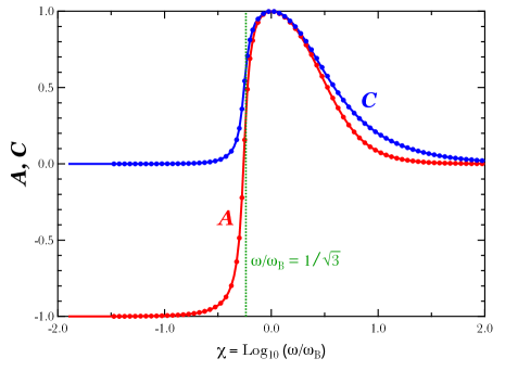
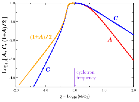
Figure 1: Left: Numerical solution of the master equations (points) at different logarithmic frequencies $\,\chi=\log_{10}(\omega/\omega_{\hbox{\fiverm B}})\,$ for $\,\cal A\,$ (anisotropy and linear polarization; red) and $\,\cal C\,$ (circular polarization; blue) together with the empirical approximations in Eqs. (35) and (LABEL:eq:calA_calClow_rat_fit) as the solid curves. The critical frequency $\,\omega=\omega_{\hbox{\fiverm B}}/\sqrt{3}\,$ where the cross sections for linear and circular polarizations are equal, is marked by the vertical green dashed line. Right: A logarithmic version of these solutions that helps visually illustrate the impressive agreement of the empirical approximations to the numerical solution data. While $\,\cal C\,$ is again represented by the blue curve and dots, and the red curve and dots constitute $\,\cal A\,$ when $\,\omega\geq\omega_{\hbox{\fiverm B}}\,$, the $\,\cal A\,$ information is presented instead as $\,(1+{\cal A})/2\,$ (orange dots and curve) below the cyclotron frequency (marked in mauve). Both the numerical solutions and the approximations accurately match the asymptotic results in Table 1 in the $\,\omega\ll\omega_{\hbox{\fiverm B}}\,$ and $\,\omega\gg\omega_{\hbox{\fiverm B}}\,$ domains.

For general utility of results, we opted not to generate extensive tables for display but rather to develop relatively compact analytic approximations that are easily encoded. This was an approach adopted in the Monte Carlo simulation analysis of Barchas et al. (2021), specifying empirical functions for $\,{\cal A}\,$ and $\,{\cal C}\,$ over the restricted frequency range $\,0.1\leq\omega/\omega_{\hbox{\fiverm B}}\leq 10\,$. The approximations identified in Eqs. (26) and (29) of Barchas et al. (2021) were of complex mathematical pathology that did not capture the polynomial character of the asymptotics listed in Table 1. Accordingly, they generally degraded in accuracy outside their frequency domain of development. Here, we deliver improved empirical approximations that are ratios of polynomials in the scaled frequency variable $\,x=\omega/\omega_{\hbox{\fiverm B}}\,$; we opt to use the $\,x\,$ variable mostly hereafter to render the ensuing mathematical expressions more compact. As in Barchas et al. (2021), it proved necessary to divide the frequency space into $\,x<1\,$ and $\,x\geq 1\,$ domains, and derive separate fits. A least squares fitting tool in Mathematica was employed, and the degrees of the polynomials in the numerator and the denominator were increased until an acceptable fit was achieved. The approximant was constrained by the $\,x\ll 1\,$ and $\,x\gg 1\,$ asymptotic forms in Table 1, as appropriate, and it was also constrained so that its first derivative in $\,x\,$ was zero at $\,x=1\,$, where both $\,{\cal A}\,$ and $\,{\cal C}\,$ achieve local maxima and values of unity. The resulting forms for the $\,x\geq 1\,$ range are

$${\cal A}(x)\;\approx\;\hbox{${{\displaystyle 17x^{4}+297x^{2}-30\vphantom{(}}\over{\displaystyle x^{2}(2x^{4}+43x^{2}+239)\vphantom{(}}}$}\quad,\quad{\cal C}(x)\;\approx\;\hbox{${{\displaystyle 2x^{2}+29x+15\vphantom{(}}\over{\displaystyle x^{3}+15x^{2}+30\vphantom{(}}}$}\quad,\qquad x\;=\;\hbox{${{\displaystyle\omega\vphantom{(}}\over{\displaystyle\omega_{\hbox{\fiverm B}}\vphantom{(}}}$}\;\geq\;1\quad.$$ (35)

The accuracies of these approximations are better than 0.8% for $\,\cal A\,$ and better than 0.9% for $\,\cal C\,$ at all frequencies.

For the $\,x=\omega/\omega_{\hbox{\fiverm B}}\leq 1\,$ domain, the empirical approximation fitting is somewhat more involved because of the functional dependences. The $\,{\cal A},{\cal C}\,$ variations in $\,x\,$ have a sharper transition between domains of shallow gradient, to steep gradient, to shallow gradient. This forces the inclusion of around double the number of terms in rational function approximations in order to deliver comparable precision. In addressing this $\,x\leq 1\,$ domain, it is simpler to work with $\,{\cal A}^{\prime}\equiv(1+{\cal A})/2\,$ as a proxy for $\,\cal A\,$ since it has a cleaner power-law character when $\,x\ll 1\,$: see Table 1. Furthermore, both $\,{\cal A}^{\prime}\,$ and $\,\cal C\,$ posses peak values of unity at the cyclotron frequency ($\,x=1\,$), and therefore have zero derivative in $\,x\,$ there. This character constrains the forms that the approximations can take. After considerable exploration, it was found that it was convenient to express the sub-cyclotronic rational function approximations using the proxy variable $\,\lambda(x)=1/x-x\,$ to force derivatives to zero at $\,x=1\,$ where $\,\lambda(x)=0\,$. For $\,x<1\,$, we have $\,\lambda(x)>0\,$. The empirical fitting functions then assumed the forms

$${\cal A}^{\prime} \equiv \hbox{${{\displaystyle 1+{\cal A}\vphantom{(}}\over{\displaystyle 2\vphantom{(}}}$}\;\approx\;\Biggl{\{}1+\sum_{j=1}^{4}n_{j}^{\cal A}\bigl{[}\lambda(x)\bigr{]}^{2j}\Biggr{\}}\Biggl{/}\Biggl{\{}1+\sum_{j=1}^{5}d_{j}^{\cal A}\bigl{[}\lambda(x)\bigr{]}^{2j}\Biggr{\}}$$

$${\cal C} \approx \hbox{${{\displaystyle 1\vphantom{(}}\over{\displaystyle 1+2\lambda^{3}(x)\vphantom{(}}}$}\Biggl{\{}1+\sum_{j=2}^{5}n_{j}^{\cal C}\bigl{[}\lambda(x)\bigr{]}^{2j}\Biggr{\}}\Biggl{/}\Biggl{\{}1+\sum_{j=1}^{5}d_{j}^{\cal C}\bigl{[}\lambda(x)\bigr{]}^{2j}\Biggr{\}}\quad\hbox{for}\quad\lambda(x)\;=\;\hbox{${{\displaystyle 1\vphantom{(}}\over{\displaystyle x\vphantom{(}}}$}-x\quad.$$

These forms automatically match $\,{\cal A}=1={\cal C}\,$ at $\,x=1\,$, and have zero derivatives there; they have Taylor series quadratic in $\,(x-1/x)\,$ about $\,x=1\,$. To match the $\,{\cal A}^{\prime}\approx x^{2}/4\,$ asymptotic limit for $\,x\ll 1\,$, we set $\,n_{4}^{\cal A}=d_{5}^{\cal A}/4\,$. For $\,\cal C\,$, when $\,x\ll 1\,$, the correct asymptotic behaviour is obtained if $\,n_{5}^{\cal C}=d_{5}^{\cal C}\,$. The least squares fitting protocol delivered numerical values for the numerator $\,n_{j}^{{\cal A},{\cal C}}\,$ and denominator $\,d_{j}^{{\cal A},{\cal C}}\,$ coefficients, with 8 free parameters. We judiciously approximated these by rational numbers without any significant degradation of precision, and in fact a slight improvement of such. The resulting coefficients are listed in Table 2. The empirical fits are accurate to better than $\,0.9\,$% for both $\,\cal A\,$ and $\,\cal C\,$ for all $\,x\leq 1\,$, and mostly better.

Table 2: Coefficients for $\,\cal A\,$ and $\,\cal C\,$ Empirical Fit Rational Functions

	$n_{1}^{{\cal A},{\cal C}}$	$n_{2}^{{\cal A},{\cal C}}$	$n_{3}^{{\cal A},{\cal C}}$	$n_{4}^{{\cal A},{\cal C}}$	$n_{5}^{{\cal A},{\cal C}}$	$d_{1}^{{\cal A},{\cal C}}$	$d_{2}^{{\cal A},{\cal C}}$	$d_{3}^{{\cal A},{\cal C}}$	$d_{4}^{{\cal A},{\cal C}}$	$d_{5}^{{\cal A},{\cal C}}$
${\cal A}^{\prime}$	$-\hbox{${{\displaystyle 15\vphantom{(}}\over{\displaystyle 19\vphantom{(}}}$}$	${{\displaystyle 9\vphantom{(}}\over{\displaystyle 32\vphantom{(}}}$	$-\hbox{${{\displaystyle 1\vphantom{(}}\over{\displaystyle 23\vphantom{(}}}$}$	${{\displaystyle 1\vphantom{(}}\over{\displaystyle 33\vphantom{(}}}$		$-\hbox{${{\displaystyle 7\vphantom{(}}\over{\displaystyle 10\vphantom{(}}}$}$	${{\displaystyle 1\vphantom{(}}\over{\displaystyle 5\vphantom{(}}}$	${{\displaystyle 1\vphantom{(}}\over{\displaystyle 5\vphantom{(}}}$	$-\hbox{${{\displaystyle 4\vphantom{(}}\over{\displaystyle 17\vphantom{(}}}$}$	$\hbox{${{\displaystyle 4\vphantom{(}}\over{\displaystyle 33\vphantom{(}}}$}=4n_{4}^{\cal A}$
${\cal C}$		${{\displaystyle 24\vphantom{(}}\over{\displaystyle 7\vphantom{(}}}$	$-\hbox{${{\displaystyle 21\vphantom{(}}\over{\displaystyle 16\vphantom{(}}}$}$	$-\hbox{${{\displaystyle 8\vphantom{(}}\over{\displaystyle 23\vphantom{(}}}$}$	${{\displaystyle 17\vphantom{(}}\over{\displaystyle 26\vphantom{(}}}$	$-\hbox{${{\displaystyle 1\vphantom{(}}\over{\displaystyle 4\vphantom{(}}}$}$	${{\displaystyle 16\vphantom{(}}\over{\displaystyle 19\vphantom{(}}}$	${{\displaystyle 2\vphantom{(}}\over{\displaystyle 7\vphantom{(}}}$	$-\hbox{${{\displaystyle 15\vphantom{(}}\over{\displaystyle 14\vphantom{(}}}$}$	$\hbox{${{\displaystyle 17\vphantom{(}}\over{\displaystyle 26\vphantom{(}}}$}=n_{5}^{\cal C}$

3.3 The Character of the Radiation Anisotropy and Polarization

.

The general character of the anisotropy and the polarization of the high opacity radiation configuration can be appraised by computing averages of the pertinent quantities over the pre-scattering photon angles. To this end, we now form integrals of $\,\hat{Q}\,$, $\,\hat{V}\,$ in Eq. (24) over $\,\mu\,$ on the interval $\,0\leq\mu\leq 1\,$, which serve as average measures. Note that other averages are possible, for example forming integrals over $\,Q\,$ and $\,V\,$ divided by that for $\,I\,$; adopting such does not materially alter the conclusions we draw just below. The averages resulting from our protocol are

$$\bigl{\langle}\hat{Q}\bigr{\rangle}\;=\;1-\bigl{(}1+{\cal A}\bigr{)}u\bigl{(}{\cal A}\bigr{)}\quad,\quad\bigl{\langle}\hat{V}\bigr{\rangle}\;=\;\hbox{${{\displaystyle{\cal C}\,\log_{e}\bigl{(}1+{\cal A}\bigr{)}\vphantom{(}}\over{\displaystyle{\cal A}\vphantom{(}}}$}\;\quad\hbox{for}\quad\;u(z)\;=\;\begin{cases}\hbox{${{\displaystyle\arctan(\sqrt{z})\vphantom{(}}\over{\displaystyle\sqrt{z}\vphantom{(}}}$}\quad,&\text{if}\;\;z>0\;\;,\\ \hbox{${{\displaystyle 1\vphantom{(}}\over{\displaystyle 2\sqrt{|z|}\vphantom{(}}}$}\log_{e}\hbox{${{\displaystyle 1+\sqrt{|z|}\vphantom{(}}\over{\displaystyle 1-\sqrt{|z|}\vphantom{(}}}$}\quad,&\text{if}\;\;z<0\;\;.\\ \end{cases}$$ (37)

Similar forms can quickly be obtained for the accompanying linear polarization quantities $\,\hat{I}_{\parallel}\,$ and $\,\hat{I}_{\perp}\,$:

$$\bigl{\langle}\hat{I}_{\parallel}\bigr{\rangle}\;=\;1-\bigl{(}1+{\cal A}\bigr{)}\hbox{${{\displaystyle u\bigl{(}{\cal A}\bigr{)}\vphantom{(}}\over{\displaystyle 2\vphantom{(}}}$}\quad,\quad\bigl{\langle}\hat{I}_{\perp}\bigr{\rangle}\;=\;\bigl{(}1+{\cal A}\bigr{)}\hbox{${{\displaystyle u\bigl{(}{\cal A}\bigr{)}\vphantom{(}}\over{\displaystyle 2\vphantom{(}}}$}\;=\;1-\bigl{\langle}\hat{I}_{\parallel}\bigr{\rangle}\quad.$$ (38)

These forms are now purely functions of the frequency ratio, $\,x=\omega/\omega_{\hbox{\fiverm B}}\,$, and are plotted in Fig. 2, left, to illustrate the dependence on $\,x\,$. A number of features are apparent, all being consequences of the character of the scattering cross section that is presented in Appendix B of Barchas et al. (2021). In the low frequency domain, $\,\omega\ll\omega_{\hbox{\fiverm B}}\,$, there is a clear dominance of the $\,\parallel\,$ polarization mode, with $\,\bigl{\langle}\hat{I}_{\parallel}\bigr{\rangle}\to 1\,$ corresponding to $\,Q\to 1\,$. There are rapid variations in all these average polarization quantities in the neighborhood of $\,\omega/\omega_{\hbox{\fiverm B}}=1/\sqrt{3}\,$ as the competition between circular and linear polarization in the scattering cross section becomes significant. Circular polarization peaks at $\,\omega=\omega_{\hbox{\fiverm B}}\,$, with $\,\bigl{\langle}\hat{V}\bigr{\rangle}=\log_{e}2\approx 0.69\,$, accompanied by a minimum of $\,\bigl{\langle}\hat{Q}\bigr{\rangle}=1-\pi/2\approx-0.57\,$. Around the cyclotron frequency and above it, the $\,\perp\,$ mode is dominant in the photon configuration. Finally, in the non-magnetic regime, $\,\omega\gg\omega_{\hbox{\fiverm B}}\,$, the high opacity configuration is essentially unpolarized, with $\,\bigl{\langle}\hat{I}_{\parallel}\bigr{\rangle}\approx\bigl{\langle}\hat{I}_{\perp}\bigr{\rangle}\approx 1/2\,$.

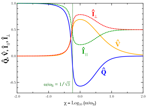
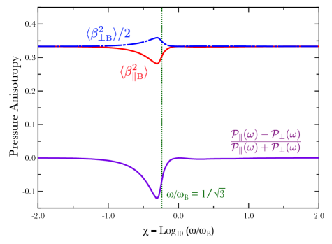
Figure 2: Left: Angle-averaged polarization measures $\,\bigl{\langle}\hat{Q}\bigr{\rangle}\,$ and $\,\bigl{\langle}\hat{V}\bigr{\rangle}\,$, as defined in Eq. (37), and $\,\bigl{\langle}\hat{I}_{\parallel}\bigr{\rangle}\,$ and $\,\bigl{\langle}\hat{I}_{\perp}\bigr{\rangle}\,$, as given in Eq. (38), as functions of the logarithm of the dimensionless photon frequency $\,\omega/\omega_{\hbox{\fiverm B}}\,$. In the non-magnetic domain, $\,\omega\gg\omega_{\hbox{\fiverm B}}\,$, they evince an unpolarized configuration. In the highly-magnetic regime, $\,\omega\ll\omega_{\hbox{\fiverm B}}\,$, dominance of the $\,\parallel\,$ polarization mode ($\,Q\to 1\,$) is clear. All quantities exhibit extrema at the cyclotron frequency, and vary rapidly around $\,\omega/\omega_{\hbox{\fiverm B}}=1/\sqrt{3}\,$. Right: Radiation anisotropy measures $\,\langle\beta^{2}_{\parallel\hbox{\sixrm B}}\rangle\,$, as defined in Eq. (40), and its counterpart $\,\langle\beta^{2}_{\perp\hbox{\sixrm B}}\rangle/2\,$. These two are approximately equal to $\,1/3\,$ when $\,\omega\mathrel{\mathchoice{\lower 2.0pt\vbox{\halign{$\m@th\displaystyle\hfil#\hfil$\cr>\crcr\sim\crcr}}}{\lower 2.0pt\vbox{\halign{$\m@th\textstyle\hfil#\hfil$\cr>\crcr\sim\crcr}}}{\lower 2.0pt\vbox{\halign{$\m@th\scriptstyle\hfil#\hfil$\cr>\crcr\sim\crcr}}}{\lower 2.0pt\vbox{\halign{$\m@th\scriptscriptstyle\hfil#\hfil$\cr>\crcr\sim\crcr}}}}\omega_{\hbox{\fiverm B}}\,$ and also when $\,\omega\ll\omega_{\hbox{\fiverm B}}\,$, when approximate isotropy exists; only when $\,\omega/\omega_{\hbox{\fiverm B}}\sim 1/\sqrt{3}\,$ is there significant radiation anisotropy. Also depicted is the pressure anisotropy function given in Eq. (41). A modest dominance of pressure perpendicular to $\,\boldsymbol{B}\,$ at sub-cyclotronic $\,\omega/\omega_{\hbox{\fiverm B}}\sim 1/\sqrt{3}\,$ frequencies is evident.

An additional piece of information concerns the anisotropy of the radiation field. By inspection of Eq. (19), the angular intensity is proportional to $\,(1+{\cal A}\mu^{2})/\sigma(\omega,\,\mu)\,$, where $\,\sigma(\omega,\,\mu)\,$ is expressed in Eq. (26). This connection with the $\,\Lambda_{I}(\mu)\,$ redistribution anisotropy function is discussed at length in Section 5.3 of Barchas et al. (2021). There are two anisotropy measures that connect to the pressure that the radiation field can exert on a strongly-magnetized electron gas along the direction of $\,\boldsymbol{B}\,$, and perpendicular to it. The pertinence of radiation pressure is discussed briefly in Sec. 4. The pressure tensor consists of summations over $\,p^{i}v^{j}\,$ products from components of momentum ($\,p^{i}\,$) in the $\,i^{th}\,$ coordinate direction, and velocity ($\,v^{j}\,$) in the $\,j^{th}\,$ direction:

$${\cal P}_{ij}\;=\;\int n_{\gamma}\bigl{(}\mathbf{p}\bigr{)}\,p^{i}v^{j}\,d^{3}p\quad,$$ (39)

where $\,n_{\gamma}\bigl{(}\mathbf{p}\bigr{)}\propto(1+{\cal A}\mu^{2})/\sigma(\omega,\,\mu)\,$ is the number density of photons per momentum interval $\,\mathbf{dp}\,$ that can be obtained directly from the angle-dependent intensity. Clearly, $\,{\cal P}_{ij}\,$ constitutes the purely spatial portion of the energy-momentum tensor (Weinberg, 1972) in the special case where there are no bulk relativistic motions. Considering only diagonal elements, the two pertinent radiation anisotropy measures can be distilled into averages of the velocity components (in units of $\,c\,$) parallel to ($\,\beta^{2}_{\parallel\hbox{\sixrm B}}=\mu^{2}\,$) and orthogonal ($\,\beta^{2}_{\perp\hbox{\sixrm B}}=1-\mu^{2}\,$) to $\,\boldsymbol{B}\,$, and are obviously not independent quantities. The anisotropic pressure tensor diagonal elements are thus $\,{\cal P}_{\parallel}(\omega)\propto\langle\beta^{2}_{\parallel\hbox{\sixrm B}}\rangle\,$ along $\,\boldsymbol{B}\,$, and $\,{\cal P}_{\perp}(\omega)\propto\langle\beta^{2}_{\perp\hbox{\sixrm B}}\rangle/2=\bigl{[}1-\langle\beta^{2}_{\parallel\hbox{\sixrm B}}\rangle\bigr{]}/2\,$ in the plane that is orthogonal to the field, noting that the coefficients of proportionality in these relations are identical. If one scales the cross section according to $\,\sigma(\omega,\,\mu)/\sigma_{\hbox{\sixrm T}}=\overline{\sigma}(\omega,\,\mu)/(1+{\cal A}\mu^{2})\,$, so that $\,\overline{\sigma}(\omega,\,\mu)\,$ is a dimensionless quadratic function of $\,\mu^{2}\,$, one can form the average

$$\langle\beta^{2}_{\parallel\hbox{\sixrm B}}\rangle\;=\;\int_{0}^{1}\hbox{${{\displaystyle\mu^{2}\bigl{(}1+{\cal A}\mu^{2}\bigr{)}^{2}\vphantom{(}}\over{\displaystyle\overline{\sigma}(\omega,\,\mu)\vphantom{(}}}$}\,d\mu\Biggl{/}\int_{0}^{1}\hbox{${{\displaystyle\bigl{(}1+{\cal A}\mu^{2}\bigr{)}^{2}\vphantom{(}}\over{\displaystyle\overline{\sigma}(\omega,\,\mu)\vphantom{(}}}$}\,d\mu\quad.$$ (40)

The pressure anisotropy at a single photon frequency is then

$$\hbox{${{\displaystyle{\cal P}_{\parallel}(\omega)-{\cal P}_{\perp}(\omega)\vphantom{(}}\over{\displaystyle{\cal P}_{\parallel}(\omega)+{\cal P}_{\perp}(\omega)\vphantom{(}}}$}\;=\;\hbox{${{\displaystyle 3\langle\beta^{2}_{\parallel\hbox{\sixrm B}}\rangle-1\vphantom{(}}\over{\displaystyle\langle\beta^{2}_{\parallel\hbox{\sixrm B}}\rangle+1\vphantom{(}}}$}\quad.$$ (41)

This pressure anisotropy function of $\,\omega/\omega_{\hbox{\fiverm B}}\,$ is plotted along with $\,\langle\beta^{2}_{\parallel\hbox{\sixrm B}}\rangle\,$ and $\,\langle\beta^{2}_{\perp\hbox{\sixrm B}}\rangle/2\,$ in the right panel of Fig. 2. At $\,\omega\ll\omega_{\hbox{\fiverm B}}\,$ frequencies, and also in the non-magnetic $\,\omega/\omega_{\hbox{\fiverm B}}\gg 1\,$ domain, $\,\langle\beta^{2}_{\perp\hbox{\sixrm B}}\rangle/2\approx\langle\beta^{2}_{\parallel\hbox{\sixrm B}}\rangle\approx 1/3\,$ and pressure isotropy prevails: $\,{\cal P}_{\perp}(\omega)\approx{\cal P}_{\parallel}(\omega)\,$. The same circumstance arises in the cyclotron resonance, $\,\omega\approx\omega_{\hbox{\fiverm B}}\,$. For all three of these domains, the cross section and $\,\cal A\,$ values in Table 1 can be used to show that $\,\langle\beta^{2}_{\parallel\hbox{\sixrm B}}\rangle\approx 1/3\,$. In contrast, when $\,\omega/\omega_{\hbox{\fiverm B}}\sim 1/\sqrt{3}\,$, then $\,\langle\beta^{2}_{\perp\hbox{\sixrm B}}\rangle/2>1/3>\langle\beta^{2}_{\parallel\hbox{\sixrm B}}\rangle\,$, and more pressure appears at large angles to $\,\boldsymbol{B}\,$ than is generally in the direction of the field. Yet, the pressure anisotropy is still only at the $\,\sim 10\,$% level. These determinations follow from the prevailing general isotropy of the radiation field that is evident in Fig. 8 of Barchas et al. (2021), with the largest anisotropy being for $\,\omega/\omega_{\hbox{\fiverm B}}\sim 1/\sqrt{3}\,$. To generate the complete pressure information, these results would need to be integrated over the photon spectrum pertinent to a particular astrophysical setting; this task is the purview of other work.

The numerical solution for the coefficients $\,\cal A\,$ and $\,\cal C\,$ also enables the complete specification of the polarized total cross section $\,\sigma(\omega,\,\mu)\,$ in Eq. (26) appropriate for the high opacity domain. Its behavior is plotted as a function of $\,\mu\,$ for different frequencies in Fig. 3, wherein the curves are normalized to unit area in the $\,\mu\,$ variable. Specifically, the cross section can be averaged over all incoming photon angles thus:

$$\sigma(\omega)\;\equiv\;\bigl{\langle}\sigma(\omega,\,\mu)\bigr{\rangle}\;=\;\int_{0}^{1}\sigma(\omega,\,\mu)\,d\mu\quad,$$ (42)

which, for $\,u(z)\,$ as defined in Eq. (37), yields an evaluation

$$\sigma(\omega)\;=\;\sigma_{\hbox{\sixrm T}}\biggl{\{}\Sigma_{\hbox{\sixrm B}}+\hbox{${{\displaystyle 1-\Sigma_{\hbox{\sixrm B}}\vphantom{(}}\over{\displaystyle 2{\cal A}\vphantom{(}}}$}\left[1+\hbox{${{\displaystyle 7{\cal A}\vphantom{(}}\over{\displaystyle 3\vphantom{(}}}$}-\bigl{(}1+{\cal A}\bigr{)}^{2}u\bigl{(}{\cal A}\bigr{)}\right]+\hbox{${{\displaystyle 2{\cal C}\Delta_{\hbox{\sixrm B}}\vphantom{(}}\over{\displaystyle{\cal A}\vphantom{(}}}$}\,\Bigl{[}1-u\bigl{(}{\cal A}\bigr{)}\Bigr{]}\biggr{\}}.\quad.$$ (43)

This average is employed to normalize the curves in Fig. 3 in presenting the variations of $\,\sigma(\omega,\,\mu)/\bigl{\langle}\sigma(\omega,\,\mu)\bigr{\rangle}\,$. At $\,\omega\gg\omega_{\hbox{\fiverm B}}\,$ frequencies, $\,\sigma(\omega,\,\mu)\approx\sigma_{\hbox{\sixrm T}}\,$ and the non-magnetic Thomson domain is realized. As $\,\omega\,$ drops towards the cyclotron frequency, the cross section preferentially favors scatterings of photons directed more along the field direction, a profound influence on radiative transfer at high opacities. This behavior continues smoothly through and below the cyclotron frequency as the depiction moves from the right to the left panels. Once the frequency drops below the bifurcation value, $\,\omega_{\hbox{\fiverm B}}/\sqrt{3}\,$, the influence of circular polarizations diminishes and the character transitions to describe a $\,\omega\ll\omega_{\hbox{\fiverm B}}\,$ domain where scatterings of photons moving approximately perpendicular to $\,\boldsymbol{B}\,$ are more prevalent than those for photons closer to the field direction. Finally, note that this cross section behavior contributes to the angular dependence of the intensity $\,I(\mu)\propto(1+{\cal A}\mu^{2})/\sigma(\omega,\,\mu)\,$; examples of such intensity distributions are given in Fig. 8 of Barchas et al. (2021).

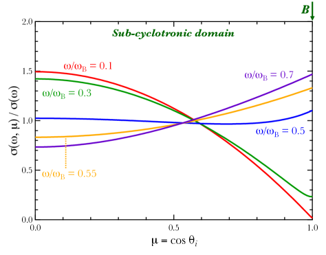
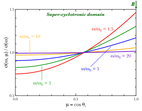
Figure 3: The polarized, magnetic Thomson cross section $\,\sigma(\omega,\,\mu)\,$ at high opacities, i.e. that in Eq. (26), as a function of the angle cosine $\,\mu=\cos\theta_{i}\,$ of the incoming photon to the magnetic field direction $\,\boldsymbol{B}\,$ that is indicated at the upper right of each panel. The left panel corresponds to the $\,\omega<\omega_{\hbox{\fiverm B}}\,$ sub-cyclotron domain, and the right panel is for cases of incoming photons above the cyclotron energy. The polarization configuration is from the empirical formulae in Eqs. (35) and (LABEL:eq:calA_calClow_rat_fit), and the cross sections are scaled in units of the total (polarized and magnetic) cross section $\,\sigma(\omega)\,$. When $\,\omega\gg\omega_{\hbox{\fiverm B}}\,$, the cross section becomes independent of $\,\mu\,$ and $\,\sigma(\omega,\,\mu)\to\sigma_{\hbox{\sixrm T}}\,$ as well as $\,\sigma(\omega)\to\sigma_{\hbox{\sixrm T}}\,$, the familiar non-magnetic regime. For the $\,\omega\ll\omega_{\hbox{\fiverm B}}\,$ domain, the $\,\omega/\omega_{\hbox{\fiverm B}}=0.1\,$ curve closely approximates the $\,3(1-\mu^{2})/2\,$ asymptotic result. See Table. 1.

4 Discussion

A principal motivation for our derivation of precision numerical solutions to the high opacity domain of the polarized Thomson scattering transport equations in cold, magnetized plasmas is that it facilitates improved efficiency of transport simulations. This is demonstrated in Fig. 2 of Hu et al. (2022), wherein intensities and Stokes parameter solutions for the Monte Carlo simulation MAGTHOMSCATT of radiation transfer in slabs of fixed Thomson optical depths are compared for two protocols of photon injection at the base of the slab. The first was a simple injection of isotropic and unpolarized photons (designated IU injection) at the base of the simulation slab, identical for all $\,\omega/\omega_{\hbox{\fiverm B}}\,$, with the ultimate observer signal being recorded for those photons that exit the slab at its opposite, upper planar surface. The alternative was for a frequency-dependent anisotropic and polarized (AP) photon injection that employed the Stokes parameter and anisotropy information encapsulated in Eq. (24), i.e. pertaining to the high opacity configuration. Hu et al. (2022) performed a limited exploration of the relative efficacy of the two injection protocols, finding that the AP choice generally required slightly or somewhat smaller effective optical depths $\,\tau_{\rm eff}\,$ to realize convergent solutions that did not vary when the slab thickness was further increased. The definition of $\,\tau_{\rm eff}\,$ is given in Eq. (5) of Hu et al. (2022):

$$\tau_{{\hbox{\sixrm eff}}}\;=\;n_{e}h\,\sigma_{\rm up}(\theta_{i}\;=\;\theta_{\hbox{\fiverm B}})\;=\;\hbox{${{\displaystyle\tau_{\hbox{\sixrm T}}\vphantom{(}}\over{\displaystyle 2\vphantom{(}}}$}\Bigl{\{}\sin^{2}\theta_{\hbox{\fiverm B}}+\Sigma_{\hbox{\sixrm B}}(\omega)\left[1+\cos^{2}\theta_{\hbox{\fiverm B}}\right]\Bigr{\}}\quad.$$ (44)

It is posited based on the unpolarized Thomson cross section $\,\sigma_{\rm up}\,$ evaluated for pre-scattering photon directions along the local slab zenith, and therefore at incidence angle $\,\theta_{i}=\theta_{\hbox{\fiverm B}}\,$ to the field $\,\boldsymbol{B}\,$. Clearly, while it couples with the Thomson value $\,\tau_{\hbox{\sixrm T}}=n_{e}\sigma_{\hbox{\sixrm T}}h\,$ for slabs of thickness $\,h\,$ and electron number density $\,n_{e}\,$, it depends significantly on the photon frequency and the orientation of the field direction to the slab’s zenith/normal.

Here, we deliver a more detailed and precise assessment of how the AP injection protocol compares in efficiency with the IU one in MAGTHOMSCATT. For this exploration, the empirical forms for $\,\cal A\,$ and $\,\cal C\,$ in Eqs. (35) and (LABEL:eq:calA_calClow_rat_fit) were encoded in the simulation so as to test their usefulness. Another upgrade was to render MAGTHOMSCATT in fully parallelized form so that it was run on Rice University’s NOTS cluster. This development opened up access to high statistics runs for $\,\omega/\omega_{\hbox{\fiverm B}}\leq 0.1\,$ that are generally slower due to the wide disparity of the cross sections over the full range of photon polarizations and propagation directions. $\,\tau_{\rm eff}\,$ values (denoted $\,\tau_{\rm eff,AP}\,$ and $\,\tau_{\rm eff,IU}\,$) and associated run times ($\,t_{\hbox{\sixrm AP}}\,$ and $\,t_{\hbox{\sixrm IU}}\,$) required to deliver convergent simulations were obtained for a variety of frequency ratios $\,0.01\leq\omega/\omega_{\hbox{\fiverm B}}\leq 10\,$ spanning the cyclotron resonance region. Results are presented in Table 3, where the run time ratios $\,t_{\hbox{\sixrm IU}}/t_{\hbox{\sixrm AP}}\,$ are listed since the actual run times depend on the scale and configuration of any machine cluster. Note that all simulations were performed in exactly the same run protocol (and $\,10^{6}\,$ photons) so that relative simulation times could be accurately calibrated. More details on the run times across the spectrum of atmosphere parameters $\,\theta_{\hbox{\fiverm B}}\,$ and $\,\omega/\omega_{\hbox{\fiverm B}}\,$ will be provided in Dinh Thi et al. (in preparation). The definition of convergence was that the output from the upper slab surface of all of the relevant Stokes parameter information ($\,I,Q,V\,$) does not change appreciably when the effective slab optical depth $\,\tau_{\rm eff}\,$ was increased above the nominal values listed here in Table 3. This information consisted primarily of the zenith angle distributions like those presented in Figure 2 of Hu et al. (2022). Select zenith angles $\,\theta_{\hbox{\fiverm B}}\,$ for the magnetic field were sampled, encompassing magnetic polar, equatorial and mid-latitude locales of the Thomson scattering atmospheric slab on a neutron star surface threaded by a magnetic dipole.

Table 3: Effective optical depths $\,\tau_{\rm eff,AP}\,$ and $\,\tau_{\rm eff,IU}\,$ and run time ratios $\,t_{\hbox{\sixrm IU}}/t_{\hbox{\sixrm AP}}\,$ for IU and AP injection protocols in MAGTHOMSCATT

	$\omega/\omega_{\hbox{\fiverm B}}$	10	3	0.99	0.3	0.1	0.03	0.01
	$\tau_{\rm eff,IU}$	6	6	9	6	8	8	10
$\theta_{\hbox{\fiverm B}}=0^{\circ}$	$\tau_{\rm eff,AP}$	6	6	6	6	6	6	6
	$t_{\hbox{\sixrm IU}}/t_{\hbox{\sixrm AP}}\vskip 1.5pt$	1	0.91	1.18	0.77	1.08	1.50	2.41
	$\tau_{\rm eff,IU}$	6	8	10	20	50	400	$>$ 800
$\theta_{\hbox{\fiverm B}}=30^{\circ}$	$\tau_{\rm eff,AP}$	6	6	6	15	30	150	200
	$t_{\hbox{\sixrm IU}}/t_{\hbox{\sixrm AP}}\vskip 1.5pt$	0.96	1.55	1.04	1.56	1.93	5.76	$>$ 5.69
	$\tau_{\rm eff,IU}$	10	8	20	30	100	600	$>$ 800
$\theta_{\hbox{\fiverm B}}=60^{\circ}$	$\tau_{\rm eff,AP}$	8	6	6	20	30	200	200
	$t_{\hbox{\sixrm IU}}/t_{\hbox{\sixrm AP}}\vskip 1.5pt$	1.30	1.31	3.68	1.24	4.32	5.43	$>$ 6.77
	$\tau_{\rm eff,IU}$	6	8	20	20	200	1000	$>$ 1600
$\theta_{\hbox{\fiverm B}}=90^{\circ}$	$\tau_{\rm eff,AP}$	6	6	6	6	10	10	10
	$t_{\hbox{\sixrm IU}}/t_{\hbox{\sixrm AP}}\vskip 1.5pt$	0.77	1.16	4.58	3.32	112	2183	$>$ 3469

The comparison of minimum slab effective optical depths $\,\tau_{\rm eff,AP}\,$ and $\,\tau_{\rm eff,IU}\,$ in Table 3, which are discretized to integer values, clearly indicates that higher $\,\tau_{\rm eff}\,$ are required for IU injections around or below the cyclotron frequency. This is a consequence of the AP injection more closely resembling the photon anisotropy and polarization configuration at the same distance from the surface for $\,\tau_{\rm eff}\to\infty\,$ atmospheres. In the super-cyclotronic domain, the injection protocol does not matter, generating similar $\,\tau_{\rm eff}\,$ and run times. In fact, above around $\,\omega/\omega_{\hbox{\fiverm B}}\sim 1/\sqrt{3}\,$, the MAGTHOMSCATT code can be run with either injection choice with similar efficiency. In contrast, when $\,\omega/\omega_{\hbox{\fiverm B}}\,$ drops to around 0.1 or lower, the AP injection protocol quickly becomes more efficient and therefore preferred. This is particularly so for mid-latitude and equatorial locales ($\,\theta_{\hbox{\fiverm B}}\mathrel{\mathchoice{\lower 2.0pt\vbox{\halign{$\m@th\displaystyle\hfil#\hfil$\cr>\crcr\sim\crcr}}}{\lower 2.0pt\vbox{\halign{$\m@th\textstyle\hfil#\hfil$\cr>\crcr\sim\crcr}}}{\lower 2.0pt\vbox{\halign{$\m@th\scriptstyle\hfil#\hfil$\cr>\crcr\sim\crcr}}}{\lower 2.0pt\vbox{\halign{$\m@th\scriptscriptstyle\hfil#\hfil$\cr>\crcr\sim\crcr}}}}30^{\circ}\,$), for which the AP choice leads to a much lower convergence $\,\tau_{\rm eff}\,$ and much shorter run times than IU does. Notably, in a number of cases, the IU runs did not realize convergence for $\,\omega/\omega_{\hbox{\fiverm B}}=0.01\,$ and locales away from the magnetic pole with simulation run times inferior to 24 hours on the cluster. Accordingly, the developments of precision high opacity AP configurations that are delivered in this paper are particularly helpful for the simulation of magnetar atmospheres, which generally sample $\,\omega/\omega_{\hbox{\fiverm B}}<0.01\,$ domains. Again, the reason for this originates in the wide disparity of the scattering cross sections that are sampled over the full range of photon polarizations and propagation directions relative to $\,\boldsymbol{B}\,$.

The high opacity radiative transfer analysis presented herein is useful for radiation dynamics considerations in various neutron star settings. The anisotropy elements addressed in Sec. 3.3 enable the specification of various radiation pressure tensor components in an anisotropic, magnetized plasma. Knowledge of this pressure tensor is important for accurate modeling of super-Eddington environments. The most notable of these are the common bursts and rare giant flares of magnetars, both of which have luminosities well above the Eddington limit, and via simple energetics considerations must be highly opaque to Thomson scattering (e.g., Lin et al., 2012; Taverna & Turolla, 2017). Consequently, the intense radiation pressure in both these types of magnetar transients must drive the emitting plasma to move relativistically. The speeds of the motions are governed by dynamics, and will critically influence the spectrum of the radiation we detect (Lin et al., 2012; Roberts et al., 2021), and likely its polarization also, thereby providing a science agenda for future hard X-ray polarimeters. Accordingly, a deep understanding of radiation pressure in the burst/flare emission regions at various magnetospheric locales with different field strengths and plasma temperatures is required to forge detailed models of these short-lived events. Such understanding is enabled by the specification of the high opacity forms for the scaled Stokes parameters in Eq. (24) and resultant cross section in Eq. (43) with great precision at a wide range of photon and electron cyclotron frequencies. These forms can be readily employed in both cold and warm plasma settings in neutron star magnetospheres.

The analysis can also be applied to the hydrostatics of accretion columns in high mass X-ray binaries, where near-Eddington luminosities suggest an active emission region that resides in the polar column at a location offset from the stellar surface due to intense radiation pressure (e.g. Becker, 1998; Schwarm et al., 2017), the historical “fan-beam” scenario. The forms in Eq. (24) in combination with the anisotropic cross section in Eq. (43) can assist in improving the determination of the stand-off accretion shock altitude that was a focus in Becker (1998). This in turn informs estimates of the neutron star surface field that couple to the accretion shock fields obtained from hard X-ray cyclotron absorption lines in these systems. While the MAGTHOMSCATT simulation was envisaged and devised for neutron star surface applications, it is readily adaptable to high $\,\tau_{\hbox{\sixrm T}}\,$ magnetospheric problems, both for X-ray binaries and for magnetars. The caveat with this is that ideally the cross section should be upgraded to the full QED magnetic Compton form (e.g., Daugherty & Harding, 1986; Gonthier et al., 2014; Mushtukov et al., 2016), a somewhat formidable task given the mathematical complexity associated with the many cyclotron harmonics. Efforts by our broader group to deliver such QED Compton cross section forms that are convenient for radiative transfer simulations of magnetar emission zones are continuing (Gonthier et al., in preparation). At the generally lower fields present in X-ray binary accretion columns, QED cross sections for radiative transfer near the cyclotron fundamental and low harmonics have been implemented in the simulations of Araya & Harding (1999) and Schwarm et al. (2017) in the quest for precision studies of cyclotron line formation.

5 Conclusion

For cold, magnetized plasmas, this paper has presented a radiative transfer equation analysis of the asymptotic configuration of radiation anisotropy and polarization in the limit of high Thomson scattering opacity, $\,\tau_{\hbox{\sixrm T}}=n_{e}\sigma_{\hbox{\sixrm T}}h\gg 1\,$. The focus was on the influence of a strong magnetic field on the equilibrium photon population via the determination of Stokes parameters at different frequencies $\,\omega\,$ relative to the cyclotron frequency $\,\omega_{\hbox{\fiverm B}}\,$. The methodology distilled a phase matrix formalism down to two integral equations capturing information on the two eigenmodes of radiation propagation in the plasma. These master equations constitute a Neumann problem that was solved numerically, additionally identifying useful analytic solutions in the highly-magnetic, $\,\omega\ll\omega_{\hbox{\fiverm B}}\,$, and essentially non-magnetic, $\,\omega\gg\omega_{\hbox{\fiverm B}}\,$, domains. Based on these solutions and asymptotic analytic forms, empirical approximations for the two key parametric functions $\,{\cal A}(\omega)\,$ (representing anisotropy) and $\,{\cal C}(\omega)\,$ (representing circularity) were delivered. These were then employed to illustrate how the magnetic Thomson Monte Carlo transport simulation MAGTHOMSCATT was made more efficient with the use of the high opacity anisotropy and polarization (AP) configuration in the photon injection protocol at the bottom of an atmospheric slab. For different surface locales, Table 3 lists the values of the effective slab optical depth parameter $\,\tau_{{\hbox{\sixrm eff}}}\,$ that guaranteed convergent determinations of the emergent anisotropy and polarization for photons exiting the top of the slab. Code speed-up relative to isotropic/unpolarized injection protocols was also listed in Table 3, and it was greatest at $\,\omega\ll\omega_{\hbox{\fiverm B}}\,$ frequencies and for magnetic fields lying closer to the atmospheric horizon (i.e., surface equatorial zones), a case germane also to the modeling of magnetar bursts in their magnetospheres. The anisotropic pressure determinations for the high opacity photon configuration will also prove useful in modeling the hydrostatics and dynamics of near-Eddington and super-Eddington neutron star environments such as accretion columns in X-ray binaries, and bursts and giant flares in magnetars.

Appendix A

Phase Matrix Elements

Here we list the nine phase matrix elements that do not integrate to zero in Eq. (10) on the azimuthal interval $\,0\leq\phi_{fi}\leq 2\pi\,$. The other seven, being odd functions of $\,\phi_{fi}\,$ on $\,[0,\,2\pi]\,$, and therefore not germane to the radiative transfer developments of this paper, can be found in Eq. (2) of Whitney (1991) and pages 42-43 of Barchas (2017). For $\,x=\omega/\omega_{\hbox{\fiverm B}}\,$, using the scaled form $\,\hat{P}_{if}={P}_{if}\,\sigma(\omega,\,\mu_{i})/r_{0}^{2}\,$ identified in Eq. (5), these elements are

$$\hat{P}_{11} = \sin^{2}\theta_{i}\sin^{2}\theta_{f}+\hbox{${{\displaystyle x^{2}\vphantom{(}}\over{\displaystyle(x^{2}-1)^{2}\vphantom{(}}}$}\,\cos^{2}\theta_{i}\cos^{2}\theta_{f}\Bigl{[}x^{2}\cos^{2}\phi_{fi}+\sin^{2}\phi_{fi}\Bigr{]}+\hbox{${{\displaystyle x^{2}\vphantom{(}}\over{\displaystyle 2(x^{2}-1)\vphantom{(}}}$}\sin 2\theta_{i}\sin 2\theta_{f}\,\cos\phi_{fi}$$

$$\hat{P}_{12} = \hbox{${{\displaystyle x^{2}\vphantom{(}}\over{\displaystyle(x^{2}-1)^{2}\vphantom{(}}}$}\,\cos^{2}\theta_{f}\Bigl{[}\cos^{2}\phi_{fi}+x^{2}\sin^{2}\phi_{fi}\Bigr{]}$$

$$\hat{P}_{14} = \hbox{${{\displaystyle x^{3}\vphantom{(}}\over{\displaystyle(x^{2}-1)^{2}\vphantom{(}}}$}\cos\theta_{i}\cos^{2}\theta_{f}+\hbox{${{\displaystyle x\vphantom{(}}\over{\displaystyle 2(x^{2}-1)\vphantom{(}}}$}\,\sin\theta_{i}\sin 2\theta_{f}\,\cos\phi_{fi}$$

$$\hat{P}_{21} = \hbox{${{\displaystyle x^{2}\vphantom{(}}\over{\displaystyle(x^{2}-1)^{2}\vphantom{(}}}$}\,\cos^{2}\theta_{i}\Bigl{[}\cos^{2}\phi_{fi}+x^{2}\sin^{2}\phi_{fi}\Bigr{]}$$

$$\hat{P}_{22} = \hbox{${{\displaystyle x^{2}\vphantom{(}}\over{\displaystyle(x^{2}-1)^{2}\vphantom{(}}}$}\,\Bigl{[}x^{2}\cos^{2}\phi_{fi}+\sin^{2}\phi_{fi}\Bigr{]}$$ (1)

$$\hat{P}_{24} = \hbox{${{\displaystyle x^{3}\vphantom{(}}\over{\displaystyle(x^{2}-1)^{2}\vphantom{(}}}$}\,\cos\theta_{i}$$

$$\hat{P}_{41} = \hbox{${{\displaystyle 2x^{3}\vphantom{(}}\over{\displaystyle(x^{2}-1)^{2}\vphantom{(}}}$}\,\cos^{2}\theta_{i}\cos\theta_{f}+\hbox{${{\displaystyle x\vphantom{(}}\over{\displaystyle x^{2}-1\vphantom{(}}}$}\sin 2\theta_{i}\sin\theta_{f}\,\cos\phi_{fi}$$

$$\hat{P}_{42} = \hbox{${{\displaystyle 2x^{3}\vphantom{(}}\over{\displaystyle(x^{2}-1)^{2}\vphantom{(}}}$}\,\cos\theta_{f}$$

$$\hat{P}_{44} = \hbox{${{\displaystyle x^{2}(x^{2}+1)\vphantom{(}}\over{\displaystyle(x^{2}-1)^{2}\vphantom{(}}}$}\cos\theta_{i}\cos\theta_{f}+\hbox{${{\displaystyle x^{2}\vphantom{(}}\over{\displaystyle x^{2}-1\vphantom{(}}}$}\,\sin\theta_{i}\sin\theta_{f}\,\cos\phi_{fi}\quad.$$

These are the forms that are inserted into the re-distribution function integral in Eq. (10). Observe that the last terms of $\,\hat{P}_{11}\,$, $\,\hat{P}_{14}\,$, $\,\hat{P}_{41}\,$ and $\,\hat{P}_{44}\,$ all do not contribute to $\,{\cal R}(\mu_{i},\mu_{f})\,$ after the $\,\phi_{fi}\,$ integration under our azimuthally symmetric assumption. Note that a factor of $\,1/2\,$ appears in the third term of $\,\hat{P}_{11}\,$, correcting a typographical error in Whitney (1991) that was identified by Barchas (2017).

Note also that we retain the azimuthal phase convention of Whitney (1991) that differs from that of Chou (1986) and Barchas (2017), wherein an extra minus sign appears in the various Stokes $\,V\,$ terms in $\,\hat{P}_{14}\,$, $\,\hat{P}_{24}\,$, $\,\hat{P}_{41}\,$ and $\,\hat{P}_{42}\,$. The origin of this sign is in the form chosen for specifying a photon’s complex electric field vector. Here we adopt the choice in Eq. (1) of Barchas et al. (2021), wherein $\,\mathbf{E}(t)\propto e^{-i\omega t}\,$, contrasting the choice of $\,\mathbf{E}(t)\propto e^{+i\omega t}\,$ in Chou (1986). Thus switching the sign of $\,\omega\,$ merely amounts to changing that for $\,V\,$ throughout.

References

- Araya & Harding (1999) Araya, R. A., & Harding, A. K. 1999, ApJ, 517, 334, doi: 10.1086/307157
- Barchas (2017) Barchas, J. A. 2017, PhD thesis, Rice University
- Barchas et al. (2021) Barchas, J. A., Hu, K., & Baring, M. G. 2021, MNRAS, 500, 5369, doi: 10.1093/mnras/staa3541
- Becker (1998) Becker, P. A. 1998, ApJ, 498, 790, doi: 10.1086/305568
- Bulik & Miller (1997) Bulik, T., & Miller, M. C. 1997, MNRAS, 288, 596, doi: 10.1093/mnras/288.3.596
- Caiazzo & Heyl (2021) Caiazzo, I., & Heyl, J. 2021, MNRAS, 501, 109, doi: 10.1093/mnras/staa3428
- Canuto et al. (1971) Canuto, V., Lodenquai, J., & Ruderman, M. 1971, Phys. Rev. D, 3, 2303, doi: 10.1103/PhysRevD.3.2303
- Chandrasekhar (1960) Chandrasekhar, S. 1960, Radiative Transfer (Dover, New York)
- Chou (1986) Chou, C. K. 1986, Ap&SS, 121, 333, doi: 10.1007/BF00653705
- Coburn et al. (2002) Coburn, W., Heindl, W. A., Rothschild, R. E., et al. 2002, ApJ, 580, 394, doi: 10.1086/343033
- Daugherty & Harding (1986) Daugherty, J. K., & Harding, A. K. 1986, ApJ, 309, 362, doi: 10.1086/164608
- Gonthier et al. (2014) Gonthier, P. L., Baring, M. G., Eiles, M. T., et al. 2014, Phys. Rev. D, 90, 043014, doi: 10.1103/PhysRevD.90.043014
- Harding & Daugherty (1991) Harding, A. K., & Daugherty, J. K. 1991, ApJ, 374, 687, doi: 10.1086/170153
- Herold (1979) Herold, H. 1979, Phys. Rev. D, 19, 2868, doi: 10.1103/PhysRevD.19.2868
- Ho & Lai (2001) Ho, W. C. G., & Lai, D. 2001, MNRAS, 327, 1081, doi: 10.1046/j.1365-8711.2001.04801.x
- Ho & Lai (2003) —. 2003, MNRAS, 338, 233, doi: 10.1046/j.1365-8711.2003.06047.x
- Hu et al. (2022) Hu, K., Baring, M. G., Barchas, J. A., & Younes, G. 2022, ApJ, 928, 82, doi: 10.3847/1538-4357/ac4ae8
- Ichimaru (1973) Ichimaru, S. 1973, Basic Principles of Plasma Physics, a Statistical Approach.
- Isenberg et al. (1998) Isenberg, M., Lamb, D. Q., & Wang, J. C. L. 1998, ApJ, 505, 688, doi: 10.1086/306171
- Jewett et al. (2024) Jewett, G., Kilic, M., Bergeron, P., et al. 2024, ApJ, 974, 12, doi: 10.3847/1538-4357/ad6905
- Lin et al. (2011) Lin, L., Kouveliotou, C., Göǧüş, E., et al. 2011, ApJ, 740, L16, doi: 10.1088/2041-8205/740/1/L16
- Lin et al. (2012) Lin, L., Göǧü\textcommabelows, E., Baring, M. G., et al. 2012, ApJ, 756, 54, doi: 10.1088/0004-637X/756/1/54
- Mushtukov et al. (2016) Mushtukov, A. A., Nagirner, D. I., & Poutanen, J. 2016, Phys. Rev. D, 93, 105003, doi: 10.1103/PhysRevD.93.105003
- Niemiec & Bulik (2006) Niemiec, J., & Bulik, T. 2006, ApJ, 637, 466, doi: 10.1086/498254
- Olausen & Kaspi (2014) Olausen, S. A., & Kaspi, V. M. 2014, ApJS, 212, 6, doi: 10.1088/0067-0049/212/1/6
- Özel (2001) Özel, F. 2001, ApJ, 563, 276, doi: 10.1086/323851
- Özel (2003) —. 2003, ApJ, 583, 402, doi: 10.1086/344925
- Pavlov et al. (1994) Pavlov, G. G., Shibanov, Y. A., Ventura, J., & Zavlin, V. E. 1994, A&A, 289, 837
- Roberts et al. (2021) Roberts, O. J., Veres, P., Baring, M. G., et al. 2021, Nature, 589, 207, doi: 10.1038/s41586-020-03077-8
- Schönherr et al. (2007) Schönherr, G., Wilms, J., Kretschmar, P., et al. 2007, A&A, 472, 353, doi: 10.1051/0004-6361:20077218
- Schwarm et al. (2017) Schwarm, F. W., Schönherr, G., Falkner, S., et al. 2017, A&A, 597, A3, doi: 10.1051/0004-6361/201629352
- Shibanov et al. (1992) Shibanov, I. A., Zavlin, V. E., Pavlov, G. G., & Ventura, J. 1992, A&A, 266, 313
- Staubert et al. (2019) Staubert, R., Trümper, J., Kendziorra, E., et al. 2019, A&A, 622, A61, doi: 10.1051/0004-6361/201834479
- Taverna & Turolla (2017) Taverna, R., & Turolla, R. 2017, MNRAS, 469, 3610, doi: 10.1093/mnras/stx1086
- Taverna et al. (2015) Taverna, R., Turolla, R., Gonzalez Caniulef, D., et al. 2015, MNRAS, 454, 3254, doi: 10.1093/mnras/stv2168
- Trümper et al. (1978) Trümper, J., Pietsch, W., Reppin, C., et al. 1978, ApJ, 219, L105, doi: 10.1086/182617
- Tsai & Erber (1975) Tsai, W.-Y., & Erber, T. 1975, Phys. Rev. D, 12, 1132, doi: 10.1103/PhysRevD.12.1132
- van Adelsberg & Lai (2006) van Adelsberg, M., & Lai, D. 2006, MNRAS, 373, 1495, doi: 10.1111/j.1365-2966.2006.11098.x
- Weinberg (1972) Weinberg, S. 1972, Gravitation and Cosmology: Principles and Applications of the General Theory of Relativity (Wiley & Sons, New York)
- Whitney (1991) Whitney, B. A. 1991, ApJS, 75, 1293, doi: 10.1086/191560
- Wickramasinghe & Ferrario (2000) Wickramasinghe, D. T., & Ferrario, L. 2000, PASP, 112, 873, doi: 10.1086/316593
- Younes et al. (2014) Younes, G., Kouveliotou, C., van der Horst, A. J., et al. 2014, ApJ, 785, 52, doi: 10.1088/0004-637X/785/1/52
- Zane et al. (2000) Zane, S., Turolla, R., & Treves, A. 2000, ApJ, 537, 387, doi: 10.1086/309027
- Zavlin et al. (1996) Zavlin, V. E., Pavlov, G. G., & Shibanov, Y. A. 1996, A&A, 315, 141