Topological phase transition through tunable nearest-neighbor interactions in a one-dimensional lattice

Abstract

We investigate the phase diagram of a one-dimensional model of hardcore bosons or spinless fermions with tunable nearest-neighbor interactions. By introducing alternating repulsive and attractive interactions on consecutive bonds, we show that the system undergoes a transition from a bond-ordered (BO) phase to a charge-density wave-II (CDW-II) phase as the attractive interaction strength increases at a fixed repulsive interaction. For a specific interaction pattern, the BO phase exhibits topological properties, which vanish when the pattern is altered, leading to a transition from a topological BO phase to a trivial BO phase through a gap-closing point where both interactions vanish. We identify these phases using a combination of order parameters, topological invariants, edge-state analysis and Thouless charge pumping. By extending our analysis beyond half-filling, we explore the phase diagram across all densities and identify the superfluid (SF) and the pair-superfluid (PSF) phases, characterized by single-particle and bound-pair excitations at incommensurate densities. The proposed model is experimentally realizable in platforms such as Rydberg excited or ultracold atoms in optical lattices, offering a versatile framework to study such interplay between topology and interactions in low-dimensional systems.

I Introduction

The study of topological phases and phase transitions has been a subject of intense research in condensed matter physics Hasan and Kane (2010). Primarily based on a single-particle picture, the topological phases or topological insulators have shaped our understanding of solid-state physics by introducing a new framework for classifying condensed matter systems. The central feature that distinguishes topological phases from non-topological ones is the bulk-edge correspondence, which links the bulk topological invariants to the existence of robust edge or interface states at the boundaries between topologically distinct phases. These edge states are protected by certain underlying symmetries and remain stable against small perturbations until the bulk gap remains finite. Such phases are known as the symmetry-protected topological (SPT) phases Senthil (2015a); Rachel (2018). The robustness of the SPT phases makes them highly promising for applications in fields like topological quantum computing, scattering-free wave transport, and several other advanced technologies von Klitzing (2017); Senthil (2015b); Fidkowski and Kitaev (2011); Pollmann et al. (2010); Gu and Wen (2009); Chen et al. (2012); Pachos and Simon (2014).

One of the celebrated models that possesses such a non-trivial gapped SPT phase is the one-dimensional Su-Schrieffer-Heeger (SSH) model Su et al. (1979) where electrons experience dimerized nearest-neighbor hoppings. The appearance of such unconventional phenomenon in a simple one-dimensional setting has led to numerous exploration of the topological phases in systems described by the SSH model and its variants Asbóth et al. (2016a); Anastasiadis et al. (2022); Li et al. (2014); Pérez-González et al. (2019); Ahmadi et al. (2020). Recent progress in the experimental front has propelled the observation of the topological phases in various quantum simulators such as cold atoms in optical lattices, photonic lattices, superconducting circuits, trapped ion arrays, mechanical systems, acoustic systems, electrical circuits, and Rydberg atomic set-ups Atala et al. (2013); Nakajima et al. (2016); Lohse et al. (2016); Mukherjee et al. (2017); Lu et al. (2014); Thatcher et al. (2022); Meier et al. (2016); Xie et al. (2019); Kitagawa et al. (2012); Leder et al. (2016); de Léséleuc et al. (2019); Le et al. (2020); Jörg et al. (2024).

Topological phases in non-interacting systems have yielded a wealth of insights and established a robust framework based on band topology and topological invariants. However, interacting systems provide a more challenging domain owing to the competing effects of symmetries, strong correlations, lattice topology, and particle statistics Rachel (2018). This has motivated numerous studies which have explored the effects of inter-particle interactions on the stability of topological phases arising from the SSH-type models Li et al. (2013); Taddia et al. (2017); Grusdt et al. (2013); Manmana et al. (2012); Yoshida et al. (2018); Ryu and Hatsugai (2002); Di Liberto et al. (2016, 2017); Nakagawa et al. (2018); Fraxanet et al. (2022); Wang et al. (2015); Barbiero et al. (2018); Ye et al. (2016); Kuno (2019); Montorsi et al. (2022); Julià-Farré et al. (2024); Ryu and Hatsugai (2002); Delplace et al. (2011); Zhou et al. (2023). Interestingly, recent studies have shown that strong interactions under proper conditions can favor topological phases  Li and Haldane (2008); Julià-Farré et al. (2022); Argüello-Luengo et al. (2024a); Dalla Torre et al. (2006); Rossini and Fazio (2012); Berg et al. (2008); Greschner et al. (2020); Padhan et al. (2024). Even more fascinating is a scenario where interactions alone induce topological phases in systems that are completely trivial in the non-interacting limit Mondal et al. (2022a); Parida et al. (2024); Nigam et al. (2024). Recently, several such interaction effects and the interaction-induced SPT phases have been observed using various experimental platforms Sompet et al. (2022); Li et al. (2023); de Léséleuc et al. (2019); Jürgensen et al. (2023, 2021).

Among the existing experimental platforms the systems of ultracold dipolar quantum gases in optical lattices have emerged as versatile platforms for controlling and manipulating the requisite off-site inter-particle interactions which appropriately mimic the models that host topological phases. By exploiting the tunability of such interactions, we reveal in this work that in one dimensional lattice, an interaction-induced SPT phase can emerge at half-filling of hardcore bosons or spinless fermions. By assuming uniform hopping amplitudes of the particles (i.e., no dimerization of the hopping) and allowing attractive and repulsive NN interactions on the alternate bonds of the lattice as depicted in the schematic in Fig. 1(a), we show that the system turns topological for any finite values of the interaction strengths, while the non-interacting limit is a gapless superfluid (SF) or Luttinger liquid (LL). This allows for a phase transition from topological to trivial phase by altering the pattern of the NN interaction (i.e., by changing from attractive-repulsive to repulsive-attractive as depicted in the schematic in Fig. 1(b)) through the point when both the interactions vanish. We demonstrate the signatures of the topological phase and the phase transition through various equilibrium properties. Additionally, we identify further evidence of the topological phase transition via Thouless charge pumping. For completeness, we extend our analysis to explore the situation at all the densities. Finally, we discuss the experimental feasibility of the model.

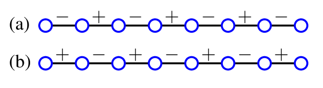
Figure 1: Schematic illustration of the interaction pattern in NN bonds of the lattice, where $+$ denotes repulsive interaction and $-$ denotes attractive interaction.

The structure of this paper is as follows. In Sec. II, we describe the model under consideration and the methodology used to obtain all the results. Sec. III discusses the key findings, focusing on two different natures of the interaction strengths in two nearest-neighbor bonds. Finally, Sec. IV summarizes the main results. The details of the analytical calculations are presented in the Appendix.

II Model and Method

We consider a Hamiltonian for a system of interacting hardcore bosons with dimerized NN interactions as given by

$$H = -t~\sum\limits_{i}({a}^{\dagger}_{i}{a}_{i+1}+\text{H.c.})$$ (1)

$$+V_{1}~\sum\limits_{i\in\text{odd}}(n_{i}-\frac{1}{2})(n_{i+1}-\frac{1}{2})$$

$$+V_{2}~\sum\limits_{i\in\text{even}}(n_{i}-\frac{1}{2})(n_{i+1}-\frac{1}{2}),$$

where $i$ denotes the site index, $a_{i}$ ($a^{\dagger}_{i}$) are the annihilation (creation) operators at site $i$, and $n_{i}=a_{i}^{\dagger}a_{i}$ represents the number operator at site $i$. The parameter $t$ corresponds to the hopping amplitude between NN sites, while $V_{1}$ and $V_{2}$ denote the strengths of the alternating NN interactions. In our numerical calculations presented below, we set $t=1$ which sets the energy scale in the system.

The Hamiltonian given above can be transformed into a spin Hamiltonian by using the Holstein–Primakoff transformation Holstein and Primakoff (1940). This is defined in terms of spin-1/2 operators as

$$S_{i}^{+} = a_{i}^{\dagger}\sqrt{1-a_{i}^{\dagger}a_{i}},~~~~S_{i}^{-}=\sqrt{1-a_{i}^{\dagger}a_{i}}~a_{i},$$

$$S_{i}^{z} = a_{i}^{\dagger}a_{i}-\frac{1}{2},$$ (2)

where the bosonic occupation state $|0\rangle$ and $|1\rangle$ map to the spin states $|\downarrow\rangle$ and $|\uparrow\rangle$ respectively. The Hamiltonian for the spin chain can then be written as

$$H = -2t~\sum\limits_{i}(S_{i}^{x}S_{i+1}^{x}+S_{i}^{y}S_{i+1}^{y})$$ (3)

$$+V_{1}~\sum\limits_{i\in\text{odd}}S_{i}^{z}S_{i+1}^{z}+V_{2}~\sum\limits_{i\in\text{even}}S_{i}^{z}S_{i+1}^{z}.$$

The Hamiltonian in Eq. (3) can also be mapped to a model of interacting spinless fermions using Jordan-Wigner transformation Jordan and Wigner (1928) defined as

$$S_{j}^{-} = e^{i\pi\sum\limits_{k=1}^{j-1}c_{k}^{\dagger}c_{k}}c_{j},~~~~S_{j}^{+}=c_{j}^{\dagger}e^{-i\pi\sum\limits_{k=1}^{j-1}c_{k}^{\dagger}c_{k}},$$

$$S_{j}^{z} = c_{j}^{\dagger}c_{j}~-~\frac{1}{2}~=~n_{i}^{f}~-~\frac{1}{2}.$$ (4)

This mapping leads to a spinless fermionic Hamiltonian which can be written as

$$H = -t~\sum\limits_{i}({c}^{\dagger}_{i}{c}_{i+1}+\text{H.c.})$$ (5)

$$+V_{1}~\sum\limits_{i\in\text{odd}}(n_{i}^{f}-\frac{1}{2})(n_{i+1}^{f}-\frac{1}{2})$$

$$+V_{2}~\sum\limits_{i\in\text{even}}(n_{i}^{f}-\frac{1}{2})(n_{i+1}^{f}-\frac{1}{2}).$$

We have assumed open boundary conditions for this mapping, as will be used throughout this work. With periodic boundary conditions, however, an additional boundary term arises, which depends on the total number of fermions (or total $S_{z}$) in the chain. The above mappings ensure that the models shown in Eqs. 1, 3 and 5 share similar ground state phase diagrams. The results presented below are all obtained by considering the model shown in Eq. 1 which corresponds to a system of hardcore bosons.

The above model has been previously studied using mean-field theory Fisher et al. (1989); Sheshadri et al. (1993); Jaksch et al. (1998); van Oosten et al. (2001), the density-matrix renormalization group (DMRG) White (1992); Schollwöck (2005) method as well as the bosonization approach, for both hardcore bosons and spins  Mondal et al. (2022a); Nigam et al. (2024). These findings highlight that while the non-interacting version of the model remains gapless, introducing a dimerized NN repulsion for hardcore bosons (or dimerized repulsive ZZ exchange interaction for spins) leads to a topological phase and an associated topological phase transition. The topological phase transition occurs as a function of the interaction dimerization which is tuned by fixing the NN interaction strengths for the even (odd) bonds and varying it on the odd (even) bonds of the lattice. This phase transition is marked by a gap-closing point, occurring when the interactions are of equal strengths which guarantees translational symmetry on the lattice. However, the scenario considered in this work is completely different as we assume the NN interaction to be attractive in nature in either all the even or odd bonds (see Fig. 1).

We explore the ground state properties of the system using the DMRG method Cirac et al. (2021); Schollwöck (2011) under open boundary condition (OBC) and for specific cases we use the exact diagonalization (ED) approach with periodic boundary condition (PBC). For the DMRG simulations, we consider a maximum system size of $L=200$ and set the maximum bond dimension to $1000$ to minimize truncation errors. On the other hand, $L=16$ is used for the ED simulations. Unless stated otherwise, all quantities are extrapolated to the thermodynamic limit ($L\rightarrow\infty$) to minimize finite-size effects. We also complement some of our numerical findings through analytical arguments.

III Results

In this section, we discuss our findings in detail. We first present the bulk phase diagram and then analyze the topological properties at half-filling. We also provide the signature of the topological phase through Thouless charge pumping. Subsequently, we analyze the scenario by moving away from half-filling. In the end, we briefly discuss the experimental feasibility of the model.

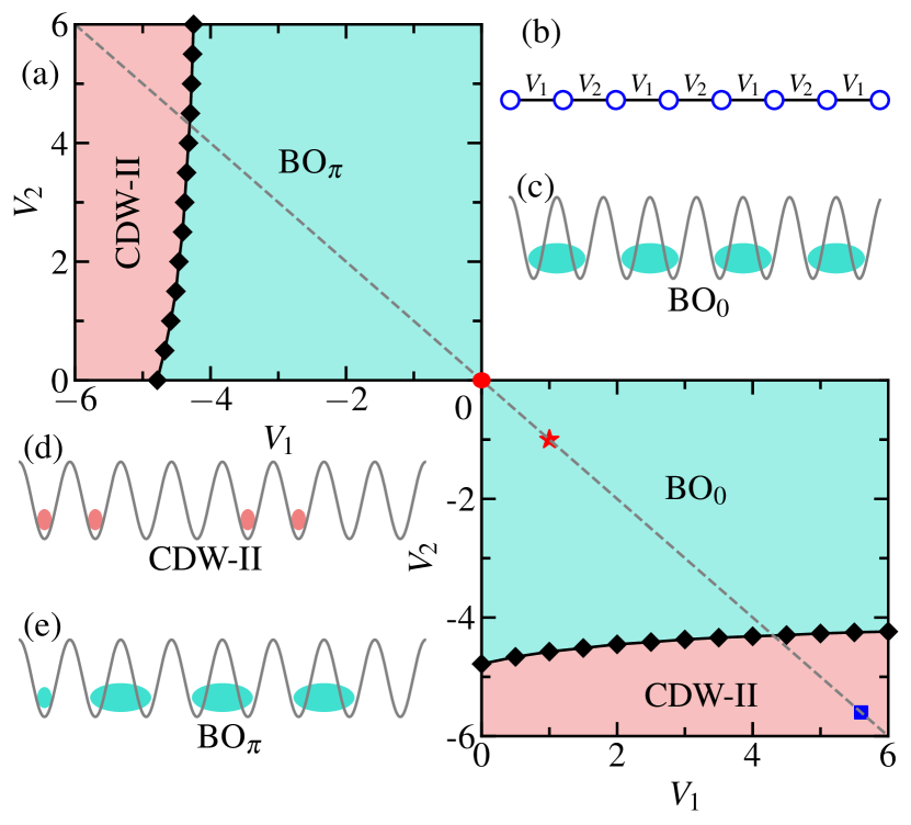
Figure 2: (a) The phase diagram of the model in the $V_{1}-V_{2}$ plane at half-filling shows the BO₀, BO_π and the CDW-II phases. The red circle at the origin depicts the gapless critical point. The black solid diamonds indicate the boundary separating the BO and the CDW-II phases. (b) shows a cartoon diagram depicting the interaction pattern considered. (c), (d) and (e) show the schematics for the BO₀, CDW-II and BO_π phases respectively.

III.1 Phase diagram at half-filling

The ground state phase diagram of the system of hardcore bosons at half-filling is depicted in Fig. 2(a) in the $V_{1}$-$V_{2}$ plane. The upper left (lower right) corner of the figure corresponds to the situation when $V_{1}<0$, $V_{2}>0$ ($V_{1}>0$, $V_{2}<0$). For each case, we numerically find that the entire phase diagram is gapped and there is a gapped-to-gapped transition. In the following, we identify the two gapped phases as the bond order (BO) and the charge-density wave (CDW) phases except at the origin where the system is gapless (denoted by a red circle). We find that for any finite value of $V_{2}$ when $V_{1}=0$, the ground state is a BO phase (the upper left part of the phase diagram). However, as $V_{1}$ is increased on the attractive side, a transition to a CDW phase occurs. This results in a gapped-to-gapped transition as a function of attractive $V_{1}$ for each value of repulsive $V_{2}$. A similar situation is found upon interchanging the nature of the interactions i.e., by making $V_{1}$ repulsive and $V_{2}$ attractive; the corresponding phase diagram is shown in the bottom right corner of Fig. 2(a). In the following, we quantify these phases by computing different relevant physical quantities as a function of $V_{1}=-V_{2}=V$ chosen for simplicity. This corresponds to an exemplary cut drawn in the phase diagram which is denoted by a dashed line in Fig. 2(a). Along this line, when $V<0$, all the odd bonds experience attractive interaction while the even bonds experience repulsive interaction due to the boundary condition (OBC). Conversely, for $V>0$, the odd bonds become repulsive, and even bonds become attractive.

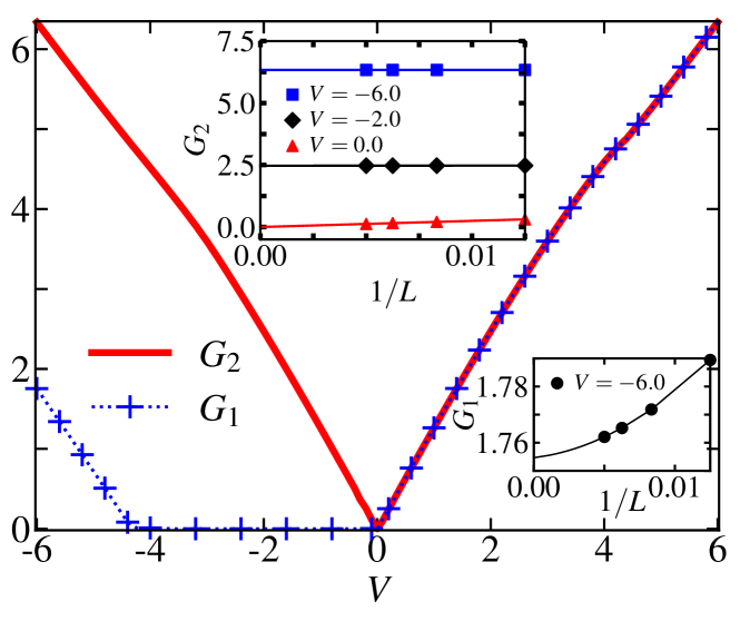
Figure 3: Single-particle excitation gaps $G_{1}$ and $G_{2}$ plotted as a function of $V$ along the dashed line drawn in Fig. 2. $G_{2}$ (solid curve) remains finite in both the gapped phases. $G_{1}$ remains finite in the BO₀ and CDW-II phases and vanishes in the BO_π phase due to the existence of zero-energy edge states. The insets shows the finite-size extrapolation of gaps $G_{1}$ (lower right corner) and $G_{2}$ (upper left corner) in three different parameter regimes corresponding to the gapless phase ($V=0.0$), BO phase ($V=-2.0$) and the CDW phase ($V=-6.0$). In the inset, the solid lines are the fitted curve and the symbols represent the numerical data.

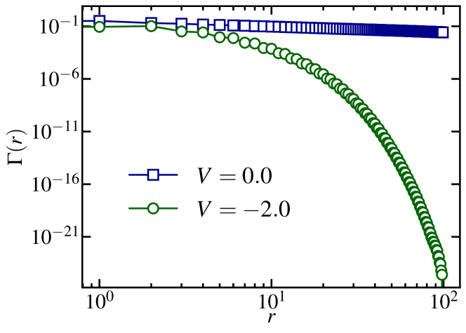
Figure 4: The correlation function $\Gamma(r)$ plotted as a function of distance ($r=|i-j|$) showing power-law and exponential decays for $V=0.0$ and $V=-2.0$ respectively.

To extract the gapped phases in the phase diagram we rely on the particle excitation gaps defined as

$$G_{1}=\mu^{+}-\mu^{-},$$ (6)

where

$$\mu^{+}=E_{N+1}-E_{N}~~~\text{and}~~~\mu^{-}=E_{N}-E_{N-1},$$ (7)

are the chemical potentials corresponding to adding and removing a particle respectively in the system, and $E_{N}$ represents the ground state energy of the system with $N$ bosons. In Fig. 3, we plot the extrapolated values of the gap $G_{1}$ (dotted plus curve) as a function of $V_{1}=-V_{2}=V$. It can be seen that the gap remains finite in the region $V>0$. However, in the region $V\leq 0$, the gap $G_{1}$ vanishes up to a critical $V\sim-4.3$, after which it becomes finite. In the following, we will show that while the vanishing of $G_{1}$ at $V=0$ is due to the gapless nature of the system at that point, for $-4.3\lesssim V<0$, the zero gap is due to the topological nature of the system. Interestingly, when the gap to the next single-particle excitation ($G_{2}$) is calculated using the formula

$$G_{2}=\mu^{+}_{n}-\mu^{-}_{n},$$ (8)

where

$$\mu^{+}_{n}=E_{N+2}-E_{N+1}~~~\text{and}~~~\mu^{-}_{n}=E_{N-1}-E_{N-2},$$ (9)

we find that the system is gapped for all the values of $V\neq 0$ (red solid curve). The insets in Fig. 3 depict the finite-size extrapolation of $G_{1}$ and $G_{2}$ for different values of $V$ (see the figure caption for details). At the gapless point $V=0$, the system exhibits off-diagonal quasi-long-range order which is reflected in the power-law decay of the correlation function

$$\Gamma(r=|i-j|)=\langle a_{i}^{\dagger}a_{j}\rangle$$ (10)

and is plotted in Fig. 4 (blue squares) and this is a signature of the SF phase in one dimension. For comparison, we also show the exponential decay of $\Gamma(r)$ for $V=-2.0$ (green circles) for which the system is gapped.

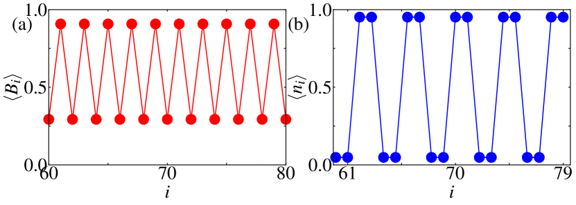
Figure 5: (a) and (b) display the bond energy $\langle B_{i}\rangle$ and on-site particle density $\langle n_{i}\rangle$ for the points $V=2.0$ and $V=5.6$ marked as red star and blue square in the phase diagram Fig. 2, respectively. The finite oscillations in the bond energy for $V=2.0$ signify the presence of the bond ordering in the system , while the finite on-site density oscillations indicate the presence of a CDW ordering exhibiting a density distribution of $...00110011...$ type.

We now turn to quantify the gapped phases. As mentioned already, these are the BO and the CDW phases. The BO phase is characterized by finite dimerization of the particles in the NN bonds. To quantify this feature, we use the bond kinetic energy $\langle B_{i}\rangle$, where $B_{i}=a_{i}^{\dagger}a_{i+1}+\text{H.c.}$, exhibits finite oscillations as a function of the bond index $i$, as shown in Fig. 5 (a) for $V=2.0$ (the point marked as a red star in Fig. 2). At the same time, the CDW order manifests itself as finite oscillations in the real-space density $\langle n_{i}\rangle$ which has the form $\cdots 1100110011\cdots$ as depicted in Fig. 5 (b) for $V=5.6$ (the point marked as a blue square in Fig. 2). This pattern of the density distribution is the signature of a CDW-II phase.

A concrete signature of the BO phase and the CDW-II phase is the presence of finite peaks in their respective structure factors, defined as

$$S_{\text{BO}}(k)=\frac{1}{L^{2}}\sum_{i,j}e^{ik|i-j|}\langle B_{i}B_{j}\rangle,$$ (11)

and

$$S(k)=\frac{1}{L^{2}}\sum_{i,j}e^{ik|i-j|}\langle n_{i}n_{j}\rangle,$$ (12)

where, $S_{\text{BO}}(k)$ is the bond order structure factor and $S(k)$ is the charge-density wave structure factor. To minimize the boundary effects, we consider bond and density correlation functions in the range from $L/4$ to $3L/4$ throughout our calculations. The extrapolated values of $S_{\text{BO}}(k=\pi)$ and $S(k=\pi/2)$ are shown in Fig. 6 as black diamonds and green stars respectively as a function of $V$ (along the dashed line in Fig. 2). The finite values of $S(k=\pi/2)$ for $V\lesssim-4.3$ and $V\gtrsim 4.3$ clearly indicates the CDW-II regions. At the same time, we find that the $S_{\text{BO}}(k=\pi)$ is finite in the region $-4.3<V<4.3$ except at $V=0$ where the system is in the SF phase. However, beyond $V\sim\pm 4.3$, the decrease in $S_{\text{BO}}(k=\pi)$ to smaller values and a sharp increase in $S(k=\pi/2)$ clearly indicates a transition to the CDW-II phase.

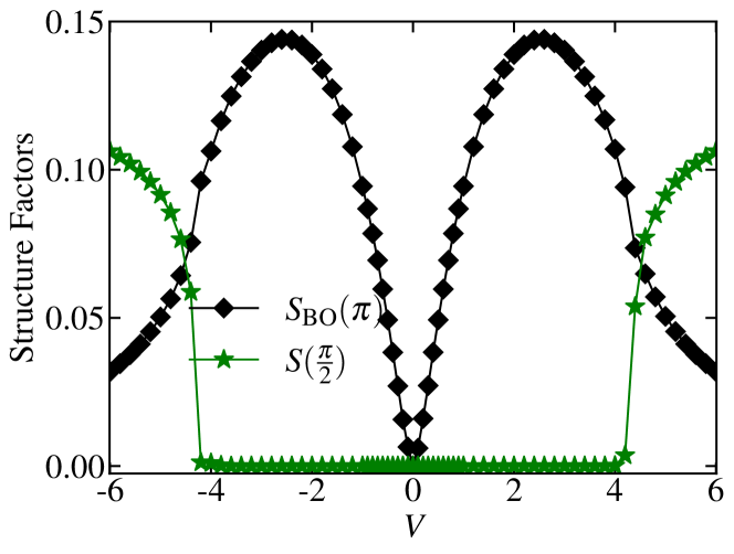
Figure 6: Extrapolated values of $S_{\text{BO}}(\pi)$ (black diamonds) and $S(\pi/2)$ (green stars) as a function of $V$ computed by taking a maximum system size of $L=200$.

To accurately determine the phase transition boundary between the BO and the CDW-II phases, we perform a finite-size scaling of the CDW-II structure factor $S(k=\pi/2)$. Our results show that the BO to CDW-II phase transition belongs to the Ising universality class. The critical point is identified through the appropriate scaling behavior of the CDW-II structure factor

$$S(\pi/2)L^{2\beta/\nu}=F[(V_{1}-V_{1}^{c})L^{1/\nu}],$$ (13)

where $\beta$ and $\nu$ are the magnetization and correlation length critical exponents Mondal et al. (2022a); Mishra et al. (2011). We plot $S(\pi/2)L^{2\beta/\nu}$ as a function of $V_{1}$ for $V_{2}=0$ in Fig. 7 (a) with $\beta=1/8$ and $\nu=1$. The curves for different system sizes are found to cross at the critical point $V_{1}^{c}\sim-4.786$. Moreover, a perfect data collapse for various system sizes is achieved using the scaling function in Eq. (13) at $V_{1}^{c}=-4.786$ as shown in Fig. 7 (b) which confirms the critical point. This approach allows us to map out the entire phase boundary as presented in the upper left part of Fig. 2 (a) (shown as black diamonds). A similar situation is found upon varying $V_{2}$ for each values of $V_{1}$ resulting in the phase boundary shown in the lower right part of Fig. 2 (a).

The upper left (lower right) part of the phase diagram in Fig. 2 (a) shows that as the value of $V_{2}$ ($V_{1})$ is increased, the critical point of the BO to CDW-II transition slowly shifts towards smaller values of attractive $V_{1}$ ($V_{2}$). Moreover, the transition boundary seems to saturate at a particular value of $V_{1}$ ($V_{2}$) in the limit of large $V_{2}$ ($V_{1}$).

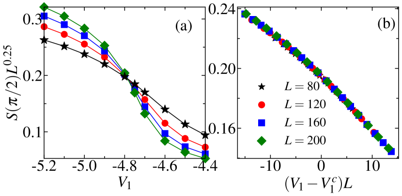
Figure 7: (a) The figure illustrates the finite-size scaling of $S(\pi/2)$ according to Eq. 13 for various values of $V_{1}$ at fixed $V_{2}=0$. The intersection of the curves marks the critical point for the BO to CDW-II phase transition. (b) The scaled $S(\pi/2)$ is plotted against the scaled $V_{1}$, showing a data collapse onto a single curve, confirming $V_{1}^{c}=-4.786$ as the transition point.

The boundary in the limit of large $V_{2}$ ($V_{1}$) can be found using second-order perturbation theory, as shown in Appendix A. For example we find that for $V_{2}\gg t$ and $|V_{1}|$, the location of the boundary between the BO and the CDW-II phases in upper left part of Fig. 2 is given as

$$V_{1}~=~-~4t~-~\frac{2t^{2}}{V_{2}}.$$ (14)

This formula clearly suggests that the critical point saturates to $V_{1}=-4.0$. A similar analysis of the phase transition in the lower right part of Fig. 2 reveals that the critical point for the BO to CDW-II transition saturates to $V_{2}=-4.0$ in the limit of large $V_{1}$.

From the analysis above, it is evident that the entire phase diagram comprises of two distinct gapped phases at half-filling, namely the BO phase and the CDW-II phase. Additionally, a point where the system exhibits features of a SF phase appears at $V_{1}=-V_{2}=0$ which corresponds to the non-interacting limit of the model. In the following we will show that the BO phase in the regime of $V_{1}<0$ and $V_{2}>0$ is topological in nature and the one in the regime of $V_{1}>0$ and $V_{2}<0$ is trivial. We characterize the nature of these phases in detail in the following subsection by taking the same exemplary cut $V_{1}=-V_{2}=V$ as previously mentioned.

III.2 Topological Properties

Here we demonstrate that the two BO phases appearing in the phase diagram (Fig. 2 (a)) on either side of $V_{1}=-V_{2}=V=0$ are topologically distinct, and the transition occurring at $V=0$ is a topological phase transition.

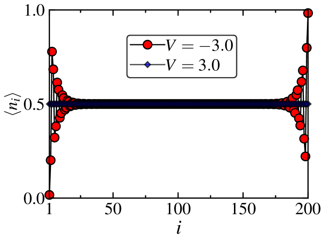
Figure 8: On-site particle density $\langle n_{i}\rangle$ plotted against the site index $i$ in the BO_π and BO₀ phases at $V=-3.0$ (red circles) and $V=3.0$ (blue diamonds), respectively for a system size of $L=200$ sites.

One of the most significant consequences of bulk topology is the presence of degenerate edge modes in OBC. Therefore, as an initial step to characterize the topology of the system, we plot the on-site particle density $\langle n_{i}\rangle$ as a function of the site index for two different BO regimes. Fig. 8 shows the plot of $\langle n_{i}\rangle$ as a function of $i$ for $V=-3.0$ (red circles) and $V=3.0$ (blue diamonds) for a system size $L=200$. The larger values of $\langle n_{i}\rangle$ near the edge sites for $V=-3.0$ compared to uniform density distribution for $V=3.0$ suggests a topological difference between the two types of BO phases.

To concretely establish the topological nature of the BO phase appearing in the regime $-4.3\lesssim V\lesssim 0$ and to characterize the topological phase transition between the two BO phases at $V=0$, we calculate the bulk topological invariant of the system in this regime at various values of $V$ for a system size of $L=16$ using ED. The topological invariant for the interacting system is calculated using twisted boundary conditions, where the hopping strength at the boundary is modified as $t\xrightarrow{}te^{i\theta}$, with $\theta$ being the twist angle Zak (1989); Resta and Sorella (1995). As $\theta$ is varied from $0$ to $2\pi$, the ground state wave function $|\psi(\theta)\rangle$ accumulates a phase, known as the Berry phase ($\gamma$), which is determined using the formula

$$\gamma=i\int_{0}^{2\pi}d\theta~\langle\psi(\theta)|\partial_{\theta}\psi(\theta)\rangle.$$ (15)

The Berry phase is $0$ if the bulk of the system is trivial whereas it is $\pi$ if the bulk is topological in nature. We compute $\gamma$ for different values of $V$ and plot $\gamma/\pi$ as a function of $V$ in Fig. 9(a) (blue diamonds). The plot shows that $\gamma/\pi$ changes from $1$ to $0$ at $V=0$ signifying a phase transition from a topological to a trivial BO phase at $V=0$. Based on the distinct Berry phases of the two BO phases, we denote the topological and the trivial BO phases as BO_π and BO₀ respectively (Fig. 2 (a)).

Another interesting feature of topological systems is the presence of non-local string correlations Dalla Torre et al. (2006); Berg et al. (2008); den Nijs and Rommelse (1989); Tasaki (1991); Hida (1992); Gibson et al. (2011), which can be quantified by a string order parameter defined as

$$O_{\text{str}}(r)~=~-~\langle Z(i)e^{i\frac{\pi}{2}\sum_{j=i+1}^{k-1}Z(j)}Z(k)\rangle,$$ (16)

where $r=|i-j|$ and $Z(i)=1-2a^{\dagger}_{i}a_{i}$. We consider $i=2$ and $k=L-1$ to avoid the edge sites. We calculate $O_{\text{str}}$ for a system with $L=200$ sites and plot in Fig. 9(a) denoted as red stars. It is clear that before $V=0$, the string order parameter is finite and vanishes after $V=0$ which agrees well with the topological invariant (blue diamonds).

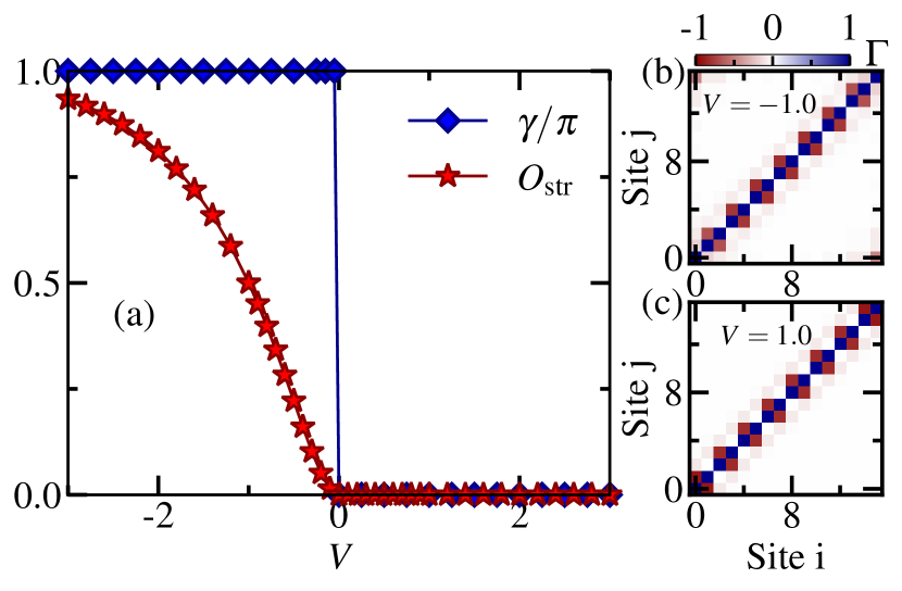
Figure 9: (a) Plots of the winding number $\gamma/\pi$ (blue diamonds) and the string order parameter $O_{\text{str}}$ (red stars) as a function of $V$. The density-density correlation matrix ($\Gamma$) for $V=-1.0$ and $1.0$ shown in (b) and (c), respectively, are calculated using the ED method for a system size of $L=16$ sites.

We also complement our findings by computing the density-density correlation function which is an experimentally relevant quantity de Léséleuc et al. (2019); Mondal et al. (2022a). This is given by

$$\Gamma_{i,j}~=~\langle Z_{i}Z_{j}\rangle~-~\langle Z_{i}\rangle\langle Z_{j}\rangle.$$ (17)

We plot $\Gamma_{i,j}$ for $V=-1.0$ and $V=1.0$ in Figs. 9 (b) and (c) respectively. The presence of finite correlation matrix elements at the two corners, i.e., at the two isolated blue regions at opposite ends of the correlation matrix shown in Fig. 9 (b) indicates the existence of edge states for $V=-1.0$. This clearly signifies the topological character of the BO_π phase. In contrast, Fig. 9 (c) shows no such edge states, indicating the trivial nature of the BO₀ phase for $V=1.0$.

In addition to the above diagonistics, the degeneracy in the entanglement spectrum of the ground state serves as an excellent tool for identifying topological order in a system as it is related to the number of edge excitations in the system Li and Haldane (2008); Yoshida et al. (2014); Turner et al. (2011); Zhou et al. (2023). The entanglement spectrum is obtained by logarithmically rescaling the eigenvalues of the reduced density matrix corresponding to a specific bi-partition of the system. For example, if $l$ is the length of the left block in the DMRG calculation, the reduced density matrix is given by $\rho_{l}=\text{Tr}_{L-l}|\psi\rangle\langle\psi|$, where $|\psi\rangle$ is the ground state wave function. In our case, the singular values at the $l^{th}$ bond in the MPS wave function of the ground state is related to the eigenvalues of the reduced density matrix as $\lambda_{i}=\Lambda_{i}^{2}$, where the $\lambda_{i}$’s are the eigenvalues of the reduced density matrix and the $\Lambda_{i}$’s are the singular values in the MPS wave function. With this idea we calculate the entanglement spectrum as

$$\xi_{i}~=~-~\text{ln}(\Lambda_{i}^{2}),$$ (18)

where the $\Lambda_{i}$’s correspond to the singular values at the central bond of the system in the MPS wave function of the ground state. We plot the lowest four values of the entanglement spectrum $\xi$ as a function of $V$ in Fig. 10 for a system size of $L=200$. We find a two-fold degeneracy in the region $-4.3\lesssim V<0$ apart from which the degeneracy is lifted for all the values of $V$. This indicates the topological nature of the BO ground state in the region $-4.3\lesssim V<0$.

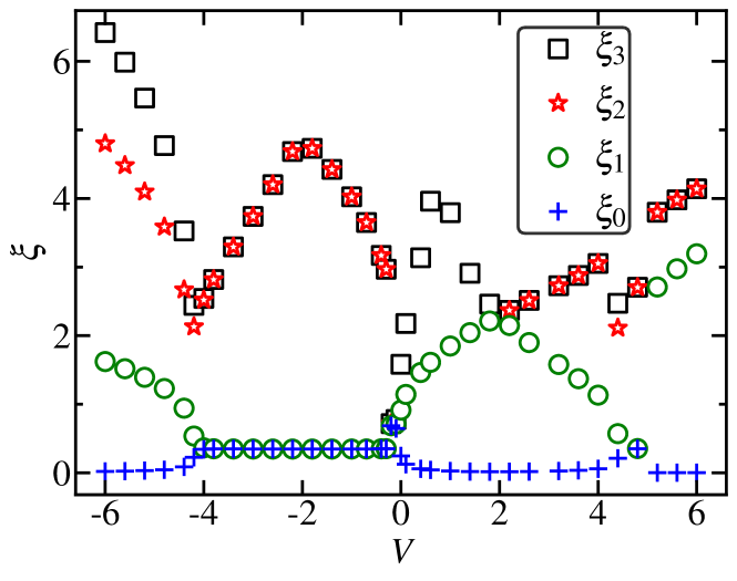
Figure 10: Plot showing the lowest four values of the entanglement spectrum ($\xi_{1},~\xi_{2},~\xi_{3},~\xi_{4}$) as a function of $V$, for $L=200$.

The above analysis concretely establishes a topological phase transition from the BO_π to BO₀ phase as the nature of the NN interactions is altered. In the following, we discuss the signatures of this topological phase transition in the context of Thouless charge pumping that is accessible in existing quantum simulators.

Thouless Charge Pumping

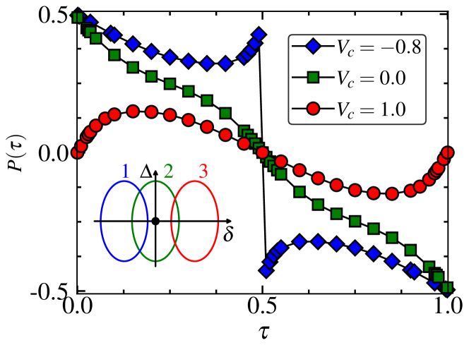
Figure 11: Evolution of the polarization $P(\tau)$ as a function of $\tau$ for a system with $L=200$ sites, shown for three distinct pumping cycles (1, 2, 3) corresponding to different values of $V_{c}$ ($=-0.8,~0.0,~1.0$) as indicated in the inset. In all three cases, we set $A_{\delta}=0.6~\text{and}~A_{\Delta}=0.6$. Blue diamonds, green squares, and red circles represent the polarization changes for cycles 1, 2, and 3, respectively. Robust charge pumping occurs in cycle 2, as it encloses the topological phase transition point $V=0.0$. In contrast, pumping breaks down (since there is a discontinuity in the polarization at $\tau=0.5$) in cycle 1, whereas no charge is pumped during cycle 3.

Here we propose a quantity that dynamically probes and characterizes the aforementioned topological phase called Thouless charge pumping or topological charge pumping (TCP) Thouless (1983). TCP reveals a profound connection between topology and quantum transport, describing the quantized transport of particles through a cyclic and periodic modulation of system parameters without any external bias. The system parameters include one that drives the topological phase transition and an additional inversion symmetry-breaking term, ensuring that the bulk gap remains open throughout the pumping cycle — a necessary condition for particle pumping. The pumping cycle involves the adiabatic evolution of the system from a topological phase to a trivial phase and subsequently back to the initial topological phase again, with the cyclic path encircling the topological phase transition point. Due to the topological nature of the pump, an integer number of particles are transported across the system, and the number of particles transported is directly linked to the topological invariant of the system. Though originally proposed in the context of non-interacting systems, TCP has now been studied in systems of interacting particles. Several theoretical and experimental studies have adopted TCP as one of the crucial tools for revealing the signature of topological phases in both non-interacting as well as interacting systems Lohse et al. (2016); Nakajima et al. (2016); Citro and Aidelsburger (2023); Hayward et al. (2018); Rice and Mele (1982); Citro and Aidelsburger (2023); Asbóth et al. (2016b); Lin et al. (2020); Ke et al. (2017); Argüello-Luengo et al. (2024b); Kuno et al. (2017); Bertok et al. (2022); Mondal et al. (2022b); Hayward et al. (2018); Schweizer et al. (2016); Kraus et al. (2012); Taddia et al. (2017); Wang et al. (2013); Walter et al. (2023); Ke et al. (2020); Padhan et al. (2024); Parida et al. (2024); Jürgensen et al. (2023, 2021). In one dimension, the pumping protocol is given by the celebrated Rice-Mele model. For our system, the corresponding Rice-Mele model is written by adding a symmetry-breaking term, $\Delta$, defining our pumping Hamiltonian, which can now be expressed as

$$H(\tau) = -~t\sum\limits_{i}({a}^{\dagger}_{i}{a}_{i+1}+\text{H.c.})$$ (19)

$$+~(V_{c}-\delta(\tau)\sum\limits_{i}(-1)^{i}(n_{i}-\frac{1}{2})(n_{i+1}-\frac{1}{2})$$

$$+~\Delta(\tau)\sum\limits_{i}(-1)^{i}n_{i},$$

where $\tau$ is the pumping parameter. The parameter $\Delta$ ensures that the bulk gap remains open throughout the pumping cycle. $V_{c}$ is the origin of the pumping cycle in the $\delta-\Delta$ plane. $\delta(\tau)=A_{\delta}\text{cos}(2\pi\tau)$ and $\Delta(\tau)=A_{\Delta}\text{sin}(2\pi\tau)$ periodically modulate the nearest-neighbor interaction and the staggered potential term respectively. We consider three pumping cycles corresponding to three different values of $V_{c}$ as shown in the inset of Fig. 11. The parameter sets ($V_{c},A_{\delta},A_{\Delta}$) for these three cycles are taken to be ($-0.8t,0.6t,0.6t$), ($0.0t,0.6t,0.6t$) and ($1.0t,0.6t,0.6t$) for cycle 1,2, and 3 respectively. One should expect that pumping can only happen for cycle $2$ (green continuous line) as it winds around the topological phase transition point $V=0$. To study the TCP, we calculate a quantity called polarization given by

$$P(\tau)~=~\frac{1}{L}~\sum\limits_{i=1}^{L}~\langle\psi(\tau)|(i-i_{0})n_{i}|\psi(\tau)\rangle,$$ (20)

where $i_{0}=(L+1)/2$ for a system of $L=200$ sites for all the three cycles. Here $\psi(\tau)$ represents the ground state wave function of the Hamiltonian defined in Eq. 19. The amount of charge pumped ($Q$) in a cycle is given as

$$Q=\int_{0}^{1}d\tau~\partial_{\tau}P(\tau).$$ (21)

Fig. 11 clearly demonstrates a smooth change in the polarization from $0.5$ to $-0.5$, indicating a total charge transfer of $|Q|=1$ for cycle 2. This signifies robust and quantized pumping occurring in cycle 2 as it encloses the gap-closing topological phase transition point as mentioned earlier. In contrast, cycle 1 exhibits a breakdown of pumping (due to the appearance of a discontinuity in the polarization), while cycle 3 shows no pumping at all Hayward et al. (2018). This analysis complements the topological phase transition between the two BO phases shown in the phase diagram [Fig. 2(a)].

III.3 Away from half-filling

After studying the ground state phase diagram in both the regimes of interactions at half-filling, we now extend our analysis to explore the system across all densities. For this purpose, we again focus on the same cut through the phase diagram that corresponds to the $V_{1}=-V_{2}=V$ line (gray dashed line in Fig. 2 (a)) as mentioned earlier. The phase diagram of the system in the $V-\mu$ plane is depicted in Fig. 12. The gapped phases at $\rho=1/2$, namely the BO and the CDW-II phases, appear in the regions with $V>0$ and $V<0$ and are separated by a vertical dashed line. At $V=0$ the gap vanishes and it corresponds to the topological phase transition point between the BO_π and BO₀ phases at half-filling as discussed earlier. The gray regions on the upper and lower sides of the gapped phases are the gapless phases which appear for densities away from half-filling. The upper and lower white regions are the completely filled and completely empty (vacuum) states with $\rho=1$ and $\rho=0$ respectively. The boundaries of these phases are determined from the change in the chemical potential $\mu$ as the particle density $\rho$ of the system is defined. For this purpose, we analyze the features from the $\rho$ vs $\mu$ plot which are shown in Figs. 13 (a) and (b) for two exemplary values of $V=-3.0$ and $V=-5.5$ respectively.

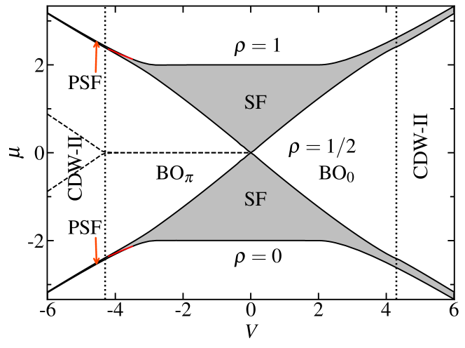
Figure 12: The phase diagram of the model in $V-\mu$ plane by taking $V_{1}=-V_{2}=V$ under open boundary condition. Dashed lines indicate the presence of edge states. The white regions in the middle enclosed by gray regions correspond to gapped phases at half-filling, while the white regions at $\rho=0$ and $\rho=1$ represent the empty and fully occupied states, respectively. Gray-shaded regions denote gapless phases, which are further classified based on excitation type: regions with single-particle excitations are identified as the SF phase, while regions with two-particle excitations correspond to the PSF phase. Red solid lines mark the boundary between the SF and PSF phases.

Here we plot the bulk and the edge densities defined as

$$\rho_{b}=\frac{1}{L-2}\sum\limits_{i=2}^{L-1}\langle n_{i}\rangle,$$ (22)

and

$$\rho_{e}=\frac{1}{2}[\langle n_{1}\rangle+\langle n_{L}\rangle],$$ (23)

using red solid lines and blue dashed lines respectively. The large plateaus in $\rho_{b}$ (red solid lines) in both the figures at $\rho=1/2$ is due to the gapped phases, and the shoulders across the plateaus correspond to the gapless phases. The length of the plateau at $\rho=1/2$ determines the gap at this filling, and the end points of the plateau determine the boundaries of the gapped phase appearing at $\rho=1/2$ corresponding to the particular cut in the phase diagram shown in Fig. 12. Interestingly, there are two degenerate mid-gap zero energy modes appearing in the phase diagram starting from $V=0$ to $V\sim-4.3$ surpassing which these states become energetic, and these are indicated by the dashed lines at the center of the phase diagram. These are the signatures of edge states which have already been discussed in the previous section; they appear here as a consequence of the bulk topology. The degeneracy persists in the topological BO phase which then becomes non-degenerate because of the transition into the trivial CDW-II phase.

This signature of edge states can be captured from the $\rho-\mu$ plot shown in Fig. 13. The jump in $\rho_{e}$ by 1 when the bulk is gapped in Fig. 13 (a) at $\mu=0$ is an indication of the presence of two zero energy edge states in this parameter regime. Similarly, the jump in $\rho_{e}$ by 0.5 in Fig. 13 (b) while the bulk is gapped at finite $\mu$ represents the presence of finite-energy edge states.

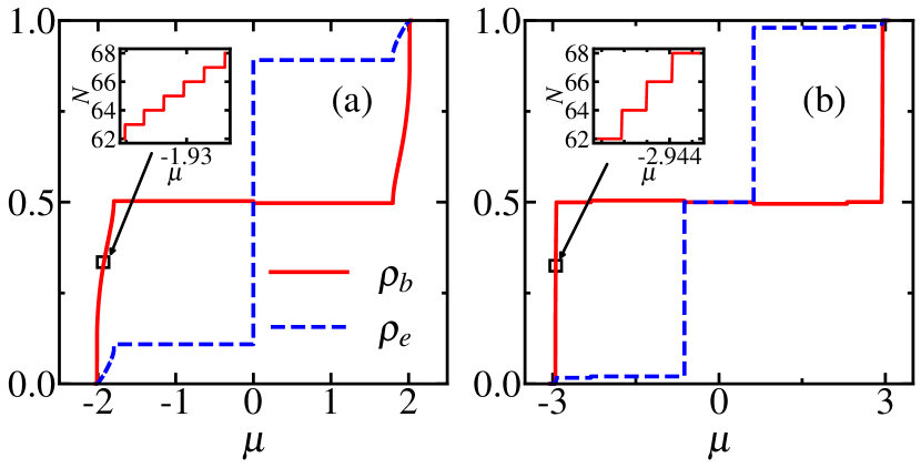
Figure 13: The figure depicts the bulk and edge densities represented by $\rho_{b}$ (red solid lines) and $\rho_{e}$ (blue dashed lines) respectively as a function of $\mu$, for two different cuts through the phase diagram shown in Fig. 12: (a) $V=-3.0$ and (b) $V=-5.5$ for a system size of $L=200$. This shows the nature of bulk phases (gapped or gapless) when the edge states are being filled in different parameter regimes. The inset shows the number of particles filled $N$ as a function of chemical potential $\mu$. The single-particle and two-particle jumps in the insets of (a) and (b) represent the existence of SF and PSF phases respectively.

Figure 14: The SF correlation function $\Gamma\text{(}r)$ and the PSF correlation function $\Gamma^{\text{2}}(r)$ plotted as a function of the distance ($r=|i-j|$) on a log-log scale at $\rho=0.25$ for $V=5.5$ for a system with size $L=200$. To avoid the boundary effects we only consider the lattice sites from $L/4$ to $3L/4$.

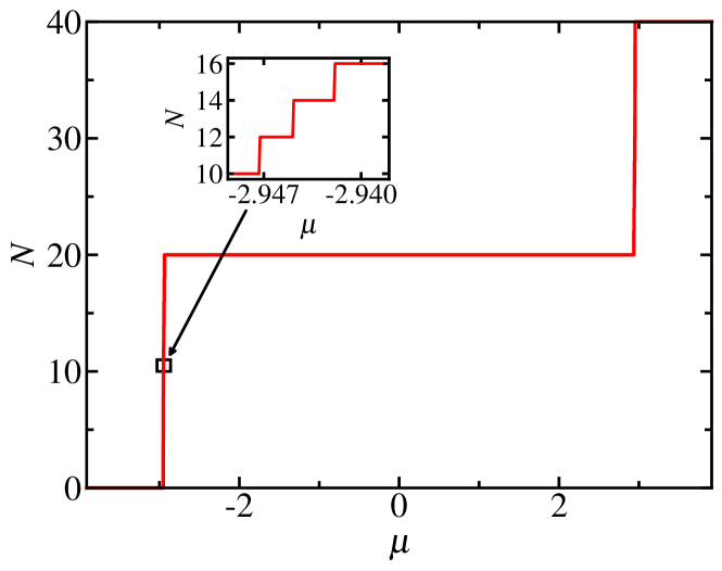
Figure 15: The figure shows the number of particles filled as a function of the chemical potential $\mu$ for $V=5.5$ under PBC for a system size of $L=40$. The inset shows the zoomed region of the red curve which is indicated by an arrow. The two-particle jump is clear from the inset which is a signature of the PSF phase.

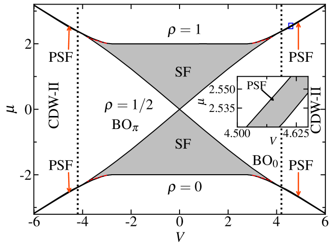
Figure 16: Phase diagram of the model in the $V-\mu$ plane by taking $V_{1}=-V_{2}=V$ with periodic boundary condition. All the phase boundaries are extrapolated by taking a maximum system size of $L=60$. All the regions have the usual meaning as mentioned in the phase diagram shown in Fig. 12. The red dashed lines mark the boundary between the SF and the PSF phases. The rectangular region marked in blue in the upper right part of the diagram is enlarged in the inset to show that the $\rho=0$ and $\rho=1/2$ regions are separated by a finite gray region which carries PSF order.

We now examine the phases away from commensurate densities. As evident from the phase diagram [Fig. 12] as well as from the $\rho-\mu$ curve [Fig. 13], the regions away from half-filling correspond to gapless phases. In some regions, the excitations are of single-particle type representing an SF phase, whereas in some other regions, the excitations are pair excitations representing a pair superfluid (PSF) phase. The PSF phase arises due to strong attractive interactions that favor the formation of bound nearest-neighbor pairs. To distinguish between the SF and PSF phases, we plot the particle number $N$ as a function of the chemical potential $\mu$ in the inset of Fig. 13, focusing on the region marked by the black rectangle for a system size of $L=200$ sites. The single-particle jump in $N$ with increase in $\mu$ for $V=-3.0$ (inset in Fig. 13 (a)) shows the presence of an SF phase, whereas the two-particle jump for $V=-5.5$ (inset in Fig. 13 (b)) shows the existence of the PSF phase. These features can also be understood from analytical arguments discussed in Appendix B. The jumps in $\rho_{b}$ in steps of $1$ occurring when $\mu$ is slightly more than $-2.0$ (Fig. 13(a)) is due to single particles appearing in the bulk when $\mu$ increases above $-2.0$ as discussed in Appendix B (see Eq. (36)). The jumps in $\rho_{b}$ in steps of $2$ occurring when $\mu$ increases above $-2.94$ (Fig. 13(b)) is due to the appearance of two-particle bound states in the bulk. If we substitute $V=-5.5$ in Eq. (51), it gives a threshold equal to about $-2.95$ which matches well with the numerical results.

The SF and PSF boundaries are separated by the red lines in the phase diagram shown in Fig. 12. Note that a similar SF-PSF transition line is observed for the $V>0$ case; however, it is not seen from the $\rho$-$\mu$ curve obtained with OBC because of the choice of the boundary condition and the repulsive interaction in the first and the last bonds. More details can be found in Appendix B. Nevertheless, the PSF nature can still be verified by examining the behavior of the PSF correlation function which is given by

$$\Gamma^{2}(r=|i-j|)=\langle a_{i}^{\dagger}a_{i+1}^{\dagger}a_{j}a_{j+1}\rangle.$$ (24)

The algebraic decay of the PSF correlation function $\Gamma^{2}(r)$ (green circles) in Fig. 14 for $V=5.5$ shows the existence of a PSF phase in this parameter regime. For comparison, we also plot the SF correlation function $\Gamma(r)$ (blue squares) defined in Eq. 10 which shows an exponential decay confirming the existence of the PSF order in the system.

To address this issue arising because of OBC, periodic boundary conditions (PBC) can be employed, allowing for a clearer examination of the $\rho$-$\mu$ curve. Hence, we analyze the $\rho-\mu$ curve at $V=5.5$ by employing PBC for a system size of $L=40$ and show the result in Fig. 15. The presence of a two-particle jump away from half-filling under PBC confirms the existence of the PSF phase in the bulk. The jumps occur due to the appearance of two-particle bound states in the bulk as discussed in Appendix B (see Eq. (51)). In contrast, under OBC, a single-particle density jump is observed even within the PSF region. Owing to this specific artifact introduced by the boundary condition, the phase diagram in Fig. 12 is not symmetric about $V=0$ although the bulk physics remains the same on the two sides. We provide a qualitative understanding of this picture in Appendix B; see the discussion around Eqs. (57) and (58) of hole or particle end modes which appear for $V>2.0$.

To resolve this issue numerically, we once again compute the bulk phase diagram by implementing the PBC; this is presented in Fig. 16. The maximum system size in this case has been taken to be $L=60$, and all the phase boundaries are extrapolated to the thermodynamic limit. The mid-gap edge modes are now absent in the $V<0$ regime, as the implementation of PBC eliminates edge states. Now the phase diagram exhibits complete reflection symmetry about $V=0$. Additionally, there are four red lines in the phase diagram that mark the boundaries between the SF and PSF phases. One can clearly see that at higher interaction strengths, the boundary region between the vacuum state ($\rho=0$) and the half-filled state ($\rho=1/2$) (or between the fully occupied state ($\rho=1$) and the half-filled state) appears narrow and seemingly merge to a single line. However, a finite intermediate gray region remains, consisting of two-particle excitations, which defines the PSF phase. To illustrate this more clearly, the inset shown in Fig. 16 provides a zoomed-in view of the blue rectangular region, confirming the existence of a gapless phase between the two gapped phases.

In Appendix B, we present an understanding of the phase boundary below the fully filled state with $\rho=1$ in Fig. 16. We show that the boundary is given by $\mu=2t$ if $|V|\leq 2\sqrt{2}t$ which results from one-hole states, and by

$$\mu~=~t~\left[\sqrt{\frac{V^{2}}{4t^{2}}~-~1}~+~\frac{1}{\sqrt{\frac{V^{2}}{4t^{2}}~-~1}}\right],$$ (25)

if $|V|>2\sqrt{2}t$ which results from two-hole bound states and these boundaries agree well with the numerical calculations (Fig. 16). Similar expressions hold for the phase boundary above the empty state with $\rho=0$ in Fig. 16 (see Eq. (51)).

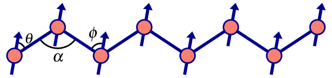
Figure 17: Array of dipoles representing the model under consideration. The angles $\theta$ and $\phi$ control the strength and signs of the interactions $V_{1}$ and $V_{2}$ respectively.

The above analysis provides a comprehensive study of the phases emerging at all densities. Apart from the fully empty and fully occupied states, a gapped phase appears at half-filling, as previously discussed. At all other densities, the system exhibits gapless nature. In certain regions, single-particle excitations dominate, characterizing the SF phase, while other regions are dominated by bound pair excitations and hence called the PSF phase. In the following, we discuss how such a model can be realized in experiments.

III.4 Experimental scheme

In this subsection, we briefly discuss the possible experimental realization of the model with tunable NN interactions. As already mentioned in the introduction, the NN interactions have been successfully realized in various quantum simulators. Here, we show that a properly arranged array of dipolar atoms can be a suitable choice to achieve the tunability of the potentials $V_{1}$ and $V_{2}$ that is required to observe the topological phase transition. In Fig. 17, we show that the atoms arranged in the zig-zag pattern can selectively allow the atoms to hop between the NN sites while the hopping to the next-nearest-neighbor sites can be avoided by increasing the angle $\alpha$. We assume that the dipoles can be oriented in the $XY$-plane. The dipole-dipole interaction between the two dipoles is given by

$$V_{dd}=\frac{q^{2}}{4\pi\epsilon_{0}{r}^{3}}(1-3\text{cos}^{2}(\Phi)),$$ (26)

where $\Phi$ is the angle made by the dipoles with the line joining the two dipoles Giovanazzi et al. (2002). Consequently, the nearest-neighbor interaction strengths are given by

$$V_{1}=\frac{q^{2}}{4\pi\epsilon_{0}{r}^{3}}(1-3\text{cos}^{2}(\theta)),$$

$$~~~\text{and}~~~V_{2}=\frac{q^{2}}{4\pi\epsilon_{0}{r}^{3}}(1-3\text{cos}^{2}(\phi)),$$ (27)

where $\theta$ and $\phi$ are the angles specified in Fig. 17. Hence to tune the interaction between the NN dipoles as required by the model under consideration, $V_{1}$ and $V_{2}$ can be tuned by uniformly rotating all the dipoles. Here, we set $\alpha=2\theta_{m}$, where $\theta_{m}$ is the ”magic angle” — the angle at which the dipole-dipole interaction strength vanishes which is given by $\text{cos}^{-1}(\frac{1}{\sqrt{3}})$. In this configuration, the angle $\phi$ is given by $\pi+\theta-2\theta_{m}$. By externally controlling the dipole orientation in the $XY$-plane, it is possible to adjust $\theta$, which in turn modifies $\phi$. It then becomes possible to simultaneously set the angles $\theta$ and $\phi$ to be $\theta_{m}$ and $\pi-\theta_{m}$ which makes both the nearest-neighbor interaction strengths zero. Fig. 18 presents the variation of $V_{1}$ and $V_{2}$ as a function of $\theta$, assuming the prefactor in Eq. 27 to be unity. Initially, $V_{1}$ (red squares) is negative, while $V_{2}$ (green circles) is positive. As $\theta$ reaches $\theta_{m}$, both interactions vanish. Further increasing $\theta$ beyond this point reverses their signs. This controlled variation of interaction strengths enables the realization of topological phase transitions in the system.

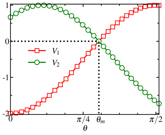
Figure 18: Tunable NN interactions $V_{1}$ (red squares) and $V_{2}$ (green circles) as a function of $\theta$.

IV Conclusion

We have numerically investigated the ground state properties of a one-dimensional lattice of hardcore bosons or spinless fermions with tunable NN interactions. While the non-interacting counterpart of the system is a trivial gapless phase, we have showed that by allowing attractive and repulsive interactions on the alternate NN bonds of the lattice, a topological phase can be established. We have also showed that by tuning the NN interaction appropriately, a topological to trivial phase transition occurs at a critical point where the interactions vanish. Apart from this, we have also obtained a symmetry broken phase for stronger interaction strengths. While we have revealed that the bulk of the topological and the trivial phases exhibit finite bond ordering, the symmetry broken phase exhibits a CDW order. We have obtained the phase diagram depicting these phases and the transitions between them at half-filling with tunable NN interactions. Furthermore, by extending our analysis beyond half-filling, we have explored the phase diagram at all densities and identified both single-particle and bound-pair excitations at incommensurate fillings, leading to the superfluid (SF) and pair-superfluid (PSF) phases. We have also provided analytical arguments for specific scenarios in support of the numerical results. Finally, we discussed the experimental feasibility of realizing the model under consideration in quantum simulation platforms, such as Rydberg atom and ultracold atomic set ups.

V Acknowledgements

We thank Immanuel Bloch, Rejish Nath, Subhro Bhattacharjee and Ashirbad Padhan for useful discussions. We also thank Biswajit Paul and Sanchayan Banerjee for useful comments on the manuscript. We acknowledge discussions in the ICTS program titled “A Hundred Years of Quantum Mechanics” (code: ICTS/qm100-2025/01). T.M. acknowledges support from the Science and Engineering Research Board (SERB), Government of India, through project No. MTR/2022/000382 and No. STR/2022/000023. D.S. acknowledges support from SERB, Government of India, through project No. JBR/2020/000043.

Appendix A Degenerate perturbation theory for the anisotropic limits

In this Appendix we will provide a derivation of Eq. (14) in the main text. Given the Hamiltonian in Eq. (3), we will assume that $V_{2}\gg t$ and $|V_{1}|$, and will go up to second order in perturbation theory. We begin by considering only the terms with $V_{2}$ which constitutes the unperturbed Hamiltonian. The ground state of this part of the Hamiltonian in Eq. (3) has a large degeneracy: for every even value of $i$, the pair of spins on sites $i$ and $i+1$ must be either in the state $|\uparrow_{i}\downarrow_{i+1}\rangle$ or in the state $|\downarrow_{i}\uparrow_{i+1}\rangle$. We therefore define a new lattice with sites labeled as $j=i/2$ and spin-1/2 operators ${\vec{\tau}}_{j}$ which sit at the bond $(i,i+1)$ of the original lattice such that the above two states correspond to $\tau_{j}^{z}=1$ and $\tau_{j}^{z}=-1$ respectively.

In the space of degenerate ground states described above, we see that the $V_{1}$ term in Eq. (3) effectively acts as $-(V_{1}/4)\tau_{j}^{z}\tau_{j+1}^{z}$. For instance, acting on the state $|\tau_{j}^{z}=1,\tau_{j+1}^{z}=1\rangle=|\uparrow_{i}\downarrow_{i+1}\uparrow_{i+2}\downarrow_{i+3}\rangle$, the term $V_{1}S_{i+1}^{z}S_{i+2}^{z}$ gives $(-V_{1}/4)|\tau_{j}^{z}=1,\tau_{j+1}^{z}=1\rangle$.

Next, the term in Eq. (3) of the form

$$-~2t~(S_{i}^{x}S_{i+1}^{x}~+~S_{i}^{y}S_{i+1}^{y})~=~-~t~(\sigma_{i}^{+}\sigma_{i+1}^{-}~+~\sigma_{i}^{-}\sigma_{i+1}^{+})$$ (28)

flips the state $\tau_{j}^{z}=1$ to $\tau_{j}^{z}=-1$, and vice versa. Hence this term effectively acts as $-t~\tau_{j}^{x}$.

However, the term in Eq. (3) of the form

$$-~2t~(S_{i-1}^{x}S_{i}^{x}~+~S_{i-1}^{y}S_{i}^{y})~=~-~t~(\sigma_{i-1}^{+}\sigma_{i}^{-}~+~\sigma_{i-1}^{-}\sigma_{i}^{+}),$$ (29)

where $i$ is even, does not have any matrix elements between states in the space of degenerate ground states. But this term contributes to second order as follows. Acting on the state $|\tau_{j-1}^{z}=1,\tau_{j}^{z}=1\rangle=|\uparrow_{i-2}\downarrow_{i-1}\uparrow_{i}\downarrow_{i+1}\rangle$, the term in Eq. (29) gives $-t|\uparrow_{i-2}\uparrow_{i-1}\downarrow_{i}\downarrow_{i+1}\rangle$ which is an excited state whose energy is $V_{2}$ larger than the energy of the degenerate ground states. Another application of Eq. (29) brings the excited state back to $|\tau_{j-1}^{z}=1,\tau_{j}^{z}=1\rangle$, with a coefficient equal to $(-t)^{2}/(-V_{2})=-t^{2}/V_{2}$ as given by second-order perturbation theory; the energy denominator equal to $-V_{2}$ comes from $E_{ground}-E_{excited}$. A similar terms appears for the state $|\tau_{j-1}^{z}=-1,\tau_{j}^{z}=-1\rangle$. However, no such terms appear for the states $|\tau_{j-1}^{z}=1,\tau_{j}^{z}=-1\rangle$ and $|\tau_{j-1}^{z}=-1,\tau_{j}^{z}=1\rangle$ since Eq. (29) gives zero on these states. Hence, Eq. (29) gives rise to a term in the effective Hamiltonian given by $(-t^{2}/(2V_{2}))(\mathbb{I}~+~\tau_{j-1}^{z}\tau_{j}^{z})$.

Hence, ignoring some constants, the low-energy effective Hamiltonian is given by

$$H_{eff}~=~\sum_{j}~[(-~\frac{V_{1}}{4}-\frac{t^{2}}{2V_{2}})~\tau_{j-1}^{z}\tau_{j}^{z}~-~t~\tau_{j}^{x}].$$ (30)

This describes the transverse field Ising model. It is well-known that this model has a second-order phase transition when the coefficients of the two terms in Eq. (30) are equal in magnitude, i.e., when $t=|(V_{1}/4)+(t^{2}/(2V_{2}))|$. For $V_{1}<0$, this gives the line

$$V_{1}~=~-~4t~-~\frac{2t^{2}}{V_{2}}.$$ (31)

This is Eq. (14) in the main text.

Appendix B Boundaries close to $\rho=1$ and $\rho=0$

In this Appendix, we will consider the Hamiltonian in Eq. (1) with $V_{1}=-V_{2}=V$, and add a chemical potential term $-\mu\sum_{i}n_{i}$. We will derive the forms of the boundaries close to the completely filled and completely empty states that we see in Fig. 12 for open boundary conditions and Fig. 16 for periodic boundary conditions.

To understand Fig. 16, we will consider an $L$-site system with periodic boundary conditions so that momentum eigenstates can be defined. The fully occupied state in which the number of particles is $L$ is an eigenstate of Eq. (1) with energy equal to $E_{0}=-\mu L$. Next, we consider a one-hole state in which the number of particles is $L-1$. Defining a state with a hole located at site $j$ as $|j\rangle$, we find that

$$H|j\rangle~=~-\mu(L-1)~|j\rangle~-~t~|j-1\rangle~-~t|j+1\rangle.$$ (32)

Next, we define a momentum eigenstate as

$$|k\rangle~=~\sum_{i}~e^{ijk}~|j\rangle.$$ (33)

We then find that $H|k\rangle=-(\mu L-\mu+2t\cos k)|k\rangle$. Subtracting the energy $E_{0}$ of the fully occupied state, we see that the dispersion of a single hole is given by

$$E_{1}(k)~=~\mu~-~2t~\cos k.$$ (34)

This implies that the one-hole state has lower energy than the fully occupied state below the line

$$\mu~=~2t.$$ (35)

This gives the boundary below the region with $\rho=1$ for $|V|\ll t$; this is consistent with what we see in Fig. 12. Next, after doing a particle-hole transformation, $n_{i}\to 1-n_{i}$ for all $i$, we can use arguments similar to the ones presented above to show that the boundary above the region $\rho=0$ in Fig. 16 is given by

$$\mu~=~-~2t$$ (36)

due to the appearance of one-particle states. We would like to note here that although Eqs. (35) and (36) were derived assuming periodic boundary conditions, these equations will also give the thresholds for one-hole or one-particle excitations to appear in the bulk even when the system has open boundary conditions.

We now turn to two-hole states. For $|V|\gg t$, we can first ignore the terms with $t$ in Eq. (1). We then see that there is a two-hole bound state in which only the sites $i$ and $i+1$ are empty, where $i$ is odd if $V<0$ and is even if $V>0$. The difference of the energy of this state from $E_{0}$ is $2\mu-|V|$ (this is less than the lowest one-hole state which lies at $\mu-2t$). Hence the two-hole state has less energy than the fully occupied state below the line $2\mu=|V|$, i.e.,

$$\mu~=~\frac{|V|}{2}.$$ (37)

This gives the boundary below the region with $\rho=1$ for $|V|\gg t$; this is also consistent with Fig. 12. (Note that the lowest energy of a one-hole state is at $\mu-2t$ which lies above the two-hole state at $2\mu-|V|$ if $\mu<|V|/2$).

We will now study the form of a two-hole bound state when $|V|$ may be of the same order as $t$. A two-hole state will have sites $n_{1}$ and $n_{2}$ empty, where $n_{1}<n_{2}$; we will denote this state as $|n_{1},n_{2}\rangle$. (In this discussion, it will be convenient to consider an infinitely large system so that we do not have to worry about boundary conditions). We will now consider a bound state which has a center-of-mass momentum $k$; this lies in the range $[-2\pi,2\pi]$. The wave function of such a state can be written as

$$|k\rangle_{B}~=~\sum_{n_{1}<n_{2}}~e^{ik(n_{1}+n_{2})/2}~f(n_{1},n_{2})|n_{1},n_{2}\rangle,$$ (38)

where $f(n_{1},n_{2})$ depends on the difference $m=n_{2}-n_{1}$ (where $m\geq 1$) and on whether $n_{1}$ is even or odd. This leads us to define

$$f(n_{1},n_{2}) = \alpha(m=n_{2}-n_{1})~~{\rm if}~~n_{1}~~{\rm is~odd},$$ (39)

$$= \beta(m=n_{2}-n_{1})~~{\rm if}~~n_{1}~~{\rm is~even}.$$

Then the eigenvalue equation obtained from Eq. (1), $H|k\rangle_{B}=E_{2}(k)|k\rangle_{B}$ leads to the equations

$$-t~[\alpha(m+1)e^{ik/2}~+~\alpha(m-1)e^{-ik/2}$$

$$+~\beta(m+1)e^{-ik/2}~+~\beta(m-1)e^{ik/2}]$$

$$=~E_{2}~\alpha(m)~~{\rm for}~~m\geq 2,$$

$$-t~[\beta(m+1)e^{ik/2}~+~\beta(m-1)e^{-ik/2}$$

$$+~\alpha(m+1)e^{-ik/2}~+~\alpha(m-1)e^{ik/2}]$$

$$=~E_{2}~\beta(m)~~{\rm for}~~m\geq 2,$$

$$-t~[\alpha(2)e^{ik/2}~+~\beta(2)e^{-ik/2}]~+~V~\alpha(1)~=~E_{2}~\alpha(1),$$

$$-t~[\beta(2)e^{ik/2}~+~\alpha(2)e^{-ik/2}]~-~V~\beta(1)~=~E_{2}~\beta(1).$$

(40)

The form of Eqs. (40) is invariant under the transformation

$$\alpha(m) \to (-1)^{m}~\beta(m),$$

$$\beta(m) \to (-1)^{m}~\alpha(m),$$

$$E \to -~E.$$ (41)

Hence, if there is a solution of Eqs. (40) with energy $E$, there must be another solution with energy $-E$.

For every value of $k$, we can numerically solve Eqs. (40) and see if there are bound state solutions; these must satisfy $|\alpha(m)|$ and $|\beta(m)|\to 0$ as $m\to\infty$. If a bound state exists, we denote its energy as $E_{2}(k)$. (Then there will be another bound state with energy $-E_{2}(k)$ as discussed above). As $|V|$ is increased from zero, we find that bound states first appears at $k=0$. Further, if bound states are present for a range of values of $k$, its energy is the lowest at $k=0$. We will therefore concentrate on the case $k=0$ henceforth. Eqs. (42) then take the form

$$-t~[\alpha(m+1)~+~\alpha(m-1)~+~\beta(m+1)~+~\beta(m-1)]$$

$$=~E_{2}(0)~\alpha(m)~~{\rm for}~~m\geq 2,$$

$$-t~[\beta(m+1)~+~\beta(m-1)~+~\alpha(m+1)~+~\alpha(m-1)]$$

$$=~E_{2}(0)~\beta(m)~~{\rm for}~~m\geq 2,$$

$$-t~[\alpha(2)~+~\beta(2)]~+~V~\alpha(1)~=~E_{2}(0)~\alpha(1),$$

$$-t~[\beta(2)~+~\alpha(2)]~-~V~\beta(1)~=~E_{2}(0)~\beta(1).$$ (42)

These equations imply the following:

$$\alpha(m)~=~\beta(m)~~{\rm for}~~m\geq 2,$$ (43)

and

$$\alpha(1) = -~\frac{2t\alpha(2)}{E_{2}(0)~-~V},$$

$$\beta(1) = -~\frac{2t\alpha(2)}{E_{2}(0)~+~V}.$$ (44)

Substituting Eq. (43) in the first equation in Eq. (42) with $m\geq 3$, we obtain

$$-2t~[\alpha(m+1)~+~\alpha(m-1)]~=~E_{2}(0)~\alpha(m)~~{\rm for}~~m\geq 3.$$ (45)

Ignoring an overall prefactor for $\alpha(m)$, the solution of this is given by

$$\alpha(m)~=~e^{-\lambda m}~~{\rm and}~~E_{2}(0)~=~-2t~(e^{\lambda}~+~e^{-\lambda}),$$ (46)

where $\lambda$ must be real and positive in order to have a normalizable state. Then the first equation in Eq. (42) with $m=2$ gives

$$\alpha(1)~+~\beta(1)~=~2e^{-\lambda}.$$ (47)

Combining Eqs. (44), (46) and (47), we obtain

$$e^{\lambda}~=~\sqrt{\frac{V^{2}}{4t^{2}}~-~1}.$$ (48)

Hence the lowest energy of a two-hole bound state is

$$E_{2}(k=0)~=~-2t~\left[\sqrt{\frac{V^{2}}{4t^{2}}~-~1}~+~\frac{1}{\sqrt{\frac{V^{2}}{4t^{2}}~-~1}}\right].$$ (49)

As argued above, there must be another bound state at $k=0$ with the energy $-E_{2}(k=0)$.

Since a bound state must have $\lambda>0$, Eq. (48) implies that a bound state appears only if $|V|>2\sqrt{2}t$. Since the right hand side of Eq. (49) is always less than $-2t$, we see that the lowest energy excitations around the fully occupied state are two-hole bound states rather than one-hole states, if $|V|>2\sqrt{2}t$.

Upon subtracting the energy of the fully occupied state, we find that the minimum energy of a two-hole bound state is equal to $2\mu+E_{2}(k=0)$. Hence the boundary below the region $\rho=1$ is given by the condition $\mu=-(1/2)E_{2}(k=0)$, namely,

$$\mu~=~t~\left[\sqrt{\frac{V^{2}}{4t^{2}}~-~1}~+~\frac{1}{\sqrt{\frac{V^{2}}{4t^{2}}~-~1}}\right],$$ (50)

provided that $|V|>2\sqrt{2}t$. (Note that for $|V|\gg t$, Eq. (50) reduces to $\mu=|V|/2$ as we found earlier).

Finally, after doing a particle-hole transformation, $n_{i}\to 1-n_{i}$, we can use similar arguments as above to find the boundary above the region $\rho=0$ in Fig. 12. We find that this given by

$$\mu = -~2t~~{\rm for}~~|V|~\leq~2\sqrt{2}~t,$$ (51)

$$= -~t~\left[\sqrt{\frac{V^{2}}{4t^{2}}~-~1}~+~\frac{1}{\sqrt{\frac{V^{2}}{4t^{2}}~-~1}}\right]$$

$$~{\rm for}~~|V|~>~2\sqrt{2}~t.$$

Once again, we note that although Eqs. (50) and (51) were derived assuming periodic conditions, they also give thresholds for two-hole or two-particle excitations to appear in the bulk for a system with open boundary conditions.

We will now provide an understanding of Fig. 12 obtained for open boundary conditions. Looking closely at the boundary below the region $\rho=1$ for $V>2$, we see a difference between the cases of periodic boundary conditions (Fig. 16) and open boundary conditions (Fig. 12). This difference arises due to the appearance of a hole state which is localized near the end of an open system when the interaction $V_{1}=V$ at the last bond (connecting sites 1 and 2) is positive; we will call this state the hole end mode. To understand this quantitatively, we consider a state with the wave function

$$|\psi\rangle_{B}~=~\sum_{n=1}^{\infty}~f_{n}~|n\rangle,$$ (52)

where $|n\rangle$ denotes a state in which only site $n$ is empty, and $n=1$ denotes the leftmost site of the system. From Eq. (1), we find that the diagonal term of the Hamiltonian has a value which is $V/2$ less at $n=1$ as compared to all other values of $n\geq 2$. Next, including the hopping term proportional to $-t$, we effectively obtain a tight-binding model with a negative on-site potential $-V/2$ at site 1 and hopping amplitude $-t$ between neighboring sites $n$ and $n+1$. Eq. (52) and the eigenvalue condition $H|\psi\rangle_{B}=E_{B}|\psi\rangle_{B}$ lead to the equations

$$-~\frac{V}{2}~f_{1}~-~t~f_{2} = E_{B}~f_{1},$$

$$-~t~(f_{n-1}~+~f_{n+1}) = E_{B}~f_{n}~~{\rm for}~~n\geq 2.$$ (53)

The solution of the second equation in Eqs. (53) is given by

$$f_{n} = e^{-\lambda n},$$

$$E_{B} = -t~(e^{\lambda}~+~e^{-\lambda}),$$ (54)

where $\lambda$ is real and positive. Substituting this in the first equation in Eqs. (53), we obtain

$$e^{\lambda}~=~\frac{V}{2t},$$ (55)

which implies that the hole end mode appears only if $V>2t$. The energy of this mode is given by

$$E_{B}~=~-~\frac{V}{2}~-~\frac{2t^{2}}{V}.$$ (56)

This energy will be less than that of the state with all sites occupied if the chemical potential lies below the line

$$\mu~=~\frac{V}{2}~+~\frac{2t^{2}}{V},$$ (57)

provided that $V>2t$. Comparing Eq. (50) for a two-hole bound state (which applies if $V>2\sqrt{2}t$) and Eq. (50) for a hole end mode (which applies if $V>2t)$, we find that $\mu$ given by Eq. (57) always lies above $\mu$ given by Eq. (50). Thus, if $\mu$ is gradually decreased from large values, the boundary below the region $\rho=1$ is determined by the hole end mode before the two-hole bound states enter the picture.

Once again, we can do a particle-hole transformation and show that the boundary above the region $\rho=0$ in Fig. 12 for $V>2$ is determined by the appearance of a particle end mode. The boundary is found to lie at

$$\mu~=~-~\frac{V}{2}~-~\frac{2t^{2}}{V}.$$ (58)

References

- Hasan and Kane (2010) M. Z. Hasan and C. L. Kane, “Colloquium: Topological insulators,” Rev. Mod. Phys. 82, 3045–3067 (2010).
- Senthil (2015a) T. Senthil, “Symmetry-protected topological phases of quantum matter,” Annual Review of Condensed Matter Physics 6, 299–324 (2015a).
- Rachel (2018) Stephan Rachel, “Interacting topological insulators: a review,” Reports on Progress in Physics 81, 116501 (2018).
- von Klitzing (2017) Klaus von Klitzing, “Metrology in 2019,” Nature Physics 13, 198–198 (2017).
- Senthil (2015b) T. Senthil, “Symmetry-protected topological phases of quantum matter,” Annual Review of Condensed Matter Physics 6, 299–324 (2015b).
- Fidkowski and Kitaev (2011) Lukasz Fidkowski and Alexei Kitaev, “Topological phases of fermions in one dimension,” Phys. Rev. B 83, 075103 (2011).
- Pollmann et al. (2010) Frank Pollmann, Ari M. Turner, Erez Berg, and Masaki Oshikawa, “Entanglement spectrum of a topological phase in one dimension,” Phys. Rev. B 81, 064439 (2010).
- Gu and Wen (2009) Zheng-Cheng Gu and Xiao-Gang Wen, “Tensor-entanglement-filtering renormalization approach and symmetry-protected topological order,” Phys. Rev. B 80, 155131 (2009).
- Chen et al. (2012) Xie Chen, Zheng-Cheng Gu, Zheng-Xin Liu, and Xiao-Gang Wen, “Symmetry-protected topological orders in interacting bosonic systems,” Science 338, 1604–1606 (2012).
- Pachos and Simon (2014) Jiannis K Pachos and Steven H Simon, “Focus on topological quantum computation,” New Journal of Physics 16, 065003 (2014).
- Su et al. (1979) W. P. Su, J. R. Schrieffer, and A. J. Heeger, “Solitons in polyacetylene,” Phys. Rev. Lett. 42, 1698–1701 (1979).
- Asbóth et al. (2016a) János K. Asbóth, László Oroszlány, and András Pályi, “The su-schrieffer-heeger (ssh) model,” in A Short Course on Topological Insulators: Band Structure and Edge States in One and Two Dimensions (Springer International Publishing, Cham, 2016) pp. 1–22.
- Anastasiadis et al. (2022) Adamantios Anastasiadis, Georgios Styliaris, Rajesh Chaunsali, Georgios Theocharis, and Fotios K. Diakonos, “Bulk-edge correspondence in the trimer su-schrieffer-heeger model,” Phys. Rev. B 106, 085109 (2022).
- Li et al. (2014) Linhu Li, Zhihao Xu, and Shu Chen, “Topological phases of generalized su-schrieffer-heeger models,” Phys. Rev. B 89, 085111 (2014).
- Pérez-González et al. (2019) Beatriz Pérez-González, Miguel Bello, Álvaro Gómez-León, and Gloria Platero, “Interplay between long-range hopping and disorder in topological systems,” Phys. Rev. B 99, 035146 (2019).
- Ahmadi et al. (2020) N. Ahmadi, J. Abouie, and D. Baeriswyl, “Topological and nontopological features of generalized su-schrieffer-heeger models,” Phys. Rev. B 101, 195117 (2020).
- Atala et al. (2013) Marcos Atala, Monika Aidelsburger, Julio T. Barreiro, Dmitry Abanin, Takuya Kitagawa, Eugene Demler, and Immanuel Bloch, “Direct measurement of the zak phase in topological bloch bands,” Nature Physics 9, 795 (2013).
- Nakajima et al. (2016) Shuta Nakajima, Takafumi Tomita, Shintaro Taie, Tomohiro Ichinose, Hideki Ozawa, Lei Wang, Matthias Troyer, and Yoshiro Takahashi, “Topological thouless pumping of ultracold fermions,” Nature Physics 12, 296 (2016).
- Lohse et al. (2016) M. Lohse, C. Schweizer, O. Zilberberg, M. Aidelsburger, and I. Bloch, “A thouless quantum pump with ultracold bosonic atoms in an optical superlattice,” Nature Physics 12, 350–354 (2016).
- Mukherjee et al. (2017) Sebabrata Mukherjee, Alexander Spracklen, Manuel Valiente, Erika Andersson, Patrik Öhberg, Nathan Goldman, and Robert R. Thomson, “Experimental observation of anomalous topological edge modes in a slowly driven photonic lattice,” Nature Communications 8, 13918 (2017).
- Lu et al. (2014) Ling Lu, John D. Joannopoulos, and Marin Soljačić, “Topological photonics,” Nature Photonics 8, 821–829 (2014).
- Thatcher et al. (2022) Luke Thatcher, Parker Fairfield, Lázaro Merlo-Ramírez, and Juan M Merlo, “Experimental observation of topological phase transitions in a mechanical 1d-ssh model,” Physica Scripta 97, 035702 (2022).
- Meier et al. (2016) Eric J. Meier, Fangzhao Alex An, and Bryce Gadway, “Observation of the topological soliton state in the su–schrieffer–heeger model,” Nature Communications 7, 13986 (2016).
- Xie et al. (2019) Dizhou Xie, Wei Gou, Teng Xiao, Bryce Gadway, and Bo Yan, “Topological characterizations of an extended su–schrieffer–heeger model,” npj Quantum Information 5, 55 (2019).
- Kitagawa et al. (2012) Takuya Kitagawa, Matthew A. Broome, Alessandro Fedrizzi, Mark S. Rudner, Erez Berg, Ivan Kassal, Alán Aspuru-Guzik, Eugene Demler, and Andrew G. White, “Observation of topologically protected bound states in photonic quantum walks,” Nature Communications 3, 882 (2012).
- Leder et al. (2016) Martin Leder, Christopher Grossert, Lukas Sitta, Maximilian Genske, Achim Rosch, and Martin Weitz, “Real-space imaging of a topologically protected edge state with ultracold atoms in an amplitude-chirped optical lattice,” Nature Communications 7, 13112 (2016).
- de Léséleuc et al. (2019) Sylvain de Léséleuc, Vincent Lienhard, Pascal Scholl, Daniel Barredo, Sebastian Weber, Nicolai Lang, Hans Peter Büchler, Thierry Lahaye, and Antoine Browaeys, “Observation of a symmetry-protected topological phase of interacting bosons with rydberg atoms,” Science 365, 775–780 (2019).
- Le et al. (2020) Nguyen H. Le, Andrew J. Fisher, Neil J. Curson, and Eran Ginossar, “Topological phases of a dimerized fermi–hubbard model for semiconductor nano-lattices,” npj Quantum Information 6, 24 (2020).
- Jörg et al. (2024) Christina Jörg, Marius Jürgensen, Sebabrata Mukherjee, and Mikael C. Rechtsman, “Optical control of topological end states via soliton formation in a 1d lattice,” Nanophotonics (2024), doi:10.1515/nanoph-2024-0401.
- Li et al. (2013) Xiaopeng Li, Erhai Zhao, and W. Vincent Liu, “Topological states in a ladder-like optical lattice containing ultracold atoms in higher orbital bands,” Nature Communications 4, 1523 (2013).
- Taddia et al. (2017) Luca Taddia, Eyal Cornfeld, Davide Rossini, Leonardo Mazza, Eran Sela, and Rosario Fazio, “Topological fractional pumping with alkaline-earth-like atoms in synthetic lattices,” Phys. Rev. Lett. 118, 230402 (2017).
- Grusdt et al. (2013) Fabian Grusdt, Michael Höning, and Michael Fleischhauer, “Topological edge states in the one-dimensional superlattice bose-hubbard model,” Phys. Rev. Lett. 110, 260405 (2013).
- Manmana et al. (2012) Salvatore R. Manmana, Andrew M. Essin, Reinhard M. Noack, and Victor Gurarie, “Topological invariants and interacting one-dimensional fermionic systems,” Phys. Rev. B 86, 205119 (2012).
- Yoshida et al. (2018) Tsuneya Yoshida, Ippei Danshita, Robert Peters, and Norio Kawakami, “Reduction of topological classification in cold-atom systems,” Phys. Rev. Lett. 121, 025301 (2018).
- Ryu and Hatsugai (2002) Shinsei Ryu and Yasuhiro Hatsugai, “Topological origin of zero-energy edge states in particle-hole symmetric systems,” Phys. Rev. Lett. 89, 077002 (2002).
- Di Liberto et al. (2016) M. Di Liberto, A. Recati, I. Carusotto, and C. Menotti, “Two-body physics in the su-schrieffer-heeger model,” Phys. Rev. A 94, 062704 (2016).
- Di Liberto et al. (2017) M. Di Liberto, A. Recati, I. Carusotto, and C. Menotti, “Two-body bound and edge states in the extended ssh bose-hubbard model,” The European Physical Journal Special Topics 226, 2751–2762 (2017).
- Nakagawa et al. (2018) Masaya Nakagawa, Tsuneya Yoshida, Robert Peters, and Norio Kawakami, “Breakdown of topological thouless pumping in the strongly interacting regime,” Phys. Rev. B 98, 115147 (2018).
- Fraxanet et al. (2022) Joana Fraxanet, Daniel González-Cuadra, Tilman Pfau, Maciej Lewenstein, Tim Langen, and Luca Barbiero, “Topological quantum critical points in the extended bose-hubbard model,” Phys. Rev. Lett. 128, 043402 (2022).
- Wang et al. (2015) Da Wang, Shenglong Xu, Yu Wang, and Congjun Wu, “Detecting edge degeneracy in interacting topological insulators through entanglement entropy,” Phys. Rev. B 91, 115118 (2015).
- Barbiero et al. (2018) L. Barbiero, L. Santos, and N. Goldman, “Quenched dynamics and spin-charge separation in an interacting topological lattice,” Phys. Rev. B 97, 201115 (2018).
- Ye et al. (2016) Bing-Tian Ye, Liang-Zhu Mu, and Heng Fan, “Entanglement spectrum of su-schrieffer-heeger-hubbard model,” Phys. Rev. B 94, 165167 (2016).
- Kuno (2019) Yoshihito Kuno, “Phase structure of the interacting su-schrieffer-heeger model and the relationship with the gross-neveu model on lattice,” Phys. Rev. B 99, 064105 (2019).
- Montorsi et al. (2022) A. Montorsi, U. Bhattacharya, Daniel González-Cuadra, M. Lewenstein, G. Palumbo, and L. Barbiero, “Interacting second-order topological insulators in one-dimensional fermions with correlated hopping,” Phys. Rev. B 106, L241115 (2022).
- Julià-Farré et al. (2024) Sergi Julià-Farré, Javier Argüello-Luengo, Loïc Henriet, and Alexandre Dauphin, “Quantized thouless pumps protected by interactions in dimerized rydberg tweezer arrays,” Phys. Rev. A 110, 023328 (2024).
- Delplace et al. (2011) P. Delplace, D. Ullmo, and G. Montambaux, “Zak phase and the existence of edge states in graphene,” Phys. Rev. B 84, 195452 (2011).
- Zhou et al. (2023) Xiaofan Zhou, Jian-Song Pan, and Suotang Jia, “Exploring interacting topological insulator in the extended su-schrieffer-heeger model,” Phys. Rev. B 107, 054105 (2023).
- Li and Haldane (2008) Hui Li and F. D. M. Haldane, “Entanglement spectrum as a generalization of entanglement entropy: Identification of topological order in non-abelian fractional quantum hall effect states,” Phys. Rev. Lett. 101, 010504 (2008).
- Julià-Farré et al. (2022) Sergi Julià-Farré, Daniel González-Cuadra, Alexander Patscheider, Manfred J. Mark, Francesca Ferlaino, Maciej Lewenstein, Luca Barbiero, and Alexandre Dauphin, “Revealing the topological nature of the bond order wave in a strongly correlated quantum system,” Phys. Rev. Res. 4, L032005 (2022).
- Argüello-Luengo et al. (2024a) Javier Argüello-Luengo, Manfred J. Mark, Francesca Ferlaino, Maciej Lewenstein, Luca Barbiero, and Sergi Julià-Farré, “Stabilization of Hubbard-Thouless pumps through nonlocal fermionic repulsion,” Quantum 8, 1285 (2024a).
- Dalla Torre et al. (2006) Emanuele G. Dalla Torre, Erez Berg, and Ehud Altman, “Hidden order in 1d bose insulators,” Phys. Rev. Lett. 97, 260401 (2006).
- Rossini and Fazio (2012) Davide Rossini and Rosario Fazio, “Phase diagram of the extended bose–hubbard model,” New Journal of Physics 14, 065012 (2012).
- Berg et al. (2008) Erez Berg, Emanuele G. Dalla Torre, Thierry Giamarchi, and Ehud Altman, “Rise and fall of hidden string order of lattice bosons,” Phys. Rev. B 77, 245119 (2008).
- Greschner et al. (2020) Sebastian Greschner, Suman Mondal, and Tapan Mishra, “Topological charge pumping of bound bosonic pairs,” Phys. Rev. A 101, 053630 (2020).
- Padhan et al. (2024) Ashirbad Padhan, Suman Mondal, Smitha Vishveshwara, and Tapan Mishra, “Interacting bosons on a su-schrieffer-heeger ladder: Topological phases and thouless pumping,” Phys. Rev. B 109, 085120 (2024).
- Mondal et al. (2022a) Suman Mondal, Ashirbad Padhan, and Tapan Mishra, “Realizing a symmetry protected topological phase through dimerized interactions,” Phys. Rev. B 106, L201106 (2022a).
- Parida et al. (2024) Rajashri Parida, Ashirbad Padhan, and Tapan Mishra, “Interaction driven topological phase transitions of hardcore bosons on a two-leg ladder,” Phys. Rev. B 110, 165110 (2024).
- Nigam et al. (2024) Harsh Nigam, Ashirbad Padhan, Diptiman Sen, Tapan Mishra, and Subhro Bhattacharjee, “Phases and phase transitions in a dimerized spin- xxz chain,” (2024), arXiv:2408.14474 [cond-mat.str-el] .
- Sompet et al. (2022) Pimonpan Sompet, Sarah Hirthe, Dominik Bourgund, Thomas Chalopin, Julian Bibo, Joannis Koepsell, Petar Bojović, Ruben Verresen, Frank Pollmann, Guillaume Salomon, Christian Gross, Timon A. Hilker, and Immanuel Bloch, “Realizing the symmetry-protected haldane phase in fermi–hubbard ladders,” Nature 606, 484–488 (2022).
- Li et al. (2023) Yuqing Li, Yunfei Wang, Hongxing Zhao, Huiying Du, Jiahui Zhang, Ying Hu, Feng Mei, Liantuan Xiao, Jie Ma, and Suotang Jia, “Interaction-induced breakdown of chiral dynamics in the su-schrieffer-heeger model,” Phys. Rev. Res. 5, L032035 (2023).
- Jürgensen et al. (2023) Marius Jürgensen, Sebabrata Mukherjee, Christina Jörg, and Mikael C. Rechtsman, “Quantized fractional thouless pumping of solitons,” Nature Physics 19, 420–426 (2023).
- Jürgensen et al. (2021) Marius Jürgensen, Sebabrata Mukherjee, and Mikael C. Rechtsman, “Quantized nonlinear thouless pumping,” Nature 596, 63–67 (2021).
- Holstein and Primakoff (1940) T. Holstein and H. Primakoff, “Field dependence of the intrinsic domain magnetization of a ferromagnet,” Phys. Rev. 58, 1098–1113 (1940).
- Jordan and Wigner (1928) P. Jordan and E. Wigner, “über das paulische äquivalenzverbot,” Zeitschrift für Physik 47, 631–651 (1928).
- Fisher et al. (1989) Matthew P. A. Fisher, Peter B. Weichman, G. Grinstein, and Daniel S. Fisher, “Boson localization and the superfluid-insulator transition,” Phys. Rev. B 40, 546–570 (1989).
- Sheshadri et al. (1993) K. Sheshadri, H. R. Krishnamurthy, R. Pandit, and T. V. Ramakrishnan, “Superfluid and insulating phases in an interacting-boson model: Mean-field theory and the rpa,” Europhysics Letters 22, 257 (1993).
- Jaksch et al. (1998) D. Jaksch, C. Bruder, J. I. Cirac, C. W. Gardiner, and P. Zoller, “Cold bosonic atoms in optical lattices,” Phys. Rev. Lett. 81, 3108–3111 (1998).
- van Oosten et al. (2001) D. van Oosten, P. van der Straten, and H. T. C. Stoof, “Quantum phases in an optical lattice,” Phys. Rev. A 63, 053601 (2001).
- White (1992) Steven R. White, “Density matrix formulation for quantum renormalization groups,” Phys. Rev. Lett. 69, 2863–2866 (1992).
- Schollwöck (2005) U. Schollwöck, “The density-matrix renormalization group,” Rev. Mod. Phys. 77, 259–315 (2005).
- Cirac et al. (2021) J. Ignacio Cirac, David Pérez-García, Norbert Schuch, and Frank Verstraete, “Matrix product states and projected entangled pair states: Concepts, symmetries, theorems,” Rev. Mod. Phys. 93, 045003 (2021).
- Schollwöck (2011) Ulrich Schollwöck, “The density-matrix renormalization group in the age of matrix product states,” Annals of Physics 326, 96–192 (2011), january 2011 Special Issue.
- Mishra et al. (2011) Tapan Mishra, Juan Carrasquilla, and Marcos Rigol, “Phase diagram of the half-filled one-dimensional -- model,” Phys. Rev. B 84, 115135 (2011).
- Zak (1989) J. Zak, “Berry’s phase for energy bands in solids,” Phys. Rev. Lett. 62, 2747–2750 (1989).
- Resta and Sorella (1995) R. Resta and S. Sorella, “Many-body effects on polarization and dynamical charges in a partly covalent polar insulator,” Phys. Rev. Lett. 74, 4738–4741 (1995).
- den Nijs and Rommelse (1989) Marcel den Nijs and Koos Rommelse, “Preroughening transitions in crystal surfaces and valence-bond phases in quantum spin chains,” Phys. Rev. B 40, 4709–4734 (1989).
- Tasaki (1991) Hal Tasaki, “Quantum liquid in antiferromagnetic chains: A stochastic geometric approach to the haldane gap,” Phys. Rev. Lett. 66, 798–801 (1991).
- Hida (1992) Kazuo Hida, “Crossover between the haldane-gap phase and the dimer phase in the spin-1/2 alternating heisenberg chain,” Phys. Rev. B 45, 2207–2212 (1992).
- Gibson et al. (2011) Sandra J. Gibson, R. Meyer, and Gennady Y. Chitov, “Numerical study of critical properties and hidden orders in dimerized spin ladders,” Phys. Rev. B 83, 104423 (2011).
- Yoshida et al. (2014) Tsuneya Yoshida, Robert Peters, Satoshi Fujimoto, and Norio Kawakami, “Characterization of a topological mott insulator in one dimension,” Phys. Rev. Lett. 112, 196404 (2014).
- Turner et al. (2011) Ari M. Turner, Frank Pollmann, and Erez Berg, “Topological phases of one-dimensional fermions: An entanglement point of view,” Phys. Rev. B 83, 075102 (2011).
- Thouless (1983) D. J. Thouless, “Quantization of particle transport,” Phys. Rev. B 27, 6083–6087 (1983).
- Citro and Aidelsburger (2023) Roberta Citro and Monika Aidelsburger, “Thouless pumping and topology,” Nature Reviews Physics 5, 87–101 (2023).
- Hayward et al. (2018) A. Hayward, C. Schweizer, M. Lohse, M. Aidelsburger, and F. Heidrich-Meisner, “Topological charge pumping in the interacting bosonic rice-mele model,” Phys. Rev. B 98, 245148 (2018).
- Rice and Mele (1982) M. J. Rice and E. J. Mele, “Elementary excitations of a linearly conjugated diatomic polymer,” Phys. Rev. Lett. 49, 1455–1459 (1982).
- Asbóth et al. (2016b) János K. Asbóth, László Oroszlány, and András Pályi, “Adiabatic charge pumping, rice-mele model,” in A Short Course on Topological Insulators: Band Structure and Edge States in One and Two Dimensions (Springer International Publishing, Cham, 2016) pp. 55–68.
- Lin et al. (2020) Ling Lin, Yongguan Ke, and Chaohong Lee, “Interaction-induced topological bound states and thouless pumping in a one-dimensional optical lattice,” Phys. Rev. A 101, 023620 (2020).
- Ke et al. (2017) Yongguan Ke, Xizhou Qin, Yuri S. Kivshar, and Chaohong Lee, “Multiparticle wannier states and thouless pumping of interacting bosons,” Phys. Rev. A 95, 063630 (2017).
- Argüello-Luengo et al. (2024b) Javier Argüello-Luengo, Manfred J. Mark, Francesca Ferlaino, Maciej Lewenstein, Luca Barbiero, and Sergi Julià-Farré, “Stabilization of Hubbard-Thouless pumps through nonlocal fermionic repulsion,” Quantum 8, 1285 (2024b).
- Kuno et al. (2017) Yoshihito Kuno, Keita Shimizu, and Ikuo Ichinose, “Various topological mott insulators and topological bulk charge pumping in strongly-interacting boson system in one-dimensional superlattice,” New Journal of Physics 19, 123025 (2017).
- Bertok et al. (2022) E. Bertok, F. Heidrich-Meisner, and A. A. Aligia, “Splitting of topological charge pumping in an interacting two-component fermionic rice-mele hubbard model,” Phys. Rev. B 106, 045141 (2022).
- Mondal et al. (2022b) Suman Mondal, Eric Bertok, and Fabian Heidrich-Meisner, “Phonon-induced breakdown of thouless pumping in the rice-mele-holstein model,” Phys. Rev. B 106, 235118 (2022b).
- Schweizer et al. (2016) C. Schweizer, M. Lohse, R. Citro, and I. Bloch, “Spin pumping and measurement of spin currents in optical superlattices,” Phys. Rev. Lett. 117, 170405 (2016).
- Kraus et al. (2012) Yaacov E. Kraus, Yoav Lahini, Zohar Ringel, Mor Verbin, and Oded Zilberberg, “Topological states and adiabatic pumping in quasicrystals,” Phys. Rev. Lett. 109, 106402 (2012).
- Wang et al. (2013) Lei Wang, Matthias Troyer, and Xi Dai, “Topological charge pumping in a one-dimensional optical lattice,” Phys. Rev. Lett. 111, 026802 (2013).
- Walter et al. (2023) Anne-Sophie Walter, Zijie Zhu, Marius Gächter, Joaquín Minguzzi, Stephan Roschinski, Kilian Sandholzer, Konrad Viebahn, and Tilman Esslinger, “Quantization and its breakdown in a hubbard–thouless pump,” Nature Physics 19, 1471–1475 (2023).
- Ke et al. (2020) Yongguan Ke, Janet Zhong, Alexander V. Poshakinskiy, Yuri S. Kivshar, Alexander N. Poddubny, and Chaohong Lee, “Radiative topological biphoton states in modulated qubit arrays,” Phys. Rev. Res. 2, 033190 (2020).
- Giovanazzi et al. (2002) Stefano Giovanazzi, Axel Görlitz, and Tilman Pfau, “Tuning the dipolar interaction in quantum gases,” Phys. Rev. Lett. 89, 130401 (2002).