Spectral decomposition-assisted multi-study
factor analysis

Abstract

This article focuses on covariance estimation for multi-study data. Popular approaches employ factor-analytic terms with shared and study-specific loadings that decompose the variance into (i) a shared low-rank component, (ii) study-specific low-rank components, and (iii) a diagonal term capturing idiosyncratic variability. Our proposed methodology estimates the latent factors via spectral decompositions and infers the factor loadings via surrogate regression tasks, avoiding identifiability and computational issues of existing alternatives. Reliably inferring shared vs study-specific components requires novel developments that are of independent interest. The approximation error decreases as the sample size and the data dimension diverge, formalizing a blessing of dimensionality. Conditionally on the factors, loadings and residual error variances are inferred via conjugate normal-inverse gamma priors. The conditional posterior distribution of factor loadings has a simple product form across outcomes, facilitating parallelization. We show favorable asymptotic properties, including central limit theorems for point estimators and posterior contraction, and excellent empirical performance in simulations. The methods are applied to integrate three studies on gene associations among immune cells.

Keywords: Data integration; Factor analysis; High-dimensional; Multi-study; Scalable Bayesian computation; Singular value decomposition;

1 Introduction

Due in part to the importance of reproducibility and generalizability, it is routine to collect the same type of data in multiple studies. In omics there tends to be substantial study-to-study variation leading to difficulty replicating the findings (Aach et al., 2000; Irizarry et al., 2003). To make reasonable conclusions from such data, one should analyze the data together using statistical methods that allow inferences on common versus study-specific components of variation. There is a rich recent literature on appropriate methods (Franks & Hoff, 2019; De Vito et al., 2019, 2021; Roy et al., 2021; Avalos-Pacheco et al., 2022; Grabski, Trippa & Parmigiani, 2023; Grabski, De Vito, Trippa & Parmigiani, 2023; Hansen et al., 2024; Chandra et al., 2024; Bortolato & Canale, 2024).

A popular approach reduces dimensionality introducing factor analytic terms and models the $i$-th observation from the $s$-th study as

$$\begin{aligned} \mathbf{y}_{si}&=\mathbf{\Lambda}\mathbf{\eta}_{si}+\mathbf{\Gamma}_{s}\mathbf{\phi}_{si}+\epsilon_{si},\quad\epsilon_{si}\sim N_{p}(0,\mathbf{\Sigma}_{s}),\\ \mathbf{\eta}_{si}&\sim N_{k_{0}}(0,\mathbf{I}_{k_{0}}),\quad\mathbf{\phi}_{si}\sim N_{q_{s}}(0,\mathbf{I}_{q_{s}}),\end{aligned}\quad(i=1,\dots,n_{s};s=1,\dots,S),$$ (1)

where $\mathbf{\Sigma}_{s}=\text{diag}(\sigma_{s1}^{2},\dots,\sigma_{sp}^{2})$, $s$ indexes the studies, $n_{s}$ is sample size of study $s$, $\mathbf{\eta}_{si}$ and $\mathbf{\phi}_{si}$ are shared and study-specific factors, respectively, and ${\mathbf{\Lambda}}\in\mathbb{R}^{p\times k_{0}}$ and ${\mathbf{\Gamma}}_{s}\in\mathbb{R}^{p\times q_{s}}$ are loadings on these two sets of factors. Integrating out the latent factors, we obtain an equivalent representation:

$$\mathbf{y}_{si}\sim N_{p}\left(0,{\mathbf{\Lambda}}{\mathbf{\Lambda}}^{\top}+{\mathbf{\Gamma}}_{s}{\mathbf{\Gamma}}_{s}^{\top}+\mathbf{\Sigma}_{s}\right),\quad(i=1,\dots,n_{s};s=1,\dots,S).$$ (2)

Model (2) decomposes the covariance of observations in each study as a sum of three components: (i) a low-rank component shared across studies (${\mathbf{\Lambda}}{\mathbf{\Lambda}}^{\top}$), (ii) a study-specific low-rank component (${\mathbf{\Gamma}}_{s}{\mathbf{\Gamma}}_{s}^{\top}$), and (iii) a diagonal term capturing idiosyncratic variability of each variable ($\mathbf{\Sigma}_{s}$).

De Vito et al. (2019) developed an expectation conditional maximization algorithm for maximum likelihood estimation of model (1), while De Vito et al. (2021) adopt a Bayesian approach to perform posterior computations using a Gibbs sampler. Avalos-Pacheco et al. (2022) extend the model, allowing some of the variability to be explained by observed covariates, while Grabski, De Vito, Trippa & Parmigiani (2023) and Bortolato & Canale (2024) let some of the loadings be shared only by subsets of studies. Both expectation maximization and Gibbs sampling algorithms tend to suffer from slow convergence and mixing when the number of variables $p$ is large, which motivated Hansen et al. (2024) to develop variational approximations. Such variational inference algorithms lack theoretical guarantees, can massively underestimate uncertainty, and, as we show in the numerical experiments section, the estimation accuracy is often unsatisfactory.

Subtle identifiability issues arise with the model (1). As noted in Chandra et al. (2024), model (2) is not identifiable without further restriction, since $\mathbf{y}_{si}$ would have the same marginal distribution if ${\mathbf{\Lambda}}$ and ${\mathbf{\Gamma}}_{s}$ were replaced with a matrix of $0$’s and ${\mathbf{\tilde{\Gamma}}}_{s}=[{\mathbf{\Lambda}}~{\mathbf{\Gamma}}_{s}]$ respectively. De Vito et al. (2019) ensure identifiability, up to orthogonal rotations of the loadings, by requiring the matrix obtained combining ${\mathbf{\Lambda}}$ and the ${\mathbf{\Gamma}}_{s}$’s to be of full rank; see Assumption 2 in Section 3 of this paper. However, they do not impose this constraint in their estimation procedure, leading to poor empirical performance in high dimensions. Chandra et al. (2024) achieve identifiability through a shared subspace restriction that lets ${\mathbf{\Gamma}}_{s}={\mathbf{\Lambda}}A_{s}$, with $A_{s}\in\mathbb{R}^{k_{0}\times q_{s}}$. This choice may be too restrictive in cases with substantial variation between studies in that it requires relatively few study-specific factors. Roy et al. (2021) proposes an alternative to (1), which incorporates a study-specific multiplicative perturbation from a shared factor model.

There is a parallel line of research developing spectral estimation techniques for multi-group data where some of the principal axes are shared across groups. Boik (2002) propose a joint model for the eigenstructure in multiple covariance matrices, with Fisher scoring used to compute maximum likelihood estimates. Hoff (2009) develops a related approach but using a hierarchical model to allow eigenvectors to be similar but not equal between groups. These approaches have the disadvantage of modeling covariances as exactly low rank without a residual noise term. Franks & Hoff (2019) address this problem via a spiked covariance model that incorporates a shared subspace, using an expectation maximization algorithm to infer the shared subspace and a Gibbs sampler for group-specific covariance matrices. Alternatively, Hu et al. (2021) jointly estimate multiple covariance matrices while shrinking estimates towards a pooled sample covariance.

Chattopadhyay et al. (2024) highlighted the poor computational performance of Gibbs samplers in the context of single-study factor models. They estimate factors via a singular value decomposition, and infer loadings and residual error variances via conjugate normal-inverse gamma priors, showing concentration of the induced posterior on the covariance at the true values and validity of the coverage of entrywise credible intervals. This approach is related to joint maximum likelihood or maximum a posteriori estimates, which have been shown to be consistent for generalized linear latent variable models (Moustaki & Knott, 2000), when both sample size and data dimensionality $p$ diverge (Chen et al., 2019, 2020; Lee et al., 2024; Mauri & Dunson, 2024).

Motivated by these considerations, we propose a Bayesian Latent Analysis through Spectral Training (BLAST) methodology for inference under model (1). BLAST starts with a novel approach to inferring shared and study-specific factors from spectral decompositions. This is achieved by estimating the directions of variation in each study and inferring the subset spanned by a common ${\mathbf{\Lambda}}$. This, in turn, disentagles the variation generated by the $\mathbf{\eta}_{si}$’s and the $\mathbf{\phi}_{si}$’s respectively, allowing their estimation. Conditionally on estimated factors, multi-study factor analysis reduces to $p$ separate regression problems. We derive regularized ordinary least squares estimators for loadings matrices ${\mathbf{\Lambda}}$ and ${\mathbf{\Gamma}}_{s}$, which are interpretable as posterior means under conditionally Gaussian priors. We quantify uncertainty in parameter inference via posterior distributions under surrogate regression models. For independent priors on rows of ${\mathbf{\Lambda}}$ and ${\mathbf{\Gamma}}_{s}$, the conditional posterior factorizes and inferences can be implemented in parallel, greatly reducing computational burden.

From the posterior on the loadings and residual variances, we induce a posterior on the different components of the covariance in (2). We provide strong support for the resulting point estimates and credible intervals through a high-dimensional asymptotic theory that allows the data dimensionality $p$ to grow with sample size. Our theory provides consistency and concentration rate results, a central limit theorem for estimators, and even a Bernstein-von Mises theorem. The latter result implies that credible intervals have a slight under-coverage asymptotically, which can be adjusted via variance inflation factors that can be calculated analytically. To automate the methodology and favor greater data adaptivity, we develop empirical Bayes methodology for hyperparameter estimation based on the data.

Hence, BLAST provides a fast algorithm to obtain accurate point and interval estimates in multi-study factor analysis, with excellent theory and empirical support and without expensive and brittle Markov chain Monte Carlo sampling.

2 Methodology

2.1 Notation

For a matrix $\mathbf{A}$, we denote its spectral, Frobenius, and entrywise infinity norm by $||\mathbf{A}||$, $||\mathbf{A}||_{F}$, $||\mathbf{A}||_{\infty}$ respectively. We denote by $s_{l}(\mathbf{A})$, its $l$-th largest singular value. For a vector $v$, we denote its Euclidean and entrywise infinity norm by $||v||$, $||v||_{\infty}$, respectively. For two sequences $(a_{n})_{n\geq 1}$, $(b_{n})_{n\geq 1}$, and we say $a_{n}\lesssim b_{n}$ if $a_{n}\leq Cb_{n}$ for every $n>N$ for some finite constants $N<\infty$ and $C<\infty$. We say $a_{n}\asymp b_{n}$ if and only if $a_{n}\lesssim b_{n}$ and $b_{n}\lesssim a_{n}$.

2.2 Latent factor estimation

This section describes our methodology for estimating latent factors. First, we rewrite model (1) in its equivalent matrix form:

$$\mathbf{Y}_{s}=\mathbf{M_{s}}{\mathbf{\Lambda}}^{\top}+\mathbf{F}_{s}{\mathbf{\Gamma}}_{s}^{\top}+\mathbf{E}_{s},\quad(s=1,\dots,S),$$

where $\mathbf{Y}_{s}=[\mathbf{y}_{s1}\cdots\mathbf{y}_{sn_{s}}]^{\top}\in R^{n_{s}\times p},$ $\mathbf{E}_{s}=[\mathbf{\epsilon}_{s1}\cdots\mathbf{\epsilon}_{sn_{s}}]^{\top}\in\mathbb{R}^{n_{s}\times p},$ $\mathbf{M_{s}}=[\mathbf{\eta}_{s1}\cdots\mathbf{\eta}_{sn_{s}}]^{\top}\in\mathbb{R}^{n_{s}\times k_{0}}$, and $\mathbf{F}_{s}=[\mathbf{\phi}_{s1}\cdots\mathbf{\phi}_{sn_{s}}]^{\top}\in\mathbb{R}^{n_{s}\times q_{s}}$. We denote by $k_{s}=k_{0}+q_{s}$ the latent dimension of each study, summing the shared and study-specific dimensions. Our initial goal is to estimate the latent factor matrices $\mathbf{M_{s}}$’s and $\mathbf{F}_{s}$’s. We start by computing the singular value decompositions of each $\mathbf{Y}_{s}$ and use them to identify common axes of variation. Specifically, we take $\mathbf{P_{s}}=\mathbf{V}_{s}\mathbf{V}_{s}^{\top}$, where $\mathbf{V}_{s}\in\mathbb{R}^{p\times k_{s}}$ denotes the matrix of right singular vectors of $\mathbf{Y}_{s}$ that correspond to the leading $k_{s}$ singular values. The proposition 1 in the supplementary material shows that the orthogonal projection matrix $\mathbf{P_{s}}$ approximates the projection into the space spanned by $[{\mathbf{\Lambda}}~{\mathbf{\Gamma}}_{s}]$ in a spectral norm sense for large values of $n_{s}$ and $p$. Next, we obtain the singular value decomposition of the average of the $\mathbf{P_{s}}$,

$$\mathbf{\tilde{P}}=\frac{1}{S}\sum_{s=1}^{S}\mathbf{P_{s}},$$ (3)

and set $\mathbf{\bar{P}}=\mathbf{\bar{V}}\mathbf{\bar{V}}^{\top}$, where $\mathbf{\bar{V}}$ is the matrix of singular vectors associated to the leading $k_{0}$ singular values of $\mathbf{\tilde{P}}$. Recall that each $\mathbf{P_{s}}$ is a projection onto a space roughly spanned by $q_{s}$ directions specific to study $s$ and $k_{0}$ directions shared by all studies. The signal along shared axes is preserved by the averaging operation, while individual directions are dampened, particularly as $S$ increases. Consequently, the spectrum of $\mathbf{\tilde{P}}$ consists of $k_{0}$ leading directions with singular values close to 1, corresponding to the shared directions of variation, well separated from the remaining $\sum_{s}q_{s}$ study-specific directions, with singular values $\ll 1$. Hence, $\mathbf{\bar{P}}$ and $\mathbf{\bar{Q}}=\mathbf{I}_{p}-\mathbf{\bar{P}}$ approximately project onto the space spanned by ${\mathbf{\Lambda}}$ and its orthogonal complement, respectively.

Letting $\mathbf{V}$ be the matrix of left singular vectors of the true ${\mathbf{\Lambda}}$, Proposition 2 in the supplementary material bounds the spectral norm of the difference of $\mathbf{\bar{P}}$ and $\mathbf{V}\mathbf{V}^{\top}$ in high probability by a multiple of $1/n+1/p$, where $n=\sum_{s=1}^{S}n_{s}$ is the total sample size.

Having identified the shared axes of variation, we can now proceed to estimate the latent factors. By post-multiplying each $\mathbf{Y}_{s}$ by $\mathbf{\bar{Q}}$, we eliminate almost all the variation along the common axes of variation, with the remaining signal being predominantly study-specific:

$$\mathbf{\hat{Y}}_{s}^{\perp}=\mathbf{Y}_{s}\mathbf{\bar{Q}}\approx(\mathbf{M_{s}}{\mathbf{\Lambda}}^{\top}+\mathbf{F}_{s}{\mathbf{\Gamma}}_{s}^{\top}+\mathbf{E}_{s})(\mathbf{I}_{p}-\mathbf{V}\mathbf{V}^{\top})=\mathbf{F}_{s}{\mathbf{\Gamma}}_{s}^{\top}(\mathbf{I}_{p}-\mathbf{V}\mathbf{V}^{\top})+\mathbf{E}_{s}(\mathbf{I}_{p}-\mathbf{V}\mathbf{V}^{\top}).$$

This allows us to estimate the latent factors corresponding to the study-specific variation as $\mathbf{\hat{F}_{s}}=\sqrt{n_{s}}\mathbf{U}_{s}^{\perp}$, where $\mathbf{U}_{s}^{\perp}\in\mathbb{R}^{n_{s}\times q_{s}}$ is the matrix of left singular vectors associated to the leading $q_{s}$ singular vectors of $\mathbf{\hat{Y}_{s}}^{\perp}$. Finally, to estimate the factors corresponding to the shared variation we regress out $\mathbf{\hat{F}_{s}}$ from $\mathbf{Y}_{s}$, eliminating the variation explained by the factors corresponding to the study-specific variation,

$$\mathbf{\hat{Y}}_{s}^{c}=(\mathbf{I}_{n_{s}}-\mathbf{U}_{s}^{\perp}\mathbf{U}_{s}^{\perp\top})\mathbf{Y}_{s}\approx(\mathbf{I}_{n_{s}}-\mathbf{U}_{s}^{\perp}\mathbf{U}_{s}^{\perp\top})(\mathbf{M_{s}}{\mathbf{\Lambda}}^{\top}+\mathbf{F}_{s}{\mathbf{\Gamma}}_{s}^{\top}+\mathbf{E}_{s})\approx\mathbf{M_{s}}{\mathbf{\Lambda}}^{\top}+\mathbf{E}_{s}.$$ (4)

Focusing on the concatenated elements $\mathbf{\hat{Y}}^{c}=[\mathbf{\hat{Y}}_{1}^{c\top}\cdots\mathbf{\hat{Y}}_{S}^{c\top}]^{\top}$ and $\mathbf{M}=[\mathbf{M}_{1}^{\top}\cdots\mathbf{M}_{S}^{\top}]^{\top}$, we estimate the latent factors corresponding to the shared variation, $\mathbf{M}$, by $\mathbf{\hat{M}}=[\mathbf{\hat{M}}_{1}^{\top}\cdots\mathbf{\hat{M}}_{S}^{\top}]^{\top}=\sqrt{n}\mathbf{U}^{c}$, where $\mathbf{U}^{c}\in\mathbb{R}^{n\times k_{0}}$ is the matrix of left singular vectors associated to the leading singular vectors of $\mathbf{\hat{Y}}^{c}$. Theorem 1 shows that this procedure recovers the true latent factors (up to orthogonal transformations) in the high-dimensional and sample size limit. The above procedure for factor estimation is summarized in Algorithm 1.

Input: The data matrices $\{\mathbf{Y}_{s}\}_{s=1}^{S}$, and the studies’ latent dimensions $\{k_{s}\}_{s=1}^{S}$.

Step 1: For each $s=1,\dots,S$, compute the singular value decomposition of $\mathbf{Y}_{s}$

and take $\mathbf{P_{s}}=\mathbf{V}_{s}\mathbf{V}_{s}^{\top}$, where $\mathbf{V}_{s}\in\mathbb{R}^{p\times k_{s}}$ denotes the matrix of the right

singular vectors corresponding to the leading $k_{s}$ singular vectors.

Step 2: Compute the empirical average of the $\mathbf{P_{s}}$’s as $\mathbf{\tilde{P}}=\frac{1}{S}\sum_{s=1}^{S}\mathbf{P_{s}}$ and let

$\mathbf{\bar{P}}=\mathbf{\bar{V}}\mathbf{\bar{V}}^{\top}$ and $\mathbf{\bar{Q}}=\mathbf{I}_{p}-\mathbf{\bar{P}}$ where $\mathbf{\bar{V}}\in\mathbb{R}^{p\times k_{0}}$ is the matrix of singular vector

associated to the leading $k_{0}$ singular values and $k_{0}$ is chosen according to

the criterion in (10).

Step 3: For each $s=1,\dots,S$, compute the singular value decomposition of

$\mathbf{\hat{Y}_{s}}^{\perp}=\mathbf{\hat{Y}}^{s}\mathbf{\bar{Q}}$ and let $\mathbf{\hat{F}_{s}}=\sqrt{n_{s}}\mathbf{U}_{s}^{\perp}$, where $\mathbf{U}_{s}^{\perp}\in\mathbb{R}^{n_{s}\times q_{s}}$ is the matrix of left

singular vectors associated to the leading $q_{s}$ singular vectors of $\mathbf{Y}_{s}^{\perp}$.

   Step 4: For each $s=1,\dots,S$, compute $\mathbf{\hat{Y}_{s}}^{c}=(\mathbf{I}_{n_{s}}-\mathbf{U}_{s}^{\perp}\mathbf{U}_{s}^{\perp\top})\mathbf{\hat{Y}}_{s}$, define           $\mathbf{\hat{Y}}^{c}=[\mathbf{\hat{Y}}_{1}^{c\top}\dots\mathbf{\hat{Y}}_{S}^{c\top}]^{\top}$ and let $\mathbf{\hat{M}}=[\mathbf{\hat{M}}_{1}^{\top}\dots\mathbf{\hat{M}}_{S}^{\top}]^{\top}=\sqrt{n}\mathbf{U}^{c}$, where           $n=\sum_{s=1}^{S}n_{s}$ and $\mathbf{U}^{c}\in\mathbb{R}^{n\times k_{0}}$ is the matrix of left singular vectors           associated to the $k_{0}$ leading singular vectors of $\mathbf{\hat{Y}}^{c}$.

   Output: The estimates for the latent factors $\{\mathbf{\hat{F}_{s}}\}_{s=1}^{S}$ and $\mathbf{\hat{M}}$, and the matrix $\mathbf{\hat{Y}}^{c}$.

Algorithm 1 Spectral estimation of shared and study-specific factors.

2.3 Inference of shared and study-specific loadings

This section describes how factor loading matrices are estimated. Conditionally on the latent factors, we first sample the posterior of ${\mathbf{\Lambda}}$ and then propagate its uncertainty in estimating the ${\mathbf{\Gamma}}_{s}$’s. Recall that $\mathbf{\hat{Y}_{s}}^{c}$ is obtained by projecting out $\mathbf{\hat{F}_{s}}$ from $\mathbf{Y}_{s}$ through 4. We propose inferring ${\mathbf{\Lambda}}$ via the surrogate regression problem,

$$\mathbf{\hat{Y}}^{c}=[\mathbf{\hat{Y}}_{1}^{c\top}~\cdots~\mathbf{\hat{Y}}_{S}^{c\top}]^{\top}=\mathbf{\hat{M}}{\mathbf{\tilde{\Lambda}}}^{\top}+\mathbf{\tilde{E}},\quad\text{vec}\big{(}\mathbf{\tilde{E}}\big{)}\sim N_{np}(0,\mathbf{\tilde{\Sigma}}\otimes\mathbf{I}_{n}),\quad\mathbf{\tilde{\Sigma}}=\text{diag}\big{(}\tilde{\sigma}_{1}^{2},\dots,\tilde{\sigma}_{p}^{2}\big{)},$$

where we introduced the new parameters ${\mathbf{\tilde{\Lambda}}}=[\mathbf{\tilde{\lambda}}_{1}~\cdots~\mathbf{\tilde{\lambda}}_{p}]^{\top}$ and $\{\tilde{\sigma}_{j}^{2}\}_{j=1}^{p}$. We adopt conjugate normal-inverse gamma priors on the rows of ${\mathbf{\tilde{\Lambda}}}$ and residual error variances ($\{\mathbf{\tilde{\lambda}}_{j},\tilde{\sigma}_{j}^{2}\}_{j}$),

$$\mathbf{\tilde{\lambda}}_{j}\mid\tilde{\sigma}_{j}^{2}\sim N_{k_{0}}\big{(}0,\tau_{\Lambda}^{2}\tilde{\sigma}_{j}^{2}\mathbf{I}_{k_{0}}\big{)},\quad\tilde{\sigma}_{j}^{2}\sim IG\big{(}\frac{\nu_{0}}{2},\frac{\nu_{0}\sigma_{0}^{2}}{2}\big{)},\quad(j=1,\dots,p).$$

This implicitly assumes that residual error variances do not vary across study, that is

$$\mathbf{\Sigma}_{s}=\mathbf{\Sigma},\quad(s=1,\dots,S),\quad\text{where }\mathbf{\Sigma}=\text{diag}\big{(}\sigma_{1}^{2},\dots,\sigma_{p}^{2}\big{)}.$$

In Section 3 we discuss implications when this condition is not met, and in the supplementary material we present alternative inference schemes that take into account the heteroscedastic case. This prior specification leads to conjugate posterior distributions,

$$(\mathbf{\tilde{\lambda}}_{j},\tilde{\sigma}_{j}^{2})\mid\mathbf{\hat{y}}^{c(j)} \sim NIG\big{(}\mathbf{\tilde{\lambda}}_{j},\tilde{\sigma}_{j}^{2};\mathbf{\mu}_{\lambda_{j}},\mathbf{K},\mathbf{\gamma}_{n}/2,\mathbf{\gamma}_{n}\delta_{j}^{2}/2\big{)}$$

$$=N_{k_{0}}\big{(}\mathbf{\tilde{\lambda}}_{j};\mathbf{\mu}_{\lambda_{j}},\tilde{\sigma}_{j}^{2}\mathbf{K}\big{)}IG\big{(}\tilde{\sigma}_{j}^{2};\mathbf{\gamma}_{n}/2,\mathbf{\gamma}_{n}\delta_{j}^{2}/2\big{)},$$

where

$$\mathbf{\mu}_{\lambda_{j}} =\big{(}\mathbf{\hat{M}}^{\top}\mathbf{\hat{M}}+\tau_{\Lambda}^{-2}\mathbf{I}_{k_{0}}\big{)}^{-1}\hat{M}^{\top}\mathbf{\hat{y}}^{c(j)},$$

$$\mathbf{K} =\big{(}\mathbf{\hat{M}}^{\top}\mathbf{\hat{M}}+\tau_{\Lambda}^{-2}\mathbf{I}_{k_{0}}\big{)}^{-1}=\frac{1}{n+\tau_{\Lambda}^{-2}}\mathbf{I}_{k_{0}},$$

$$\mathbf{\gamma}_{n} =\nu_{0}+n,$$

$$\delta_{j}^{2} =\frac{1}{\mathbf{\gamma}_{n}}\big{(}\nu_{0}\sigma_{0}^{2}+\mathbf{\hat{y}}^{c(j)\top}\mathbf{\hat{y}}^{c(j)}-\mathbf{\mu}_{\lambda_{j}}\mathbf{K}^{-1}\mathbf{\mu}_{\lambda_{j}}\big{)},$$

and $\mathbf{\hat{y}}^{c(j)}$ is the $j$-th column of $\mathbf{\hat{Y}}^{c}$. The posterior mean for ${\mathbf{\tilde{\Lambda}}}$ is given by

$$\mathbf{\mu}_{\Lambda}=[\mathbf{\mu}_{\lambda_{1}}\cdots\mathbf{\mu}_{\lambda_{p}}]^{\top}=\mathbf{\hat{Y}}^{c\top}\mathbf{\hat{M}}\big{(}\mathbf{\hat{M}}^{\top}\mathbf{\hat{M}}+\tau_{\Lambda}^{-2}\mathbf{I}_{k_{0}}\big{)}^{-1}=\frac{n^{1/2}}{n+1/\tau_{\Lambda}^{2}}\mathbf{V}^{c}\mathbf{D}^{c},$$ (5)

where $\mathbf{D}^{c}=\text{diag}(d_{1}^{c},\dots,d_{k_{0}}^{c})$, with $d_{j}^{c}$ being the $j$-th largest singular value of $\mathbf{\hat{Y}}^{c}$ and $\mathbf{V}^{c}\in\mathbb{R}^{p\times k_{0}}$ is the matrix of corresponding right singular vectors. The posterior mean $\mathbf{\mu}_{\Lambda}$ is the solution to a ridge regression problem (Hoerl & Kennard, 1970) where $\mathbf{\hat{M}}$ is treated as the observed design matrix and $\mathbf{\hat{Y}}^{c}$ as the matrix of outcome variables:

$$\mathbf{\mu}_{\Lambda}=\underset{{\mathbf{\Lambda}}\in\mathbb{R}^{p\times k_{0}}}{\operatorname{argmin}}||\mathbf{\hat{Y}}^{c}-\mathbf{\hat{M}}{\mathbf{\Lambda}}^{\top}||_{2}^{2}+\frac{1}{\tau_{\Lambda}^{2}}||{\mathbf{\Lambda}}||_{2}^{2}.$$

The induced posterior mean for ${\mathbf{\Lambda}}{\mathbf{\Lambda}}^{\top}$ is

$$\mathbf{\mu}_{\Lambda}\mathbf{\mu}_{\Lambda}^{\top}+\mathbf{\Psi},\quad\text{where }\mathbf{\Psi}=\frac{k_{0}\mathbf{\gamma}_{n}}{(n+\tau_{\Lambda}^{-2})(\mathbf{\gamma}_{n}-2)}\text{diag}\big{(}\delta_{1}^{2},\dots,\delta_{p}^{2}\big{)}.$$

This procedure leads to excellent empirical performance and $\mathbf{\mu}_{\Lambda}\mathbf{\mu}_{\Lambda}^{\top}+\mathbf{\Psi}$ can be shown to be a consistent estimate for ${\mathbf{\Lambda}}{\mathbf{\Lambda}}^{\top}$ as the sample sizes and outcome dimension diverge. However, credible intervals do not have valid frequentist coverage and suffer from mild undercoverage.

To amend this, we propose a simple coverage correction strategy. In particular, we inflate the conditional variance of each $\mathbf{\tilde{\lambda}}_{j}$ by a factor $\rho_{\Lambda}^{2}>1$, which is tuned to achieve asymptotically valid frequentist coverage. More specifically, we introduce the coverage corrected posterior, where

$$(\mathbf{\tilde{\lambda}}_{j},\tilde{\sigma}_{j}^{2})\mid\mathbf{\hat{y}}^{c(j)}\sim NIG\big{(}\mathbf{\tilde{\lambda}}_{j},\tilde{\sigma}_{j}^{2};\mathbf{\mu}_{\lambda_{j}},\rho_{\Lambda}^{2}K,\mathbf{\gamma}_{n}/2,\mathbf{\gamma}_{n}\delta_{j}^{2}/2\big{)}$$ (6)

$$=N_{k_{0}}\big{(}\mathbf{\tilde{\lambda}}_{j};\mathbf{\mu}_{\lambda_{j}},\tilde{\sigma}_{j}^{2}\rho_{\Lambda}^{2}K\big{)}IG\big{(}\tilde{\sigma}_{j}^{2};\mathbf{\gamma}_{n}/2,\mathbf{\gamma}_{n}\delta_{j}^{2}/2\big{)}.$$

In this case, the posterior mean for ${\mathbf{\Lambda}}{\mathbf{\Lambda}}^{\top}$ is trivially modified to $\mathbf{\mu}_{\Lambda}\mathbf{\mu}_{\Lambda}^{\top}+\rho_{\Lambda}^{2}\mathbf{\Psi}$.

Finally, we infer study-specific loadings for study $s$, considering the surrogate multivariate linear regression problem,

$$\mathbf{Y}_{s}=\mathbf{\hat{M}}_{s}{\mathbf{\tilde{\Lambda}}}^{\top}+\mathbf{\hat{F}_{s}}{\mathbf{\tilde{\Gamma}}}_{s}^{\top}+\mathbf{\tilde{E}_{s}},$$

with the new parameter ${\mathbf{\tilde{\Gamma}}}_{s}=\big{[}\mathbf{\tilde{\gamma}}_{s1}~\cdots~\mathbf{\tilde{\gamma}}_{sp}\big{]}^{\top}$ Again, we adopt conjugate priors on rows of ${\mathbf{\tilde{\Gamma}}}_{s}$,

$$\mathbf{\tilde{\gamma}}_{sj}\mid\tilde{\sigma}_{sj}^{2}\sim N_{q_{s}}\big{(}0,\tau_{\Gamma_{s}}^{2}\tilde{\sigma}_{sj}^{2}\mathbf{I}_{q_{s}}\big{)},\quad(j=1,\dots,p).$$

By propagating uncertainty about ${\mathbf{\tilde{\Lambda}}}$ and $\mathbf{\tilde{\Sigma}}$, a sample for $\mathbf{\tilde{\gamma}}_{sj}$ can be obtained as

$$\mathbf{\tilde{\gamma}}_{sj}\mid\mathbf{Y}_{s},\mathbf{\hat{M}}_{s},\mathbf{\hat{F}_{s}},\mathbf{\tilde{\lambda}}_{j},\tilde{\sigma}_{j}^{2}\sim N_{q_{s}}\Big{(}\frac{1}{n_{s}+\tau_{\Gamma_{s}}^{-2}}\mathbf{\hat{F}_{s}}^{\top}\mathbf{\tilde{y}}_{sj},\frac{1}{n_{s}+\tau_{\Gamma_{s}}^{-2}}\tilde{\sigma}_{j}^{2}\mathbf{I}_{q_{s}}\Big{)},\quad\mathbf{\tilde{y}}_{sj}=\mathbf{y}_{sj}-\mathbf{\hat{M}}_{s}\mathbf{\tilde{\lambda}}_{j},$$

where a sample from $\mathbf{\tilde{\lambda}}_{j}$ is obtained via the previous step. Similarly as above, this procedure leads to estimates with excellent empirical performance but credible intervals with mild undercoverage. Therefore, we apply a similar coverage correction strategy, and sample $\mathbf{\tilde{\gamma}}_{sj}$ as

$$\mathbf{\tilde{\gamma}}_{sj}\mid\mathbf{Y}_{s},\mathbf{\hat{M}}_{s},\mathbf{\hat{F}_{s}},\mathbf{\tilde{\lambda}}_{j},\tilde{\sigma}_{j}^{2}\sim N_{q_{s}}\big{(}\frac{1}{n_{s}+\tau_{\Gamma_{s}}^{-2}}\mathbf{\hat{F}_{s}}^{\top}\mathbf{\tilde{y}}_{sj},\frac{1}{n_{s}+\tau_{\Gamma_{s}}^{-2}}\rho_{\Lambda}^{2}\tilde{\sigma}_{j}^{2}\mathbf{I}_{q_{s}}\big{)},\quad\mathbf{\tilde{y}}_{sj}=\mathbf{y}_{sj}-\mathbf{\hat{M}}_{s}\mathbf{\tilde{\lambda}}_{j}.$$ (7)

Section 2.5 describes how to tune the factors $\rho_{\Lambda}$ and $\rho_{\Gamma_{s}}$’s. The posterior mean for ${\mathbf{\tilde{\Gamma}}}_{s}$ is $\mathbf{\mu}_{\Gamma_{s}}=[\mathbf{\mu}_{\gamma_{s1}}~\cdots~\mathbf{\mu}_{\gamma_{sp}}]^{\top}$ where

$$\mathbf{\mu}_{\gamma_{sj}}=\frac{1}{n_{s}+\tau_{\Gamma_{s}}^{-2}}\mathbf{\hat{F}_{s}}^{\top}\big{(}\mathbf{y}_{sj}-\mathbf{\hat{M}}_{s}\mathbf{\mu}_{\lambda_{j}}\big{)}.$$ (8)

Similarly as above, $\mathbf{\mu}_{\Gamma_{s}}$ admits an interpretation as a regularized ordinary least squares estimator:

$$\mathbf{\mu}_{\Gamma_{s}}=\underset{{\mathbf{\Gamma}}_{s}\in\mathbb{R}^{p\times q_{s}}}{\operatorname{argmin}}||\mathbf{\bar{Y}}_{s}-\mathbf{\hat{F}_{s}}{\mathbf{\Gamma}}_{s}^{\top}||_{2}^{2}+\frac{1}{\tau_{\Gamma_{s}}^{2}}||{\mathbf{\Gamma}}_{s}||_{2}^{2},\quad\text{where }\mathbf{\bar{Y}_{s}}=\mathbf{Y}_{s}-\mathbf{\hat{M}}\mathbf{\mu}_{\Lambda}^{\top}.$$

Letting $\mathbf{\Psi}_{s}=\frac{q_{s}\rho_{\Gamma_{s}}^{2}\mathbf{\gamma}_{n}}{(n_{s}+\tau_{\Gamma_{s}}^{-2})(\mathbf{\gamma}_{n}-2)}\text{diag}\big{(}\delta_{1}^{2},\dots,\delta_{p}^{2}\big{)}$ and $\mathbf{\tilde{\Psi}}_{s}=\frac{\rho_{\Lambda}^{2}\mathbf{\gamma}_{n}}{(n+\tau_{\Lambda}^{-2})(\mathbf{\gamma}_{n}-2)}\text{diag}\big{(}\delta_{1}^{2}\psi_{s},\dots,\delta_{p}^{2}\psi_{s}\big{)}$, where and $\psi_{s}=E[\mathbf{\eta}^{\top}\mathbf{\hat{M}}_{s}^{\top}\mathbf{\hat{F}_{s}}\mathbf{\hat{F}_{s}}^{\top}\mathbf{\hat{M}}_{s}\mathbf{\eta}]$ with $\mathbf{\eta}\sim N_{k_{0}}(0,\mathbf{I}_{k_{0}})$ and the expectation being taken with respect to $\mathbf{\eta}$, the induced posterior mean for ${\mathbf{\tilde{\Gamma}}}_{s}{\mathbf{\tilde{\Gamma}}}_{s}^{\top}$ is

$$\mathbf{\mu}_{\Gamma_{s}}\mathbf{\mu}_{\Gamma_{s}}^{\top}+\mathbf{\Psi}_{s}+\mathbf{\tilde{\Psi}}_{s}\approx\mathbf{\mu}_{\Gamma_{s}}\mathbf{\mu}_{\Gamma_{s}}^{\top}+\mathbf{\Psi}_{s},$$

where the approximation is due to the fact $\mathbf{\hat{M}_{s}}^{\top}\mathbf{\hat{F}_{s}}\approx 0$ as showed in the supplemental. We denote the distribution of ${\mathbf{\tilde{\Lambda}}},\{{\mathbf{\tilde{\Gamma}}}_{s}\}_{s}$ and $\mathbf{\tilde{\Sigma}}$ by $\tilde{\Pi}$, respectively. Due to the conjugate prior specification, we can sample independently from $\tilde{\Pi}$, leading to massive improvements over Gibbs samplers, which tend to have slow mixing.

2.4 Estimation of latent dimensions

The latent dimensions are not known in general and need to be estimated. We propose a strategy based on a combination of information criteria and an elbow rule. First, we estimate the latent dimension of study $s$, $k_{s}=k_{0}+q_{s}$, by minimizing the joint likelihood based information criterion (JIC) proposed in Chen & Li (2021),

$$\text{JIC}_{s}(k)=-2l_{sk}+k\max(n_{s},p)\log\{\min(n_{s},p)\},$$

where $l_{sk}$ is the value of the joint log-likelihood for the $s$-th study computed at the joint maximum likelihood estimate when the latent dimension is equal to $k$. Calculating the joint maximum likelihood estimate for each value of $k$ can be computationally expensive. Therefore, we approximate $l_{sk}$ with $l_{sk}\approx\hat{l}_{sk}$, where $\hat{l}_{sk}$ is the likelihood of the study-specific data matrix where we estimate the latent factors as the left singular vectors associated to the $k$ leading singular values of $\mathbf{Y}_{s}$ scaled by $\sqrt{n_{s}}$ and the factor loadings by their conditional mean given such an estimate. More details are provided in the supplementary material. Thus, we set

$$\hat{k}_{s}=\underset{k_{s}=1,\dots,k_{max}}{\operatorname{argmin}}\hat{\text{JIC}}_{s}(k_{s}),\qquad\hat{\text{JIC}}_{s}(k)=-2\hat{l}_{sk}+k\max(n_{s},p)\log\{\min(n_{s},p)\},$$ (9)

where $k_{max}$ is a conservative upper bound to the latent dimension.

Next, $k_{0}$ is estimated by leveraging the gap in the spectrum of $\mathbf{\tilde{P}}$, defined as in (3). In particular, we set $\hat{k}_{0}$ to the number of singular values of $\mathbf{\tilde{P}}$ that are larger than $1-\tau$

$$\hat{k}_{0}=\underset{j=1,\dots,\min\{\hat{k}_{1},\dots,\hat{k}_{S}\}}{\operatorname{argmax}}\big{\{}\,j\mid s_{j}(\mathbf{\tilde{P}})>1-\tau\,\big{\}},$$ (10)

where we set a threshold of $\tau=0.1$. The rationale for this choice follows from the separation in the spectrum of $\mathbf{\tilde{P}}$. Recall that $\mathbf{\tilde{P}}$ is expected to have $k_{0}$ singular vectors with singular values close to $1$, corresponding to the directions that are repeated across studies, and the remaining ones with singular values $\ll 1$, corresponding to study-specific directions.

Finally, given the estimates $\hat{k}_{0}$ and $\hat{k}_{s}$, we let the estimate of the number of factor loadings specific to the study $q_{s}$ simply be $\hat{q}_{s}=\hat{k}_{s}-\hat{k}_{0}$.

2.5 Variance inflation terms

This section discusses how the variance inflation terms are tuned, which is inspired by Chattopadhyay et al. (2024). In particular, we let

$$b_{jj^{\prime}}=\begin{cases}\big{(}1+\frac{||\mathbf{\mu}_{\lambda_{j}}||^{2}||\mathbf{\mu}_{\lambda_{j^{\prime}}}||^{2}+(\mathbf{\mu}_{\lambda_{j}}^{\top}\mathbf{\mu}_{\lambda_{j^{\prime}}})^{2}}{V_{j}^{2}||\mathbf{\mu}_{\lambda_{j^{\prime}}}||^{2}+V_{j^{\prime}}^{2}||\mathbf{\mu}_{\lambda_{j}}||^{2}}\big{)}^{1/2},\quad&\text{if }j\neq j^{\prime}\\ \big{(}1+\frac{||\mathbf{\mu}_{\lambda_{j}}||^{2}}{2V_{j}^{2}}\big{)}^{1/2},\quad&\text{otherwise,}\end{cases}$$ (11)

and, for $s=1,\dots,S$,

$$b_{sjj^{\prime}}=\begin{cases}\begin{aligned} \big{[}&1+(V_{j}^{2}||\mathbf{\mu}_{\gamma_{sj^{\prime}}}||^{2}+V_{j^{\prime}}^{2}||\mathbf{\mu}_{\gamma_{sj}}||^{2})^{-1}\big{(}||\mathbf{\mu}_{\gamma_{sj}}||^{2}||\mathbf{\mu}_{\gamma_{sj^{\prime}}}||^{2}+(\mathbf{\mu}_{\gamma_{sj}}^{\top}\mathbf{\mu}_{\gamma_{sj^{\prime}}})^{2}\\ &+||\mathbf{\mu}_{\gamma_{sj}}||^{2}||\mathbf{\mu}_{\lambda_{j^{\prime}}}||^{2}+||\mathbf{\mu}_{\gamma_{sj^{\prime}}}||^{2}||\mathbf{\mu}_{\lambda_{j}}||^{2}+2\mathbf{\mu}_{\gamma_{sj}}^{\top}\mathbf{\mu}_{\gamma_{sj^{\prime}}}\mathbf{\mu}_{\lambda_{j}}^{\top}\mathbf{\mu}_{\lambda_{j^{\prime}}}\big{)}\big{]}^{1/2}\end{aligned},\quad&\text{if }j\neq j^{\prime}\\ \big{(}1+\frac{||\mathbf{\mu}_{\gamma_{sj}}||^{2}+2||\mathbf{\mu}_{\lambda_{j}}||^{2}}{2V_{j}^{2}}\big{)}^{1/2},\quad&\text{otherwise,}\end{cases}$$ (12)

where $V_{j}=||(\mathbf{I}_{n}-\mathbf{U}^{c}\mathbf{U}^{c\top})\mathbf{\hat{y}}^{c(j)}||^{2}/n$. Setting $\rho_{\Lambda}=b_{jj^{\prime}}$ and $\rho_{\Gamma_{s}}=b_{sjj^{\prime}}$ ensures that the credible intervals for the $j,j^{\prime}$-th elements of ${\mathbf{\Lambda}}{\mathbf{\Lambda}}^{\top}$ and ${\mathbf{\Gamma}}_{s}{\mathbf{\Gamma}}_{s}^{\top}$ have valid asymptotic coverage. Then, choosing $\rho_{\Lambda}=\max_{j,j^{\prime}}b_{jj^{\prime}}$ and $\rho_{\Gamma_{s}}=\max_{j,j^{\prime}}b_{sjj^{\prime}}$ guarantees entrywise asymptotic valid coverage of credible intervals for $\mathbf{\Lambda}\mathbf{\Lambda}^{\top}$ and $\mathbf{\Gamma}_{s}\mathbf{\Gamma}_{s}^{\top}$ respectively. Alternatively, if $\rho_{\Lambda}=\binom{p}{2}^{-1}\sum_{1\leq j\leq j^{\prime}\leq p}b_{jj^{\prime}}$ and $\rho_{\Gamma_{s}}=\binom{p}{2}^{-1}\sum_{1\leq j\leq j^{\prime}\leq p}b_{sjj^{\prime}}$ credible intervals have approximately correct valid coverage on average, which is our default choice. We refer to section 3 for a more in-depth discussion on the impact of the choice of the variance inflation terms on coverage properties of credible intervals.

2.6 Hyperparameter selection

We estimate the prior variances $\tau_{\Lambda}$ and $\{\tau_{\Gamma_{s}}\}_{s=1}^{S}$ in a data-adaptive manner as follows. The conditional prior expectation of the squared Frobenius norm of ${\mathbf{\Lambda}}$ can be expressed as $E(||{\mathbf{\Lambda}}||^{2}\mid\sigma_{1}^{2},\dots,\sigma_{p}^{2},\tau_{\Lambda})=k_{0}\tau_{\Lambda}\sum_{j=1}^{p}\sigma_{j}^{2}$. We let $\Omega=\sum_{j=1}^{p}V_{j}$, where $V_{j}=||(\mathbf{I}_{n}-\mathbf{U}^{c}\mathbf{U}^{c\top})\mathbf{\hat{y}}^{c(j)}||^{2}/n$ as in Section 2.5 and $\Theta=||\mathbf{\hat{Y}}^{c\top}\mathbf{U}^{c}\mathbf{U}^{c\top}\mathbf{\hat{Y}}^{c}||^{2}/n$, which are consistent estimators for $\sum_{j=1}^{p}\sigma_{j}^{2}$ and $||{\mathbf{\Lambda}}||^{2}$ respectively, and estimate $\tau_{\Lambda}$ via $\hat{\tau}_{\Lambda}=\frac{\Theta}{k_{0}\Omega}$. Analogously, we estimate $\tau_{\Gamma_{s}}$ via $\hat{\tau}_{\Gamma_{s}}=\frac{\Theta_{s}}{q_{s}\Omega}$, where $\Theta_{s}=||\mathbf{\tilde{Y}_{s}}^{\top}\mathbf{U}_{s}^{\perp}\mathbf{U}_{s}^{\perp\top}\mathbf{\tilde{Y}}^{c}||^{2}/n_{s}$ and $\mathbf{\tilde{Y}_{s}}=\mathbf{Y}_{s}-\mathbf{\hat{M}}_{s}\mathbf{\mu}_{\Lambda}^{\top}$. We set $\nu_{0}$ and $\sigma_{0}^{2}$ to 1 as a default value.

Algorithm 2 summarizes the procedure obtained by combining all the previous sections.

Input: The data matrix $\mathbf{Y}\in\mathbb{R}^{n\times p}$, the number of Monte Carlo samples $N_{MC}$,

and an upper bound on the number of factors $k_{max}$.

Step 1: For each $s=1,\dots,S$, estimate the number of latent factors for each study

$k_{s}$ via equation (9).

   Step 2: Obtain the estimates for the latent factors $\{\mathbf{\hat{F}_{s}}\}_{s=1}^{S}$ and $\mathbf{\hat{M}}=[\mathbf{\hat{M}}_{1}^{\top}\dots\mathbf{\hat{M}}_{S}^{\top}]^{\top}$           and the data matrix with the shared variation $\mathbf{\hat{Y}}^{c}$ using Algorithm 1.      Step 3: Compute the variance inflation term for ${\mathbf{\Lambda}}$, as $\rho_{\Lambda}=\binom{p}{2}^{-1}\sum_{1\leq j\leq j^{\prime}\leq p}b_{jj^{\prime}}$           where the $b_{jj^{\prime}}$’s are defined in (11).

     Step 4: Estimate the hyperparameters $\tau_{\Lambda}$ and $\{\tau_{\Gamma_{s}}\}_{s=1}^{S}$ as described in Section 2.5.

   Step 5: Estimate the mean for ${\mathbf{\tilde{\Lambda}}}$, $\mathbf{\mu}_{\Lambda}$, as in (5) and, for each $j=1,\dots,p$ in           parallel, for $t=1,\dots,N_{MC}$, sample independently $(\mathbf{\tilde{\lambda}}_{j}^{(t)},\tilde{\sigma}_{j}^{2(t)})$ from (6).      Step 6: For each $s=1,\dots,S$, compute the variance inflation term for ${\mathbf{\Gamma}}_{s}$, as           $\rho_{\Gamma_{s}}=\binom{p}{2}^{-1}\sum_{1\leq j\leq j^{\prime}\leq p}b_{sjj^{\prime}}$ where the $b_{sjj^{\prime}}$’s are defined in (12).      Step 7: For each $s=1,\dots,S$, estimate the mean for $\tilde{\mathbf{\Gamma}}_{s}$, $\mathbf{\mu}_{\Gamma_{s}}$, as in (8) and, for each           $j=1,\dots,p$ in parallel, for $t=1,\dots,N_{MC}$, sample independently $\mathbf{\tilde{\gamma}}_{sj}^{(t)}$           from (7).

     Output: $N_{MC}$ samples of the shared low rank components           ${\mathbf{\tilde{\Lambda}}}^{(1)}{\mathbf{\tilde{\Lambda}}}^{(1)\top},\ldots,{\mathbf{\tilde{\Lambda}}}^{(N_{MC})}{\mathbf{\tilde{\Lambda}}}^{(N_{MC})\top}$, of study-specific low rank components           ${\mathbf{\tilde{\Gamma}}}_{s}^{(1)}{\mathbf{\tilde{\Gamma}}}_{s}^{(1)\top},\ldots,{\mathbf{\tilde{\Gamma}}}_{s}^{(N_{MC})}{\mathbf{\tilde{\Gamma}}}_{s}^{(N_{MC})\top}$ for $s=1,\dots,S$, and the residual variances           $\{\tilde{\sigma}_{j}^{2(1)}\}_{j=1}^{p},\dots,\{\tilde{\sigma}_{j}^{2(N_{MC})}\}_{j=1}^{p}$.

Algorithm 2 BLAST procedure to obtain $N_{MC}$ approximate posterior samples.

3 Theoretical support

In this section, we present theoretical support for our methodology. We show favorable properties in the double asymptotic regime, that is, when both the sample sizes and data dimension diverge. We start by defining some regularity conditions.

Assumption 1.

Data are generated under model (1), with true shared loading matrix ${\mathbf{\Lambda}}_{0}$, study-specific loading matrices $\{{\mathbf{\Gamma}}_{0s}\}_{s}$, and error variances $\{\mathbf{\Sigma}_{0s}\}_{s}$, where, for each $s$, $\mathbf{\Sigma}_{0s}=\text{diag}(\sigma_{0s1}^{2},\dots,\sigma_{0sp}^{2})$. We denote by $\{\mathbf{M}_{0s}\}_{s}$ and $\{\mathbf{F}_{0s}\}_{s}$ the true latent factors responsible for the shared variation and study-specific variation, respectively. We let $\mathbf{M}_{0}=\big{[}\mathbf{M}_{01}^{\top}~\cdots~\mathbf{M}_{0S}^{\top}\big{]}^{\top}$.

Assumption 2 (Linear Independence).

The matrix $\big{[}{\mathbf{\Lambda}}~{\mathbf{\Gamma}}_{1}~\cdots~{\mathbf{\Gamma}}_{s}\big{]}\in\mathbb{R}^{p\times k_{0}+\sum_{s=1}^{S}q_{s}}$ has full column rank.

The assumption 2 implies $\mathcal{C}({\mathbf{\Lambda}})\cap\mathcal{C}({\mathbf{\Gamma}}_{s})=\{0\}$ for every $s$ and $\mathcal{C}({\mathbf{\Gamma}}_{s})\cap\mathcal{C}({\mathbf{\Gamma}}_{s^{\prime}})=\{0\}$ for $s\neq s^{\prime}$, where $\mathcal{C}(A)$ denotes the column space of $A$. This is a common requirement in the literature (De Vito et al., 2019) to ensure the identifiability of the model (1).

Assumption 3.

$s_{k}({\mathbf{\Lambda}}_{0})=||{\mathbf{\Lambda}}_{0}||\asymp\sqrt{p}$, $||{\mathbf{\Lambda}}||_{\infty}<\infty$, and $\min_{j=1,\dots,p}||\mathbf{\lambda}_{0j}^{2}||>c_{\mathbf{\lambda}}$ for some constant $c_{\mathbf{\lambda}}>0$.

Assumption 4.

$s_{q_{s}}\{(\mathbf{I}_{p}-\mathbf{V}_{0}\mathbf{V}_{0}^{\top}){\mathbf{\Gamma}}_{s}\}\asymp\sqrt{p}$, $||{\mathbf{\Gamma}}_{s}||_{\infty}<\infty$, and $\min_{j=1,\dots,p}||\mathbf{\gamma}_{0j}^{2}||>c_{\gamma}$ for some constant $c_{\gamma}>0$, for $s=1,\dots,S$, where $\mathbf{V}_{0}\in\mathbb{R}^{p\times k_{0}}$ is the matrix of left singular vectors of ${\mathbf{\Lambda}}_{0}$.

Assumption 5.

$s_{1}\big{(}\frac{1}{S}\sum_{s=1}^{S}\mathbf{V}_{0s}^{\perp}\mathbf{V}_{0s}^{\perp\top}\big{)}\leq 1-\delta$ for some $\delta>0$ eventually as $p\to\infty$, where $\mathbf{V}_{0s}^{\perp}\in\mathbb{R}^{p\times q_{s}}$ is the matrix of left singular values of $(\mathbf{I}_{p}-\mathbf{V}_{0}\mathbf{V}_{0}^{\top}){\mathbf{\Gamma}}_{0s}$.

Assumption 6.

We have $c_{\sigma}<\min_{s=1,\dots,S;j=1,\dots,p}\sigma_{0sj}^{2}\leq\max_{s=1,\dots,S;j=1,\dots,p}\sigma_{0sj}^{2}\leq C_{\sigma}$ for some constants $c_{\sigma}>0$ and $C_{\sigma}<\infty$.

First, we present a result which bounds the Procrustes error for the latent factor estimates.

Theorem 1 (Recovery of latent factors).

Suppose Assumptions 1–6 hold and $n_{s}=\mathcal{O}(n_{\min}^{2})$, where $n_{\min}=\min_{s=1,\dots,S}n_{s}$, for all $s=1,\dots,S$, then, as $n_{1},\dots,n_{s},p\to\infty$, with probability at least $1-o(1)$,

$$\min_{\mathbf{R}_{s}\in\mathbb{R}^{k_{0}\times k_{0}}:\mathbf{R}_{s}^{\top}\mathbf{R}_{s}=\mathbf{I}_{k_{0}}}\frac{1}{\sqrt{n_{s}}}||\mathbf{\hat{M}}_{s}\mathbf{R}_{s}-\mathbf{M}_{0s}|| \lesssim\frac{1}{\sqrt{n_{s}}}+\frac{\sqrt{n/n_{s}}}{p},$$

$$\min_{\mathbf{R}_{s}\in\mathbb{R}^{q_{s}\times q_{s}}:\mathbf{R}_{s}^{\top}\mathbf{R}_{s}=\mathbf{I}_{q_{s}}}\frac{1}{\sqrt{n_{s}}}||\mathbf{\hat{F}_{s}}\mathbf{R}_{s}-\mathbf{F}_{0s}|| \lesssim\frac{1}{\sqrt{n_{s}}}+\frac{1}{p}.$$

Theorem 1 supports the use of spectral decomposition-based estimates for latent factors. We consider the Procrustes error, since the latent factors and loadings in (1) are identifiable only up to orthogonal transformations.

The next theorem characterizes the consistency of point estimators and posterior contraction around the true parameters.

Theorem 2 (Consistency and posterior contraction).

Suppose Assumptions 1–6 hold and $n_{s}=\mathcal{O}(n_{\min}^{2})$, where $n_{\min}=\min_{s=1,\dots,S}n_{s}$, for all $s=1,\dots,S$, then, as $n_{1},\dots,n_{s},p\to\infty$, with probability at least $1-o(1)$,

$$\frac{\left|\left|\mathbf{\mu}_{\Lambda}\mathbf{\mu}_{\Lambda}^{\top}-{\mathbf{\Lambda}}_{0}{\mathbf{\Lambda}}_{0}^{\top}\right|\right|}{\left|\left|{\mathbf{\Lambda}}_{0}{\mathbf{\Lambda}}_{0}^{\top}\right|\right|} \lesssim\frac{1}{n^{1/2}}+\frac{1}{p^{1/2}},$$ (13)

$$\frac{\left|\left|\mathbf{\mu}_{\Gamma_{s}}\mathbf{\mu}_{\Gamma_{s}}^{\top}-{\mathbf{\Gamma}}_{0s}{\mathbf{\Gamma}}_{0s}^{\top}\right|\right|}{\left|\left|{\mathbf{\Gamma}}_{0s}{\mathbf{\Gamma}}_{0s}^{\top}\right|\right|} \lesssim\frac{1}{n_{s}^{1/2}}+\frac{1}{p^{1/2}},\quad(s=1,\dots,S).$$

Moreover, there exists finite constants $D,D_{1},\dots,D_{S}<\infty$ such that

$$E\left[\tilde{\Pi}\left\{\frac{\left|\left|{\mathbf{\tilde{\Lambda}}}{\mathbf{\tilde{\Lambda}}}^{\top}-{\mathbf{\Lambda}}_{0}{\mathbf{\Lambda}}_{0}^{\top}\right|\right|}{\left|\left|{\mathbf{\Lambda}}_{0}{\mathbf{\Lambda}}_{0}^{\top}\right|\right|}>D\left(\frac{1}{n^{1/2}}+\frac{1}{p^{1/2}}\right)\right\}\right] \to 0,$$ (14)

$$E\left[\tilde{\Pi}\left\{\frac{\left|\left|{\mathbf{\tilde{\Gamma}}}_{s}{\mathbf{\tilde{\Gamma}}}_{s}^{\top}-{\mathbf{\Gamma}}_{0s}{\mathbf{\Gamma}}_{0s}^{\top}\right|\right|}{\left|\left|{\mathbf{\Gamma}}_{0s}{\mathbf{\Gamma}}_{0s}^{\top}\right|\right|}>D_{s}\left(\frac{1}{n^{1/2}}+\frac{1}{p^{1/2}}\right)\right\}\right] \to 0,\quad(s=1,\dots,S).$$

The first part of Theorem 2 justifies the use of $\mathbf{\mu}_{\Lambda}\mathbf{\mu}_{\Lambda}^{\top}$ and $\mathbf{\mu}_{\Gamma_{s}}\mathbf{\mu}_{\Gamma_{s}}^{\top}$ as point estimates for ${\mathbf{\Lambda}}{\mathbf{\Lambda}}^{\top}$ and ${\mathbf{\Gamma}}_{s}{\mathbf{\Gamma}}_{s}^{\top}$ in the high-dimensional and high-sample size limit. The second part of the Theorem is a stronger statement and characterizes the concentration of the measure induced on ${\mathbf{\tilde{\Lambda}}}{\mathbf{\tilde{\Lambda}}}^{\top}$ and ${\mathbf{\tilde{\Gamma}}}_{s}{\mathbf{\tilde{\Gamma}}}_{s}^{\top}$ around the true parameter at rates $\frac{1}{n^{1/2}}+\frac{1}{p^{1/2}}$ and $\frac{1}{n_{s}^{1/2}}+\frac{1}{p^{1/2}}$, respectively. In this sense, our method enjoys a blessing of dimensionality, recovering the true parameters if and only if both sample sizes and data dimension diverge. We consider relative errors by dividing by the norm of ${\mathbf{\Lambda}}_{0}{\mathbf{\Lambda}}_{0}^{\top}$ and ${\mathbf{\Gamma}}_{0s}{\mathbf{\Gamma}}_{0s}^{\top}$, respectively, to make the results comparable as $p$ increases.

Remark 1 (Consistency holds under heteroscedasticity).

The results in Theorem 2 hold even under a heteroscedastic design, that is, if the assumption $\mathbf{\Sigma}_{s}=\mathbf{\Sigma}$ for $s=1,\dots,S$ does not hold; this is a misspecified case, as our method of inferring ${\mathbf{\Lambda}}$ implicitly assumes homoskedasticity.

Remark 2 (Extension to Frobenius loss).

Similar results to those in Theorems 1 and 2 can be derived for the Frobenius error due to the low-rank structure of the parameters.

Next, we present results for each entry of the low-rank components. These results require an additional assumption on the residual error variances.

Assumption 7 (Homoscedasticity).

$\mathbf{\Sigma}_{0s}=\mathbf{\Sigma}_{0}=\text{diag}(\sigma_{01}^{2},\dots,\sigma_{0S}^{2})$ for all $s=1,\dots,S$.

Assumption 7 requires that the residual error variances be the same in all studies. In the supplemental, we discuss what happens when this condition is not met. The first result is a central limit theorem for point estimators.

Theorem 3 (Central limit theorem).

Suppose Assumptions 1–7 hold, $n_{s}=\mathcal{O}(n_{\min}^{2})$, where $n_{\min}=\min_{s=1,\dots,S}n_{s}$, for all $s=1,\dots,S$, and $\sqrt{n}/p=o(1)$. For $1\leq j\leq j^{\prime}\leq p$, let

$$\mathcal{S}_{0jj^{\prime}}^{2}=\begin{cases}\sigma_{0j}^{2}||\mathbf{\lambda}_{0j^{\prime}}||^{2}+\sigma_{0j^{\prime}}^{2}||\mathbf{\lambda}_{0j}||^{2}+||\mathbf{\lambda}_{0j}||^{2}||\mathbf{\lambda}_{0j^{\prime}}||^{2}+(\mathbf{\lambda}_{0j}^{\top}\mathbf{\lambda}_{0j^{\prime}})^{2}\quad&\text{if }j\neq j^{\prime},\\ 2||\mathbf{\lambda}_{0j}||^{4}+4||\mathbf{\lambda}_{0j}||^{2}\sigma_{0j}^{2}\quad&\text{otherwise,}\end{cases}$$ (15)

and

$$\mathcal{S}_{0sjj^{\prime}}^{2}=\begin{cases}\begin{aligned} &\sigma_{0sj}^{2}||\mathbf{\gamma}_{0sj^{\prime}}||^{2}+\sigma_{0sj^{\prime}}^{2}||\mathbf{\gamma}_{0sj}||^{2}+||\mathbf{\gamma}_{0sj}||^{2}||\mathbf{\gamma}_{0sj^{\prime}}||^{2}+(\mathbf{\gamma}_{0sj}^{\top}\mathbf{\gamma}_{0sj^{\prime}})^{2}\quad\\ &+||\mathbf{\gamma}_{0sj}||^{2}||\mathbf{\lambda}_{0j}||^{2}+||\mathbf{\gamma}_{0sj^{\prime}}||^{2}||\mathbf{\lambda}_{0j}||^{2}+2\mathbf{\gamma}_{0sj}^{\top}\mathbf{\gamma}_{0sj^{\prime}}\mathbf{\lambda}_{0j}^{\top}\mathbf{\lambda}_{0j^{\prime}}\end{aligned}\quad&\text{if }j\neq j^{\prime},\\ 2||\mathbf{\gamma}_{0sj}||^{4}+4||\mathbf{\gamma}_{0sj}||^{2}||\mathbf{\lambda}_{0j}||^{2}+4||\mathbf{\gamma}_{0sj}||^{2}\sigma_{0sj}^{2}&\text{otherwise.}\end{cases}$$ (16)

Then, as $n_{1},\dots,n_{s},p\to\infty$, we have

$$\frac{\sqrt{n}}{S_{0,jj^{\prime}}}\left(\mathbf{\mu}_{\lambda_{j}}^{\top}\mathbf{\mu}_{\lambda_{j^{\prime}}}-\mathbf{\lambda}_{0j}^{\top}\mathbf{\lambda}_{0j^{\prime}}\right)\Longrightarrow N(0,1),$$ (17)

$$\frac{\sqrt{n_{s}}}{S_{0,sjj^{\prime}}}\left(\mathbf{\mu}_{\gamma_{sj}}^{\top}\mathbf{\mu}_{\gamma_{sj^{\prime}}}-\mathbf{\gamma}_{0sj}^{\top}\mathbf{\gamma}_{0sj^{\prime}}\right)\Longrightarrow N(0,1),\quad(s=1,\dots,S).$$

While Theorem 2 justifies $\mathbf{\mu}_{\Lambda}\mathbf{\mu}_{\Lambda}^{\top}$ and $\mathbf{\mu}_{\Gamma_{s}}\mathbf{\mu}_{\Gamma_{s}}^{\top}$ as point estimates for ${\mathbf{\Lambda}}{\mathbf{\Lambda}}^{\top}$ and ${\mathbf{\Gamma}}_{s}{\mathbf{\Gamma}}_{s}^{\top}$, respectively, Theorem 3 provides entry-wise control of the behavior of the point estimator in large samples. In particular, for large values of $p$ and sample sizes, $\mathbf{\mu}_{\lambda_{j}}^{\top}\mathbf{\mu}_{\lambda_{j^{\prime}}}$ and $\mathbf{\mu}_{\gamma_{sj}}^{\top}\mathbf{\mu}_{\gamma_{sj^{\prime}}}$ are approximately normally distributed centered around the corresponding true value of the parameter with the variance given by $\mathcal{S}_{0jj^{\prime}}^{2}$ divided by the total sample size $n$ and $\mathcal{S}_{0sjj^{\prime}}^{2}$ divided by the study-specific sample size, respectively. Next, we characterize the asymptotic behavior of the measure of ${\mathbf{\Lambda}}{\mathbf{\Lambda}}^{\top}$ and ${\mathbf{\Gamma}}_{s}{\mathbf{\Gamma}}_{s}^{\top}$ induced by $\tilde{\Pi}$.

Theorem 4 (Bernstein–von Mises theorem).

If Assumptions 1–7 hold, $n_{s}=\mathcal{O}(n_{\min}^{2})$, where $n_{\min}=\min_{s=1,\dots,S}n_{s}$, for all $s=1,\dots,S$, and $\sqrt{n}/p=o(1)$, and for $1\leq j,j^{\prime}\leq p$, and $s=1,\dots,S$, let

$$l_{0,jj^{\prime}}^{2}(\rho)=\begin{cases}\rho^{2}\left(\sigma_{0j}^{2}||\mathbf{\lambda}_{0j^{\prime}}||^{2}+\sigma_{0j^{\prime}}^{2}||\mathbf{\lambda}_{0j}||^{2}\right),\quad&\text{if }j\neq j^{\prime},\\ 4\rho^{2}\sigma_{0j}^{2}||\mathbf{\lambda}_{0j}||^{2},\quad&\text{otherwise,}\end{cases}$$ (18)

and

$$l_{0,sjj^{\prime}}^{2}(\rho)=\begin{cases}\rho^{2}\left(\sigma_{0j}^{2}||\mathbf{\gamma}_{0sj^{\prime}}||^{2}+\sigma_{0j^{\prime}}^{2}||\mathbf{\gamma}_{0sj}||^{2}\right),\quad&\text{if }j\neq j^{\prime},\\ 4\rho^{2}\sigma_{0j}^{2}||\mathbf{\gamma}_{0sj}||^{2},\quad&\text{otherwise.}\end{cases}$$ (19)

Then, as $n_{1},\dots,n_{s},p\to\infty$, with probability at least $1-o(1)$,

$$\begin{aligned} \sup_{x\in\mathbb{R}}\left|\tilde{\Pi}\left\{\frac{\sqrt{n}\left(\mathbf{\tilde{\lambda}}_{j}^{\top}\mathbf{\tilde{\lambda}}_{j^{\prime}}-\mathbf{\mu}_{\lambda_{j}}^{\top}\mathbf{\mu}_{\lambda_{j^{\prime}}}\right)}{l_{0,jj^{\prime}}^{2}(\rho_{\Lambda})}\leq x\right\}-\Phi(x)\right|&\to 0,\\ \sup_{x\in\mathbb{R}}\left|\tilde{\Pi}\left\{\frac{\sqrt{n_{s}}\left(\mathbf{\tilde{\gamma}}_{sj}^{\top}\mathbf{\tilde{\gamma}}_{sj^{\prime}}-\mathbf{\mu}_{\gamma_{sj}}^{\top}\mathbf{\mu}_{\gamma_{sj^{\prime}}}\right)}{l_{0,sjj^{\prime}}^{2}(\rho_{\Gamma_{s}})}\leq x\right\}-\Phi(x)\right|&\to 0,\quad(s=1,\dots,S),\end{aligned}\quad(1\leq j,j^{\prime}\leq p),$$ (20)

where $\Phi(\cdot)$ denotes the cumulative distribution function of a standard Gaussian random variable.

Theorem 4 states that the induced distribution on the $i,j$-th elements of the matrices ${\mathbf{\tilde{\Lambda}}}{\mathbf{\tilde{\Lambda}}}$ and ${\mathbf{\tilde{\Gamma}}}_{s}{\mathbf{\tilde{\Gamma}}}_{s}^{\top}$, after appropriate centering by the point estimators, are asymptotically zero mean Gaussian distributions with variance $l_{0,jj^{\prime}}^{2}(\rho_{\Lambda})$ and $l_{0,sjj^{\prime}}^{2}(\rho_{\Gamma_{s}})$, where $l_{0,jj^{\prime}}^{2}(\cdot)$ and $l_{0,sjj^{\prime}}^{2}(\cdot)$ are defined in (18) and (19). The next corollary provides an approximation of the credible intervals for elements of ${\mathbf{\Lambda}}{\mathbf{\Lambda}}^{\top}$ and ${\mathbf{\Gamma}}_{s}{\mathbf{\Gamma}}_{s}^{\top}$ when $p$ and the sample sizes are large. As a direct consequence of Theorem 4, the asymptotic approximation to the $(1-\alpha)100\%$ equal-tail credible intervals from $\tilde{\Pi}$ for $\mathbf{\tilde{\lambda}}_{j}^{\top}\mathbf{\tilde{\lambda}}_{j^{\prime}}$ and $\mathbf{\tilde{\gamma}}_{sj}^{\top}\mathbf{\tilde{\gamma}}_{sj^{\prime}}$ are

$$\mathcal{C}_{jj^{\prime}}(\rho_{\Lambda})=\left[\mathbf{\mu}_{\lambda_{j}}^{\top}\mathbf{\mu}_{\lambda_{j^{\prime}}}\pm z_{1-\alpha/2}\frac{l_{0jj^{\prime}}(\rho_{\Lambda})}{\sqrt{n}}\right],$$ (21)

and

$$\mathcal{C}_{sjj^{\prime}}(\rho_{\Gamma_{s}})=\left[\mathbf{\mu}_{\gamma_{sj}}^{\top}\mathbf{\mu}_{\gamma_{sj^{\prime}}}\pm z_{1-\alpha/2}\frac{l_{0sjj^{\prime}}(\rho_{\Gamma_{s}})}{\sqrt{n_{s}}}\right],$$ (22)

respectively, where $z_{1-\alpha/2}=\Phi^{-1}(1-\alpha/2)$. Combining Theorems 3 and 4, we can characterize the frequentist coverage of credible intervals from $\tilde{\Pi}$ as

$$pr\left\{\mathbf{\lambda}_{0j}^{\top}\mathbf{\lambda}_{0j^{\prime}}\in\mathcal{C}_{jj^{\prime}}(\rho_{\Lambda})\right\} =pr\left\{\sqrt{n}\frac{\left|\mathbf{\mu}_{\lambda_{j}}^{\top}\mathbf{\mu}_{\lambda_{j^{\prime}}}-\mathbf{\lambda}_{0j}^{\top}\mathbf{\lambda}_{0j^{\prime}}\right|}{S_{0,jj}}\leq z_{1-\alpha/2}\frac{l_{0jj^{\prime}}(\rho_{\Lambda})}{S_{0,jj}}\right\}$$ (23)

$$\to q_{jj^{\prime}}(\rho_{\Lambda})=2\Phi\left\{z_{1-\alpha/2}\frac{l_{0jj^{\prime}}(\rho_{\Lambda})}{S_{0,jj}}\right\}-1,$$

$$pr\left\{\mathbf{\gamma}_{0sj}^{\top}\mathbf{\gamma}_{0sj^{\prime}}\in\mathcal{C}_{sjj^{\prime}}(\rho_{\Gamma_{s}})\right\} =pr\left\{\sqrt{n}\frac{\left|\mathbf{\mu}_{\gamma_{sj}}^{\top}\mathbf{\mu}_{\gamma_{sj^{\prime}}}\mathbf{\gamma}_{0sj}^{\top}\mathbf{\gamma}_{0sj^{\prime}}\right|}{S_{0,sjj}}\leq z_{1-\alpha/2}\frac{l_{0sjj^{\prime}}(\rho)}{S_{0,sjj}}\right\}$$

$$\to q_{sjj^{\prime}}(\rho_{\Gamma_{s}})=2\Phi\left\{z_{1-\alpha/2}\frac{l_{0sjj^{\prime}}(\rho_{\Gamma_{s}})}{S_{0,sjj}}\right\}-1,$$

as $n_{1},\dots,n_{S},p\to\infty$. Then, we can use (23) to tune the variance inflation terms. Let us define

$$b_{0jj^{\prime}}=\begin{cases}\big{(}1+\frac{||\mathbf{\lambda}_{0j}||^{2}||\mathbf{\lambda}_{0j^{\prime}}||^{2}+(\mathbf{\lambda}_{0j}^{\top}\mathbf{\lambda}_{0j^{\prime}})^{2}}{\sigma_{0j}^{2}||\mathbf{\lambda}_{0j^{\prime}}||^{2}+\sigma_{0j^{\prime}}^{2}||\mathbf{\lambda}_{0j}||^{2}}\big{)}^{1/2},\quad&\text{if }j\neq j^{\prime}\\ \big{(}1+\frac{|\mathbf{\lambda}_{0j}||^{2}}{2\sigma_{0j}^{2}}\big{)}^{1/2},\quad&\text{otherwise,}\end{cases}$$

and, for $s=1,\dots,S$,

$$b_{0sjj^{\prime}}=\begin{cases}\begin{aligned} \big{[}&1+(\sigma_{0j}^{2}||\mathbf{\gamma}_{0sj^{\prime}}||^{2}+\sigma_{0j^{\prime}}^{2}||\mathbf{\gamma}_{0sj}||^{2})^{-1}\big{(}||\mathbf{\gamma}_{0sj}||^{2}||\mathbf{\gamma}_{0sj^{\prime}}||^{2}+(\mathbf{\gamma}_{0sj}^{\top}\mathbf{\gamma}_{0sj^{\prime}})^{2}\\ &+||\mathbf{\gamma}_{0sj}||^{2}||\mathbf{\lambda}_{0j^{\prime}}||^{2}+||\mathbf{\gamma}_{0sj}||^{2}||\mathbf{\lambda}_{0j}||^{2}+2\mathbf{\gamma}_{0sj}^{\top}\mathbf{\gamma}_{0sj^{\prime}}\mathbf{\lambda}_{0j}^{\top}\mathbf{\lambda}_{0j^{\prime}}\big{)}\big{]}^{1/2}\end{aligned},\quad&\text{if }j\neq j^{\prime}\\ \big{(}1+\frac{||\mathbf{\gamma}_{0sj}||^{2}+2||\mathbf{\lambda}_{0j}||^{2}}{2\sigma_{0j}^{2}}\big{)}^{1/2},\quad&\text{otherwise,}\end{cases}$$

and note that $\frac{l_{0jj^{\prime}}(b_{0jj})}{S_{0,jj}}=1$ and $\frac{l_{0sjj^{\prime}}(b_{0sjj})}{S_{0,sjj}}=1$. Hence, setting $\rho_{\Lambda}=b_{0jj^{\prime}}$ and $\rho_{\Gamma_{s}}=b_{0sjj^{\prime}}$, we have $pr\left\{\mathbf{\lambda}_{0j}^{\top}\mathbf{\lambda}_{0j^{\prime}}\in\mathcal{C}_{jj^{\prime}}(\rho_{\Lambda})\right\}\to 1-\alpha$ and $pr\left\{\mathbf{\gamma}_{0sj}^{\top}\mathbf{\gamma}_{0sj^{\prime}}\in\mathcal{C}_{sjj^{\prime}}(\rho_{\Gamma_{s}})\right\}\to 1-\alpha$. Clearly, this strategy is not feasible as values of the $b_{0jj^{\prime}}$’s and $b_{0sjj^{\prime}}$’s depend on the true parameters. However, we can replace them by consistent estimates. Indeed, if we set $\rho_{\Lambda}=b_{jj^{\prime}}$ and $\rho_{\Gamma_{s}}=b_{sjj^{\prime}}$, where $b_{jj^{\prime}}$ and $b_{sjj^{\prime}}$ are defined in (11) and (12), we have $pr\left\{\mathbf{\lambda}_{0j}^{\top}\mathbf{\lambda}_{0j^{\prime}}\in\mathcal{C}_{jj^{\prime}}(\rho_{\Lambda})\right\}\to 1-\alpha$ and $pr\left\{\mathbf{\gamma}_{0sj}^{\top}\mathbf{\gamma}_{0sj^{\prime}}\in\mathcal{C}_{sjj^{\prime}}(\rho_{\Gamma_{s}})\right\}\to 1-\alpha$, since $\mathbf{\mu}_{\lambda_{j}}^{\top}\mathbf{\mu}_{\lambda_{j^{\prime}}}\overset{pr}{\to}\mathbf{\lambda}_{0j}^{\top}\mathbf{\lambda}_{0j^{\prime}}$, $\mathbf{\mu}_{\gamma_{sj}}^{\top}\mathbf{\mu}_{\gamma_{sj^{\prime}}}\overset{pr}{\to}\mathbf{\gamma}_{0sj}^{\top}\mathbf{\gamma}_{0sj^{\prime}}$ and $V_{j}\overset{pr}{\to}\sigma_{0j}^{2}$ for $j,j^{\prime}=1,\dots,p$, by Lemma 10 and 11 together with an application of Continuous Mapping Theorem (Billingsley, 1968). Moreover, since $q_{jj^{\prime}}(\cdot)$ and $q_{sjj^{\prime}}(\cdot)$ are increasing functions, choosing $\rho_{\Lambda}=\max_{j,j^{\prime}}b_{jj^{\prime}}$ and $\rho_{\Gamma_{s}}=\max_{j,j^{\prime}}b_{sjj^{\prime}}$ guarantees entry-wise asymptotic valid coverage of credible intervals for ${\mathbf{\Lambda}}{\mathbf{\Lambda}}^{\top}$ and ${\mathbf{\Gamma}}_{s}{\mathbf{\Gamma}}_{s}^{\top}$ respectively. Alternatively, one could pick $\rho_{\Lambda}$ and $\rho_{\Gamma_{s}}$ by solving the non-linear equations

$$\frac{1}{\binom{p}{2}}\sum_{1\leq j\leq j^{\prime}\leq p}q_{jj^{\prime}}(\rho_{\Lambda})=1-\alpha,\quad\frac{1}{\binom{p}{2}}\sum_{1\leq j\leq j^{\prime}\leq p}q_{sjj^{\prime}}(\rho_{\Gamma_{s}})=1-\alpha,$$

to obtain valid asymptotic coverage on average across elements of the low-rank components. In practice, we avoid solving those non-linear equations and approximate their solutions via the empirical mean of the $b_{jj^{\prime}}$’s and $b_{sjj^{\prime}}$’s as in Chattopadhyay et al. (2024), and set $\rho_{\Lambda}=\binom{p}{2}^{-1}\sum_{1\leq j\leq j^{\prime}\leq p}b_{jj^{\prime}}$ and $\rho_{\Gamma_{s}}=\binom{p}{2}^{-1}\sum_{1\leq j\leq j^{\prime}\leq p}b_{sjj^{\prime}}$.

4 Numerical experiments

We illustrate the performance of our methodology in the accuracy and quantification of uncertainty for ${\mathbf{\Lambda}}_{0}{\mathbf{\Lambda}}_{0}^{\top}$ and the ${\mathbf{\Gamma}}_{0s}{\mathbf{\Gamma}}_{0s}^{\top}$’s, as well as computing time. We compare to the two variational inference schemes, a stochastic variational inference algorithm (SVI) and a coordinate ascent algorithm (CAVI), of Hansen et al. (2024). In the supplement, we consider a lower-dimensional example, where we also compare to the maximum likelihood estimate of (1) (De Vito et al., 2019) and a Bayesian estimate where posterior computation is carried out via a Gibbs sampler De Vito et al. (2021). We simulate data from model (1), generating the factor loadings as follows:

$$\big{[}{\mathbf{\Lambda}_{0}}~{\mathbf{\Gamma}}_{01}~\cdots~{\mathbf{\Gamma}}_{0S}\big{]}=L,\quad[L^{\prime}]_{jl}\sim 0.5\delta_{0}+0.5N(0,\sigma^{2}),\quad(j=1,\dots,p;l=1,\dots,k_{0}+\sum q_{s}).$$

We generate the idiosyncratic variances from a uniform distribution supported on $[0.5,5]$. In all experiments, we take $S=5$ studies. We let study-sample sizes and outcome dimension be $(n_{s},p)\in\mathbb{(}500,1000)\times(500,5000)$. As for the idiosyncratic variances, we consider the case where variances vary across outcomes but not across studies (homoscedastic case) and the one where they vary across outcomes and studies (heteroscedastic case). For each configuration, we replicate the experiments 50 times. We evaluate estimation accuracy for ${\mathbf{\Lambda}}_{0}{\mathbf{\Lambda}}_{0}^{\top}$ and ${\mathbf{\Gamma}}_{0s}{\mathbf{\Gamma}}_{0s}^{\top}$’s via the Frobenius norm of the difference of the estimate and true parameter rescaled by the norm of the true parameter and for $\mathbf{M}_{s}$ and $\mathbf{F}_{s}$ via the Procrustes or Frobenius error rescaled by the parameter size, i.e. for estimators $\widehat{\mathbf{\Lambda}\mathbf{\Lambda}^{\top}}$, $\widehat{{\mathbf{\Gamma}}_{s}{\mathbf{\Gamma}}_{s}^{\top}}$, $\mathbf{\hat{M}}_{s}$ and $\mathbf{\hat{F}}_{s}$, we compute

$$\frac{||\widehat{\mathbf{\Lambda}\mathbf{\Lambda}^{\top}}-{\mathbf{\Lambda}}_{0}{\mathbf{\Lambda}}_{0}^{\top}||_{F}}{||{\mathbf{\Lambda}}_{0}{\mathbf{\Lambda}}_{0}^{\top}||_{F}}, \quad\frac{||\widehat{{\mathbf{\Gamma}}_{s}{\mathbf{\Gamma}}_{s}^{\top}}-{\mathbf{\Gamma}}_{0s}{\mathbf{\Gamma}}_{0s}^{\top}||_{F}}{||{\mathbf{\Gamma}}_{0s}{\mathbf{\Gamma}}_{0s}^{\top}||_{F}},$$

$$\min_{\mathbf{R}\in\mathbb{R}^{k_{0}\times k_{0}}:\mathbf{R}^{\top}\mathbf{R}=\mathbf{I}_{k_{0}}}\frac{1}{\sqrt{n_{s}k_{o}}}||\mathbf{\hat{M}}_{s}\mathbf{R}_{s}-\mathbf{M}_{0s}||_{F}, \quad\min_{\mathbf{R}\in\mathbb{R}^{k_{0}\times k_{0}}:\mathbf{R}^{\top}\mathbf{R}=\mathbf{I}_{k_{0}}}\frac{1}{\sqrt{n_{s}q_{s}}}||\mathbf{\hat{F}}_{s}\mathbf{R}_{s}-\mathbf{F}_{0s}||_{F}.$$

We evaluate uncertainty quantification via the average frequentist coverage of equal-tail $95\%$ credible intervals for randomly chosen $100\times 100$ submatrices of covariance low-rank components. Additional details about the numerical studies are reported in the supplemental material.

Table 1: Comparison of the methods in terms of estimation accuracy in the homoscedastic case. Estimation errors have been multiplied by $10^{2}$. We report the mean and standard error over 50 replications.

	$p=500$, $n_{s}=500$
Method	${\mathbf{\Lambda}}{\mathbf{\Lambda}}^{\top}$	$\mathbf{\Gamma}_{s}\mathbf{\Gamma}_{s}^{\top}$	$\mathbf{M}_{s}$	$\mathbf{F}_{s}$
CAVI	$60.74^{0.82}$	$51.64^{0.70}$	$64.44^{0.91}$	$35.24^{0.83}$
SVI	$78.93^{0.15}$	$65.09^{0.73}$	$80.35^{0.30}$	$62.88^{1.70}$
BLAST	$15.81^{0.07}$	$37.12^{0.22}$	$23.54^{0.09}$	$22.49^{0.11}$
	$p=500$, $n_{s}=1000$
Method	${\mathbf{\Lambda}}{\mathbf{\Lambda}}^{\top}$	$\mathbf{\Gamma}_{s}\mathbf{\Gamma}_{s}^{\top}$	$\mathbf{M}_{s}$	$\mathbf{F}_{s}$
CAVI	$49.08^{0.40}$	$39.39^{0.89}$	$53.27^{0.46}$	$30.62^{1.09}$
SVI	$72.79^{0.17}$	$53.98^{0.77}$	$75.88^{0.11}$	$48.54^{1.09}$
BLAST	$11.75^{0.05}$	$26.90^{0.17}$	$22.37^{0.08}$	$21.82^{0.09}$
	$p=5000$, $n_{s}=500$
Method	${\mathbf{\Lambda}}{\mathbf{\Lambda}}^{\top}$	$\mathbf{\Gamma}_{s}\mathbf{\Gamma}_{s}^{\top}$	$\mathbf{M}_{s}$	$\mathbf{F}_{s}$
CAVI	$73.61^{0.16}$	$51.29^{0.42}$	$170.83^{1.81}$	$33.30^{0.41}$
SVI	$83.25^{0.05}$	$58.65^{0.32}$	$118.31^{0.10}$	$43.30^{0.56}$
BLAST	$14.75^{0.04}$	$35.80^{0.17}$	$12.33^{0.11}$	$8.67^{0.08}$
	$p=5000$, $n_{s}=1000$
Method	${\mathbf{\Lambda}}{\mathbf{\Lambda}}^{\top}$	$\mathbf{\Gamma}_{s}\mathbf{\Gamma}_{s}^{\top}$	$\mathbf{M}_{s}$	$\mathbf{F}_{s}$
CAVI	$76.12^{0.10}$	$39.19^{0.81}$	$152.43^{3.81}$	$24.60^{0.99}$
SVI	$81.02^{0.25}$	$45.34^{1.19}$	$157.85^{1.84}$	$31.05^{1.52}$
BLAST	$10.59^{0.08}$	$26.16^{0.38}$	$14.15^{0.16}$	$7.81^{0.20}$

Table 2: Comparison of the methods in terms of estimation accuracy in the heteroscedastic case. Estimation errors have been multiplied by $10^{2}$. We report the mean and standard error over 50 replications.

	$p=500$, $n_{s}=500$
Method	${\mathbf{\Lambda}}{\mathbf{\Lambda}}^{\top}$	$\mathbf{\Gamma}_{s}\mathbf{\Gamma}_{s}^{\top}$	$\mathbf{M}_{s}$	$\mathbf{F}_{s}$
CAVI	$52.78^{0.49}$	$49.34^{0.79}$	$56.05^{0.57}$	$32.88^{1.08}$
SVI	$78.29^{0.15}$	$65.57^{0.74}$	$81.76^{20.10}$	$64.63^{1.66}$
BLAST	$15.47^{0.06}$	$37.25^{0.22}$	$23.46^{0.09}$	$22.25^{0.10}$
	$p=500$, $n_{s}=1000$
Method	${\mathbf{\Lambda}}{\mathbf{\Lambda}}^{\top}$	$\mathbf{\Gamma}_{s}\mathbf{\Gamma}_{s}^{\top}$	$\mathbf{M}_{s}$	$\mathbf{F}_{s}$
CAVI	$57.12^{0.26}$	$43.71^{0.65}$	$63.24^{0.33}$	$35.69^{0.78}$
SVI	$72.22^{0.18}$	$54.76^{0.73}$	$76.10^{0.12}$	$50.36^{1.10}$
BLAST	$11.37^{0.04}$	$26.89^{0.17}$	$22.22^{0.07}$	$21.88^{0.09}$
	$p=5000$, $n_{s}=500$
Method	${\mathbf{\Lambda}}{\mathbf{\Lambda}}^{\top}$	$\mathbf{\Gamma}_{s}\mathbf{\Gamma}_{s}^{\top}$	$\mathbf{M}_{s}$	$\mathbf{F}_{s}$
CAVI	$77.68^{0.09}$	$52.72^{0.38}$	$176.18^{2.14}$	$35.75^{0.46}$
SVI	$83.13^{0.05}$	$58.60^{0.33}$	$118.79^{0.68}$	$43.09^{0.56}$
BLAST	$14.75^{0.04}$	$35.87^{0.17}$	$12.36^{0.11}$	$8.67^{0.08}$
	$p=5000$, $n_{s}=1000$
Method	${\mathbf{\Lambda}}{\mathbf{\Lambda}}^{\top}$	$\mathbf{\Gamma}_{s}\mathbf{\Gamma}_{s}^{\top}$	$\mathbf{M}_{s}$	$\mathbf{F}_{s}$
CAVI	$79.00^{0.09}$	$39.70^{0.29}$	$166.60^{1.26}$	$25.49^{0.31}$
SVI	$80.41^{0.06}$	$44.58^{0.32}$	$170.52^{0.61}$	$30.07^{0.39}$
BLAST	$10.47^{0.03}$	$25.90^{0.12}$	$9.94^{0.06}$	$7.75^{0.05}$

Tables 1 and 2 report a comparison in terms of estimation accuracy in the homoscedastic and heteroscedastic cases, respectively. BLAST very substantially outperforms variational inference approaches in estimating both low-rank variance components and latent factors.

Table 3: Comparison of the methods in terms of frequentist coverage of $95\%$ credible intervals in the homoscedastic case. Coverage level have been multiplied by $10^{2}$. We report the mean and standard error over 50 replications.

	$p=500$
	$n_{s}=500$			$n_{s}=1000$
Method	${\mathbf{\Lambda}}{\mathbf{\Lambda}}^{\top}$	$\mathbf{\Gamma}_{s}\mathbf{\Gamma}_{s}^{\top}$		${\mathbf{\Lambda}}{\mathbf{\Lambda}}^{\top}$	$\mathbf{\Gamma}_{s}\mathbf{\Gamma}_{s}^{\top}$
CAVI	$27.76^{0.63}$	$73.89^{0.60}$		$26.75^{0.72}$	$69.93^{0.91}$
SVI	$18.33^{0.28}$	$62.92^{0.68}$		$16.06^{0.25}$	$56.88^{0.68}$
BLAST	$92.52^{0.13}$	$94.96^{0.10}$		$92.06^{0.15}$	$94.95^{0.08}$
	$p=5000$
	$n_{s}=500$			$n_{s}=1000$
Method	${\mathbf{\Lambda}}{\mathbf{\Lambda}}^{\top}$	$\mathbf{\Gamma}_{s}\mathbf{\Gamma}_{s}^{\top}$		${\mathbf{\Lambda}}{\mathbf{\Lambda}}^{\top}$	$\mathbf{\Gamma}_{s}\mathbf{\Gamma}_{s}^{\top}$
CAVI	$22.39^{0.30}$	$73.52^{0.48}$		$15.73^{0.83}$	$70.65^{1.90}$
SVI	$18.22^{0.26}$	$70.97^{0.48}$		$14.33^{0.76}$	$66.36^{1.48}$
BLAST	$94.09^{0.14}$	$94.33^{0.09}$		$93.71^{0.59}$	$94.17^{0.33}$

Table 4: Comparison of the methods in terms of frequentist coverage of $95\%$ credible intervals in the heteroscedastic case. Coverage level have been multiplied by $10^{2}$. We report the mean and standard error over 50 replications.

	$p=500$
	$n_{s}=500$			$n_{s}=1000$
Method	${\mathbf{\Lambda}}{\mathbf{\Lambda}}^{\top}$	$\mathbf{\Gamma}_{s}\mathbf{\Gamma}_{s}^{\top}$		${\mathbf{\Lambda}}{\mathbf{\Lambda}}^{\top}$	$\mathbf{\Gamma}_{s}\mathbf{\Gamma}_{s}^{\top}$
CAVI	$29.68^{0.52}$	$75.25^{0.61}$		$20.80^{0.34}$	$64.70^{0.70}$
SVI	$17.69^{0.29}$	$62.22^{0.68}$		$15.31^{0.23}$	$56.02^{0.65}$
BLAST	$93.08^{0.11}$	$95.00^{0.10}$		$92.40^{0.13}$	$94.98^{0.08}$
	$p=5000$
	$n_{s}=500$			$n_{s}=1000$
Method	${\mathbf{\Lambda}}{\mathbf{\Lambda}}^{\top}$	$\mathbf{\Gamma}_{s}\mathbf{\Gamma}_{s}^{\top}$		${\mathbf{\Lambda}}{\mathbf{\Lambda}}^{\top}$	$\mathbf{\Gamma}_{s}\mathbf{\Gamma}_{s}^{\top}$
CAVI	$19.05^{0.25}$	$72.61^{0.51}$		$13.73^{0.23}$	$70.94^{0.49}$
SVI	$17.18^{0.24}$	$70.84^{0.47}$		$13.80^{0.23}$	$67.45^{0.51}$
BLAST	$94.32^{0.12}$	$94.38^{0.10}$		$94.59^{0.10}$	$94.29^{0.07}$

Tables 3 and 4 provide strong support for our methodology in terms of providing well-calibrated credible intervals, while alternatives suffer from severe undercoverage.

Table 5: Comparison of the methods in terms of running time in seconds in the homoscedastic case. We report the mean and standard error over 50 replications.

	Time (s)
	$p=500$			$p=1000$
	$n_{s}=500$	$n_{s}=1000$		$n_{s}=500$	$n_{s}=1000$
CAVI	$923^{81}$	$4293^{300}$		$3768^{194}$	$6053^{397}$
SVI	$185^{28}$	$358^{74}$		$2491^{52}$	$6591^{164}$
BLAST	$31^{1}$	$92^{5}$		$925^{28}$	$2416^{37}$

Tables 5 reports a comparison in terms of running time in the homoscedastic case, where BLAST is substantially faster than variational inference approaches in all the scenarios considered.

5 Application

We consider data sets from three studies that analyze gene expression among immune cells. Estimation of gene dependencies is a fundamental task in the development of cancer treatments (Tan et al., 2020). Two studies are part of the ImmGen project (Yoshida et al., 2019). One is is the GSE109125 bulkRNAseq dataset, which contains data from 103 immunocyte populations (Yoshida et al., 2019), while the other is the GSE37448 microarray dataset (Elpek et al., 2014). Finally, the third study is the GSE15907 microarray dataset (Painter et al., 2011; Desch et al., 2011), which measures multiple ex vivo immune lineages, primarily from adult B6 male mice. The study sample sizes are 156, 628 and 146, respectively.

After preprocessing (described in Section F in the supplementary material), we consider two experiments that retain 2846 and 7870 genes corresponding to the intersection of $25\%$ and $50\%$ of the genes with the largest variance in each study, respectively. Previous analyses of these data sets focused on a much smaller number of genes for computational feasibility (Chandra et al., 2024). The computational efficiency of our procedure allows us to scale the analysis to thousands of gene while maintaining computational feasibility.

For each experiment, we test the out-of-sample performance of competing methodologies. We randomly leave out $20\%$ of samples from each study and fit the model on the remaining $80\%$ observations. Next, we randomly divide the outcomes into two halves, and, for each left-out-sample, we predict the first half of outcomes via their posterior conditional expected value given the second half. For each gene, we compute the mean squared error normalized by its empirical variance. To estimate latent dimensions, we apply the procedure described in Section 2.4 to data sets with $p=2846$ genes, which estimates the shared latent dimension as $6$ and study-specific latent dimensions as $21$, $91$ and $38$, respectively. Both CAVI and SVI have numerical errors with such a configuration due to the large study-specific latent dimensions. Hence, we also fit each methodology setting each $q_{s}$ to 20.

We report the out of sample accuracy in Table 6. In both experiments, all methodologies enjoy the highest accuracy for samples from the GSE15907 study and the lowest one for samples from the GSE37448 study, which are studies with the largest and lowest study-specific latent dimension, respectively. For both scenarios, BLAST with the estimated latent dimension obtains the best predictive performance in the three studies, but it still outperforms the alternatives even fixing $q_{s}=20$. The performance of BLAST compared to competitors compellingly demonstrates its superior ability to capture relevant features from data sets. Additional plots and details on the analysis are reported in Section F in the supplementary material.

Table 6: Comparison of the methods in terms of out of sample accuracy. We report mean, $1^{st}$ and $3^{rd}$ quantiles for the mean squared error normalized by each gene empirical variance. BLAST (I) (BLAST (II)) refers to the BLAST methodology fitted with the estimated (reduced) latent dimension.

	$p=2846$
	GSE15907			GSE37448			GSE109125
CAVI	0.37	(0.23, 0.48)		0.39	(0.20, 0.48)		0.60	(0.44. 0.74)
SVI	0.63	(0.45, 0.78)		0.55	(0.44, 0.69)		0.69	(0.54, 0.84)
BLAST (I)	0.30	(0.19, 0.37)		0.19	(0.13, 0.23)		0.41	(0.26, 0.50)
BLAST (II)	0.32	(0.21, 0.41)		0.31	(0.22, 0.38)		0.43	(0.28, 0.53)
	$p=7870$
	GSE15907			GSE37448			GSE109125
Method	Mean	($Q_{1}$, $Q_{3}$)		Mean	($Q_{1}$, $Q_{3}$)		Mean	($Q_{1}$, $Q_{3}$)
CAVI	0.40	(0.26, 0.51)		0.39	(0.26, 0.50)		0.64	(0.47, 0.80)
SVI	0.63	(0.44, 0.79)		0.52	(0.37, 0.67)		0.75	(0.60, 0.90)
BLAST (I)	0.32	(0.21, 0.39)		0.21	(0.13, 0.26)		0.51	(0.32, 0.65)
BLAST (II)	0.36	(0.24, 0.44)		0.32	(0.21, 0.41)		0.52	(0.33, 0.65)

6 Discussion

We presented a method for computationally efficient inference with state-of-the-art accuracy in estimation and uncertainty quantification for high-dimensional multi-study factor analysis. Several important directions for future work arise from this article. Firstly, generalizing the method from the case of linear, additive, and Gaussian factor models to accommodate non-linear and non-Gaussian structure would be of substantial interest. Alternatively, there is a growing literature on factor models for multiview data (Lock et al., 2013; Argelaguet et al., 2018, 2020; Bryan & Hoff, 2021; Anceschi et al., 2024; Dombowsky & Dunson, 2024). Extending the factor estimation step to these scenarios, allowing views to partially share latent factors, would be an important contribution.

Other interesting directions include developing a supervised variant of this framework, targeting latent factors that are predictive of an outcome variable of interest (Hahn et al., 2013; Ferrari & Dunson, 2021), or extensions to more complex and hierarchical scenarios, where the factor analytical component is included in a larger model. Deriving the methodologies along with their theoretical guarantees would be an important contribution to many applied tasks.

Finally, considering the promising results in this paper, applying BLAST to integrate other studies on high-dimensional omics and obtain more robust estimates of gene association is another important direction.

Supplementary Material for Spectral decomposition-assisted multi-study factor analysis

Appendix A Proofs of the theoretical results

A.1 Preliminary results

Proposition 1.

Let $\mathbf{V}_{0s}\in\mathbb{R}^{p\times k_{s}}$ and $\mathbf{V}_{s}\in\mathbb{R}^{p\times k_{s}}$ be the matrix of right singular vectors of $\mathbf{M}_{0s}{\mathbf{\Lambda}}_{0}^{\top}+\mathbf{F}_{s}{\mathbf{\Gamma}}_{0s}^{\top}$ and $\mathbf{Y}_{s}$ associated to their leading $k_{s}$ singular values. Then, under Assumption 1–6, we have

$$pr\left\{\left|\left|\mathbf{V}_{s}\mathbf{V}_{s}^{\top}-\mathbf{V}_{0s}\mathbf{V}_{0s}^{\top}\right|\right|>G_{1}\left(\frac{1}{n_{s}}+\frac{1}{p}\right)\right\}\to 0,\quad(n_{s},p\uparrow\infty),$$

for some finite constant $G_{1}<\infty$.

Proof of Proposition 1.

The proof is related to the one for Proposition 3.5 in Chattopadhyay et al. (2024). Let $\mathbf{\tilde{M}}_{0s}=[\mathbf{M}_{0s}~\mathbf{F}_{0s}]$ and $\tilde{\mathbf{\Lambda}}_{0s}=[{\mathbf{\Lambda}}_{0}~{\mathbf{\Gamma}}_{0s}]$ and denote by $\mathbf{X}_{0s}=\mathbf{M}_{0s}{\mathbf{\Lambda}}_{0}^{\top}+\mathbf{F}_{0s}{\mathbf{\Gamma}}_{0s}^{\top}=\mathbf{\tilde{M}}_{0s}{\mathbf{\tilde{\Lambda}}}_{0s}^{\top}$ the true signal for the $s$-th study. In particular,

$$s_{k_{s}}^{2}(\mathbf{\tilde{M}}_{0s})s_{k_{s}}^{2}({\mathbf{\tilde{\Lambda}}}_{s})||\mathbf{U}_{s}^{\perp}\mathbf{U}_{s}^{\perp\top}-\mathbf{U}_{0s}^{\perp}\mathbf{U}_{0s}^{\perp\top}|| \leq||\mathbf{X}_{0s}^{\top}(\mathbf{U}_{s}^{\perp}\mathbf{U}_{s}^{\perp\top}-\mathbf{U}_{0s}^{\perp}\mathbf{U}_{0s}^{\perp\top})\mathbf{X}_{0s}||$$

$$\leq||\mathbf{X}_{0s}^{\top}\mathbf{U}_{s}^{\perp}\mathbf{U}_{s}^{\perp\top}\mathbf{X}_{0s}-\mathbf{X}_{0s}^{\top}\mathbf{X}_{0s}||$$

$$=||(\mathbf{I}_{n}-\mathbf{U}_{s}^{\perp}\mathbf{U}_{s}^{\perp\top})\mathbf{X}_{0s}||^{2}\leq 4||\mathbf{E}_{s}||^{2},$$

where the last inequality follows from Theorem 2 in Luo et al. (2021). Using Corollary 5.35 of Vershynin (2012), we have $s_{k_{s}}(\mathbf{\tilde{M}}_{0s})\asymp\sqrt{n_{s}}$with probability at least $1-o(1)$, and Assumptions 3 and 4 imply $s_{k_{s}}({\mathbf{\tilde{\Lambda}}}_{0s})\asymp\sqrt{p}$. Moreover by Lemma 3, we have $||\mathbf{E}_{s}||\lesssim\sqrt{n_{s}}+\sqrt{p}$ with probability at least $1-o(1)$. Hence,

$$||\mathbf{U}_{s}^{\perp}\mathbf{U}_{s}^{\perp\top}-\mathbf{U}_{0s}^{\perp}\mathbf{U}_{0s}^{\perp\top}||\lesssim\frac{(\sqrt{n_{s}}+\sqrt{p})^{2}}{n_{s}p}\lesssim\frac{1}{n_{s}}+\frac{1}{p},$$

with probability at least $1-o(1)$. ∎

Proposition 2.

Let $\mathbf{\bar{P}}$ be the orthogonal projection onto the subspace spanned by the leading $k_{0}$ singular vectors of $\mathbf{\tilde{P}}$, where $\mathbf{\tilde{P}}$ is defined as in (3), and $\mathbf{V}_{0}\in\mathbb{R}^{p\times k_{0}}$ be the matrix of left singular vectors of ${\mathbf{\Lambda}}$. Then, under Assumption 1–6, we have

$$pr\left\{\left|\left|\mathbf{\bar{P}}-\mathbf{V}_{0}\mathbf{V}_{0}^{\top}\right|\right|>G_{2}\left(\frac{1}{n_{\min}}+\frac{1}{p}\right)\right\}\to 0\quad(n_{1},\dots,n_{S},p\uparrow\infty),$$

where $G_{2}<\infty$, and $n_{\min}=\min_{s=1,\dots,S}n_{s}$.

Proof of Proposition 2.

Let us denote by $\mathbf{P}_{0}=\mathbf{V}_{0}\mathbf{V}_{0}^{\top}$, $\mathbf{A}=\frac{1}{S}\sum_{s=1}^{S}\mathbf{V}_{s}^{\perp}\mathbf{V}_{s}^{\perp\top}$, $\mathbf{\epsilon}=\frac{1}{n_{\min}}+\frac{1}{p}$, $\mathbf{\tilde{E}}=\mathbf{\tilde{P}}-(\mathbf{P}_{0}+A)$, and consider the large probability set where $\left|\left|\mathbf{V}_{s}\mathbf{V}_{s}^{\top}-\mathbf{V}_{0s}\mathbf{V}_{0s}^{\top}\right|\right|<C_{1}\mathbf{\epsilon}$ holds for any $s=1,\dots,S$ for some constant $C_{1}$, which has probability at least $1-o(1)$ by Proposition 1. In particular, $\mathbf{\tilde{P}}=\mathbf{P}_{0}+\mathbf{A}+\mathbf{\tilde{E}}$, where $\mathbf{P}_{0}$ is a $k_{0}$ rank matrix with unit singular values, $\mathbf{A}$ is a $\sum_{s}q_{s}$ rank matrix with singular values upper bounded by $1-\delta$ by Assumption 5, and $\mathbf{\tilde{E}}$ is such that $||\mathbf{\tilde{E}}||\leq C_{2}\mathbf{\epsilon}$ As $n_{\min}$ and $p$ diverge, $\mathbf{\epsilon}<\delta/(2C_{2})$ eventually. Thus, for $n_{\min}$ and $p$ sufficiently large, we can apply Proposition 2 from Vu et al. (2021), which characterizes the matrix left singular vectors associated to the $k_{0}$ leading singular values of $\mathbf{\tilde{P}}$ (up to an orthogonal transformation) as

$$\mathbf{\bar{V}}=(\mathbf{V}_{0}-\mathbf{V}_{\perp}\mathbf{R})(\mathbf{I}_{k_{0}}+\mathbf{R}^{\top}\mathbf{R})^{-1},$$ (24)

where $\mathbf{V}_{\perp}$ is the matrix of singular vectors of $\mathbf{A}$ and $\mathbf{R}\in\mathbb{R}^{\sum_{s}q_{s}\times k_{0}}$ such that $||\mathbf{R}||\asymp||\mathbf{\tilde{E}}||\lesssim\mathbf{\epsilon}$. From (24), we can get an expression for $\mathbf{\bar{P}}=\mathbf{\bar{V}}\mathbf{\bar{V}}^{\top}$ and applying the Woodbury identity, we obtain

$$||\mathbf{\bar{P}}-\mathbf{P}_{0}||\lesssim\mathbf{\epsilon}.$$

∎

Proposition 3.

Denote by $\mathbf{U}_{s}^{\perp}\in\mathbb{R}^{n\times q_{s}}$ and $\mathbf{U}_{0s}^{\perp}\in\mathbb{R}^{n\times q_{s}}$ the matrices of left singular vectors of $\mathbf{Y}_{s}\mathbf{\bar{Q}}$ and $\mathbf{F}_{s}{\mathbf{\Gamma}}_{s}$, respectively, associated to their leading $q_{s}$ singular values. If Assumption 1–6 hold and $n_{\min}\gtrsim\sqrt{n_{s}}$, where $n_{\min}=\min_{s=1,\dots,S}n_{s}$, then

$$pr\left\{\left|\left|\mathbf{U}_{s}^{\perp}\mathbf{U}_{s}^{\perp\top}-\mathbf{U}_{0s}^{\perp}\mathbf{U}_{0s}^{\perp\top}\right|\right|>G_{3}\left(\frac{1}{n_{s}}+\frac{1}{p}\right)\right\}=0\quad(n_{1},\dots n_{S},p\uparrow\infty),$$

where $G_{3}<\infty$ is a finite constant.

Proof of Proposition 3.

Recall $\mathbf{Y}_{s}\mathbf{\bar{Q}}=\mathbf{Y}_{s}(\mathbf{I}_{p}-\mathbf{V}_{0}\mathbf{V}_{0}^{\top})+\mathbf{Y}_{s}(\mathbf{V}_{0}\mathbf{V}_{0}^{\top}-\mathbf{\bar{P}})$. Next, we apply the same steps as in the proof for Proposition 1. In particular,

$$s_{q_{s}}^{2}(\mathbf{F}_{0s})s_{q_{s}}^{2}((\mathbf{I}_{p}-P_{{\mathbf{\Lambda}}}){\mathbf{\Gamma}}_{s})||\mathbf{U}_{s}^{\perp}\mathbf{U}_{s}^{\perp\top}-\mathbf{U}_{0s}^{\perp}\mathbf{U}_{0s}^{\perp\top}||\leq 4||\mathbf{E}_{s}(\mathbf{I}_{p}-\mathbf{V}_{0}\mathbf{V}_{0}^{\top})+\mathbf{Y}_{s}(\mathbf{V}_{0}\mathbf{V}_{0}^{\top}-\mathbf{\bar{P}})||^{2},$$

and

$$||\mathbf{E}_{s}(\mathbf{I}_{p}-\mathbf{V}_{0}\mathbf{V}_{0}^{\top})|| \lesssim\sqrt{n_{s}}+\sqrt{p}$$

$$||\mathbf{Y}_{s}(\mathbf{V}_{0}\mathbf{V}_{0}^{\top}-\mathbf{\bar{P}})|| \lesssim\sqrt{n_{s}p}\left(\frac{1}{n_{\min}}+\frac{1}{p}\right)\lesssim\frac{\sqrt{n_{s}}}{n_{\min}}\sqrt{p}+\frac{\sqrt{n_{s}}}{\sqrt{p}}$$

with probability at least $1-o(1)$, since $||\mathbf{E}_{s}||\lesssim\sqrt{n_{s}}+\sqrt{p}$ and $||\mathbf{Y}_{s}||\lesssim\sqrt{n_{s}p}$ with probability at least $1-o(1)$ by Lemma 3. $s_{q_{s}}\left((\mathbf{I}_{p}-P_{{\mathbf{\Lambda}}}){\mathbf{\Gamma}}_{s}\right)\asymp\sqrt{p}$, implied by Assumption 4, and $n_{s}=\mathcal{O}(n_{\min}^{2})$, along with $s_{q_{s}}(\mathbf{F}_{0s})\asymp\sqrt{n_{s}}$ with probability at least $1-o(1)$ by Corollary 5.35 of Vershynin (2012) prove the result, that is

$$||\mathbf{U}_{s}^{\perp}\mathbf{U}_{s}^{\perp\top}-\mathbf{U}_{0s}^{\perp}\mathbf{U}_{0s}^{\perp\top}||\lesssim\frac{n_{s}+p+\sqrt{n_{s}p}}{n_{s}p}\lesssim\left(\frac{1}{n_{s}}+\frac{1}{p}\right)$$

with probability at least $1-o(1)$. ∎

Proposition 4.

Denote by $\mathbf{U}^{c}\in\mathbb{R}^{n\times k_{0}}$ and $\mathbf{U}_{0}^{c}\in\mathbb{R}^{n\times k_{0}}$ the matrices of left singular vectors of $\mathbf{\hat{Y}}^{c}$ and $\mathbf{M}_{0}{\mathbf{\Lambda}}_{0}^{\top}$, respectively, associated to the leading $k_{0}$ singular values. Then, if Assumptions 1–6 hold and $n_{\min}\gtrsim\sqrt{n_{s}}$ for each $s=1,\dots,S$, where $n_{\min}=\min_{s=1,\dots,S}n_{s}$, we have

$$pr\left\{\left|\left|\mathbf{U}^{c}\mathbf{U}^{c\top}-\mathbf{U}_{0}^{c}\mathbf{U}_{0}^{c\top}\right|\right|>G_{4}\left(\frac{1}{n}+\frac{1}{p}\right)\right\}\to 0\quad(n_{1},\dots,n_{S},p\uparrow\infty),$$

where $G_{4}<\infty$ is a finite constant.

Proof of Proposition 4.

We let

$$\mathbf{N}_{0}^{\perp}=\begin{bmatrix}\mathbf{U}_{01}^{\perp}&0&&&0\\ 0&\mathbf{U}_{02}^{\perp}&0&\cdots&0\\ \vdots&&&&\vdots\\ 0&\cdots&&0&\mathbf{U}_{0S}^{\perp}\end{bmatrix}$$ (25)

and

$$\mathbf{P}_{0}^{\perp}=\mathbf{N}_{0}^{\perp}\mathbf{N}_{0}^{\perp\top};$$ (26)

that is $\mathbf{P}_{0}^{\perp}$ is a block diagonal matrix and the $s$-th block is given by $\mathbf{U}_{0s}^{\perp}\mathbf{U}_{0s}^{\perp\top}$. Note that $\mathbf{P}_{0}^{\perp 2}=\mathbf{P}_{0}^{\perp}$, and $\mathbf{P}_{0}^{\perp\top}=\mathbf{P}_{0}^{\perp}$, since all the blocks are orthogonal projection matrices, making $\mathbf{P}_{0}$ an orthogonal projection matrix Similarly, we define $\mathbf{Q}_{0}^{\perp}=\mathbf{I}_{n}-\mathbf{P}_{0}^{\perp}$, and $\Delta$ to be a block diagonal matrix and the $s$-th block is given $\mathbf{U}_{0s}^{\perp}\mathbf{U}_{0s}^{\perp\top}-\mathbf{U}_{s}^{\perp}\mathbf{U}_{s}^{\perp\top}$ for $s=1,\dots,S$,

$$\Delta=\begin{bmatrix}\mathbf{U}_{01}^{\perp}\mathbf{U}_{01}^{\perp\top}-\mathbf{U}_{1}^{\perp}\mathbf{U}_{1}^{\perp\top}&0&&&0\\ 0&\mathbf{U}_{02}^{\perp}\mathbf{U}_{02}^{\perp\top}-\mathbf{U}_{2}^{\perp}\mathbf{U}_{2}^{\perp\top}&0&\cdots&0\\ \vdots&&&&\vdots\\ 0&\cdots&&0&\mathbf{U}_{0S}^{\perp}\mathbf{U}_{0S}^{\perp\top}-\mathbf{U}_{S}^{\perp}\mathbf{U}_{S}^{\perp\top}\end{bmatrix}.$$ (27)

Note $||\mathbf{\Delta Y}||\lesssim\frac{\sqrt{p}}{\sqrt{n_{\min}}}+\frac{\sqrt{n_{\max}}}{\sqrt{p}}$, with probability at least $1-o(1)$, where $n_{\max}=\max_{s=1,\dots,S}n_{s}$ by Lemma 8. Moreover, in the following, we use the fact that, with probability at least $1-o(1)$, $||\mathbf{M}_{0s}||\asymp\sqrt{n}$, $||\mathbf{M}_{0s}||\asymp\sqrt{n_{s}}$, by Corollary 5.35 of Vershynin (2012), $||\mathbf{E}_{s}||\lesssim\sqrt{n_{s}}+\sqrt{p}$ and $||\mathbf{E}||\lesssim\sqrt{n}+\sqrt{p}$, by Lemma 3, and $||\mathbf{P}_{0}^{\perp}\mathbf{M}_{0}||\asymp 1$, by Lemma 4, and $||\mathbf{P}_{0}^{\perp}||=||\mathbf{Q}_{0}^{\perp}||=||\mathbf{U}_{0}^{c}||=1$ where $\mathbf{P}_{0}^{\perp}$ is defined in (26), and $\mathbf{Q}_{0}^{\perp}=\mathbf{I}_{p}-\mathbf{P}_{0}^{\perp}$. Since $\mathbf{\hat{Y}}^{c}=\mathbf{M}_{0}{\mathbf{\Lambda}}_{0}^{\top}-\mathbf{P}_{0}^{\perp}\mathbf{M}_{0}{\mathbf{\Lambda}}_{0}^{\top}+\mathbf{Q}_{0}^{\perp}\mathbf{E}+\mathbf{\Delta Y}$, we have

$$\left|\left|\left(\mathbf{I}_{n}-\mathbf{U}^{c}\mathbf{U}^{c\top}\right)\mathbf{M}_{0}{\mathbf{\Lambda}}_{0}^{\top}\right|\right|^{2}\leq 4\left|\left|-\mathbf{P}_{0}^{\perp}\mathbf{M}_{0}{\mathbf{\Lambda}}_{0}^{\top}+\mathbf{Q}_{0}^{\perp}E+\mathbf{\Delta Y}\right|\right|^{2}\lesssim n+p+(np)^{1/2}.$$

Moreover,

1. With probability at least $1-o(1)$, we have

   $$||\mathbf{P}_{0}^{\perp}\mathbf{M}_{0}{\mathbf{\Lambda}}_{0}^{\top}|| \leq||\mathbf{P}_{0}^{\perp}\mathbf{M}_{0}||||{\mathbf{\Lambda}}_{0}|| \asymp\sqrt{p}.$$

2. With probability at least $1-o(1)$, we have

   $$\left|\left|\mathbf{Q}_{0}^{\perp}\mathbf{E}\right|\right|\leq\left|\left|\mathbf{Q}_{0}^{\perp}\right|\right|||\mathbf{E}||\lesssim\sqrt{n}+\sqrt{p}.$$

Hence, with probability at least $1-o(1)$, we have $\left|\left|-\mathbf{P}_{0}^{\perp}\mathbf{M}_{0}{\mathbf{\Lambda}}_{0}^{\top}+\mathbf{Q}_{0}^{\perp}\mathbf{E}+\mathbf{\Delta Y}\right|\right|^{2}\lesssim n+p+\sqrt{np}$. Since $s_{k_{0}}(\mathbf{M}_{0})\asymp\sqrt{n}$ with probability at least $1-o(1)$ by Corollary 5.35 of Vershynin (2012), and $s_{k_{0}}({\mathbf{\Lambda}}_{0})\asymp\sqrt{p}$ by Assumption 3, we obtain

$$\left|\left|\mathbf{U}^{c}\mathbf{U}^{c\top}-\mathbf{U}_{0}^{c}\mathbf{U}_{0}^{c\top}\right|\right|\lesssim\frac{1}{n}+\frac{1}{p},$$

with probability at least $1-o(1)$. ∎

A.2 Proofs of the main results

Proof of Theorem 1.

Let $\mathbf{U}_{0}\mathbf{D}_{0}\mathbf{V}_{0}^{\top}$ be the singular value decomposition of $\mathbf{M}_{0}$. Note that $\mathbf{U}_{0}\mathbf{U}_{0}^{\top}=\mathbf{U}_{0}^{c}\mathbf{U}_{0}^{c\top}$ where $\mathbf{U}_{0}^{c}\in\mathbb{R}^{n\times k_{0}}$ is the matrix of left singular vectors of $\mathbf{M}_{0}{\mathbf{\Lambda}}_{0}^{\top}$. Recall that by Proposition 4, we have $||\mathbf{U}^{c}\mathbf{U}^{c}-\mathbf{U}_{0}\mathbf{U}_{0}^{\top}||\lesssim\frac{1}{n}+\frac{1}{p}$, with probability at least $1-o(1)$. Then, by Davis-Kahan theorem (Davis & Kahan 1970) we have $\min_{\mathbf{R}:\mathbf{R}^{\top}\mathbf{R}=\mathbf{I}_{k_{0}}}||\mathbf{U}^{c}-\mathbf{U}_{0}\mathbf{R}||=||\mathbf{U}^{c}-\mathbf{U}_{0}\mathbf{\hat{R}}||\lesssim\frac{1}{n}+\frac{1}{p}$, with probability at least $1-o(1)$, where $\mathbf{\hat{R}}$ is the orthogonal matrix achieving the minimum of the quantity on the left hand side. Recalling that $\mathbf{\hat{M}}=\sqrt{n}\mathbf{U}^{c}$ and letting $\mathbf{\tilde{R}}=\mathbf{V}_{0}\mathbf{\hat{R}}$, we have

$$||\mathbf{\hat{M}}-\mathbf{M}_{0}\mathbf{\tilde{R}}|| =||\sqrt{n}\mathbf{U}^{c}-\mathbf{U}_{0}\mathbf{D}_{0}\mathbf{\hat{R}}||\leq||\sqrt{n}(\mathbf{U}^{c}-\mathbf{U}_{0}\mathbf{\hat{R}})||+||\sqrt{n}\mathbf{U}_{0}\mathbf{\hat{R}}-\mathbf{U}_{0}\mathbf{D}_{0}\mathbf{\hat{R}}||$$

$$\leq\sqrt{n}\big{(}\frac{1}{n}+\frac{1}{p}\big{)}+\max_{1\leq l\leq k_{0}}|\sqrt{n}-d_{0l}|$$

where $d_{0l}$ is the $l$-th largest singular value of $\mathbf{D}_{0}$. Moreover, by corollary 5.35 of Vershynin (2012), we have $|d_{0l}-\sqrt{n}|\lesssim\sqrt{k_{0}}$ with probability at least $1-o(1)$. We conclude the proof of the first result by noting that $||\mathbf{\hat{M}}_{s}-\mathbf{M}_{0s}\mathbf{\tilde{R}}||\leq||\mathbf{\hat{M}}-\mathbf{M}_{0}\mathbf{\tilde{R}}||$ and $\mathbf{\tilde{R}}^{\top}\mathbf{\tilde{R}}=\mathbf{I}_{k_{0}}$. The proof for the second result proceeds by applying Proposition 3 followed by similar steps. ∎

Proof of Theorem 2.

First, we show $\mathbf{\mu}_{\Lambda}\mathbf{\mu}_{\Lambda}^{\top}$ is consistent for ${\mathbf{\Lambda}}_{0}{\mathbf{\Lambda}}_{0}^{\top}$. We have

$$\mathbf{\mu}_{\Lambda}\mathbf{\mu}_{\Lambda}^{\top} =\frac{n}{(n+\tau_{\Lambda}^{-2})^{2}}\left\{\mathbf{\hat{Y}}^{c\top}\mathbf{U}_{0}^{c}\mathbf{U}_{0}^{c\top}\mathbf{\hat{Y}}^{c}+\mathbf{\hat{Y}}^{c\top}\left(\mathbf{U}^{c}\mathbf{U}^{c\top}-\mathbf{U}_{0}^{c}\mathbf{U}_{0}^{c\top}\right)\mathbf{\hat{Y}}^{c}\right\}.$$

Recall from the proof of Proposition 4 that $\mathbf{\hat{Y}}^{c}=\mathbf{M}_{0}{\mathbf{\Lambda}}_{0}^{\top}-\mathbf{P}_{0}^{\perp}\mathbf{M}_{0}{\mathbf{\Lambda}}_{0}^{\top}+\mathbf{Q}_{0}^{\perp}E+\mathbf{\Delta Y}$, where $\mathbf{P}_{0}^{\perp}$ and $\Delta$ are defined in (26) and (27), respectively, and $\mathbf{Q}_{0}^{\perp}=\mathbf{I}_{p}-\mathbf{Q}_{0}^{\perp}$. Then

$$\mathbf{\hat{Y}}^{c\top}\mathbf{U}_{0}^{c}\mathbf{U}_{0}^{c\top}\mathbf{\hat{Y}}^{c}= n{\mathbf{\Lambda}}_{0}{\mathbf{\Lambda}}_{0}^{\top}+{\mathbf{\Lambda}}_{0}\left(\mathbf{M}_{0}^{\top}\mathbf{M}_{0}-n\mathbf{I}_{k_{0}}\right){\mathbf{\Lambda}}_{0}^{\top}$$

$$+3{\mathbf{\Lambda}}_{0}\mathbf{M}_{0}^{\top}\mathbf{P}_{0}^{\perp}\mathbf{M}_{0}{\mathbf{\Lambda}}_{0}^{\top}$$

$$+{\mathbf{\Lambda}}_{0}\mathbf{M}_{0}^{\top}\mathbf{Q}_{0}^{\perp}\mathbf{E}+\mathbf{E}^{\top}\mathbf{Q}_{0}^{\perp}\mathbf{M}_{0}{\mathbf{\Lambda}}_{0}^{\top}$$

$$+{\mathbf{\Lambda}}_{0}\mathbf{M}_{0}^{\top}\mathbf{\Delta Y}+\mathbf{Y}^{\top}\mathbf{\Delta}^{\top}\mathbf{M}_{0}{\mathbf{\Lambda}}_{0}^{\top}$$

$$+{\mathbf{\Lambda}}_{0}\mathbf{M}_{0}^{\top}\mathbf{P}_{0}^{\perp}\mathbf{U}_{0}^{c}\mathbf{U}_{0}^{c\top}\mathbf{Q}_{0}^{\perp}\mathbf{E}+\mathbf{E}^{\top}\mathbf{Q}_{0}^{\perp}\mathbf{U}_{0}^{c}\mathbf{U}_{0}^{c\top}\mathbf{P}_{0}^{\perp}\mathbf{M}_{0}{\mathbf{\Lambda}}_{0}^{\top}$$

$$+{\mathbf{\Lambda}}_{0}\mathbf{M}_{0}^{\top}\mathbf{P}_{0}^{\perp}\mathbf{U}_{0}^{c}\mathbf{U}_{0}^{c\top}\mathbf{\Delta Y}+\mathbf{Y}^{\top}\mathbf{\Delta}^{\top}\mathbf{U}_{0}^{c}\mathbf{U}_{0}^{c\top}\mathbf{P}_{0}^{\perp}\mathbf{M}_{0}{\mathbf{\Lambda}}_{0}^{\top}$$

$$+\mathbf{E}^{\top}\mathbf{Q}_{0}^{\perp}\mathbf{U}_{0}^{c}\mathbf{U}_{0}^{c\top}\mathbf{Q}_{0}^{\perp}\mathbf{E}+\mathbf{Y}^{\top}\mathbf{\Delta}^{\top}\mathbf{U}_{0}^{c}\mathbf{U}_{0}^{c\top}\mathbf{\Delta Y}$$

$$+\mathbf{E}^{\top}\mathbf{Q}_{0}^{\perp}\mathbf{U}_{0}^{c}\mathbf{U}_{0}^{c\top}\mathbf{\Delta Y}+\mathbf{Y}^{\top}\mathbf{\Delta}^{\top}\mathbf{U}_{0}^{c}\mathbf{U}_{0}^{c\top}\mathbf{Q}_{0}^{\perp}\mathbf{E}.$$

We analyze each term separately. In the following, we use the fact that, with probability $1-o(1)$, $||\mathbf{M}_{0}||\lesssim\sqrt{n}$, by Corollary 5.35 of Vershynin (2012), and $||\mathbf{E}||\lesssim\sqrt{n}+\sqrt{p}$, by Lemma 3, $||\mathbf{\Delta Y}||\lesssim\frac{\sqrt{p}}{\sqrt{n_{\min}}}+\frac{\sqrt{n_{\max}}}{\sqrt{p}}$, where $n_{\max}=\max_{s=1,\dots,S}n_{s}$ by Lemma 8, $||{\mathbf{\Lambda}}_{0}||\asymp\sqrt{p}$ by Assumption 3, and $||\mathbf{P}_{0}^{\perp}||=||\mathbf{Q}_{0}^{\perp}||=||\mathbf{U}_{0}^{c}||=||\mathbf{N}_{0}^{\perp}||=1$, where $\mathbf{N}_{0}^{\perp}$ is defined in (25).

1. With probability at least $1-o(1)$, we have

   $$||{\mathbf{\Lambda}}_{0}\left(\mathbf{M}_{0}^{\top}\mathbf{M}_{0}-n\mathbf{I}_{k_{0}}\right){\mathbf{\Lambda}}_{0}^{\top}||\leq||{\mathbf{\Lambda}}_{0}||^{2}||\mathbf{M}_{0}^{\top}\mathbf{M}_{0}-n\mathbf{I}_{k_{0}}||\lesssim p(\sqrt{n}+\sqrt{k})\lesssim p\sqrt{n}$$

   since $||\mathbf{M}_{0}^{\top}\mathbf{M}_{0}-n\mathbf{I}_{k_{0}}||\lesssim\sqrt{n}+\sqrt{k}$ by Lemma 5.36 of Vershynin (2012).

2. With probability at least $1-o(1)$, we have

   $$||{\mathbf{\Lambda}}_{0}\mathbf{M}_{0}^{\top}\mathbf{P}_{0}^{\perp}\mathbf{M}_{0}{\mathbf{\Lambda}}_{0}^{\top}|| =||{\mathbf{\Lambda}}_{0}\mathbf{M}_{0}^{\top}\mathbf{U}_{0}^{\perp}\mathbf{U}_{0}^{\perp\top}\mathbf{M}_{0}{\mathbf{\Lambda}}_{0}^{\top}||=||\mathbf{U}_{0}^{\perp\top}\mathbf{M}_{0}{\mathbf{\Lambda}}_{0}^{\top}||^{2}$$

   $$\lesssim||\mathbf{U}_{0}^{\perp\top}\mathbf{M}_{0}||^{2}||{\mathbf{\Lambda}}_{0}^{\top}||^{2}\asymp p$$

   since $\mathbf{U}_{0}^{\perp\top}\mathbf{M}_{0}\sim MN_{\sum_{s}q_{s}\times k_{0}}(0,\mathbf{I}_{k_{0}},\mathbf{I}_{\sum_{s}q_{s}})$, where $MN_{d_{1},d_{2}}(\mu,\mathbf{\Sigma}_{c},\mathbf{\Sigma}_{r})$ denotes a $d_{1}\times d_{2}$ dimensional matrix normal distribution with mean $\mu$, within-column covariance $\mathbf{\Sigma}_{c}$ and within-row covariance $\mathbf{\Sigma}_{r}$, and consequently $||\mathbf{U}_{0}^{\perp\top}\mathbf{M}_{0}||\lesssim\sqrt{k_{0}}+\sqrt{\sum_{s}q_{s}}$ with probability at least $1-o(1)$ by Corollary 5.35 of Vershynin (2012).

3. With probability at least $1-o(1)$, we have

   $$||{\mathbf{\Lambda}}_{0}\mathbf{M}_{0}^{\top}\mathbf{Q}_{0}^{\perp}\mathbf{E}||\leq||{\mathbf{\Lambda}}_{0}||||\mathbf{M}_{0}||||\mathbf{Q}_{0}||||\mathbf{E}||\lesssim\sqrt{np}(\sqrt{n}+\sqrt{p})=n\sqrt{p}+\sqrt{n}p.$$

4. With probability at least $1-o(1)$, we have

   $$||{\mathbf{\Lambda}}_{0}\mathbf{M}_{0}^{\top}\mathbf{\Delta Y}||\leq||{\mathbf{\Lambda}}_{0}||||\mathbf{M}_{0}||||\mathbf{\Delta Y}||\lesssim\sqrt{np}\big{(}\frac{\sqrt{p}}{\sqrt{n_{\min}}}+\frac{\sqrt{n_{\max}}}{\sqrt{p}}\big{)}=\frac{\sqrt{n}p}{\sqrt{n_{\min}}}+\sqrt{nn_{\max}}.$$

5. With probability at least $1-o(1)$, we have

   $$||{\mathbf{\Lambda}}_{0}\mathbf{M}_{0}^{\top}\mathbf{P}_{0}^{\perp}\mathbf{U}_{0}^{c}\mathbf{U}_{0}^{c\top}\mathbf{Q}_{0}^{\perp}\mathbf{E}|| \leq||{\mathbf{\Lambda}}_{0}||||\mathbf{M}_{0}^{\top}\mathbf{N}_{0}^{\perp}||||\mathbf{N}_{0}^{\perp}||||\mathbf{U}_{0}^{c}\mathbf{U}_{0}^{c\top}||||\mathbf{Q}_{0}||||\mathbf{E}||$$

   $$\lesssim\sqrt{p}(\sqrt{n}+\sqrt{p})=\sqrt{np}+p.$$

6. With probability at least $1-o(1)$, we have

   $$||{\mathbf{\Lambda}}_{0}\mathbf{M}_{0}^{\top}\mathbf{P}_{0}^{\perp}\mathbf{U}_{0}^{c}\mathbf{U}_{0}^{c\top}\mathbf{\Delta Y}|| \leq||{\mathbf{\Lambda}}_{0}||||\mathbf{M}_{0}^{\top}\mathbf{N}_{0}^{\perp}||||\mathbf{N}_{0}^{\perp}||||\mathbf{U}_{0}^{c}\mathbf{U}_{0}^{c\top}||||\mathbf{\Delta Y}||$$

   $$\lesssim\sqrt{p}\big{(}\frac{\sqrt{p}}{\sqrt{n_{\min}}}+\frac{\sqrt{n_{\max}}}{\sqrt{p}}\big{)}=\frac{p}{\sqrt{n_{\min}}}+\sqrt{n_{\max}}.$$

7. With probability at least $1-o(1)$, we have

   $$||\mathbf{E}^{\top}\mathbf{Q}_{0}^{\perp}\mathbf{U}_{0}^{c}\mathbf{U}_{0}^{c\top}\mathbf{Q}_{0}^{\perp}\mathbf{E}|| =||\mathbf{U}_{0}^{c\top}\mathbf{Q}_{0}^{\perp}\mathbf{E}||^{2}\lesssim n+p+\sqrt{np}.$$

8. With probability at least $1-o(1)$, we have

   $$||\mathbf{Y}^{\top}\mathbf{\Delta}^{\top}\mathbf{U}_{0}^{c}\mathbf{U}_{0}^{c\top}\mathbf{\Delta Y}|| \leq||\mathbf{U}_{0}^{c}\mathbf{U}_{0}^{c\top}||||\mathbf{\Delta Y}||^{2}\lesssim\big{(}\frac{\sqrt{p}}{\sqrt{n_{\min}}}+\frac{\sqrt{n_{\max}}}{\sqrt{p}}\big{)}^{2}\lesssim\frac{p}{n_{\min}}+\frac{n_{\max}}{p}+\frac{\sqrt{n_{\max}}}{\sqrt{n_{\min}}}$$

9. With probability at least $1-o(1)$, we have

   $$||\mathbf{E}^{\top}\mathbf{Q}_{0}^{\perp}\mathbf{U}_{0}^{c}\mathbf{U}_{0}^{c\top}\mathbf{\Delta Y}|| =||\mathbf{E}^{\top}||||\mathbf{Q}_{0}^{\perp}||||\mathbf{U}_{0}^{c}\mathbf{U}_{0}^{c\top}||||\mathbf{\Delta Y}||\lesssim(\sqrt{n}+\sqrt{p})\left(\frac{\sqrt{p}}{\sqrt{n_{\min}}}+\frac{\sqrt{n_{\max}}}{\sqrt{p}}\right)$$

   $$=\frac{\sqrt{np}}{\sqrt{n_{\min}}}+\frac{\sqrt{p}}{\sqrt{n_{\min}}}+\frac{\sqrt{nn_{\max}}}{\sqrt{p}}+\frac{\sqrt{nn_{\max}}}{\sqrt{p}}$$

Note $\frac{n}{(n+\tau_{\Lambda}^{-2})}=\frac{1}{n}+\nu_{n}$ where $\nu_{n}\asymp\frac{1}{n^{2}}$, and $\nu_{n}||{\mathbf{\Lambda}}_{0}||\asymp\frac{p}{n^{2}}$. Combining all of the above we obtain

$$||\mathbf{\mu}_{\Lambda}\mathbf{\mu}_{\Lambda}^{\top}-{\mathbf{\Lambda}}_{0}{\mathbf{\Lambda}}_{0}^{\top}||\lesssim\frac{p}{\sqrt{n}}+\sqrt{p}+\frac{p}{n_{\min}^{2}}+\frac{1}{n_{\min}}+\frac{\sqrt{p}}{n_{\min}}$$

with probability at least $1-o(1)$. Finally, since $||{\mathbf{\Lambda}}||\asymp\sqrt{p}$, with probability at least $1-o(1)$, we get

$$\frac{||\mathbf{\mu}_{\Lambda}\mathbf{\mu}_{\Lambda}^{\top}-{\mathbf{\Lambda}}_{0}{\mathbf{\Lambda}}_{0}^{\top}||}{||{\mathbf{\Lambda}}_{0}{\mathbf{\Lambda}}_{0}^{\top}||} \lesssim\frac{1}{\sqrt{n}}+\frac{1}{\sqrt{p}}+\frac{1}{n_{\min}^{2}},$$

$$\frac{||\mathbf{\mu}_{\Lambda}\mathbf{\mu}_{\Lambda}^{\top}-{\mathbf{\Lambda}}_{0}{\mathbf{\Lambda}}_{0}^{\top}||}{||{\mathbf{\Lambda}}_{0}{\mathbf{\Lambda}}_{0}^{\top}||} \lesssim\frac{1}{\sqrt{n}}+\frac{1}{\sqrt{p}},\quad\text{if }n_{\min}^{2}\gtrsim\sqrt{n}.$$

By bounding the size of the difference of each sample from the mean, we should also obtain posterior concentration. A sample ${\mathbf{\tilde{\Lambda}}}$ from $\tilde{\Pi}$ is given by

$${\mathbf{\tilde{\Lambda}}}=\mathbf{\mu}_{\Lambda}+\mathbf{\tilde{E}}_{\Lambda},\quad\mathbf{\tilde{E}}_{\Lambda}=[\mathbf{e}_{\lambda_{1}}~\cdots~\mathbf{e}_{\lambda_{p}}]^{\top},\quad\mathbf{e}_{\lambda_{j}}\sim N_{k_{0}}\left(0,\frac{\rho_{\Lambda}^{2}\tilde{\sigma}_{j}^{2}}{n+\tau_{\Lambda}^{-2}}\mathbf{I}_{k_{0}}\right)$$

Thus,

$$\left|\left|{\mathbf{\tilde{\Lambda}}}{\mathbf{\tilde{\Lambda}}}^{\top}-\mathbf{\mu}_{\Lambda}\mathbf{\mu}_{\Lambda}^{\top}\right|\right| \lesssim\left|\left|\mathbf{\tilde{E}}_{\Lambda}\mathbf{\tilde{E}}_{\Lambda}^{\top}\right|\right|+\left|\left|\mathbf{\mu}_{\Lambda}\mathbf{\tilde{E}}_{\Lambda}^{\top}\right|\right|$$

$$\lesssim\frac{p}{n}\rho_{\Lambda}^{2}\max_{j}\tilde{\sigma}_{j}^{2}+\left(\frac{(np)^{1/2}+n^{1/2}+p^{1/2}}{n^{1/2}}\right)\frac{p^{1/2}}{n^{1/2}}\rho_{\Lambda}^{2}\max_{j}\tilde{\sigma}_{j}^{2}$$

$$\lesssim\frac{p}{n^{1/2}},$$

with probability at least $1-o(1)$, since $\tilde{\sigma}_{j}^{2}\lesssim 1$ with probability at least $1-o(1)$, by Lemma 12, determining the desired result.

Next, we proceed by establishing consistency for ${\mathbf{\Gamma}}_{s}{\mathbf{\Gamma}}_{s}^{\top}$. As a first step, we bound $||\mathbf{\hat{M}}_{s}\mathbf{\mu}_{\Lambda}^{\top}-\mathbf{M}_{0s}{\mathbf{\Lambda}}_{0}^{\top}||$. Recall that $\mathbf{\hat{M}}\mathbf{\mu}_{\Lambda}^{\top}=\frac{n}{n+\tau_{\Lambda}^{-2}}\mathbf{U}^{c}\mathbf{U}^{c\top}\mathbf{\hat{Y}}^{c}$, and $\mathbf{\hat{M}_{s}}\mathbf{\mu}_{\Lambda}^{\top}=\frac{n}{n+\tau_{\Lambda}^{-2}}\mathbf{U}_{s}^{c}\mathbf{U}^{c\top}\mathbf{\hat{Y}}^{c}$, where $\mathbf{U}_{s}^{c}\in\mathbb{R}^{n_{s}\times k_{0}}$ is the block of $\mathbf{U}^{c}$ corresponding to the $s$-th study, that is $\mathbf{U}^{c}=\big{[}\mathbf{U}_{1}^{c\top}~\dots~\mathbf{U}_{S}^{c\top}\big{]}^{\top}$. We have the following decomposition

$$\mathbf{\hat{M}}_{s}\mathbf{\mu}_{\Lambda}^{\top}=\frac{n}{n+\tau_{\Lambda}^{-2}}\left\{\mathbf{M}_{0s}{\mathbf{\Lambda}}_{0}^{\top}-\mathbf{U}_{0s}^{c}\mathbf{U}_{0}^{c\top}\left(\mathbf{P}_{0}^{\perp}\mathbf{M}_{0}{\mathbf{\Lambda}}_{0}^{\top}+\mathbf{Q}_{0}^{\perp}E+\mathbf{\Delta Y}\right)+\left(\mathbf{U}_{0s}^{c}\mathbf{U}_{0}^{c\top}-\mathbf{U}_{s}^{c}\mathbf{U}^{c\top}\right)\mathbf{\hat{Y}}^{c}\right\}.$$

Therefore, with probability at least $1-o(1)$

$$||\mathbf{\hat{M}}\mathbf{\mu}_{\Lambda}^{\top}-\mathbf{M}_{0}{\mathbf{\Lambda}}_{0}^{\top}||\leq \big{(}1-\frac{n}{n+\tau_{\Lambda}^{-2}}\big{)}||\mathbf{M}_{0}{\mathbf{\Lambda}}_{0}^{\top}||+||\mathbf{U}_{0}^{c}\mathbf{U}_{0}^{c\top}||||\mathbf{P}_{0}^{\perp}\mathbf{M}_{0}{\mathbf{\Lambda}}_{0}^{\top}||+||\mathbf{U}_{0}^{c}\mathbf{U}_{0}^{c\top}\mathbf{Q}_{0}^{\perp}\mathbf{E}||$$

$$+||\mathbf{U}_{0}^{c}\mathbf{U}_{0}^{c\top}\mathbf{\Delta Y}||+||\left(\mathbf{U}_{0}^{c}\mathbf{U}_{0}^{c\top}-\mathbf{U}^{c}\mathbf{U}^{c\top}\right)\mathbf{\hat{Y}}^{c}||$$

$$\lesssim \frac{1}{n}\sqrt{np}+\sqrt{p}+\sqrt{n}+\sqrt{p}+\left(\frac{1}{n}+\frac{1}{p}\right)\sqrt{np}$$

$$\lesssim \sqrt{n}+\sqrt{p},$$

and

$$||\mathbf{\hat{M}_{s}}\mathbf{\mu}_{\Lambda}^{\top}-\mathbf{M}_{0s}{\mathbf{\Lambda}}_{0}^{\top}||\leq \big{(}1-\frac{n}{n+\tau_{\Lambda}^{-2}}\big{)}||\mathbf{M}_{0s}{\mathbf{\Lambda}}_{0}^{\top}||+||\mathbf{U}_{0s}^{c}\mathbf{U}_{0}^{c\top}\mathbf{P}_{0}^{\perp}\mathbf{M}_{0}{\mathbf{\Lambda}}_{0}^{\top}||+||\mathbf{U}_{0s}^{c}\mathbf{U}_{0}^{c\top}\mathbf{Q}_{0}^{\perp}\mathbf{E}||$$

$$+||\mathbf{U}_{0s}^{c}\mathbf{U}_{0}^{c\top}\mathbf{\Delta Y}||+||\left(\mathbf{U}_{0s}^{c}\mathbf{U}_{0}^{c\top}-\mathbf{U}^{c}\mathbf{U}^{c\top}\right)\mathbf{\hat{Y}}^{c}||$$

$$\lesssim \frac{1}{n}\sqrt{n_{s}p}+\sqrt{p}+\sqrt{n}+\sqrt{p}+\left(\frac{1}{n}+\frac{1}{p}\right)\sqrt{np}$$

$$\lesssim \sqrt{n}+\sqrt{p}.$$

since, with probability at least $1-o(1)$, $||\mathbf{M}_{0}||\asymp\sqrt{n}$, $||\mathbf{M}_{0s}||\asymp\sqrt{n_{s}}$, $\mathbf{F}_{0s}\lesssim\sqrt{n_{s}}$, by corollary 5.35 of Vershynin (2012), $||\mathbf{E}||\lesssim\sqrt{n_{s}}+\sqrt{p}$, by Lemma 3, and $||\mathbf{P}_{0}^{\perp}\mathbf{M}_{0}||\asymp 1$, by Lemma 4 respectively, and $||\mathbf{U}_{0s}^{c}\mathbf{U}_{0}^{c\top}-\mathbf{U}^{c}\mathbf{U}^{c\top}||\leq||\mathbf{U}_{0}^{c}\mathbf{U}_{0}^{c\top}-\mathbf{U}^{c}\mathbf{U}^{c\top}||\lesssim\frac{1}{n}+\frac{1}{p}$ with probability at least $1-o(1)$ by Proposition 4. Hence, with probability at least $1-o(1)$, for a sample ${\mathbf{\tilde{\Lambda}}}$ from $\tilde{\Pi}$, we have

$$||\mathbf{\hat{M}}\tilde{{\mathbf{\Lambda}}}^{\top}-\mathbf{M}_{0}{\mathbf{\Lambda}}_{0}^{\top}||\leq||\mathbf{\hat{M}}\mathbf{\mu}_{\Lambda}^{\top}-\mathbf{M}_{0}{\mathbf{\Lambda}}_{0}^{\top}||+||\mathbf{\hat{M}}\left(\mathbf{\mu}_{\Lambda}-{\mathbf{\tilde{\Lambda}}}\right)^{\top}||\lesssim\sqrt{n}+\sqrt{p},$$

since

$$||\mathbf{\hat{M}}\left(\mathbf{\mu}_{\Lambda}-{\mathbf{\tilde{\Lambda}}}\right)^{\top}||\leq||\mathbf{\hat{M}}||||\mathbf{\mu}_{\Lambda}-{\mathbf{\tilde{\Lambda}}}||\lesssim\sqrt{n}\frac{\sqrt{p}}{\sqrt{n}}\rho_{\Lambda}\max_{1\leq j\leq p}\tilde{\sigma}_{j}\lesssim\sqrt{p},$$

and $\max_{1\leq j\leq p}\tilde{\sigma}_{j}\lesssim 1$ by Lemma 12 with probability $1-o(1)$, which implies $||\mathbf{\hat{M}}_{s}\tilde{{\mathbf{\Lambda}}}^{\top}-\mathbf{M}_{0s}{\mathbf{\Lambda}}_{0}^{\top}||\lesssim\sqrt{n}+\sqrt{p}$, with probability at least $1-o(1)$, Hence, consider the outer product of the conditional mean of $\mathbf{\Gamma}_{s}$, $\mathbf{\bar{\Gamma}}_{s}=E[{\mathbf{\Gamma}}_{s}\mid\mathbf{Y},\mathbf{\hat{F}}_{s},\mathbf{\hat{M}}_{s},\mathbf{\tilde{\Lambda}},\mathbf{\tilde{\Sigma}},\rho_{\Lambda}]$, given $\mathbf{\hat{M}}_{s}$, $\mathbf{\tilde{\Lambda}}$ and $\mathbf{\tilde{\Sigma}}$, where $(\mathbf{\tilde{\Lambda}},\mathbf{\tilde{\Sigma}})$ is a sample from $\tilde{\Pi}$,

$$\bar{\mathbf{\Gamma}}_{s}\bar{\mathbf{\Gamma}}_{s}^{\top} =\frac{n_{s}}{(n_{s}+\tau_{\Gamma_{s}}^{-2})^{2}}(\mathbf{Y}_{s}-\mathbf{\hat{M}}_{s}{\mathbf{\tilde{\Lambda}}}^{\top})^{\top}\mathbf{U}_{s}^{\perp}\mathbf{U}_{s}^{\perp\top}(\mathbf{Y}_{s}-\mathbf{\hat{M}}_{s}{\mathbf{\tilde{\Lambda}}}^{\top})$$

$$=\frac{n_{s}}{(n_{s}+\tau_{\Gamma_{s}}^{-2})^{2}}(\mathbf{Y}_{s}-\mathbf{\hat{M}}_{s}{\mathbf{\tilde{\Lambda}}}^{\top})^{\top}\mathbf{U}_{0s}^{\perp}\mathbf{U}_{0s}^{\perp\top}(\mathbf{Y}_{s}-\mathbf{\hat{M}}_{s}{\mathbf{\tilde{\Lambda}}}^{\top})$$

$$\quad+\frac{n_{s}}{(n_{s}+\tau_{\Gamma_{s}}^{-2})^{2}}(\mathbf{Y}_{s}-\mathbf{\hat{M}}_{s}{\mathbf{\tilde{\Lambda}}}^{\top})^{\top}(\mathbf{U}_{s}^{\perp}\mathbf{U}_{s}^{\perp\top}-\mathbf{U}_{0s}^{\perp}\mathbf{U}_{0s}^{\perp\top})(\mathbf{Y}_{s}-\mathbf{\hat{M}}_{s}{\mathbf{\tilde{\Lambda}}}^{\top})$$

We analyze each term separately. Since $\mathbf{Y}_{s}-\mathbf{\hat{M}}_{s}{\mathbf{\tilde{\Lambda}}}^{\top}=\mathbf{Y}_{s}-\mathbf{M}_{0s}{\mathbf{\Lambda}}_{0}^{\top}+(\mathbf{M}_{0s}{\mathbf{\Lambda}}_{0}^{\top}-\mathbf{\hat{M}}_{s}\mathbf{\mu}_{\Lambda}^{\top}+\mathbf{\hat{M}}_{s}\mathbf{\mu}_{\Lambda}^{\top}-\mathbf{\hat{M}}_{s}{\mathbf{\tilde{\Lambda}}}^{\top})=\mathbf{F}_{0s}{\mathbf{\Gamma}}_{0s}^{\top}+\mathbf{E}_{s}+(\mathbf{M}_{0s}{\mathbf{\Lambda}}_{0}^{\top}-\mathbf{\hat{M}}_{s}\mathbf{\mu}_{\Lambda}^{\top})+(\mathbf{\hat{M}_{s}}\mathbf{\mu}_{\Lambda}^{\top}-\mathbf{\hat{M}}_{s}{\mathbf{\tilde{\Lambda}}}^{\top})$. The first term can be decomposed as follows

$$\frac{n_{s}}{(n_{s}+\tau_{\Gamma_{s}}^{-2})^{2}} (\mathbf{Y}_{s}-\mathbf{\hat{M}}_{s}{\mathbf{\tilde{\Lambda}}}^{\top})^{\top}\mathbf{U}_{0s}^{\perp}\mathbf{U}_{0s}^{\perp\top}(\mathbf{Y}_{s}-\mathbf{\hat{M}}_{s}{\mathbf{\tilde{\Lambda}}}^{\top})=$$

$$=\frac{n_{s}}{(n_{s}+\tau_{\Gamma_{s}}^{-2})^{2}}{\mathbf{\Gamma}}_{0s}\mathbf{F}_{0s}^{\top}\mathbf{F}_{0s}{\mathbf{\Gamma}}_{0s}^{\top}+\frac{n_{s}}{(n_{s}+\tau_{\Gamma_{s}}^{-2})^{2}}\left({\mathbf{\Gamma}}_{0s}\mathbf{F}_{0s}^{\top}\mathbf{E}_{s}+\mathbf{E}_{s}^{\top}\mathbf{F}_{0s}{\mathbf{\Gamma}}_{0s}^{\top}\right)$$

$$\quad+\frac{n_{s}}{(n_{s}+\tau_{\Gamma_{s}}^{-2})^{2}}\left\{{\mathbf{\Gamma}}_{0s}\mathbf{F}_{0s}^{\top}\left(\mathbf{M}_{0s}{\mathbf{\Lambda}}_{0}^{\top}-\mathbf{\hat{M}}_{s}{\mathbf{\tilde{\Lambda}}}^{\top}\right)+\left(\mathbf{M}_{0s}{\mathbf{\Lambda}}_{0}^{\top}-\mathbf{\hat{M}}_{s}{\mathbf{\tilde{\Lambda}}}^{\top}\right)^{\top}\mathbf{F}_{0s}{\mathbf{\Gamma}}_{0s}^{\top}\right\}$$

$$\quad+\frac{n_{s}}{(n_{s}+\tau_{\Gamma_{s}}^{-2})^{2}}\left[\left\{\mathbf{E}_{s}+\left(\mathbf{M}_{0s}{\mathbf{\Lambda}}_{0}^{\top}-\mathbf{\hat{M}}_{s}{\mathbf{\tilde{\Lambda}}}^{\top}\right)\right\}^{\top}\mathbf{U}_{0s}^{\perp}\mathbf{U}_{0s}^{\perp\top}\left\{\mathbf{E}_{s}+\left(\mathbf{M}_{0s}{\mathbf{\Lambda}}_{0}^{\top}-\mathbf{\hat{M}}_{s}{\mathbf{\tilde{\Lambda}}}^{\top}\right)\right\}\right].$$

1. First, we decompose $\frac{n_{s}}{(n_{s}+\tau_{\Gamma_{s}}^{-2})^{2}}{\mathbf{\Gamma}}_{0s}\mathbf{F}_{0s}^{\top}\mathbf{F}_{0s}{\mathbf{\Gamma}}_{0s}^{\top}=\frac{1}{n_{s}}{\mathbf{\Gamma}}_{0s}\mathbf{F}_{0s}^{\top}\mathbf{F}_{0s}{\mathbf{\Gamma}}_{0s}^{\top}+\big{(}\frac{n_{s}}{(n_{s}+\tau_{\Gamma_{s}}^{-2})^{2}}-\frac{1}{n_{s}}\big{)}{\mathbf{\Gamma}}_{0s}\mathbf{F}_{0s}^{\top}\mathbf{F}_{0s}{\mathbf{\Gamma}}_{0s}^{\top}$, where $\big{(}\frac{n_{s}}{(n_{s}+\tau_{\Gamma_{s}}^{-2})^{2}}-\frac{1}{n_{s}}\big{)}\asymp\frac{1}{n_{s}^{2}}$.

   Then, note

   $$||\big{(}\frac{n_{s}}{(n_{s}+\tau_{\Gamma_{s}}^{-2})^{2}}-\frac{1}{n_{s}}\big{)}{\mathbf{\Gamma}}_{0s}\mathbf{F}_{0s}^{\top}\mathbf{F}_{0s}{\mathbf{\Gamma}}_{0s}^{\top}||\lesssim\frac{p}{n_{s}},$$

   and

   $$\frac{1}{n_{s}}{\mathbf{\Gamma}}_{0s}\mathbf{F}_{0s}^{\top}\mathbf{F}_{0s}{\mathbf{\Gamma}}_{0s}^{\top}={\mathbf{\Gamma}}_{0s}{\mathbf{\Gamma}}_{0s}^{\top}+{\mathbf{\Gamma}}_{0s}\big{(}\frac{1}{n_{s}}\mathbf{F}_{0s}^{\top}\mathbf{F}_{0s}-\mathbf{I}_{q_{s}}\big{)}{\mathbf{\Gamma}}_{0s}^{\top},$$

   with $|{\mathbf{\Gamma}}_{0s}\big{(}\frac{1}{n_{s}}\mathbf{F}_{0s}^{\top}\mathbf{F}_{0s}-\mathbf{I}_{q_{s}}\big{)}{\mathbf{\Gamma}}_{0s}^{\top}|\leq||{\mathbf{\Gamma}}_{0s}||^{2}||\frac{1}{n_{s}}\mathbf{F}_{0s}^{\top}\mathbf{F}_{0s}-\mathbf{I}_{q_{s}}||\lesssim\frac{p}{\sqrt{n_{s}}}$, with probability at least $1-o(1)$, since $||\frac{1}{n_{s}}\mathbf{F}_{0s}^{\top}\mathbf{F}_{0s}-\mathbf{I}_{q_{s}}||\lesssim\frac{1}{n_{s}}$ with probability at least $1-o(1)$, by Corollary 5.36 of Vershynin (2012).

2. With probability at least $1-o(1)$, we have

   $$\frac{n_{s}}{(n_{s}+\tau_{\Gamma_{s}}^{-2})^{2}}||{\mathbf{\Gamma}}_{0s}\mathbf{F}_{0s}^{\top}\mathbf{E}_{s}+\mathbf{E}_{s}^{\top}\mathbf{F}_{0s}{\mathbf{\Gamma}}_{0s}^{\top}|| \lesssim\frac{1}{n_{s}}||{\mathbf{\Gamma}}_{0s}||||\mathbf{F}_{0s}||||\mathbf{E}_{s}||\lesssim\frac{1}{n_{s}}\sqrt{n_{s}p}(\sqrt{n_{s}}+\sqrt{p})$$

   $$=\sqrt{p}+\frac{p}{\sqrt{n_{s}}},$$

3. With probability at least $1-o(1)$, we have

   $$\frac{n_{s}}{(n_{s}+\tau_{\Gamma_{s}}^{-2})^{2}} ||\left\{\mathbf{E}_{s}+\left(\mathbf{M}_{0s}{\mathbf{\Lambda}}_{0}^{\top}-\mathbf{\hat{M}}_{s}{\mathbf{\tilde{\Lambda}}}^{\top}\right)\right\}^{\top}\mathbf{U}_{0s}^{\perp}\mathbf{U}_{0s}^{\perp\top}\left\{\mathbf{E}_{s}+\left(\mathbf{M}_{0s}{\mathbf{\Lambda}}_{0}^{\top}-\mathbf{\hat{M}}_{s}{\mathbf{\tilde{\Lambda}}}^{\top}\right)\right\}||$$

   $$\lesssim\frac{1}{n_{s}}\left(\sqrt{n}+\sqrt{p}\right)^{2}\asymp\frac{n}{n_{s}}+\frac{p}{n_{s}}+\frac{\sqrt{np}}{n_{s}},$$

since, with probability at least $1-o(1)$, $||\mathbf{M}_{0s}{\mathbf{\Lambda}}_{0}^{\top}-\mathbf{\hat{M}}_{s}{\mathbf{\tilde{\Lambda}}}^{\top}||\lesssim\sqrt{n}+\sqrt{p}$ and $||\mathbf{E}_{s}||\lesssim\sqrt{n}+\sqrt{p}$ by Lemma 3.
For the second term, since $||\mathbf{Y}_{s}-\mathbf{\hat{M}}_{s}{\mathbf{\tilde{\Lambda}}}^{\top}||\leq||\mathbf{F}_{s}{\mathbf{\Gamma}}_{s}^{\top}||+||\mathbf{E}_{s}||+||\mathbf{\hat{M}}\tilde{{\mathbf{\Lambda}}}^{\top}-\mathbf{M}_{0}{\mathbf{\Lambda}}_{0}^{\top}||\lesssim\sqrt{n_{s}p}+\sqrt{n}+\sqrt{p}$ with probability at least $1-o(1)$, we have

$$\frac{n_{s}}{(n_{s}+\tau_{\Gamma_{s}}^{-2})^{2}} ||(\mathbf{Y}_{s}-\mathbf{\hat{M}}_{s}{\mathbf{\tilde{\Lambda}}}^{\top})^{\top}(\mathbf{U}_{s}^{\perp}\mathbf{U}_{s}^{\perp\top}-\mathbf{U}_{0s}^{\perp}\mathbf{U}_{0s}^{\perp\top})(\mathbf{Y}_{s}-\mathbf{\hat{M}}_{s}{\mathbf{\tilde{\Lambda}}}^{\top})||$$

$$\lesssim\frac{1}{n_{s}}||\mathbf{Y}_{s}-\mathbf{\hat{M}}_{s}{\mathbf{\tilde{\Lambda}}}^{\top}||^{2}||\mathbf{U}_{s}^{\perp}\mathbf{U}_{s}^{\perp\top}-\mathbf{U}_{0s}^{\perp}\mathbf{U}_{0s}^{\perp\top}||$$

$$\frac{1}{n_{s}}(n_{s}p+n)\left(\frac{1}{n_{s}}+\frac{1}{p}\right)\asymp\left(p+\frac{n}{n_{s}}\right)\left(\frac{1}{n_{s}}+\frac{1}{p}\right)$$

$$\asymp 1+\frac{p}{n_{s}}+\frac{n}{n_{s}^{2}}+\frac{n}{n_{s}p}.$$

Combining all of the above, with probability at least $1-o(1)$, we have

$$||\bar{\mathbf{\Gamma}}_{s}\bar{\mathbf{\Gamma}}_{s}^{\top}-{\mathbf{\Gamma}}_{0s}{\mathbf{\Gamma}}_{0s}^{\top}||\lesssim\sqrt{p}+\frac{p}{\sqrt{n_{s}}}+\frac{\sqrt{np}}{n_{s}}+\frac{n}{n_{s}^{2}}+\frac{n}{n_{s}p}$$

The assumptions $||{\mathbf{\Gamma}}_{0s}||\asymp\sqrt{p}$ and $n_{s}\lesssim\sqrt{n_{\min}}$ for $s=1,\dots,S$, implies

$$\frac{||\bar{\mathbf{\Gamma}}_{s}\bar{\mathbf{\Gamma}}_{s}^{\top}-{\mathbf{\Gamma}}_{0s}{\mathbf{\Gamma}}_{0s}^{\top}||}{||{\mathbf{\Gamma}}_{0s}{\mathbf{\Gamma}}_{0s}^{\top}||}\lesssim\frac{1}{\sqrt{n_{s}}}+\frac{1}{\sqrt{p}}$$

with probability at least $1-o(1)$. Given the corresponding sample for ${\mathbf{\Lambda}}$ a sample for ${\mathbf{\tilde{\Gamma}}}_{s}$ from $\tilde{\Pi}$ is given by

$${\mathbf{\tilde{\Gamma}}}_{s}=\bar{\mathbf{\Gamma}}_{s}+\mathbf{\mathbf{\tilde{E}}}_{\Gamma_{s}},\quad\mathbf{\mathbf{\tilde{E}}}_{\Gamma_{s}}=[\mathbf{e}_{\gamma_{s1}}~\cdots~\mathbf{e}_{\gamma_{sp}}]^{\top},\quad\mathbf{e}_{\gamma_{sj}}\sim N_{q_{s}}\left(0,\frac{\rho_{\Gamma_{s}}^{2}\tilde{\sigma}_{j}^{2}}{n_{s}+\tau_{\Gamma_{s}}^{-2}}\mathbf{I}_{q_{s}}\right)$$

where ${\mathbf{\Gamma}}_{s}=\frac{\sqrt{n_{s}}}{n_{s}+\tau_{\Gamma_{s}}^{-2}}(\mathbf{Y}_{s}-\mathbf{\hat{M}}_{s}{\mathbf{\tilde{\Lambda}}}^{\top})^{\top}\mathbf{U}_{s}^{\perp}$ and

$$||\bar{\mathbf{\Gamma}}_{s}|| \asymp\frac{1}{\sqrt{n_{s}}}||\mathbf{Y}_{s}-\mathbf{\hat{M}}_{s}{\mathbf{\tilde{\Lambda}}}^{\top}||\lesssim\frac{1}{\sqrt{n_{s}}}(||\mathbf{Y}_{s}-\mathbf{M}_{0s}{\mathbf{\Lambda}}_{0}^{\top}||+||\mathbf{M}_{0s}{\mathbf{\Lambda}}_{0}^{\top}-\mathbf{\hat{M}}_{s}{\mathbf{\tilde{\Lambda}}}^{\top}||)$$

$$\lesssim\frac{1}{\sqrt{n_{s}}}\sqrt{n_{s}p}\asymp\sqrt{p}.$$

Thus,

$$\left|\left|{\mathbf{\tilde{\Gamma}}}_{s}{\mathbf{\tilde{\Gamma}}}_{s}^{\top}-\bar{\mathbf{\Gamma}}_{s}\bar{\mathbf{\Gamma}}_{s}^{\top}\right|\right| \lesssim\left|\left|\mathbf{\mathbf{\tilde{E}}}_{\Gamma_{s}}\mathbf{\mathbf{\tilde{E}}}_{\Gamma_{s}}^{\top}\right|\right|+\left|\left|\bar{\mathbf{\Gamma}}_{s}\mathbf{\mathbf{\tilde{E}}}_{\Gamma_{s}}^{\top}\right|\right|$$

$$\lesssim\frac{p}{n_{s}}\rho_{\Gamma_{s}}^{2}\max_{j}\tilde{\sigma}_{j}^{2}+\frac{p}{\sqrt{n_{s}}}\rho_{\Gamma_{s}}^{2}\max_{j}\tilde{\sigma}_{j}^{2}$$

$$\lesssim\frac{p}{n_{s}^{1/2}},$$

since $\max_{j}\tilde{\sigma}_{j}^{2}\asymp 1$, with $\tilde{\Pi}$ probability at least $1-o(1)$, by Lemma 12, determining the desired result. ∎

Proof of Theorem 3.

We start by proving the result for $\mathbf{\mu}_{\lambda_{j}}^{\top}\mathbf{\mu}_{\lambda_{j^{\prime}}}$. Consider

$$\sqrt{n}\mathbf{\mu}_{\lambda_{j}}^{\top}\mathbf{\mu}_{\lambda_{j^{\prime}}} =\sqrt{n}\frac{n}{(n+\tau_{\Lambda}^{-1})^{2}}\mathbf{\hat{y}}^{c(j)}\mathbf{U}^{c}\mathbf{U}^{c\top}\mathbf{\hat{y}}^{c(j^{\prime})}$$

$$=\sqrt{n}\frac{n}{(n+\tau_{\Lambda}^{-1})^{2}}\left\{\mathbf{\hat{y}}^{c(j)}\mathbf{U}_{0}^{c}\mathbf{U}_{0}^{c\top}\mathbf{\hat{y}}^{c(j^{\prime})}+\mathbf{\hat{y}}^{c(j)}\left(\mathbf{U}^{c}\mathbf{U}^{c\top}-\mathbf{U}_{0}^{c}\mathbf{U}_{0}^{c\top}\right)\mathbf{\hat{y}}^{c(j^{\prime})}\right\}.$$

Let $\sqrt{n}\frac{n}{(n+\tau_{\Lambda}^{-1})^{2}}=\frac{1}{\sqrt{n}}+\nu_{n}$, where $\nu_{n}\asymp 1/n^{3/2}$, and $\mathbf{\hat{y}}^{c(j)}=\mathbf{M}_{0}\mathbf{\lambda}_{0j}+\mathbf{e}^{(j)}+\mathbf{r}^{(j)}$, where $\mathbf{r}^{(j)}=\mathbf{\Delta}y^{(j)}-\mathbf{P}_{0}^{\perp}(\mathbf{M}_{0}\mathbf{\lambda}_{0j}+\mathbf{e}^{(j)})$, where $\Delta$ and $\mathbf{P}_{0}^{\perp}$ are defined in (27) and (26) respectively. First, we decompose $\mathbf{\hat{y}}^{c(j)\top}\mathbf{U}_{0}^{c}\mathbf{U}_{0}^{c\top}\mathbf{\hat{y}}^{c(j^{\prime})}$ as

$$\mathbf{\hat{y}}^{c(j)\top}\mathbf{U}_{0}^{c}\mathbf{U}_{0}^{c\top}\mathbf{\hat{y}}^{c(j^{\prime})}= \mathbf{\lambda}_{j}^{\top}\mathbf{M}_{0}^{\top}\mathbf{M}_{0}\mathbf{\lambda}_{j^{\prime}}+\mathbf{\lambda}_{j}^{\top}\mathbf{M}_{0}^{\top}\mathbf{e}^{(j^{\prime})}+\mathbf{\lambda}_{j^{\prime}}^{\top}\mathbf{M}_{0}^{\top}\mathbf{e}^{(j)}$$

$$+\mathbf{\lambda}_{j}^{\top}\mathbf{M}_{0}^{c\top}\mathbf{U}_{0}^{c}\mathbf{U}_{0}^{c\top}\mathbf{r}^{(j^{\prime})}+\mathbf{\lambda}_{j^{\prime}}^{\top}\mathbf{M}_{0}^{c\top}\mathbf{U}_{0}^{c}\mathbf{U}_{0}^{c\top}\mathbf{r}^{(j)}$$

$$+\mathbf{e}^{(j)\top}\mathbf{U}_{0}^{c}\mathbf{U}_{0}^{c\top}\mathbf{r}^{(j^{\prime})}+\mathbf{e}^{(j^{\prime})\top}\mathbf{U}_{0}^{c}\mathbf{U}_{0}^{c\top}\mathbf{r}^{(j)}$$

$$+\mathbf{r}^{(j)\top}\mathbf{U}_{0}^{c}\mathbf{U}_{0}^{c\top}\mathbf{r}^{(j^{\prime})}+\mathbf{e}^{(j)\top}\mathbf{U}_{0}^{c}\mathbf{U}_{0}^{c\top}\mathbf{e}^{(j^{\prime})}.$$

Note that $\mathbf{\lambda}_{j}^{\top}\mathbf{M}_{0}^{\top}\mathbf{M}_{0}\mathbf{\lambda}_{j^{\prime}}=\sum_{i=1}^{n}(\mathbf{\lambda}_{0j}^{\top}\mathbf{\eta}_{i})(\mathbf{\lambda}_{0j^{\prime}}^{\top}\mathbf{\eta}_{i})$, with $E[(\mathbf{\lambda}_{0j}^{\top}\mathbf{\eta}_{i})(\mathbf{\lambda}_{0j^{\prime}}^{\top}\mathbf{\eta}_{i})]=\mathbf{\lambda}_{0j}^{\top}\mathbf{\lambda}_{0j^{\prime}}$, and
$\mathbb{V}[(\mathbf{\lambda}_{0j}^{\top}\mathbf{\eta}_{i})(\mathbf{\lambda}_{0j^{\prime}}^{\top}\mathbf{\eta}_{i})]=\xi_{jj^{\prime}}^{2}$, where

$$\xi_{jj^{\prime}}^{2}=\begin{cases}(\mathbf{\lambda}_{0j}^{\top}\mathbf{\lambda}_{0j^{\prime}})^{2}+||\mathbf{\lambda}_{0j}||^{2}||\mathbf{\lambda}_{0j^{\prime}}||^{2},\quad&\text{if }j\neq j^{\prime},\\ 2||\mathbf{\lambda}_{0j}||^{4}&\text{otherwise.}\end{cases}$$

.
In addition, the $(\mathbf{\lambda}_{0j}^{\top}\mathbf{\eta}_{i})(\mathbf{\lambda}_{0j^{\prime}}^{\top}\mathbf{\eta}_{i})$’s are independent of each other. Therefore, an application of the central limit theorem gives

$$\frac{1}{\sqrt{n}}\mathbf{\lambda}_{j}^{\top}\mathbf{M}_{0}^{\top}\mathbf{M}_{0}\mathbf{\lambda}_{j^{\prime}}\Longrightarrow N(\mathbf{\lambda}_{0j}^{\top}\mathbf{\lambda}_{0j^{\prime}},\xi_{jj^{\prime}}^{2}).$$

Next, for $j\neq j^{\prime}$, let

$$l_{jj^{\prime}}^{2}(\mathbf{M}_{0})=\sigma_{0j}^{2}\mathbf{\lambda}_{0j^{\prime}}^{\top}\frac{\mathbf{M}_{0}^{\top}\mathbf{M}_{0}}{n}\mathbf{\lambda}_{0j^{\prime}}+\sigma_{0j^{\prime}}^{2}\mathbf{\lambda}_{j0}^{\top}\frac{\mathbf{M}_{0}^{\top}\mathbf{M}_{0}}{n}\mathbf{\lambda}_{0j},\quad l_{0jj^{\prime}}^{2}=\sigma_{0j}^{2}||\mathbf{\lambda}_{0j^{\prime}}||^{2}+\sigma_{0j^{\prime}}^{2}||\mathbf{\lambda}_{j}||^{2},$$

and note

$$\frac{1}{\sqrt{n}}\left(\mathbf{\lambda}_{0j}\mathbf{M}_{0}^{\top}\mathbf{e}^{(j^{\prime})}+\mathbf{\lambda}_{0j^{\prime}}\mathbf{M}_{0}^{\top}\mathbf{e}^{(j)}\right)\mid\mathbf{M}_{0} \sim N(0,l_{jj^{\prime}}^{2}(\mathbf{M}_{0}))\overset{d}{=}l_{jj^{\prime}}(\mathbf{M}_{0})z_{jj^{\prime}},$$

$$z_{jj^{\prime}} \sim N(0,1),\quad z_{jj^{\prime}}\perp\mathbf{M}_{0},$$

where $\overset{d}{=}$ denotes equality in distribution. Hence,

$$\frac{1}{\sqrt{n}}\left(\mathbf{\lambda}_{0j}\mathbf{M}_{0}^{\top}\mathbf{e}^{(j^{\prime})}+\mathbf{\lambda}_{0j^{\prime}}\mathbf{M}_{0}^{\top}\mathbf{e}^{(j)}\right)=l_{0jj^{\prime}}z_{jj^{\prime}}+\left(l_{jj^{\prime}}(\mathbf{M}_{0})-l_{0jj^{\prime}}\right)z_{jj^{\prime}}.$$

Since $||\mathbf{M}_{0}||\asymp\sqrt{n}$, we have $|l_{jj^{\prime}}(\mathbf{M}_{0})+l_{0jj^{\prime}}|\asymp 1$ with probability at least $1-o(1)$, and $|l_{jj^{\prime}}(\mathbf{M}_{0})+l_{0jj^{\prime}}|>2c_{\mathbf{\lambda}}c_{\sigma}$ by Assumptions 3 and 6. Then,

$$l_{0jj^{\prime}}z_{jj^{\prime}}+\left(l_{jj^{\prime}}(\mathbf{M}_{0})-l_{0jj^{\prime}}\right)z_{jj^{\prime}} =l_{0jj^{\prime}}z_{jj^{\prime}}+\frac{\left(l_{jj^{\prime}}^{2}(\mathbf{M}_{0})-l_{0jj^{\prime}}^{2}\right)}{l_{jj^{\prime}}^{2}(\mathbf{M}_{0})+l_{0jj^{\prime}}^{2}}z_{jj^{\prime}}$$

$$\Longrightarrow N(0,l_{0jj^{\prime}}^{2}),$$

since, $\left|\left|\frac{\mathbf{M}_{0}^{\top}\mathbf{M}_{0}}{n}-\mathbf{I}_{k_{0}}\right|\right|\lesssim\frac{1}{\sqrt{n}}$ with probability $1-o(1)$ by Corollary 5.36 of Vershynin (2012), making $\frac{\left(l_{jj^{\prime}}^{2}(\mathbf{M}_{0})-l_{0jj^{\prime}}^{2}\right)}{l_{jj^{\prime}}^{2}(\mathbf{M}_{0})+l_{0jj^{\prime}}^{2}}z_{jj^{\prime}}\lesssim\frac{1}{\sqrt{n}}$ with probability at least $1-o(1)$. For $j=j^{\prime}$, we can show with similar steps

$$\frac{1}{\sqrt{n}}2\mathbf{\lambda}_{0j}^{\top}\mathbf{M}_{0}^{\top}\mathbf{e}^{(j)}\Longrightarrow N(0,4\sigma_{0j}^{2}||\mathbf{\lambda}_{0j}||^{2}),$$

Combining the results above and using the fact that elements of $\mathbf{M}_{0}$, $\mathbf{e}^{(j)}$ and $\mathbf{e}^{(j^{\prime})}$ are uncorrelated, we have

$$\frac{1}{\sqrt{n}}\left(\mathbf{\lambda}_{0j}^{\top}\mathbf{M}_{0}^{\top}\mathbf{M}_{0}\mathbf{\lambda}_{0j^{\prime}}+\mathbf{\lambda}_{0j}^{\top}\mathbf{M}_{0}^{\top}\mathbf{e}^{(j^{\prime})}+\mathbf{\lambda}_{0j^{\prime}}\mathbf{M}_{0}^{\top}\mathbf{e}^{(j)}\right)\Longrightarrow N(\mathbf{\lambda}_{0j}^{\top}\mathbf{\lambda}_{0j^{\prime}},\xi_{jj^{\prime}}^{2}+l_{0jj^{\prime}}^{2}),$$

In the rest of the proof, we show the remaining terms can be suitably bounded by sequences decreasing to 0.

1. With probability at least $1-o(1)$, we have

   $$\sqrt{n}\frac{n}{(n+\tau_{\Lambda}^{-1})^{2}}\left|\mathbf{e}^{(j)\top}\mathbf{U}_{0}^{c}\mathbf{U}_{0}^{c\top}\mathbf{e}^{(j^{\prime})}\right|\asymp\frac{1}{\sqrt{n}}||\mathbf{U}_{0}^{c\top}\mathbf{e}^{(j)}||||\mathbf{U}_{0}^{c\top}\mathbf{e}^{(j^{\prime})}||\lesssim\frac{1}{\sqrt{n}},$$

   by Corollary 5.35 of Vershynin (2012), since $\mathbf{U}_{0}^{c\top}\mathbf{e}^{(j)},\mathbf{U}_{0}^{c\top}\mathbf{e}^{(j^{\prime})}\sim N_{k_{0}}(0,\mathbf{I}_{k_{0}})$.

2. With probability at least $1-o(1)$, we have

   $$\sqrt{n}\frac{n}{(n+\tau_{\Lambda}^{-1})^{2}} \left|\mathbf{\lambda}_{0j}^{\top}\mathbf{M}_{0}^{c\top}\mathbf{U}_{0}^{c}\mathbf{U}_{0}^{c\top}\mathbf{r}^{(j^{\prime})}\right|=\sqrt{n}\frac{n}{(n+\tau_{\Lambda}^{-1})^{2}}\left|\mathbf{\lambda}_{0j}^{\top}\mathbf{M}_{0}^{c\top}\mathbf{r}^{(j^{\prime})}\right|$$

   $$\lesssim\frac{1}{\sqrt{n}}\left[||\mathbf{\lambda}_{j}||\left\{||\mathbf{\lambda}_{0j^{\prime}}||||\mathbf{M}_{0}^{\top}\mathbf{P}_{0}^{\perp}\mathbf{M}_{0}^{\top}||+||\mathbf{M}_{0}^{\top}\mathbf{P}_{0}^{\perp}\mathbf{e}^{(j^{\prime})}||+||\mathbf{M}_{0}||||\mathbf{\Delta}y^{c(j^{\prime})}||\right\}\right]$$

   $$\lesssim\frac{1}{\sqrt{n}}+\frac{1}{\sqrt{n_{\min}}}+\frac{\sqrt{n_{\max}}}{p}\asymp\frac{1}{\sqrt{n_{\min}}}+\frac{\sqrt{n_{\max}}}{p},$$

   since, with probability at least $1-o(1)$, $||\mathbf{M}_{0}^{\top}\mathbf{P}_{0}^{\perp}\mathbf{M}_{0}^{\top}||\asymp 1$ and and $||\mathbf{M}_{0}^{\top}\mathbf{P}_{0}^{\perp}\mathbf{e}^{(j^{\prime})}||\asymp 1$, by Lemma 4, and $||\mathbf{\Delta y}^{c(j^{\prime})}||\asymp\frac{1}{\sqrt{n_{\min}}}+\frac{\sqrt{n_{\max}}}{p}$ by Lemma 8.
   Similarly, $\sqrt{n}\frac{n}{(n+\tau_{\Lambda}^{-1})^{2}}\big{|}\mathbf{\lambda}_{0j^{\prime}}\mathbf{M}_{0}^{c\top}\mathbf{U}_{0}^{c}\mathbf{U}_{0}^{c\top}\mathbf{r}^{(j)}\big{|}\lesssim\frac{1}{\sqrt{n_{\min}}}+\frac{\sqrt{n_{\max}}}{p}$ with probability at least $1-o(1)$.

3. With probability at least $1-o(1)$, we have

   $$\sqrt{n}\frac{n}{(n+\tau_{\Lambda}^{-1})^{2}}\left|\mathbf{e}^{(j)\top}\mathbf{U}_{0}^{c}\mathbf{U}_{0}^{c\top}\mathbf{r}^{(j^{\prime})}\right| \leq\sqrt{n}\frac{n}{(n+\tau_{\Lambda}^{-1})^{2}}||\mathbf{e}^{(j)\top}\mathbf{U}_{0}^{c}||||\mathbf{U}_{0}^{c\top}\mathbf{r}^{(j^{\prime})}||$$

   $$\lesssim\frac{1}{\sqrt{n}}||\mathbf{e}^{(j)\top}\mathbf{U}_{0}^{c}||||\mathbf{U}_{0}^{c}||||\mathbf{r}^{(j^{\prime})}||$$

   $$\lesssim\frac{1}{\sqrt{n}},$$

   since $||\mathbf{r}^{(j^{\prime})}||\asymp 1+\frac{1}{\sqrt{n_{\min}}}+\frac{\sqrt{n_{\max}}}{p}$ with probability at least $1-o(1)$ by Lemma 9 respectively and $\mathbf{U}_{0}^{c\top}\mathbf{e}^{(j)}\sim N_{k_{0}}(0,\mathbf{I}_{k_{0}})$ Similarly, $\sqrt{n}\frac{n}{(n+\tau_{\Lambda}^{-1})^{2}}\left|\mathbf{e}^{(j^{\prime})\top}\mathbf{U}_{0}^{c}\mathbf{U}_{0}^{c\top}\mathbf{r}^{(j)}\right|\lesssim\frac{1}{\sqrt{n}}$ with probability at least $1-o(1)$.

4. With probability at least $1-o(1)$, we have

   $$\sqrt{n}\frac{n}{(n+\tau_{\Lambda}^{-1})^{2}}\left|\mathbf{r}^{(j)\top}\mathbf{U}_{0}^{c}\mathbf{U}_{0}^{c\top}\mathbf{r}^{(j^{\prime})}\right| \leq\sqrt{n}\frac{n}{(n+\tau_{\Lambda}^{-1})^{2}}||\mathbf{r}^{(j)\top}||||\mathbf{U}_{0}^{c}\mathbf{U}_{0}^{c\top}||||\mathbf{r}^{(j^{\prime})}||$$

   $$\lesssim\frac{1}{\sqrt{n}}$$

   since $||\mathbf{r}^{(j)}||\lesssim 1+\asymp\frac{1}{\sqrt{n_{\min}}}+\frac{\sqrt{n_{\max}}}{p}$ with probability at least $1-o(1)$ by Lemma 9.

5. With probability at least $1-o(1)$, we have

   $$\nu_{n}\big{(}\mathbf{\lambda}_{0j}^{\top}\mathbf{M}_{0}^{\top}\mathbf{M}_{0}\mathbf{\lambda}_{0j^{\prime}}+ \mathbf{\lambda}_{0j}^{\top}\mathbf{M}_{0}^{\top}\mathbf{e}^{(j^{\prime})}+\mathbf{\lambda}_{0j^{\prime}}^{\top}\mathbf{M}_{0}^{\top}\mathbf{e}^{(j)}\big{)}$$

   $$\lesssim\nu_{n}\big{(}||\mathbf{\lambda}_{0j}||||\mathbf{\lambda}_{0j^{\prime}}||||\mathbf{M}_{0}||^{2}+||\mathbf{\lambda}_{0j}||||\mathbf{M}_{0}||||\mathbf{e}^{(j^{\prime})}||$$

   $$\quad\quad\quad+||\mathbf{\lambda}_{0j^{\prime}}||||\mathbf{M}_{0}||||\mathbf{e}^{(j)}||\big{)}$$

   $$\lesssim\frac{1}{n^{3/2}}n\asymp\frac{1}{\sqrt{n}}$$

   since $||\mathbf{M}_{0}||\asymp||\mathbf{e}^{(j)}||\asymp||\mathbf{e}^{(j^{\prime})}||\asymp 1$ with probability at least $1-o(1)$ by Corollary 5.35 of Vershynin (2012) and $||\mathbf{\lambda}_{0j}||\asymp||\mathbf{\lambda}_{0j^{\prime}}||\lesssim||{\mathbf{\Lambda}}||_{\infty}\sqrt{k_{0}}\asymp 1$ by Assumption 3.

6. With probability at least $1-o(1)$, we have

   $$\sqrt{n}\frac{n}{(n+\tau_{\Lambda}^{-1})^{2}}\big{|}\mathbf{\hat{y}}^{c(j)}\big{(}\mathbf{U}^{c}\mathbf{U}^{c\top}- \mathbf{U}_{0}^{c}\mathbf{U}_{0}^{c\top}\big{)}\mathbf{\hat{y}}^{c(j^{\prime})}\big{|}$$

   $$\lesssim\sqrt{n}\frac{n}{(n+\tau_{\Lambda}^{-1})^{2}}||\mathbf{\hat{y}}^{c(j)}||||\mathbf{\hat{y}}^{c(j^{\prime})}||||\mathbf{U}^{c}\mathbf{U}^{c\top}-\mathbf{U}_{0}^{c}\mathbf{U}_{0}^{c\top}||$$

   $$\lesssim\frac{1}{\sqrt{n}}n\left(\frac{1}{n}+\frac{1}{p}\right)\lesssim\frac{1}{\sqrt{n}}+\frac{\sqrt{n}}{p}$$

   since $||\mathbf{U}^{c}\mathbf{U}^{c\top}-\mathbf{U}_{0}^{c}\mathbf{U}_{0}^{c\top}||\lesssim\frac{1}{n}+\frac{1}{p}$ by Proposition 4.

To complete the proof, we apply Lemma F.2 from Chattopadhyay et al. (2024).

Next, we move to $\mathbf{\mu}_{\Gamma_{s}}\mathbf{\mu}_{\Gamma_{s}}^{\top}$. Recall the posterior mean for $\mathbf{\gamma}_{sj}$

$$\mathbf{\mu}_{\gamma_{sj}}=\frac{1}{n_{s}+\tau_{\Gamma_{s}}^{-2}}\mathbf{\hat{F}_{s}}^{\top}(\mathbf{y}_{sj}-\mathbf{\hat{M}}_{s}\mathbf{\mu}_{\lambda_{j}}).$$

Consider the singular value decomposition of $(\mathbf{I}_{n}-\mathbf{P}_{0}^{\perp})\mathbf{M}_{0}{\mathbf{\Lambda}}^{\top}=\mathbf{U}^{\prime}\mathbf{D}^{\prime}\mathbf{V}^{\prime\top}$. Following similar steps to those in the proof of Proposition 4, we can show that $||\mathbf{U}^{c}\mathbf{U}^{c\top}-\mathbf{U}^{\prime}\mathbf{U}^{\prime\top}||\lesssim\frac{1}{n}+\frac{1}{p}$ with probability at least $1-o(1)$. Moreover, define $\mathbf{U}_{s}^{\prime}\in\mathbb{R}^{n_{s}\times k_{0}}$ to be the block of $\mathbf{U}^{\prime}\in R^{n\times k_{0}}$ corresponding to the $s$-th study, that is $\mathbf{U}^{\prime}=\big{[}\mathbf{U}_{1}^{{}^{\prime}\top}~\cdots~\mathbf{U}_{S}^{{}^{\prime}\top}\big{]}$. Therefore,

$$\mathbf{\hat{M}}_{s}\mathbf{\mu}_{\lambda_{j}}=\frac{n}{n+\tau_{\Lambda}^{-2}}\mathbf{U}_{s}^{c}\mathbf{U}^{c\top}\mathbf{\hat{y}}^{c(j)}=\frac{n}{n+\tau_{\Lambda}^{-2}}\left\{\mathbf{U}_{s}^{\prime}\mathbf{U}^{{}^{\prime}\top}\mathbf{\hat{y}}^{c(j)}+(\mathbf{U}_{s}^{c}\mathbf{U}^{c\top}-\mathbf{U}_{s}^{\prime}\mathbf{U}^{{}^{\prime}\top})\mathbf{\hat{y}}^{c(j)}\right\}.$$

where

$$\mathbf{U}_{s}^{\prime}\mathbf{U}^{{}^{\prime}\top}\mathbf{\hat{y}}^{c(j)} =\mathbf{U}_{s}^{\prime}\mathbf{U}^{{}^{\prime}\top}\left\{(\mathbf{I}_{n}-\mathbf{P}_{0}^{\perp})(\mathbf{M}_{0}\mathbf{\lambda}_{0j}+\mathbf{e}^{(j)})+\mathbf{\Delta}y^{(j)}\right\}$$

$$=(\mathbf{I}_{n_{s}}-\mathbf{U}_{0s}^{\perp}\mathbf{U}_{0s}^{\perp\top})\mathbf{M}_{0s}\mathbf{\lambda}_{0j}+\mathbf{U}_{s}^{\prime}\mathbf{U}^{{}^{\prime}\top}\left\{(\mathbf{I}_{n}-\mathbf{P}_{0}^{\perp})\mathbf{e}^{(j)}-\mathbf{\Delta}y^{(j)}\right\}.$$

Hence,

$$\mathbf{M}_{0s}\mathbf{\lambda}_{0j}-\mathbf{\hat{M}}_{s}\mathbf{\mu}_{\lambda_{j}}=\frac{n}{n+\tau_{\Lambda}^{-2}}\big{[} \mathbf{U}_{0s}^{\perp}\mathbf{U}_{0s}^{\perp\top}\mathbf{M}_{0s}\mathbf{\lambda}_{0j}-\mathbf{U}_{s}^{\prime}\mathbf{U}^{{}^{\prime}\top}\left\{(\mathbf{I}_{n}-\mathbf{P}_{0}^{\perp})\mathbf{e}^{(j)}-\mathbf{\Delta}y^{(j)}\right\}$$

$$+(\mathbf{U}_{s}^{c}\mathbf{U}^{c\top}-\mathbf{U}_{s}^{\prime}\mathbf{U}^{{}^{\prime}\top})\mathbf{\hat{y}}^{c(j)}\big{]}+\frac{\tau_{\Lambda}^{-2}}{n_{s}+\tau_{\Lambda}^{-2}}\mathbf{M}_{0s}\mathbf{\lambda}_{0j}$$

and

$$\mathbf{y}_{sj}-\mathbf{\hat{M}}_{s}\mathbf{\mu}_{\lambda_{j}}=\mathbf{y}_{sj}-\mathbf{M}_{0s} \mathbf{\lambda}_{0j}+(\mathbf{M}_{0s}\mathbf{\lambda}_{0j}-\mathbf{\hat{M}}_{s}\mathbf{\mu}_{\lambda_{j}})$$

$$\quad=-\frac{n}{n+\tau_{\Lambda}^{-2}}\big{[} \mathbf{U}_{0s}^{\perp}\mathbf{U}_{0s}^{\perp\top}\mathbf{M}_{0s}\mathbf{\lambda}_{0j}-\mathbf{U}_{s}^{\prime}\mathbf{U}^{{}^{\prime}\top}\left\{(\mathbf{I}_{n}-\mathbf{P}_{0}^{\perp})\mathbf{e}^{(j)}-\mathbf{\Delta}y^{(j)}\right\}$$

$$+(\mathbf{U}_{s}^{c}\mathbf{U}^{c\top}-\mathbf{U}_{s}^{\prime}\mathbf{U}^{{}^{\prime}\top})\mathbf{\hat{y}}^{c(j)}\big{]}+\mathbf{F}_{0s}\mathbf{\gamma}_{0sj}+\mathbf{e}_{s}^{(j)}+\frac{\tau_{\Lambda}^{-2}}{n_{s}+\tau_{\Lambda}^{-2}}\mathbf{M}_{0s}\mathbf{\lambda}_{0j},$$

$$\mathbf{\mu}_{\gamma_{sj}} =\frac{1}{n_{s}+\tau_{\Gamma_{s}}^{-2}}\mathbf{\hat{F}_{s}}^{\top}\big{[}\mathbf{F}_{0s}\mathbf{\gamma}_{0sj}+\mathbf{e}_{s}^{(j)}+\frac{1}{n+\tau_{\Lambda}^{-2}}\left(n\mathbf{U}_{0s}^{\perp}\mathbf{U}_{0s}^{\perp\top}-\tau_{\Lambda}^{-2}\mathbf{I}_{n_{s}}\right)\mathbf{M}_{0s}\mathbf{\lambda}_{0j}$$

$$\quad\quad\quad\quad\quad\quad\quad+\mathbf{U}_{s}^{\prime}\mathbf{U}^{{}^{\prime}\top}\left\{(\mathbf{I}_{n}-\mathbf{P}_{0}^{\perp})\mathbf{e}^{(j)}+\mathbf{\Delta}y^{(j)}\right\}+(\mathbf{U}_{s}^{c}\mathbf{U}^{c\top}-\mathbf{U}_{s}^{\prime}\mathbf{U}^{{}^{\prime}\top})\mathbf{\hat{y}}^{c(j)}\big{]}$$

$$=\frac{\sqrt{n_{s}}}{n_{s}+\tau_{\Gamma_{s}}^{-2}}\mathbf{U}_{s}^{\perp\top}\big{[}\mathbf{F}_{0s}\mathbf{\gamma}_{0sj}+\mathbf{e}_{s}^{(j)}+\frac{1}{n+\tau_{\Lambda}^{-2}}\left(n\mathbf{U}_{0s}^{\perp}\mathbf{U}_{0s}^{\perp\top}-\tau_{\Lambda}^{-2}\mathbf{I}_{n_{s}}\right)\mathbf{M}_{0s}\mathbf{\lambda}_{0j}$$

$$\quad\quad\quad\quad\quad\quad\quad+\mathbf{U}_{s}^{\prime}\mathbf{U}^{{}^{\prime}\top}\left\{(\mathbf{I}_{n}-\mathbf{P}_{0}^{\perp})\mathbf{e}^{(j)}+\mathbf{\Delta}y^{(j)}\right\}+(\mathbf{U}_{s}^{c}\mathbf{U}^{c\top}-\mathbf{U}_{s}^{\prime}\mathbf{U}^{{}^{\prime}\top})\mathbf{\hat{y}}^{c(j)}\big{]}$$

Therefore, we have

$$\sqrt{n_{s}}\mathbf{\mu}_{\gamma_{sj}}^{\top}\mathbf{\mu}_{\gamma_{sj^{\prime}}} =\frac{n_{s}^{3/2}}{(n_{s}+\tau_{\Gamma_{s}}^{-2})^{2}}\left[\mathbf{F}_{0s}\mathbf{\gamma}_{0sj^{\prime}}+\mathbf{e}_{s}^{(j^{\prime})}+\frac{1}{n+\tau_{\Lambda}^{-2}}\left(n\mathbf{U}_{0s}^{\perp}\mathbf{U}_{0s}^{\perp\top}-\tau_{\Lambda}^{-2}\mathbf{I}_{n_{s}}\right)\mathbf{M}_{0s}\mathbf{\lambda}_{0j^{\prime}}\right.$$

$$\left.\quad\quad\quad\quad\quad\quad\quad+\mathbf{U}_{s}^{\prime}\mathbf{U}^{{}^{\prime}\top}\left\{(\mathbf{I}_{n}-\mathbf{P}_{0}^{\perp})\mathbf{e}^{(j^{\prime})}+\mathbf{\Delta}y^{(j^{\prime})}\right\}+(\mathbf{U}_{s}^{c}\mathbf{U}^{c\top}-\mathbf{U}_{s}^{\prime}\mathbf{U}^{{}^{\prime}\top})\mathbf{\hat{y}}^{c(j^{\prime})}\right]$$

$$\quad\quad\quad\quad\quad\quad\mathbf{U}_{0s}^{\perp}\mathbf{U}_{0s}^{\perp\top}\left[\mathbf{F}_{0s}\mathbf{\gamma}_{0sj}+\mathbf{e}_{s}^{(j)}+\frac{1}{n+\tau_{\Lambda}^{-2}}\left(n\mathbf{U}_{0s}^{\perp}\mathbf{U}_{0s}^{\perp\top}-\tau_{\Lambda}^{-2}\mathbf{I}_{n_{s}}\right)\mathbf{M}_{0s}\mathbf{\lambda}_{0j}\right.$$

$$\left.\quad\quad\quad\quad\quad\quad\quad\quad+\mathbf{U}_{s}^{\prime}\mathbf{U}^{{}^{\prime}\top}\left\{(\mathbf{I}_{n}-\mathbf{P}_{0}^{\perp})\mathbf{e}^{(j)}+\mathbf{\Delta}y^{(j)}\right\}+(\mathbf{U}_{s}^{c}\mathbf{U}^{c\top}-\mathbf{U}_{s}^{\prime}\mathbf{U}^{{}^{\prime}\top})\mathbf{\hat{y}}^{c(j)}\right]$$

$$+\frac{n_{s}^{3/2}}{(n_{s}+\tau_{\Gamma_{s}}^{-2})^{2}}\left[\mathbf{F}_{0s}\mathbf{\gamma}_{0sj^{\prime}}+\mathbf{e}_{s}^{(j^{\prime})}+\frac{1}{n+\tau_{\Lambda}^{-2}}\left(n\mathbf{U}_{0s}^{\perp}\mathbf{U}_{0s}^{\perp\top}-\tau_{\Lambda}^{-2}\mathbf{I}_{n_{s}}\right)\mathbf{M}_{0s}\mathbf{\lambda}_{0j^{\prime}}\right.$$

$$\left.\quad\quad\quad\quad\quad\quad\quad+\mathbf{U}_{s}^{\prime}\mathbf{U}^{{}^{\prime}\top}\left\{(\mathbf{I}_{n}-\mathbf{P}_{0}^{\perp})\mathbf{e}^{(j^{\prime})}+\mathbf{\Delta}y^{(j^{\prime})}\right\}+(\mathbf{U}_{s}^{c}\mathbf{U}^{c\top}-\mathbf{U}_{s}^{\prime}\mathbf{U}^{{}^{\prime}\top})\mathbf{\hat{y}}^{c(j^{\prime})}\right]$$

$$\quad\quad\quad\quad\quad\quad\quad\quad\left(\mathbf{U}_{s}^{\perp}\mathbf{U}_{s}^{\perp\top}-\mathbf{U}_{0s}^{\perp}\mathbf{U}_{0s}^{\perp\top}\right)$$

$$\quad\quad\quad\quad\quad\quad\left[\mathbf{F}_{0s}\mathbf{\gamma}_{0sj}+\mathbf{e}_{s}^{(j)}+\frac{1}{n+\tau_{\Lambda}^{-2}}\left(n\mathbf{U}_{0s}^{\perp}\mathbf{U}_{0s}^{\perp\top}-\tau_{\Lambda}^{-2}\mathbf{I}_{n_{s}}\right)\mathbf{M}_{0s}\mathbf{\lambda}_{0j}\right.$$

$$\left.\quad\quad\quad\quad\quad\quad\quad\quad+\mathbf{U}_{s}^{\prime}\mathbf{U}^{{}^{\prime}\top}\left\{(\mathbf{I}_{n}-\mathbf{P}_{0}^{\perp})\mathbf{e}^{(j)}+\mathbf{\Delta}y^{(j)}\right\}\right]$$

First, note the following

$$\mathbf{\gamma}_{0sj^{\prime}}^{\top}\mathbf{F}_{0s}^{\top}\mathbf{U}_{0s}^{\perp}\mathbf{U}_{0s}^{\perp\top}\mathbf{F}_{0s}\mathbf{\gamma}_{0sj}=\mathbf{\gamma}_{0sj^{\prime}}^{\top}\mathbf{F}_{0s}^{\top}\mathbf{F}_{0s}\mathbf{\gamma}_{0sj}=\sum_{i=1}^{n_{s}}(\mathbf{\gamma}_{0sj^{\prime}}^{\top}\mathbf{\phi}_{0si})(\mathbf{\gamma}_{0sj}^{\top}\mathbf{\phi}_{0si}),$$

$$\mathbf{\gamma}_{0sj^{\prime}}^{\top}\mathbf{F}_{0s}^{\top}\mathbf{U}_{0s}^{\perp}\mathbf{U}_{0s}^{\perp\top}\mathbf{e}_{s}^{(j)}=\mathbf{\gamma}_{0sj^{\prime}}^{\top}\mathbf{F}_{0s}^{\top}\mathbf{e}_{s}^{(j)}=\sum_{i=1}^{n_{s}}(\mathbf{\gamma}_{0sj^{\prime}}^{\top}\mathbf{\phi}_{0si})e_{sij},$$

$$\mathbf{\gamma}_{0sj^{\prime}}^{\top}\mathbf{F}_{0s}^{\top}\mathbf{U}_{0s}^{\perp}\mathbf{U}_{0s}^{\perp\top}\mathbf{U}_{0s}^{\perp}\mathbf{U}_{0s}^{\perp\top}\mathbf{M}_{0s}\mathbf{\lambda}_{0j}=\mathbf{\gamma}_{0sj^{\prime}}^{\top}\mathbf{F}_{0s}^{\top}\mathbf{M}_{0s}\mathbf{\lambda}_{0j}=\sum_{i=1}^{n_{s}}(\mathbf{\gamma}_{0sj^{\prime}}^{\top}\mathbf{\phi}_{0si})(\mathbf{\lambda}_{0j}^{\top}\mathbf{\eta}_{0si}).$$

Moreover, we have

$$E[(\mathbf{\gamma}_{0sj^{\prime}}^{\top}\mathbf{\phi}_{0si})(\mathbf{\gamma}_{0sj}^{\top}\mathbf{\phi}_{0si})] =\mathbf{\gamma}_{0sj^{\prime}}^{\top}\mathbf{\gamma}_{0sj},$$

$$V[(\mathbf{\gamma}_{0sj^{\prime}}^{\top}\mathbf{\phi}_{0si})(\mathbf{\gamma}_{0sj}^{\top}\mathbf{\phi}_{0si})] =\begin{cases}(\mathbf{\gamma}_{0sj}^{\top}\mathbf{\gamma}_{0sj^{\prime}})^{2}+||\mathbf{\gamma}_{0sj}||^{2}||\mathbf{\gamma}_{0sj^{\prime}}||^{2},\quad&\text{if }j\neq j^{\prime},\\ 2||\mathbf{\gamma}_{0sj}||^{4}&\text{otherwise,}\end{cases}$$

$$E[(\mathbf{\gamma}_{0sj^{\prime}}^{\top}\mathbf{\phi}_{0si})e_{sij}] =0$$

$$V[(\mathbf{\gamma}_{0sj^{\prime}}^{\top}\mathbf{\phi}_{0si})e_{sij}] =\begin{cases}||\mathbf{\gamma}_{0sj^{\prime}}||^{2}||\mathbf{\lambda}_{0j}||^{2}+||\mathbf{\gamma}_{0sj}||^{2}||\mathbf{\lambda}_{0sj}||^{2},\quad&\text{if }j\neq j^{\prime},\\ 4||\mathbf{\gamma}_{0sj}||^{2}||\mathbf{\lambda}_{0j}||^{2}&\text{otherwise,}\\ \end{cases}$$

and

$$cov((\mathbf{\gamma}_{0sj^{\prime}}^{\top}\mathbf{\phi}_{0si}),(\mathbf{\gamma}_{0sj^{\prime}}^{\top}\mathbf{\phi}_{0si})e_{sij}) =cov((\mathbf{\gamma}_{0sj^{\prime}}^{\top}\mathbf{\phi}_{0si}),(\mathbf{\gamma}_{0sj^{\prime}}^{\top}\mathbf{\phi}_{0si})(\mathbf{\lambda}_{0j}^{\top}\mathbf{\eta}_{0si}))$$

$$=cov((\mathbf{\gamma}_{0sj^{\prime}}^{\top}\mathbf{\phi}_{0si})e_{sij},(\mathbf{\gamma}_{0sj^{\prime}}^{\top}\mathbf{\phi}_{0si})(\mathbf{\lambda}_{0j}^{\top}\mathbf{\eta}_{0si}))=0,$$

for all $i=1,\dots,n_{s}$ and $j,j^{\prime}=1,\dots,p$. In addition, with probability at least $1-o(1)$, we have

$$\frac{n_{s}^{3/2}n^{2}}{(n_{s}+\tau_{\Gamma_{s}}^{-2})^{2}(n+\tau_{\Lambda}^{-2})^{2}} \big{|}\mathbf{\lambda}_{0j^{\prime}}^{\top}\mathbf{M}_{0s}^{\top}\mathbf{U}_{0s}^{\perp}\mathbf{U}_{0s}^{\perp\top}\mathbf{U}_{0s}^{\perp}\mathbf{U}_{0s}^{\perp\top}\mathbf{U}_{0s}^{\perp}\mathbf{U}_{0s}^{\perp\top}\mathbf{M}_{0s}\mathbf{\lambda}_{0j}\big{|}$$

$$=\frac{n_{s}^{3/2}n^{2}}{(n_{s}+\tau_{\Gamma_{s}}^{-2})^{2}(n+\tau_{\Lambda}^{-2})^{2}}\big{|}\mathbf{\lambda}_{0j^{\prime}}^{\top}\mathbf{M}_{0s}^{\top}\mathbf{U}_{0s}^{\perp}\mathbf{U}_{0s}^{\perp\top}\mathbf{M}_{0s}\mathbf{\lambda}_{0j}\big{|}$$

$$\asymp\frac{1}{\sqrt{n_{s}}}\big{|}\mathbf{\lambda}_{0j^{\prime}}^{\top}\mathbf{M}_{0s}^{\top}\mathbf{U}_{0s}^{\perp}\mathbf{U}_{0s}^{\perp\top}\mathbf{M}_{0s}\mathbf{\lambda}_{0j}\big{|}$$

$$\asymp\frac{1}{\sqrt{n_{s}}}||\mathbf{\lambda}_{0j}||||\mathbf{\lambda}_{0j^{\prime}}||||\mathbf{U}_{0s}^{\perp\top}\mathbf{M}_{0s}||^{2}$$

$$\asymp\frac{1}{\sqrt{n_{s}}},$$

$$\frac{n_{s}^{3/2}n}{(n_{s}+\tau_{\Gamma_{s}}^{-2})^{2}(n+\tau_{\Lambda}^{-2})} \big{|}\mathbf{\lambda}_{0j^{\prime}}^{\top}\mathbf{M}_{0s}^{\top}\mathbf{U}_{0s}^{\perp}\mathbf{U}_{0s}^{\perp\top}\mathbf{U}_{0s}^{\perp}\mathbf{U}_{0s}^{\perp\top}\mathbf{e}_{s}^{(j)}\big{|}$$

$$=\frac{n_{s}^{3/2}n}{(n_{s}+\tau_{\Gamma_{s}}^{-2})^{2}(n+\tau_{\Lambda}^{-2})}\big{|}\mathbf{\lambda}_{0j^{\prime}}^{\top}\mathbf{M}_{0s}^{\top}\mathbf{U}_{0s}^{\perp}\mathbf{U}_{0s}^{\perp\top}\mathbf{e}_{s}^{(j)}\big{|}$$

$$\asymp\frac{1}{\sqrt{n_{s}}}\big{|}\mathbf{\lambda}_{0j^{\prime}}^{\top}\mathbf{M}_{0s}^{\top}\mathbf{U}_{0s}^{\perp}\mathbf{U}_{0s}^{\perp\top}\mathbf{e}_{s}^{(j)}\big{|}$$

$$\asymp\frac{1}{\sqrt{n_{s}}}||\mathbf{\lambda}_{0j^{\prime}}||||\mathbf{U}_{0s}^{\perp\top}\mathbf{M}_{0s}||||\mathbf{U}_{0s}^{\perp\top}\mathbf{e}_{s}^{(j)}||$$

$$\lesssim\frac{1}{\sqrt{n_{s}}},$$

similarly, $\frac{n_{s}^{3/2}}{(n_{s}+\tau_{\Gamma_{s}}^{-2})^{2}}\frac{n^{2}}{(n+\tau_{\Lambda}^{-2})^{2}}\big{|}\mathbf{\lambda}_{0j^{\prime}}^{\top}\mathbf{M}_{0s}^{\top}\mathbf{U}_{0s}^{\perp}\mathbf{U}_{0s}^{\perp\top}\mathbf{U}_{0s}^{\perp}\mathbf{U}_{0s}^{\perp\top}\mathbf{e}_{s}^{(j^{\prime})}\big{|}\lesssim\frac{1}{\sqrt{n_{s}}}$, and

$$\frac{n_{s}^{3/2}}{(n_{s}+\tau_{\Gamma_{s}}^{-2})^{2}}\big{|}\mathbf{e}_{s}^{(j^{\prime})}\mathbf{U}_{0s}^{\perp}\mathbf{U}_{0s}^{\perp\top}\mathbf{e}_{s}^{(j)}\big{|} \asymp\frac{1}{\sqrt{n_{s}}}\big{|}\mathbf{e}_{s}^{(j^{\prime})}\mathbf{U}_{0s}^{\perp}\mathbf{U}_{0s}^{\perp\top}\mathbf{e}_{s}^{(j)}\big{|}$$

$$\asymp\frac{1}{\sqrt{n_{s}}}||\mathbf{U}_{0s}^{\perp\top}\mathbf{e}_{s}^{(j)}||||\mathbf{U}_{0s}^{\perp\top}\mathbf{e}_{s}^{(j^{\prime})}||$$

$$\lesssim\frac{1}{\sqrt{n_{s}}},$$

since $\frac{n_{s}^{3/2}}{(n_{s}+\tau_{\Gamma_{s}}^{-2})^{2}}/\sqrt{n_{s}}\to 1$ and $\frac{n}{(n+\tau_{\Lambda}^{-2})}\to 1$ as $n_{s},n\to\infty$, $||\mathbf{U}_{0s}^{\perp}\mathbf{M}_{0s}||\lesssim 1$ and $||\mathbf{U}_{0s}^{\perp}\mathbf{e}_{s}^{(j)}||\lesssim 1$ with probability $1-o(1)$, by Corollary 5.35 of Vershynin (2012), since $\mathbf{U}_{0s}^{\perp}\mathbf{M}_{0s}\sim MN_{q_{s},k_{0}}(0,\mathbf{I}_{q_{s}},\mathbf{I}_{k_{0}})$, and $\mathbf{U}_{0s}^{\perp}\mathbf{e}_{s}^{(j)}\sim N_{q_{s}}(0,\sigma_{0sj}^{2}\mathbf{I}_{q_{s}})$. Combining all of the above, we get

$$\frac{n_{s}^{3/2}}{(n_{s}+\tau_{\Gamma_{s}}^{-2})^{2}} \left(\mathbf{F}_{0s}\mathbf{\gamma}_{0sj}+\mathbf{e}_{s}^{(j)}+\frac{n}{n+\tau_{\Lambda}^{-2}}\mathbf{U}_{0s}^{\perp}\mathbf{U}_{0s}^{\perp\top}\mathbf{M}_{0s}\mathbf{\lambda}_{0j}\right)^{\top}\mathbf{U}_{0s}^{\perp}\mathbf{U}_{0s}^{\perp\top}$$

$$\left(\mathbf{F}_{0s}\mathbf{\gamma}_{0sj^{\prime}}+\mathbf{e}_{s}^{(j^{\prime})}+\frac{n}{n+\tau_{\Lambda}^{-2}}\mathbf{U}_{0s}^{\perp}\mathbf{U}_{0s}^{\perp\top}\mathbf{M}_{0s}\mathbf{\lambda}_{0j^{\prime}}\right)\Longrightarrow N(\mathbf{\lambda}_{0j}^{\top}\mathbf{\lambda}_{0j^{\prime}},S_{0,sjj^{\prime}}^{2})$$

Next, we show that all the remaining terms decrease to $0$ at the appropriate rate.

1. With probability at least $1-o(1)$, we have

   $$\left|\sqrt{n_{s}}\frac{n_{s}}{(n_{s}+\tau_{\Gamma_{s}}^{-2})^{2}}\mathbf{\gamma}_{0sj^{\prime}}^{\top}\mathbf{F}_{0s}^{\top}\mathbf{U}_{0s}^{\perp}\mathbf{U}_{0s}^{\perp\top}\left[-\frac{\tau_{\Gamma_{s}}^{-2}}{n_{s}+\tau_{\Gamma_{s}}^{-2}}\mathbf{M}_{0s}\mathbf{\lambda}_{0j}+\mathbf{U}_{0s}^{c}\mathbf{U}_{0}^{c\top}\left\{(\mathbf{I}_{n}-\mathbf{P}_{0}^{\perp})\mathbf{e}^{(j)}+\mathbf{\Delta}y^{(j)}\right\}\right.\right.$$

   $$\left.\left.+\frac{n}{n+\tau_{\Lambda}^{-2}}(\mathbf{U}_{s}^{c}\mathbf{U}^{c\top}-\mathbf{U}_{s}^{\prime}\mathbf{U}^{{}^{\prime}\top})\mathbf{\hat{y}}^{c(j)}\right]\right|$$

   $$\quad\quad=\left|\sqrt{n_{s}}\frac{n_{s}}{(n_{s}+\tau_{\Gamma_{s}}^{-2})^{2}}\mathbf{\gamma}_{0sj^{\prime}}^{\top}\mathbf{F}_{0s}^{\top}\left[-\frac{\tau_{\Gamma_{s}}^{-2}}{n_{s}+\tau_{\Gamma_{s}}^{-2}}\mathbf{M}_{0s}\mathbf{\lambda}_{0j}++\mathbf{U}_{0s}^{c}\mathbf{U}_{0}^{c\top}\left\{(\mathbf{I}_{n}-\mathbf{P}_{0}^{\perp})\mathbf{e}^{(j)}+\mathbf{\Delta}y^{(j)}\right\}\right.\right.$$

   $$\left.\left.\quad\quad\quad+\frac{n}{n+\tau_{\Lambda}^{-2}}(\mathbf{U}_{s}^{c}\mathbf{U}^{c\top}-\mathbf{U}_{s}^{\prime}\mathbf{U}^{{}^{\prime}\top})\mathbf{\hat{y}}^{c(j)}\right]\right|$$

   $$\quad\quad\lesssim\frac{1}{n_{s}^{3/2}}||\mathbf{\gamma}_{0sj^{\prime}}^{\top}\mathbf{F}_{0s}^{\top}\mathbf{M}_{0s}\mathbf{\lambda}_{0j}||+\frac{1}{\sqrt{n_{s}}}||\mathbf{\gamma}_{0sj^{\prime}}^{\top}\mathbf{F}_{0s}^{\top}\mathbf{U}_{0s}^{c}\mathbf{U}_{0}^{c\top}\mathbf{e}^{(j)}||$$

   $$\quad\quad\quad+\frac{1}{\sqrt{n_{s}}}||\mathbf{\gamma}_{0sj^{\prime}}^{\top}\mathbf{F}_{0s}^{\top}\mathbf{U}_{0s}^{c}\mathbf{U}_{0}^{c\top}\mathbf{\Delta}y^{(j)}||+\frac{1}{\sqrt{n_{s}}}||\mathbf{\gamma}_{0sj^{\prime}}^{\top}\mathbf{F}_{0s}^{\top}\mathbf{U}_{0s}^{c}\mathbf{U}_{0}^{c\top}\mathbf{\Delta}y^{(j)}||$$

   $$\quad\quad\quad+\frac{1}{\sqrt{n_{s}}}||\mathbf{\gamma}_{0sj^{\prime}}^{\top}\mathbf{F}_{0s}^{\top}(\mathbf{U}_{s}^{c}\mathbf{U}^{c\top}-\mathbf{U}_{s}^{\prime}\mathbf{U}^{{}^{\prime}\top})\mathbf{\hat{y}}^{c(j)}||$$

   $$\quad\quad\lesssim\frac{n_{s}}{n_{s}^{3/2}}+\frac{1}{\sqrt{n_{s}}}+\frac{1}{\sqrt{n_{s}}}+\frac{1}{\sqrt{n_{s}}}+\frac{1}{\sqrt{n_{s}}}n_{s}\big{(}\frac{1}{n_{s}}+\frac{1}{p}\big{)}\asymp\frac{1}{\sqrt{n_{s}}}+\frac{\sqrt{n_{s}}}{p},$$

   since, with probability $1-o(1)$, $||\mathbf{e}^{(j)\top}\mathbf{U}_{0}^{c}||\lesssim 1$ by Lemma 5 and $||\mathbf{F}_{0s}^{\top}\mathbf{U}_{0s}^{c}||\lesssim 1$ by Lemma 6. Similarly,

   $$\left|\sqrt{n_{s}}\frac{n_{s}}{(n_{s}+\tau_{\Gamma_{s}}^{-2})^{2}}\mathbf{\gamma}_{0sj}^{\top}\mathbf{F}_{0s}^{\top}\mathbf{U}_{0s}^{\perp}\mathbf{U}_{0s}^{\perp\top}\left[-\frac{\tau_{\Gamma_{s}}^{-2}}{n_{s}+\tau_{\Gamma_{s}}^{-2}}\mathbf{M}_{0s}\mathbf{\lambda}_{0j^{\prime}}+\mathbf{U}_{0s}^{c}\mathbf{U}_{0}^{c\top}\left\{(\mathbf{I}_{n}-\mathbf{P}_{0}^{\perp})\mathbf{e}^{(j^{\prime})}+\mathbf{\Delta}y^{(j^{\prime})}\right\}\right.\right.$$

   $$\left.\left.\quad\quad+\frac{n}{n+\tau_{\Lambda}^{-2}}(\mathbf{U}_{s}^{c}\mathbf{U}^{c\top}-\mathbf{U}_{s}^{\prime}\mathbf{U}^{{}^{\prime}\top})\mathbf{\hat{y}}^{c(j^{\prime})}\right]\right|\lesssim\frac{1}{\sqrt{n_{s}}}+\frac{\sqrt{n_{s}}}{p},$$

   with probability at least $1-o(1)$.

2. With probability at least $1-o(1)$, we have

   $$\left|\sqrt{n_{s}}\frac{n_{s}}{(n_{s}+\tau_{\Gamma_{s}}^{-2})^{2}}\mathbf{e}_{s}^{(j)\top}\mathbf{U}_{0s}^{\perp}\mathbf{U}_{0s}^{\perp\top}\mathbf{e}_{s}^{(j)}\right| \asymp\frac{1}{\sqrt{n_{s}}}||\mathbf{U}_{0s}^{\perp\top}\mathbf{e}_{s}^{(j)}||||\mathbf{U}_{0s}^{\perp\top}\mathbf{e}_{s}^{(j^{\prime})}||$$

   $$\lesssim\frac{1}{\sqrt{n_{s}}}$$

   since $||\mathbf{U}_{0s}^{\perp\top}\mathbf{e}_{s}^{(j)}||\lesssim 1$ with probability at least $1-o(1)$ since $\mathbf{U}_{0s}^{\perp\top}\mathbf{e}_{s}^{(j)}\sim N_{q_{s}}(0,\sigma_{sj}^{2}\mathbf{I}_{q_{s}})$.

3. With probability at least $1-o(1)$, we have

   $$\left|\frac{n_{s}^{3/2}}{(n_{s}+\tau_{\Gamma_{s}}^{-2})^{2}}\mathbf{e}_{s}^{(j)\top}\mathbf{U}_{0s}^{\perp}\mathbf{U}_{0s}^{\perp\top}\left[-\frac{\tau_{\Gamma_{s}}^{-2}}{n_{s}+\tau_{\Gamma_{s}}^{-2}}\mathbf{M}_{0s}\mathbf{\lambda}_{0j}+\mathbf{U}_{0s}^{c}\mathbf{U}_{0}^{c\top}\left\{(\mathbf{I}_{n}-\mathbf{P}_{0}^{\perp})\mathbf{e}^{(j)}+\mathbf{\Delta}y^{(j)}\right\}\right.\right.$$

   $$\left.\left.\quad\quad\quad\quad\quad\quad\quad\quad\quad\quad\quad+\frac{n}{n+\tau_{\Lambda}^{-2}}(\mathbf{U}_{s}^{c}\mathbf{U}^{c\top}-\mathbf{U}_{s}^{\prime}\mathbf{U}^{{}^{\prime}\top})\mathbf{\hat{y}}^{c(j)}\right]\right|$$

   $$\quad\quad\quad\lesssim\frac{1}{n_{s}^{3/2}}||\mathbf{e}_{s}^{(j^{\prime})\top}\mathbf{U}_{0s}^{\perp}\mathbf{U}_{0s}^{\perp\top}\mathbf{M}_{0s}\mathbf{\lambda}_{0j}||+\frac{1}{\sqrt{n_{s}}}||\mathbf{e}_{s}^{(j^{\prime})\top}\mathbf{U}_{0s}^{\perp}\mathbf{U}_{0s}^{\perp\top}\mathbf{U}_{0s}^{c}\mathbf{U}_{0}^{c\top}\mathbf{e}^{(j)}||$$

   $$\quad\quad\quad\quad+\frac{1}{\sqrt{n_{s}}}||\mathbf{e}_{s}^{(j^{\prime})\top}\mathbf{U}_{0s}^{\perp}\mathbf{U}_{0s}^{\perp\top}\mathbf{U}_{0s}^{c}\mathbf{U}_{0}^{c\top}\mathbf{P}_{0}^{\perp}\mathbf{e}^{(j)}||$$

   $$\quad\quad\quad\quad+\frac{1}{\sqrt{n_{s}}}||\mathbf{e}_{s}^{(j^{\prime})\top}\mathbf{U}_{0s}^{\perp}\mathbf{U}_{0s}^{\perp\top}\mathbf{U}_{0s}^{c}\mathbf{U}_{0}^{c\top}\mathbf{\Delta}y^{(j)}||$$

   $$\quad\quad\quad\quad+\frac{1}{\sqrt{n_{s}}}\frac{n}{n+\tau_{\Lambda}^{-2}}||\mathbf{e}_{s}^{(j^{\prime})\top}\mathbf{U}_{0s}^{\perp}\mathbf{U}_{0s}^{\perp\top}(\mathbf{U}_{s}^{c}\mathbf{U}^{c\top}-\mathbf{U}_{s}^{\prime}\mathbf{U}^{{}^{\prime}\top})\mathbf{\hat{y}}^{c(j)}||$$

   $$\quad\quad\quad\lesssim\frac{1}{n_{s}^{3/2}}||\mathbf{e}_{s}^{(j^{\prime})\top}\mathbf{U}_{0s}^{\perp}||||\mathbf{U}_{0s}^{\perp\top}\mathbf{M}_{0s}||||\mathbf{\lambda}_{0j}||$$

   $$\quad\quad\quad\quad+\frac{1}{\sqrt{n_{s}}}||\mathbf{e}_{s}^{(j^{\prime})\top}\mathbf{U}_{0s}^{\perp}||||\mathbf{U}_{0s}^{\perp\top}||||\mathbf{U}_{0s}^{c}||||\mathbf{U}_{0}^{c\top}\mathbf{e}^{(j)}||$$

   $$\quad\quad\quad\quad+\frac{1}{\sqrt{n_{s}}}||\mathbf{e}_{s}^{(j^{\prime})\top}\mathbf{U}_{0s}^{\perp}||||\mathbf{U}_{0s}^{\perp\top}||||\mathbf{U}_{0s}^{c}\mathbf{U}_{0}^{c\top}||||\mathbf{P}_{0}^{\perp}(\mathbf{M}_{0}\mathbf{\lambda}_{0j}+\mathbf{e}^{(j)})||$$

   $$\quad\quad\quad\quad+\frac{1}{\sqrt{n_{s}}}||\mathbf{e}_{s}^{(j^{\prime})\top}\mathbf{U}_{0s}^{\perp}||||\mathbf{U}_{0s}^{\perp\top}||||\mathbf{U}_{0s}^{c}\mathbf{U}_{0}^{c\top}||||\mathbf{\Delta}y^{(j)}||$$

   $$\quad\quad\quad\quad+\frac{1}{\sqrt{n_{s}}}||\mathbf{e}_{s}^{(j^{\prime})\top}\mathbf{U}_{0s}^{\perp}||||\mathbf{U}_{0s}^{\perp}||||\mathbf{U}_{s}^{c}\mathbf{U}^{c\top}-\mathbf{U}_{s}^{\prime}\mathbf{U}^{{}^{\prime}\top}||||\mathbf{\hat{y}}^{c(j)}||$$

   $$\quad\quad\quad\lesssim\frac{1}{\sqrt{n_{s}}}+\frac{\sqrt{n_{s}}}{p},$$

   since, with probability at least $1-o(1)$, $||\mathbf{P}_{0}^{\perp}\mathbf{e}^{(j)}||\lesssim 1$, by Lemma 4, $||\mathbf{U}_{0}^{c\top}\mathbf{e}^{(j)}||\lesssim 1$, $||\mathbf{U}_{0}^{c\top}\mathbf{e}^{(j)}||\lesssim 1$, by Lemma 5, $||\mathbf{U}_{0s}^{\perp\top}\mathbf{M}_{0s}||\lesssim 1$, by Lemma 7, $||\mathbf{\Delta}y^{(j)}||\lesssim\frac{1}{\sqrt{n_{\min}}}+\frac{\sqrt{n_{\max}}}{p}$, by Lemma 8, $||\mathbf{e}_{s}^{(j^{\prime})\top}\mathbf{U}_{0s}^{\perp}||\lesssim 1$ , since $\mathbf{U}_{0s}^{\perp\top}\mathbf{e}_{s}^{(j^{\prime})}\sim N_{q_{s}}(0,\sigma_{0sj}^{2}\mathbf{I}_{q_{s}})$, and $||\mathbf{U}_{s}^{c}\mathbf{U}^{c\top}-\mathbf{U}_{s}^{\prime}\mathbf{U}^{{}^{\prime}\top}||\lesssim\frac{1}{n}+\frac{1}{p}$.

   Similarly,

   $$\left|\frac{n_{s}^{3/2}}{(n_{s}+\tau_{\Gamma_{s}}^{-2})^{2}}\mathbf{e}_{s}^{(j)\top}\mathbf{U}_{0s}^{\perp}\mathbf{U}_{0s}^{\perp\top}\left[-\frac{\tau_{\Gamma_{s}}^{-2}}{n_{s}+\tau_{\Gamma_{s}}^{-2}}\mathbf{M}_{0s}\mathbf{\lambda}_{0j^{\prime}}+\mathbf{U}_{0s}^{c}\mathbf{U}_{0}^{c\top}\left\{(\mathbf{I}_{n}-\mathbf{P}_{0}^{\perp})\mathbf{e}^{(j^{\prime})}+\mathbf{\Delta}y^{(j^{\prime})}\right\}\right.\right.$$

   $$\left.\left.\quad\quad\quad\quad\quad\quad\quad\quad\quad\quad\quad+\frac{n}{n+\tau_{\Lambda}^{-2}}(\mathbf{U}_{s}^{c}\mathbf{U}^{c\top}-\mathbf{U}_{s}^{\prime}\mathbf{U}^{{}^{\prime}\top})\mathbf{\hat{y}}^{c(j^{\prime})}\right]\right|\lesssim\frac{1}{\sqrt{n_{s}}}+\frac{\sqrt{n_{s}}}{p},$$

   with probability at least $1-o(1)$.

4. With probability at least $1-o(1)$, we have

   $$\frac{n_{s}^{3/2}}{(n_{s}+\tau_{\Gamma_{s}}^{-2})^{2}}\bigg{|}\big{[}-\frac{\tau_{\Gamma_{s}}^{-2}}{n_{s}+\tau_{\Gamma_{s}}^{-2}}\mathbf{M}_{0s}\mathbf{\lambda}_{0j^{\prime}}+\mathbf{U}_{0s}^{c}\mathbf{U}_{0}^{c\top}\left\{(\mathbf{I}_{n}-\mathbf{P}_{0}^{\perp})\mathbf{e}^{(j^{\prime})}+\mathbf{\Delta}y^{(j^{\prime})}\right\}$$

   $$\quad\quad\quad\quad\quad\quad+\frac{n}{n+\tau_{\Lambda}^{-2}}(\mathbf{U}_{s}^{c}\mathbf{U}^{c\top}-\mathbf{U}_{s}^{\prime}\mathbf{U}^{{}^{\prime}\top})\mathbf{\hat{y}}^{c(j^{\prime})}\big{]}^{\top}\mathbf{U}_{0s}^{\perp}\mathbf{U}_{0s}^{\perp\top}$$

   $$\quad\quad\quad\quad\quad\big{[}-\frac{\tau_{\Gamma_{s}}^{-2}}{n_{s}+\tau_{\Gamma_{s}}^{-2}}\mathbf{M}_{0s}\mathbf{\lambda}_{0j}+\mathbf{U}_{0s}^{c}\mathbf{U}_{0}^{c\top}\left\{(\mathbf{I}_{n}-\mathbf{P}_{0}^{\perp})\mathbf{e}^{(j)}+\mathbf{\Delta}y^{(j)}\right\}$$

   $$\quad\quad\quad\quad\quad\quad+\frac{n}{n+\tau_{\Lambda}^{-2}}(\mathbf{U}_{s}^{c}\mathbf{U}^{c\top}-\mathbf{U}_{s}^{\prime}\mathbf{U}^{{}^{\prime}\top})\mathbf{\hat{y}}^{c(j)}\big{]}\bigg{|}$$

   $$\quad\lesssim\frac{1}{\sqrt{n_{s}}}\left[\frac{1}{n_{s}}||\mathbf{M}_{0s}||||\mathbf{\lambda}_{0j^{\prime}}||+||\mathbf{U}_{0s}^{c}||||\mathbf{U}_{0}^{c\top}\mathbf{e}^{(j^{\prime})}||+||\mathbf{U}_{0s}^{c}\mathbf{U}_{0}^{c\top}||(||\mathbf{P}_{0}^{\perp}\mathbf{e}^{(j^{\prime})}||+||\Delta y^{(j^{\prime})}||)\right.$$

   $$\quad\quad\quad\quad\quad\left.+||\mathbf{U}_{s}^{c}\mathbf{U}^{c\top}-\mathbf{U}_{s}^{\prime}\mathbf{U}^{{}^{\prime}\top}||||\mathbf{\hat{y}}^{c(j^{\prime})}||\right]||\mathbf{U}_{0s}^{\perp}\mathbf{U}_{0s}^{\perp\top}||\left[\frac{1}{n_{s}}||\mathbf{M}_{0s}||||\mathbf{\lambda}_{0j}||\right.$$

   $$\quad\quad\quad\quad\quad\left.+||\mathbf{U}_{0s}^{c}||||\mathbf{U}_{0}^{c\top}\mathbf{e}^{(j^{\prime})}||+||\mathbf{U}_{0s}^{c}\mathbf{U}_{0}^{c\top}||(||\mathbf{P}_{0}^{\perp}\mathbf{e}^{(j^{\prime})}||+||\mathbf{\Delta}y^{(j)}||)\right.$$

   $$\quad\quad\quad\quad\quad\left.+||\mathbf{U}_{s}^{c}\mathbf{U}^{c\top}-\mathbf{U}_{s}^{\prime}\mathbf{U}^{{}^{\prime}\top}||||\mathbf{\hat{y}}^{c(j)}||\right]$$

   $$\quad\quad\lesssim\frac{\sqrt{n}}{p\sqrt{n_{s}}}$$

   since, with probability at least $1-o(1)$, $||\mathbf{M}_{0s}||\lesssim\sqrt{n_{s}}$, by Corollary 5.35 of Vershynin (2012), $||\mathbf{P}_{0}^{\perp}\mathbf{e}^{(j)}||\lesssim 1$, by Lemma 4, $||\mathbf{U}_{0}^{c\top}\mathbf{e}^{(j)}||\lesssim 1$, $||\mathbf{U}_{0}^{c\top}\mathbf{e}^{(j)}||\lesssim 1$, by Lemma 5, $||\mathbf{U}_{0s}^{\perp\top}\mathbf{M}_{0s}||\lesssim 1$, by Lemma 7, $||\mathbf{\Delta}y^{(j)}||\lesssim\frac{1}{\sqrt{n_{\min}}}+\frac{\sqrt{n_{\max}}}{p}$, by Lemma 8 respectively, and $||\mathbf{U}_{s}^{c}\mathbf{U}^{c\top}-\mathbf{U}_{s}^{\prime}\mathbf{U}^{{}^{\prime}\top}||\lesssim\frac{1}{n}+\frac{1}{p}$.

5. With probability at least $1-o(1)$, we have

   $$\frac{n_{s}^{3/2}}{(n_{s}+\tau_{\Gamma_{s}}^{-2})^{2}}\bigg{|}\big{[}\mathbf{F}_{0s}\mathbf{\gamma}_{0sj^{\prime}}+\mathbf{e}_{s}^{(j^{\prime})}+\frac{1}{n+\tau_{\Lambda}^{-2}}\left(n\mathbf{U}_{0s}^{\perp}\mathbf{U}_{0s}^{\perp\top}-\tau_{\Lambda}^{-2}I\right)\mathbf{M}_{0}\mathbf{\lambda}_{0j^{\prime}}$$

   $$\quad\quad\quad\quad\quad+\mathbf{U}_{0s}^{c}\mathbf{U}_{0}^{c\top}\left\{(\mathbf{I}_{n}-\mathbf{P}_{0}^{\perp})\mathbf{e}^{(j^{\prime})}+\mathbf{\Delta}y^{(j^{\prime})}\right\}\big{]}^{\top}\left(\mathbf{U}_{s}^{\perp}\mathbf{U}_{s}^{\perp\top}-\mathbf{U}_{0s}^{\perp}\mathbf{U}_{0s}^{\perp\top}\right)$$

   $$\quad\quad\quad\quad\Big{[}\mathbf{F}_{0s}\mathbf{\gamma}_{0sj}+\mathbf{e}_{s}^{(j)}+\frac{1}{n+\tau_{\Lambda}^{-2}}\left(n\mathbf{U}_{0s}^{\perp}\mathbf{U}_{0s}^{\perp\top}-\tau_{\Lambda}^{-2}I\right)\mathbf{M}_{0}\mathbf{\lambda}_{0j}$$

   $$\quad\quad\quad\quad\quad+\mathbf{U}_{0s}^{c}\mathbf{U}_{0}^{c\top}\left\{(\mathbf{I}_{n}-\mathbf{P}_{0}^{\perp})\mathbf{e}^{(j)}+\mathbf{\Delta}y^{(j)}\right\}\Big{]}\bigg{|}$$

   $$\quad\lesssim\frac{1}{\sqrt{n_{s}}}\big{(}||\mathbf{F}_{0s}||||\mathbf{\gamma}_{0sj^{\prime}}||+||\mathbf{e}_{s}^{(j^{\prime})}||+||\mathbf{U}_{0s}||||\mathbf{U}_{0s}^{\perp\top}\mathbf{M}_{0}||+\frac{1}{n}||\mathbf{M}_{0}||||\mathbf{\lambda}_{0j^{\prime}}||$$

   $$\quad\quad\quad\quad\quad+||\mathbf{U}_{0s}^{c}||||\mathbf{U}_{0}^{c\top}\mathbf{e}^{(j^{\prime})}||+||\mathbf{U}_{0s}^{c}\mathbf{U}_{0}^{c\top}||||\mathbf{P}_{0}^{\perp}\mathbf{e}^{(j^{\prime})}||+||\Delta y^{(j^{\prime})}||\big{)}$$

   $$\quad\quad\quad\quad||\mathbf{U}_{s}^{\perp}\mathbf{U}_{s}^{\perp\top}-\mathbf{U}_{0s}^{\perp}\mathbf{U}_{0s}^{\perp\top}||$$

   $$\quad\quad\quad\quad\big{(}||\mathbf{F}_{0s}||||\mathbf{\gamma}_{0sj}||+||\mathbf{e}_{s}^{(j)}||+||\mathbf{U}_{0s}||||\mathbf{U}_{0s}^{\perp\top}\mathbf{M}_{0}||+\frac{1}{n}||\mathbf{M}_{0}||||\mathbf{\lambda}_{0j}||$$

   $$\quad\quad\quad\quad\quad+||\mathbf{U}_{0s}^{c}||||\mathbf{U}_{0}^{c\top}\mathbf{e}^{(j)}||+||\mathbf{U}_{0s}^{c}\mathbf{U}_{0}^{c\top}||||\mathbf{P}_{0}^{\perp}\mathbf{e}^{(j)}||+||\mathbf{\Delta}y^{(j)}||\big{)}$$

   $$\quad\lesssim\frac{1}{\sqrt{n_{s}}}n_{s}\big{(}\frac{1}{n_{s}}+\frac{1}{p}\big{)}$$

   $$\quad\lesssim\frac{1}{\sqrt{n_{s}}}+\frac{\sqrt{n_{s}}}{p}.$$

   since, with probability at least $1-o(1)$, $||\mathbf{F}_{0s}||\lesssim\sqrt{n_{s}}$ and $||\mathbf{M}_{0}||\lesssim\sqrt{n_{s}}$ by Corollary 5.35 of Vershynin (2012), $||\mathbf{P}_{0}^{\perp}\mathbf{e}^{(j)}||\lesssim 1$, by Lemma 4, $||\mathbf{U}_{0}^{c\top}\mathbf{e}^{(j)}||\lesssim 1$, $||\mathbf{U}_{0}^{c\top}\mathbf{e}^{(j)}||\lesssim 1$, by Lemma 5, $||\mathbf{U}_{0s}^{\perp\top}\mathbf{M}_{0s}||\lesssim 1$, by Lemma 7, $||\mathbf{\Delta}y^{(j)}||\lesssim\frac{1}{\sqrt{n_{\min}}}+\frac{\sqrt{n_{\max}}}{p}$, by Lemma 8, and $||\mathbf{U}_{s}^{\perp}\mathbf{U}_{s}^{\perp\top}-\mathbf{U}_{0s}^{\perp}\mathbf{U}_{0s}^{\perp\top}||\lesssim\frac{1}{p}+\frac{1}{n}$, by Proposition 3.

To complete the proof, we apply Lemma F.2 from Chattopadhyay et al. (2024). ∎

Proof of Theorem 4.

First, we show the result for $\mathbf{\tilde{\lambda}}_{j}^{\top}\mathbf{\tilde{\lambda}}_{j^{\prime}}$. A sample $\mathbf{\tilde{\lambda}}_{j}$ from $\tilde{\Pi}$ for $\mathbf{\lambda}_{j}$ is given by

$$\mathbf{\tilde{\lambda}}_{j}=\mathbf{\mu}_{\lambda_{j}}+\frac{\rho_{\Lambda}\tilde{\sigma}_{j}}{\sqrt{n+\tau_{\Lambda}^{-2}}}\varepsilon_{\mathbf{\lambda}_{j}},\quad\varepsilon_{\mathbf{\lambda}_{j}}\sim N_{k_{0}}\left(0,\mathbf{I}_{k_{0}}\right),\quad(j=1,\dots,p).$$

Thus, for $j\neq j^{\prime}$,

$$\mathbf{\tilde{\lambda}}_{j}^{\top}\mathbf{\tilde{\lambda}}_{j^{\prime}}=\mathbf{\mu}_{\lambda_{j}}^{\top}\mathbf{\mu}_{\lambda_{j^{\prime}}}+\frac{\rho_{\Lambda}\tilde{\sigma}_{j^{\prime}}}{\sqrt{n+\tau_{\Lambda}^{-2}}}\mathbf{\mu}_{\lambda_{j}}^{\top}\varepsilon_{\mathbf{\lambda}_{j^{\prime}}}+\frac{\rho_{\Lambda}\tilde{\sigma}_{j}}{\sqrt{n+\tau_{\Lambda}^{-2}}}\mathbf{\mu}_{\lambda_{j^{\prime}}}^{\top}\varepsilon_{\mathbf{\lambda}_{j}}+\rho_{\Lambda}^{2}\frac{\tilde{\sigma}_{j}\tilde{\sigma}_{j^{\prime}}}{n+\tau_{\Lambda}^{-2}}\varepsilon_{\mathbf{\lambda}_{j}}^{\top}\varepsilon_{\mathbf{\lambda}_{j^{\prime}}}.$$

We examine each term separately. Let

$$l^{2}(\rho_{\Lambda},\tilde{\sigma}_{j},\mathbf{\mu}_{\lambda_{j}},\tilde{\sigma}_{j^{\prime}},\mathbf{\mu}_{\lambda_{j^{\prime}}})=\frac{\rho_{\Lambda}^{2}n}{n+\tau_{\Lambda}^{-2}}\left(\tilde{\sigma}_{j^{\prime}}^{2}||\mathbf{\mu}_{\lambda_{j}}||^{2}+\tilde{\sigma}_{j}^{2}||\mathbf{\mu}_{\lambda_{j^{\prime}}}||^{2}\right),$$

and note

$$\mathbf{\tilde{\lambda}}_{j}^{\top}\mathbf{\tilde{\lambda}}_{j^{\prime}}=\mathbf{\mu}_{\lambda_{j}}^{\top}\mathbf{\mu}_{\lambda_{j^{\prime}}}+l_{0,jj^{\prime}}(\rho_{\Lambda})z_{jj^{\prime}}+\{l(\rho_{\Lambda},\tilde{\sigma}_{j},\mathbf{\mu}_{\lambda_{j}},\tilde{\sigma}_{j^{\prime}},\mathbf{\mu}_{\lambda_{j^{\prime}}})-l_{0,jj^{\prime}}(\rho_{\Lambda})\}z_{jj^{\prime}}+\rho_{\Lambda}^{2}\frac{\tilde{\sigma}_{j}\tilde{\sigma}_{j^{\prime}}}{n+\tau_{\Lambda}^{-2}}\varepsilon_{\mathbf{\lambda}_{j}}^{\top}\varepsilon_{\mathbf{\lambda}_{j^{\prime}}},$$

where $z_{jj^{\prime}}\sim N(0,1)$.

1. With probability at least $1-o(1)$, we have

   $$\sqrt{n}\rho_{\Lambda}^{2}\frac{\tilde{\sigma}_{j}\tilde{\sigma}_{j^{\prime}}}{n+\tau_{\Lambda}^{-2}}|\varepsilon_{\mathbf{\lambda}_{j}}^{\top}\varepsilon_{\mathbf{\lambda}_{j^{\prime}}}|\lesssim\frac{1}{\sqrt{n}},$$

   since $\tilde{\sigma}_{u}=\mathcal{O}_{pr}(1)$ for $u=j,j^{\prime}$ by Lemma 12 and $||\varepsilon_{\mathbf{\lambda}_{j}}||\asymp||\varepsilon_{\mathbf{\lambda}_{j^{\prime}}}||\asymp 1$ with $\tilde{\Pi}$ probability at least $1-o(1)$ by Corollary 5.35 Vershynin (2012).

2. Since $||\mathbf{\mu}_{\lambda_{u}}||^{2}\to||\mathbf{\lambda}_{0u}||$ and $\tilde{\sigma}_{u}^{2}\to\sigma_{0u}^{2}$ in probability for $u=j,j^{\prime}$ by Lemma 10, and $\frac{n}{n+\tau_{\Lambda}^{-2}}\asymp 1$ as $n\to\infty$, we have $l(\rho_{\Lambda},\tilde{\sigma}_{j},\mathbf{\mu}_{\lambda_{j}},\tilde{\sigma}_{j^{\prime}},\mathbf{\mu}_{\lambda_{j^{\prime}}})-l_{0,jj^{\prime}}(\rho_{\Lambda})\to 0$ in probability for any finite $\rho_{\Lambda}$.

For $j=j^{\prime}$, we have

$$||\mathbf{\tilde{\lambda}}_{j}||^{2}=||\mathbf{\mu}_{\lambda_{j}}||^{2}+2\frac{\rho_{\Lambda}\tilde{\sigma}_{j^{\prime}}}{\sqrt{n+\tau_{\Lambda}^{-2}}}\mathbf{\mu}_{\lambda_{j}}^{\top}\varepsilon_{\mathbf{\lambda}_{j}}+\frac{\rho_{\Lambda}^{2}\tilde{\sigma}_{j}^{2}}{n+\tau_{\Lambda}^{-2}}||\varepsilon_{\mathbf{\lambda}_{j^{\prime}}}||^{2}.$$

Similarly as above, we have $2\frac{\rho_{\Lambda}\tilde{\sigma}_{j^{\prime}}\sqrt{n}}{\sqrt{n+\tau_{\Lambda}^{-2}}}\mathbf{\mu}_{\lambda_{j}}^{\top}\varepsilon_{\mathbf{\lambda}_{j}}\Longrightarrow N(0,4\rho_{\Lambda}^{2}\sigma_{0j}^{2}||\mathbf{\lambda}_{0j}||^{2})$ and $\rho_{\Lambda}^{2}\frac{\tilde{\sigma}_{j}^{2}\sqrt{n}}{n+\tau_{\Lambda}^{-2}}||\varepsilon_{\mathbf{\lambda}_{j^{\prime}}}||^{2}\lesssim\frac{1}{\sqrt{n}}$ with probability at least $1-o(1)$ for all finite $\rho_{\Lambda}$.

Consider the following representation of a sample for $\mathbf{\gamma}_{sj}$,

$$\mathbf{\tilde{\gamma}}_{sj} =\mathbf{\mu}_{\gamma_{sj}}+\frac{\rho_{\Lambda}\tilde{\sigma}_{j}}{\sqrt{n+\tau_{\Lambda}^{-2}}(n_{s}+\tau_{\Gamma_{s}}^{-2})}\mathbf{\hat{F}_{s}}^{\top}\mathbf{\hat{M}}_{s}\varepsilon_{\mathbf{\lambda}_{j}}+\frac{\rho_{\Gamma_{s}}\tilde{\sigma}_{j}}{\sqrt{n_{s}+\tau_{\Gamma_{s}}^{-2}}}\varepsilon_{\mathbf{\gamma}_{sj}},$$

$$\varepsilon_{\mathbf{\lambda}_{j}} \sim N_{k_{0}}(0,\mathbf{I}_{k_{0}}),\quad\varepsilon_{\mathbf{\gamma}_{sj}}\sim N_{q_{s}}(0,\mathbf{I}_{q_{s}}).$$

Following the same steps as in the Proof for Theorem 4 and using Lemma 11, we can show

$$\sqrt{n}\big{(}\frac{\rho_{\Gamma_{s}}\tilde{\sigma}_{j}}{\sqrt{n_{s}+\tau_{\Gamma_{s}}^{-2}}}\varepsilon_{\mathbf{\gamma}_{sj}}^{\top}\mathbf{\mu}_{\gamma_{sj^{\prime}}}+\frac{\rho_{\Gamma_{s}}\tilde{\sigma}_{j^{\prime}}}{\sqrt{n_{s}+\tau_{\Gamma_{s}}^{-2}}}\varepsilon_{\mathbf{\gamma}_{sj^{\prime}}}^{\top}\mathbf{\mu}_{\gamma_{sj}}\big{)}\Longrightarrow N(0,l_{0,sjj^{\prime}}^{2}(\rho_{\Gamma_{s}})).$$

We complete the proof by showing the remaining terms in $\sqrt{n}\mathbf{\tilde{\gamma}}_{sj}^{\top}\mathbf{\tilde{\gamma}}_{sj^{\prime}}$ converge to $0$ at the appropriate rate.

1. With probability at least $1-o(1)$, we have

   $$\big{|}\frac{\sqrt{n_{s}}\rho_{\Lambda}\tilde{\sigma}_{j}}{\sqrt{n+\tau_{\Lambda}^{-2}}(n_{s}+\tau_{\Gamma_{s}}^{-2})}\mathbf{\mu}_{\gamma_{sj}}^{\top}\mathbf{\hat{F}_{s}}^{\top}\mathbf{\hat{M}}_{s}\varepsilon_{\mathbf{\lambda}_{j^{\prime}}}\big{|}\asymp\big{|}\mathbf{\mu}_{\gamma_{sj}}^{\top}\mathbf{U}_{s}^{\perp\top}\mathbf{U}_{s}^{c}\varepsilon_{\mathbf{\lambda}_{j^{\prime}}}\big{|}\lesssim\frac{1}{n_{s}}+\frac{1}{p},$$

   since $||\mathbf{U}_{s}^{\perp\top}\mathbf{U}_{s}^{c}||\lesssim\frac{1}{n_{s}}+\frac{1}{p}$ with probability at least $1-o(1)$ as we show in the following. In particular, from the proof of Theorem 3, we have $||\mathbf{U}^{c}\mathbf{U}^{c\top}-\mathbf{U}^{\prime}\mathbf{U}^{{}^{\prime}\top}||\lesssim\frac{1}{n}+\frac{1}{p}$ with probability at least $1-o(1)$, where $\mathbf{U}^{\prime}$ is the matrix of left singular vectors of $(\mathbf{I}_{n}-\mathbf{P}_{0}^{\perp})\mathbf{M}_{0}{\mathbf{\Lambda}}_{0}^{\top}$. Then, by Davis-Kahan theorem (Davis & Kahan 1970) we have $\min_{\mathbf{R}:\mathbf{R}^{\top}\mathbf{R}=\mathbf{I}_{k_{0}}}||\mathbf{U}^{c}-\mathbf{U}^{\prime}\mathbf{R}||=||\mathbf{U}^{c}-\mathbf{U}^{\prime}\mathbf{\hat{R}}||\lesssim\frac{1}{n}+\frac{1}{p}$, with probability at least $1-o(1)$, where $\mathbf{\hat{R}}$ is the orthogonal matrix achieving the minimum of the quantity on the left hand side. Similarly, we have $\min_{\mathbf{R}_{s}:\mathbf{R}_{s}^{\top}\mathbf{R}_{s}=\mathbf{I}_{q_{s}}}||\mathbf{U}_{s}^{\perp}-\mathbf{U}_{0s}^{\perp}R||=||\mathbf{U}_{s}^{\perp}-\mathbf{U}_{0s}^{\perp}\mathbf{\hat{R}}_{s}||\lesssim\frac{1}{n_{s}}+\frac{1}{p}$, with probability at least $1-o(1)$. Therefore, with probability at least $1-o(1)$, we have $||\mathbf{U}_{s}^{\perp\top}\mathbf{U}_{s}^{c}||=||(\mathbf{U}_{0s}^{\perp}\mathbf{\hat{R}}_{s}+\mathbf{U}_{s}^{\perp}-\mathbf{U}_{0s}^{\perp}\mathbf{\hat{R}}_{s})^{\top}(\mathbf{U}^{\prime}\mathbf{\hat{R}}+\mathbf{U}^{c}-\mathbf{U}^{\prime}\mathbf{\hat{R}})||\lesssim\frac{1}{n_{s}}+\frac{1}{p}$, since $\mathbf{U}_{s}^{\perp\top}\mathbf{U}^{\prime}=0$. Analogously, with probability at least $1-o(1)$, we have

   $$\left|\frac{\sqrt{n_{s}}\rho_{\Lambda}\tilde{\sigma}_{j^{\prime}}}{\sqrt{n+\tau_{\Lambda}^{-2}}(n_{s}+\tau_{\Gamma_{s}}^{-2})}\mathbf{\mu}_{\gamma_{sj}}^{\top}\mathbf{\hat{F}_{s}}^{\top}\mathbf{\hat{M}}_{s}\mathbf{\eta}_{j}\right|\asymp\big{|}\mathbf{\mu}_{\gamma_{sj}}^{\top}\mathbf{U}_{s}^{\perp\top}\mathbf{U}_{s}^{c}\varepsilon_{\mathbf{\lambda}_{j^{\prime}}}\big{|}\lesssim\frac{1}{n_{s}}+\frac{1}{p}.$$

2. With probability at least $1-o(1)$, we have

   $$\left|\frac{\sqrt{n_{s}}\rho_{\Lambda}^{2}\tilde{\sigma}_{j}\tilde{\sigma}_{j^{\prime}}}{(n+\tau_{\Lambda}^{-2})(n_{s}+\tau_{\Gamma_{s}}^{-2})^{2}}\varepsilon_{\mathbf{\lambda}_{j}}^{\top}\mathbf{\hat{M}}_{s}^{\top}\mathbf{\hat{F}_{s}}\mathbf{\hat{F}_{s}}^{\top}\mathbf{\hat{M}}_{s}\varepsilon_{\mathbf{\lambda}_{j^{\prime}}}\right|\asymp\frac{1}{\sqrt{n_{s}}}\big{|}\varepsilon_{\mathbf{\lambda}_{j}}^{\top}\mathbf{U}_{s}^{c\top}U_{c}^{\perp}U_{c}^{\perp\top}\mathbf{U}_{s}^{c}\varepsilon_{\mathbf{\lambda}_{j^{\prime}}}\big{|}\lesssim\frac{1}{\sqrt{n_{s}}}.$$

3. With probability at least $1-o(1)$, we have

   $$\left|\frac{\rho_{\Lambda}\rho_{\Gamma_{s}}\tilde{\sigma}_{j}\tilde{\sigma}_{j^{\prime}}\sqrt{n_{s}}}{\sqrt{n+\tau_{\Lambda}^{-2}}(n_{s}+\tau_{\Gamma_{s}}^{-2})^{3/2}}\varepsilon_{j}^{\top}\mathbf{\hat{M}}_{s}^{\top}\mathbf{\hat{F}_{s}}\varepsilon_{\mathbf{\gamma}_{sj^{\prime}}}\right| \lesssim\frac{1}{\sqrt{n_{s}}}\big{|}\varepsilon_{\mathbf{\lambda}_{j}}^{\top}\mathbf{U}_{s}^{c\top}U_{c}^{\perp}\varepsilon_{\mathbf{\gamma}_{sj^{\prime}}}\big{|}\lesssim\frac{1}{\sqrt{n_{s}}},$$

   and

   $$\left|\frac{\rho_{\Lambda}\rho_{\Gamma_{s}}\tilde{\sigma}_{j}\tilde{\sigma}_{j^{\prime}}\sqrt{n_{s}}}{\sqrt{n+\tau_{\Lambda}^{-2}}(n_{s}+\tau_{\Gamma_{s}}^{-2})^{3/2}}\varepsilon_{j^{\prime}}^{\top}\mathbf{\hat{M}}_{s}^{\top}\mathbf{\hat{F}_{s}}\varepsilon_{\mathbf{\gamma}_{sj}}\right|\lesssim\frac{1}{\sqrt{n_{s}}}.$$

4. With probability at least $1-o(1)$, we have

   $$\left|\frac{\rho_{\Gamma_{s}}^{2}\tilde{\sigma}_{j}\tilde{\sigma}_{j^{\prime}}\sqrt{n_{s}}}{n_{s}+\tau_{\Gamma_{s}}^{-2}}\varepsilon_{\mathbf{\gamma}_{sj}}^{\top}\varepsilon_{\mathbf{\gamma}_{sj^{\prime}}}\right| \lesssim\frac{1}{\sqrt{n_{s}}}.$$

∎

A.3 Additional lemmas

Lemma 1.

Suppose Assumptions 1–6 hold. Then, with probability at least $1-o(1)$,

$$\max_{j=1,\dots,p}||\mathbf{y}_{s}^{(j)}||\lesssim\sqrt{n_{s}},\quad(s=1,\dots,S),\quad\max_{j=1,\dots,p}||y^{(j)}||\lesssim\sqrt{n}.$$

Proof of Lemma 1.

Consider the following

$$||\mathbf{y}_{s}^{(j)}||\leq||\mathbf{M}_{0s}||||\mathbf{\lambda}_{0j}||+||\mathbf{F}_{0s}||||\mathbf{\gamma}_{0sj}||+||\mathbf{e}_{s}^{(j)}||.$$

The first result follows from $||\mathbf{M}_{0s}||\asymp||\mathbf{F}_{0s}||\asymp\sqrt{n_{s}}$ and $\max_{j=1,\dots,p}||\mathbf{e}_{s}^{(j)}||\lesssim\sqrt{n_{s}}$ with probability at least $1-o(1)$, by Corollary 5.35 of Vershynin (2012) and Lemma 1 of Laurent & Massart (2000), and $\max_{j=1,\dots,p}||\mathbf{\lambda}_{0j}||\leq||{\mathbf{\Lambda}}_{0}||_{\infty}\sqrt{k_{0}}\asymp 1$, $\max_{j=1,\dots,p}||\mathbf{\gamma}_{0sj}||\leq||{\mathbf{\Gamma}}_{s}||_{\infty}\sqrt{q_{s}}\asymp 1$ by Assumptions 3 and 4. We derive the analogous result for $y^{(j)}$ by noting that $||\mathbf{M}_{0}||\asymp||F_{0}||\asymp\sqrt{n}$ and $\max_{j=1,\dots,p}||\mathbf{e}^{(j)}||\lesssim\sqrt{n}$ with probability at least $1-o(1)$, by Corollary 5.35 of Vershynin (2012) and Lemma 1 of Laurent & Massart (2000) respectively. ∎

Lemma 2.

Suppose Assumptions 1–6 hold. Then, with probability at least $1-o(1)$,

$$\max_{j=1,\dots,p}||\mathbf{\hat{y}}_{s}^{c(j)}||\lesssim\sqrt{n_{s}},\quad(s=1,\dots,S),\quad\max_{j=1,\dots,p}||\mathbf{\hat{y}}^{c(j)}||\lesssim\sqrt{n}.$$

Proof of Lemma 2.

Recall that $\mathbf{\hat{y}}_{s}^{c(j)}=(\mathbf{I}_{n_{s}}-\mathbf{U}_{s}^{\perp}\mathbf{U}_{s}^{\perp\top})\mathbf{y}_{s}^{(j)}$. The first result follows from

$$||\mathbf{\hat{y}}_{s}^{c(j)}||=||(\mathbf{I}_{n_{s}}-\mathbf{U}_{s}^{\perp}\mathbf{U}_{s}^{\perp\top})\mathbf{y}_{s}^{(j)}||\leq||\mathbf{y}_{s}^{(j)}||$$

and Lemma 1. For the second result, we have

$$||\mathbf{\hat{y}}^{c(j)}||=\sqrt{\sum_{s=1}^{S}||\mathbf{\hat{y}}_{s}^{c(j)}||^{2}}\lesssim\sqrt{\sum_{s=1}^{S}n_{s}}=\sqrt{n},$$

with probability at least $1-o(1)$. ∎

Lemma 3.

Suppose Assumptions 1–6 hold. Then, with probability at least $1-o(1)$,

$$||\mathbf{Y}_{s}||\lesssim\sqrt{n_{s}p},\quad||\mathbf{E}_{s}||\lesssim\sqrt{n_{s}}+\sqrt{p},\quad(s=1,\dots,S),$$

$$||\mathbf{Y}||\lesssim\sqrt{np},\quad||\mathbf{E}||\lesssim\sqrt{n}+\sqrt{p}.\quad$$

Proof of Lemma 3.

First, note $||\mathbf{Y}_{s}||\leq||\mathbf{M}_{0s}{\mathbf{\Lambda}}_{0}^{\top}||+||\mathbf{F}_{0s}{\mathbf{\Gamma}}_{s}{0s}^{\top}||+||\mathbf{E}_{s}||$. By Corollary 5.35 of Vershynin (2012), we have $||\mathbf{M}_{0s}||\asymp||\mathbf{F}_{0s}||\asymp\sqrt{n_{s}}$ with probability at least $1-o(1)$, and Assumptions 3 and 4 imply $||{\mathbf{\Lambda}}_{0}||\asymp||{\mathbf{\Gamma}}_{0s}||\asymp\sqrt{p}$. Therefore, we have $||\mathbf{M}_{0s}{\mathbf{\Lambda}}_{0}^{\top}+\mathbf{F}_{0s}{\mathbf{\Gamma}}_{0s}^{\top}||\lesssim\sqrt{n_{s}p}$, with probability at least $1-o(1)$. Next, define $\sigma_{\text{sum},s}^{2}=\sum_{j=1}^{p}\sigma_{0js}^{2}$ and recall that by Assumption 6 $\sigma_{\text{max},s}^{2}=\max_{j=1,\dots p}\sigma_{0js}^{2}=\mathcal{O}(1)$. Corollary 3.11 of Bandeira & van Handel (2016) implies $||\mathbf{E}_{s}||\lesssim(\sigma_{\text{sum},s}+\sqrt{n_{s}}\sigma_{\text{sum},s}^{2})$ with probability at least $1-o(1)$. Since $\sigma_{\text{sum},s}\leq\sqrt{p}\sigma_{\text{max},s}$, we have $||\mathbf{E}_{s}||\lesssim\sqrt{n_{s}}+\sqrt{p}$. With analogous steps, it is possible to prove the results for $Y$ and $E$. ∎

Lemma 4.

Let $\mathbf{P}_{0}^{\perp}$ be the matrix defined in (26), $M\in\mathbb{R}^{n\times k_{0}}$ be a matrix of independent standard Gaussian random variables and $e_{j}\sim N_{n}(0,V)$ for $j=1,\dots,p$

$$V=\begin{bmatrix}\sigma_{1}^{2}\mathbf{I}_{n_{1}}&0&\dots&&0\\ 0&\sigma_{2}^{2}\mathbf{I}_{n_{2}}&0&\dots&0\\ \vdots\\ 0&\dots&&0&\sigma_{S}^{2}\mathbf{I}_{n_{S}}\end{bmatrix}$$

and $\sigma_{s}<\infty$ for $s=1,\dots,S$. Then, with probability at least $1-o(1)$, we have

$$||\mathbf{P}_{0}^{\perp}M||\asymp||M^{\top}\mathbf{P}_{0}^{\perp}M||\asymp\max_{j=1,\dots,p}||\mathbf{P}_{0}^{\perp}e_{j}||\asymp\max_{j=1,\dots,p}||e_{j}^{\top}\mathbf{P}_{0}^{\perp}e_{j}||\asymp\max_{j=1,\dots,p}||M^{\top}\mathbf{P}_{0}^{\perp}e_{j}||\asymp 1.$$

Proof of Lemma 4.

First note that $\mathbf{P}_{0}^{\perp}$ is an orthogonal projection matrix of rank $q=\sum_{s=1}^{S}q_{s}$. Define

$$\mathbf{N}_{0}^{\perp}=\begin{bmatrix}\mathbf{U}_{01}^{\perp}&0&&\cdots&0\\ 0&\mathbf{U}_{02}^{\perp}&0&\cdots&0\\ \vdots&&&&\vdots\\ 0&\cdots&&0&\mathbf{U}_{0S}^{\perp}\end{bmatrix}\in\mathbb{R}^{n\times q}$$

and note $\mathbf{P}_{0}^{\perp}=\mathbf{N}_{0}^{\perp}\mathbf{N}_{0}^{\perp\top}$ and $\mathbf{N}_{0}^{\perp\top}\mathbf{N}_{0}^{\perp}=\mathbf{I}_{q}$.

Note that

$$||\mathbf{P}_{0}^{\perp}M|| \leq||\mathbf{N}_{0}^{\perp}||||M^{\top}\mathbf{N}_{0}^{\perp}||,$$

$$||\mathbf{P}_{0}^{\perp}e_{j}|| \leq||\mathbf{N}_{0}^{\perp}||||e_{j}^{\top}\mathbf{N}_{0}^{\perp}||,$$

$$||M^{\top}\mathbf{P}_{0}^{\perp}M|| =||M^{\top}\mathbf{N}_{0}^{\perp}||^{2},$$

$$||e_{j}^{\top}\mathbf{P}_{0}^{\perp}e_{j}|| =||e^{\top}\mathbf{N}_{0}^{\perp}||^{2},$$

$$||M^{\top}\mathbf{P}_{0}^{\perp}e_{j}|| \leq||M^{\top}\mathbf{N}_{0}^{\perp}||||e_{j}^{\top}\mathbf{N}_{0}^{\perp}||.$$

Moreover, we have $\mathbf{N}_{0}^{\perp\top}e_{j}\sim N_{q}(0,\mathbf{N}_{0}^{\perp\top}V\mathbf{N}_{0}^{\perp})$ and

$$\mathbf{N}_{0}^{\perp\top}V\mathbf{N}_{0}^{\perp}\preceq\max_{s=1,\dots S}\sigma_{s}^{2}\mathbf{N}_{0}^{\perp\top}\mathbf{N}_{0}^{\perp}=\max_{s=1,\dots S}\sigma_{s}^{2}\mathbf{I}_{q}$$

, which implies $\max_{j=1,\dots,p}||\mathbf{N}_{0}^{\perp\top}e_{j}||\asymp 1$, with probability $1-o(1)$, by Lemma 1 of Laurent & Massart (2000). Then, the result follows since $||\mathbf{N}_{0}^{\perp}||=1$, with probability $1-o(1)$, $||M^{\top}\mathbf{N}_{0}^{\perp}||\lesssim 1$ by Corollary 5.35 of Vershynin (2012), since $M^{\top}\mathbf{N}_{0}^{\perp}\sim MN_{k_{0}\times q}(0,\mathbf{I}_{k_{0}},\mathbf{I}_{q})$, and $\max_{j=1,\dots,p}||\mathbf{N}_{0}^{\perp\top}e||\lesssim 1$, by Leamma 1 of Laurent & Massart (2000), since $\mathbf{N}_{0}^{\perp\top}e_{j}\sim N_{q}(0,\sigma^{2}\mathbf{I}_{q})$ with $\sigma^{2}=\sum_{s=1}^{S}\sigma_{s}^{2}$. ∎

Lemma 5.

Let $\mathbf{U}_{0}^{c}\in\mathbb{R}^{n\times k_{0}}$ be the matrix of left singular vectors associated to the $k_{0}$ leading singular values of $\mathbf{M}_{0}$. Then, for $e\sim N_{n}(0,V)$ with

$$V=\begin{bmatrix}\sigma_{1}^{2}\mathbf{I}_{n_{1}}&0&\dots&&0\\ 0&\sigma_{2}^{2}\mathbf{I}_{n_{2}}&0&\dots&0\\ \vdots\\ 0&\dots&&0&\sigma_{S}^{2}\mathbf{I}_{n_{S}}\end{bmatrix}$$

and $\sigma_{s}<\infty$ for $s=1,\dots,S$, we have

$$||\mathbf{U}_{0}^{c\top}e||\lesssim 1$$

with probability at least $1-o(1)$.

Proof of Lemma 5.

Recall that $\mathbf{U}_{0}^{c}=[\mathbf{U}_{01}^{c\top}~\cdots~\mathbf{U}_{0S}^{c\top}]^{\top}$, where $\mathbf{U}_{0s}^{c}\in\mathbb{R}^{n_{s}\times k_{0}}$. Note that $\mathbf{U}_{0}^{c\top}e\sim N_{k_{0}}(0,\mathbf{U}_{0}^{c\top}V\mathbf{U}_{0}^{c})$ and $tr(\mathbf{U}_{0}^{c\top}V\mathbf{U}_{0}^{c})=\sum_{s=1}^{S}\sigma_{s}^{2}tr(\mathbf{U}_{0s}^{c\top}\mathbf{U}_{0s}^{c})\leq Sk_{0}\max_{s}\sigma_{s}^{2}=\mathcal{O}(1)$, since
$tr(\mathbf{U}_{0s}^{c\top}\mathbf{U}_{0s}^{c})\leq tr(\mathbf{U}_{0}^{c\top}\mathbf{U}_{0}^{c})=k_{0}$. Then, with probability at least $1-o(1)$, we have $||\mathbf{U}_{0}^{c\top}e||\lesssim 1$, for instance, by Example 2.12 of Boucheron et al. (2013). ∎

Lemma 6.

Let $\mathbf{U}_{0}^{c}=\big{[}\mathbf{U}_{01}^{c\top}~\cdots~\mathbf{U}_{0S}^{c\top}\big{]}^{\top}\in\mathbb{R}^{n\times k_{0}}$, where $\mathbf{U}_{0s}^{c}\in\mathbb{R}^{n_{s}\times k_{0}}$ is the matrix of left singular vectors associated to the $k_{0}$ leading singular values of $\mathbf{M}_{0}$ and $\mathbf{F}\in\mathbb{R}^{n_{s}\times q_{s}}$ is a matrix with independent standard Gaussian entries. Then, with probability at least $1-o(1)$, we have

$$||\mathbf{F}^{\top}\mathbf{U}_{0s}^{c}||\lesssim 1.$$

Proof of Lemma 6.

Note $\mathbf{F}^{\top}\mathbf{U}_{0s}^{c}\sim MN_{q_{s},k_{0}}(0,\mathbf{I}_{q_{s}},\mathbf{U}_{0s}^{c\top}\mathbf{U}_{0s}^{c})$. Recall that $\mathbf{U}_{0}^{c\top}\mathbf{U}_{0}^{c}=\mathbf{I}_{k_{0}}$ and $\mathbf{U}_{0s}^{c\top}\mathbf{U}_{0s}^{c}=\mathbf{U}_{0}^{c\top}\mathbf{U}_{0}^{c}-\mathbf{U}_{0-s}^{c\top}\mathbf{U}_{0-s}^{c}$, where $\mathbf{U}_{0-s}$ denotes the matrix obtained by removing the block $\mathbf{U}_{0s}$ from $\mathbf{U}_{0}$, which implies $\mathbf{U}_{0s}^{c\top}\mathbf{U}_{0s}^{c}\preceq\mathbf{I}_{k_{0}}$ and, consequently, by Theorem 5.39 of Vershynin (2012), $||\mathbf{F}^{\top}\mathbf{U}_{0s}^{c}||\lesssim\sqrt{k_{0}}+\sqrt{q_{s}}$ with probability $1-o(1)$.

∎

Lemma 7.

Let $U\in\mathbb{R}^{n\times q}$ be such that $U^{\top}U=\mathbf{I}_{q}$, and $M\in\mathbb{R}^{n\times k}$ be a matrix with independent standard Gaussian entries. Then, with probability at least $1-o(1)$, we have

$$||M^{\top}U||\lesssim\sqrt{k}+\sqrt{p}.$$

Proof of Lemma 7.

It is enough to note that $M^{\top}U\sim MN_{k,q}(0,\mathbf{I}_{k},\mathbf{I}_{q})$ and apply Corollary 3.11 of Bandeira & van Handel (2016). ∎

Lemma 8.

Let $\Delta\in\mathbb{R}^{n\times n}$ be the matrix defined in (27), then under Assumptions 1–6, we have

$$\max_{j=1,\dots,p}||\mathbf{\Delta}y^{(j)}||\lesssim\frac{1}{\sqrt{n_{\min}}}+\frac{\sqrt{n_{\max}}}{p},$$

$$||\mathbf{\Delta}\mathbf{Y}||\lesssim\frac{\sqrt{p}}{\sqrt{n_{\min}}}+\frac{\sqrt{n_{\max}}}{\sqrt{p}},$$

and

$$\max_{j=1,\dots,p}||\mathbf{e}^{(j)\top}\mathbf{\Delta}y^{(j)}||\lesssim 1+\frac{n_{\max}}{p},$$

with probability at least $1-o(1)$, where $n_{\max}=\max_{s=1,\dots,S}n_{s}$ and $n_{\min}=\min_{s=1,\dots,S}n_{s}$.

Proof of Lemma 8.

First, note that

$$\mathbf{\Delta}y^{(j)}=\begin{bmatrix}(\mathbf{U}_{01}^{\perp}\mathbf{U}_{01}^{\perp\top}-\mathbf{U}_{1}^{\perp}\mathbf{U}_{1}^{\perp\top})\mathbf{y}_{1}^{(j)}\\ \vdots\\ (\mathbf{U}_{0S}^{\perp}\mathbf{U}_{0S}^{\perp\top}-\mathbf{U}_{S}^{\perp}\mathbf{U}_{S}^{\perp\top})\mathbf{y}_{S}^{(j)}\end{bmatrix}$$

where $\mathbf{y}_{s}^{(j)}$ denotes the $j$-th column of $\mathbf{Y}_{s}$. Note that $||(\mathbf{U}_{0s}^{\perp}\mathbf{U}_{0s}^{\perp\top}-\mathbf{U}_{s}^{\perp}\mathbf{U}_{s}^{\perp\top})\mathbf{y}_{s}^{(j)}||\lesssim||\mathbf{U}_{0s}^{\perp}\mathbf{U}_{0s}^{\perp\top}-\mathbf{U}_{s}^{\perp}\mathbf{U}_{s}^{\perp\top}||||\mathbf{y}_{s}^{(j)}||\lesssim\big{(}\frac{1}{n_{s}}+\frac{1}{p}\big{)}\sqrt{n_{s}}=\frac{1}{\sqrt{n_{s}}}+\frac{\sqrt{n_{s}}}{p}$. Thus, $||\mathbf{\Delta}y^{(j)}||\lesssim\max_{s=1,\dots,S}=\frac{1}{\sqrt{n_{s}}}+\frac{\sqrt{n_{s}}}{p}=\frac{1}{\sqrt{n_{\min}}}+\frac{\sqrt{n_{\max}}}{p}$, with probability at least $1-o(1)$, where $n_{\max}=\max_{s=1,\dots,S}n_{s}$ and $n_{\min}=\min_{s=1,\dots,S}n_{s}$, since $\max_{j=1,\dots,p}||\mathbf{y}_{s}^{(j)}||\lesssim\sqrt{n_{s}}$ with probability at least $1-o(1)$, by Lemma 1. For the second result, consider

$$\mathbf{\Delta Y}=\begin{bmatrix}(\mathbf{U}_{01}^{\perp}\mathbf{U}_{01}^{\perp\top}-\mathbf{U}_{1}^{\perp}\mathbf{U}_{1}^{\perp\top})Y_{1}\\ \vdots\\ (\mathbf{U}_{0S}^{\perp}\mathbf{U}_{0S}^{\perp\top}-\mathbf{U}_{S}^{\perp}\mathbf{U}_{S}^{\perp\top})Y_{S}\end{bmatrix}$$

with

$$||(\mathbf{U}_{0s}^{\perp}\mathbf{U}_{0s}^{\perp\top}-\mathbf{U}_{s}^{\perp}\mathbf{U}_{s}^{\perp\top})\mathbf{Y}_{s}||\lesssim||\mathbf{U}_{0s}^{\perp}\mathbf{U}_{0s}^{\perp\top}-\mathbf{U}_{s}^{\perp}\mathbf{U}_{s}^{\perp\top}||||\mathbf{Y}_{s}||\lesssim\big{(}\frac{1}{n_{s}}+\frac{1}{p}\big{)}\sqrt{n_{s}p}=\frac{\sqrt{p}}{\sqrt{n_{s}}}+\frac{\sqrt{n_{s}}}{\sqrt{p}}.$$

Thus,

$$||\mathbf{\Delta Y}||\lesssim\max_{s=1,\dots,S}\frac{\sqrt{p}}{\sqrt{n_{s}}}+\frac{\sqrt{n_{s}}}{\sqrt{p}}=\frac{\sqrt{p}}{\sqrt{n_{\min}}}+\frac{\sqrt{n_{\max}}}{\sqrt{p}}$$

, with probability at least $1-o(1)$. Finally, note $\mathbf{e}^{(j)\top}\mathbf{\Delta}y^{(j)}=\sum_{s=1}^{S}\mathbf{e}_{s}^{(j)\top}(\mathbf{U}_{0s}^{\perp}\mathbf{U}_{0s}^{\perp\top}-\mathbf{U}_{s}^{\perp}\mathbf{U}_{s}^{\perp\top})\mathbf{y}_{s}^{(j)}$, and $|\mathbf{e}_{s}^{(j)\top}(\mathbf{U}_{0s}^{\perp}\mathbf{U}_{0s}^{\perp\top}-\mathbf{U}_{s}^{\perp}\mathbf{U}_{s}^{\perp\top})\mathbf{y}_{s}^{(j)}|\lesssim||\mathbf{e}_{s}^{(j)}||||\mathbf{U}_{0s}^{\perp}\mathbf{U}_{0s}^{\perp\top}-\mathbf{U}_{s}^{\perp}\mathbf{U}_{s}^{\perp\top}||||\mathbf{y}_{s}^{(j)}||\lesssim n_{s}\frac{1}{n_{s}}+\frac{1}{p}$, with probability at least $1-o(1)$, since $\max_{j=1,\dots,p}||\mathbf{e}_{s}^{(j)}||\lesssim\sqrt{n_{s}}$, with probability at least $1-o(1)$, by Lemma 1 of Laurent & Massart (2000).

∎

Lemma 9.

Let $\mathbf{r}^{(j)}=\mathbf{\Delta}y^{(j)}-\mathbf{P}_{0}^{\perp}(\mathbf{M}_{0}\mathbf{\lambda}_{0j}+\mathbf{e}^{(j)})$, where $\Delta$ and $\mathbf{P}_{0}^{\perp}$ are defined in (27) and (26) respectively. Then, under Assumption 1–6, we have

$$||\mathbf{r}^{(j)}||\lesssim 1+\frac{1}{\sqrt{n_{\min}}}+\frac{\sqrt{n_{\max}}}{p},$$

with probability at least $1-o(1)$, where $n_{\max}=\max_{s=1,\dots,S}n_{s}$ and $n_{\min}=\min_{s=1,\dots,S}n_{s}$.

Proof of Lemma 9.

First, consider

$$||\mathbf{r}^{(j)}||\leq||\mathbf{P}_{0}^{\perp}\mathbf{M}_{0}^{\top}||||\mathbf{\lambda}_{0j}||+||\mathbf{P}_{0}^{\perp}\mathbf{e}^{(j)}||+||\Delta y^{c(j)}||.$$

Moreover, $||\mathbf{P}_{0}^{\perp}\mathbf{M}_{0}^{\top}||\lesssim 1$, $||\mathbf{P}_{0}^{\perp}\mathbf{e}^{(j)}||\lesssim 1$ and $||\Delta y^{c(j)}||\lesssim\frac{1}{\sqrt{n_{\min}}}+\frac{\sqrt{n_{\max}}}{p}$ with probability at least $1-o(1)$ by Lemma 4 and Lemma 8 and $||\mathbf{\lambda}_{0j}||\lesssim||{\mathbf{\Lambda}}||_{\infty}\sqrt{k_{0}}\asymp 1$ by Assumption 3 ∎

Lemma 10.

Suppose Assumptions 1–6 hold, $n_{s}=\mathcal{O}(n_{\min}^{2})$, where $n_{\min}=\min_{s=1,\dots,S}n_{s}$, for all $s=1,\dots,S$, and $\sqrt{n}/p=o(1)$. Then, as $n_{1},\dots,n_{S},p\to\infty$, we have

$$\mathbf{\mu}_{\lambda_{j}}^{\top}\mathbf{\mu}_{\lambda_{j^{\prime}}} \overset{pr}{\to}\mathbf{\lambda}_{0j}^{\top}\mathbf{\lambda}_{0j^{\prime}},$$

$$\frac{1}{n}||(\mathbf{I}_{n}-\mathbf{U}^{c}\mathbf{U}^{c\top})\mathbf{\hat{y}}^{c(j)}||^{2} \overset{pr}{\to}\sigma_{0j}^{2}.$$

Proof of Lemma 10.

The first result follows easily from the proof of Theorem 3. For the second result, note

$$\mathbf{\hat{y}}^{c(j)\top}\mathbf{\hat{y}}^{c(j)}= \left(\mathbf{M}_{0}\mathbf{\lambda}_{j}+\mathbf{e}^{(j)}\right)^{\top}\left(\mathbf{I}_{n}-\mathbf{P}_{0}^{\perp}\right)\left(\mathbf{M}_{0}\mathbf{\lambda}_{j}+\mathbf{e}^{(j)}\right)+\mathbf{\hat{y}}^{c(j)\top}\mathbf{\Delta}^{2}\mathbf{\hat{y}}^{c(j)}$$

$$+2\left(\mathbf{M}_{0}\mathbf{\lambda}_{j}+\mathbf{e}^{(j)}\right)^{\top}\left(\mathbf{I}_{n}-\mathbf{P}_{0}^{\perp}\right)\mathbf{\Delta}y^{(j)}.$$

Moreover,

$$\left(\mathbf{M}_{0}\mathbf{\lambda}_{j}+\mathbf{e}^{(j)}\right)^{\top}\left(\mathbf{I}_{n}-\mathbf{P}_{0}^{\perp}\right)\left(\mathbf{M}_{0}\mathbf{\lambda}_{j}+\mathbf{e}^{(j)}\right)\sim\left(\sigma_{0j}^{2}+||\mathbf{\lambda}_{0j}||^{2}\right)\chi_{n-\sum_{s}q_{s}}^{2},$$

while $y^{c(j)\top}\mathbf{\Delta}^{2}\hat{y}^{c(j)}\lesssim\frac{1}{n}+\frac{1}{p}$ and $\left(\mathbf{M}_{0}\mathbf{\lambda}_{j}+\mathbf{e}^{(j)}\right)^{\top}\left(\mathbf{I}_{n}-\mathbf{P}_{0}^{\perp}\right)\mathbf{\Delta}y^{(j)}\asymp 1$ with probability at least $1-o(1)$. Hence,

$$\frac{1}{n}\left(\mathbf{M}_{0}\mathbf{\lambda}_{j}+\mathbf{e}^{(j)}\right)^{\top}\left(\mathbf{I}_{n}-\mathbf{P}_{0}^{\perp}\right)\left(\mathbf{M}_{0}\mathbf{\lambda}_{j}+\mathbf{e}^{(j)}\right)\overset{pr}{\to}\sigma_{0j}^{2}+||\mathbf{\lambda}_{0j}||^{2},$$

by the weak law of large numbers and $\frac{n}{n-\sum_{s}q_{s}}\asymp 1$, which in combination with
$\frac{1}{n}\mathbf{\hat{y}}^{c(j)}\mathbf{U}^{c}\mathbf{U}^{c\top}\mathbf{\hat{y}}^{c(j^{\prime})}\overset{pr}{\to}\mathbf{\lambda}_{0j}^{\top}\mathbf{\lambda}_{0j^{\prime}}$, proves the result. ∎

Lemma 11.

Under Assumptions 1–6, $n_{s}=\mathcal{O}(n_{\min}^{2})$, where $n_{\min}=\min_{s=1,\dots,S}n_{s}$, for all $s=1,\dots,S$, and $\sqrt{n}/p=o(1)$. Then, as $n_{1},\dots,n_{S},p\to\infty$, we have

$$\mathbf{\mu}_{\gamma_{sj}}^{\top}\mathbf{\mu}_{\gamma_{sj^{\prime}}}\overset{pr}{\to}\mathbf{\gamma}_{0sj}^{\top}\mathbf{\gamma}_{0sj^{\prime}}.$$

Proof.

It follows from Theorem 3. ∎

Lemma 12.

Suppose Assumptions 1–6 hold. Then,

$$\tilde{\Pi}\big{(}\max_{j=1,\dots,p}\tilde{\sigma}_{j}^{2}\leq C_{\tilde{\sigma}}\big{)}=1-o(1)$$

with probability at least $1-o(1)$, where $C_{\tilde{\sigma}}<\infty$ is a finite constant.

Proof of Lemma 12.

Recall that $\tilde{\sigma}_{j}^{2}\sim IG\big{(}\mathbf{\gamma}_{n}/2,\mathbf{\gamma}_{n}\delta_{j}^{2}/2\big{)}$, where $\mathbf{\gamma}_{n}=\nu_{0}+n$ and $\delta_{j}^{2}=\frac{1}{\mathbf{\gamma}_{n}}\big{(}\nu_{0}\sigma_{0}^{2}+\mathbf{\hat{y}}^{c(j)\top}\mathbf{\hat{y}}^{c(j)}-\frac{1}{n+\tau_{\Lambda}^{-2}}\mathbf{\mu}_{\lambda_{j}}\mathbf{\mu}_{\lambda_{j}}\big{)}.$ Recall that $\mathbf{\hat{y}}^{c(j)}=\mathbf{M}_{0}\mathbf{\lambda}_{0j}+\mathbf{e}^{(j)}+\mathbf{r}^{(j)}$, where $\mathbf{r}^{(j)}=\Delta y^{(j)}-\mathbf{P}_{0}^{\perp}(\mathbf{M}_{0}\mathbf{\lambda}_{0j}+\mathbf{e}^{(j)})$, and $\Delta$ and $\mathbf{P}_{0}^{\perp}$ are defined in (27) and (26), respectively. Note that $||\mathbf{M}_{0}\mathbf{\lambda}_{0j}+\mathbf{e}^{(j)}||^{2}\sim\sum_{s=1}^{n}(\sigma_{0sj}^{2}+||\mathbf{\lambda}_{0j}||^{2})\chi_{n_{s}}^{2}$. Applying Lemma 1 of Laurent & Massart (2000), we have $||\mathbf{\hat{y}}^{c(j)}||^{2}\lesssim n$ with probability at least $1-o(1)$. Moreover, $||\mathbf{\hat{y}}^{(j)}||^{2}\lesssim||\mathbf{M}_{0}\mathbf{\lambda}_{0j}+\mathbf{e}^{(j)}||^{2}+||\mathbf{r}^{(j)}||^{2}\lesssim n$, since $||\mathbf{r}^{(j)}||^{2}\lesssim 1$. Therefore, $\mathbf{\gamma}_{s}\delta_{j}^{2}\lesssim||\mathbf{\hat{y}}^{c(j)}||^{2}+n||\mathbf{\mu}_{\lambda_{j}}||^{2}\lesssim n$, since $n||\mathbf{\mu}_{\lambda_{j}}||^{2}\lesssim||\mathbf{\hat{y}}^{c(j)}||^{2}$ by Theorem 5 of Zhang & Zou (2014) with $v_{n}\asymp n$ concludes the proof. ∎

Lemma 13.

Assume Assumptions 1–6 hold, $n_{s}=\mathcal{O}(n_{\min}^{2})$, where $n_{\min}=\min_{s=1,\dots,S}n_{s}$, for all $s=1,\dots,S$, and $\sqrt{n}/p=o(1)$. Then, as $n_{1},\dots,n_{S},p\to\infty$, we have

$$\max_{j=1,\dots,p}|\tilde{\sigma}_{j}^{2}-\sigma_{0j}|\lesssim\big{(}\frac{\log{p}}{n}\big{)}^{1/3}+\frac{1}{p}$$

with probability at least $1-o(1)$, where $\tilde{\sigma}_{j}^{2}$ is a sample for the $j$-th error variance from $\tilde{\Pi}$.

Proof of Lemma 13.

Recall that $\tilde{\sigma}_{j}^{2}\sim IG(\mathbf{\gamma}_{n}/2,\mathbf{\gamma}_{n}\delta_{j}^{2}/2)$. First consider

$$\delta_{j}^{2}=\frac{1}{\mathbf{\gamma}_{n}}\big{\{}\nu_{0}\sigma_{0}^{2}+\mathbf{\hat{y}}^{c(j)\top}\big{(}\mathbf{I}_{n}-\frac{n}{n+\tau_{\Lambda}^{-2}}\mathbf{U}^{c}\mathbf{U}^{c\top}\big{)}y^{c(j)}\big{\}}$$

and recall from the proof of Proposition 4 that $\mathbf{\hat{y}}^{c(j)}=(\mathbf{I}_{n}-\mathbf{P}_{0}^{\perp})(\mathbf{M}_{0}\mathbf{\lambda}_{0j}+\mathbf{e}^{(j)})+\mathbf{\Delta}y^{(j)}$. In the following, we show

$$\delta_{j}^{2}=\frac{C_{j}^{2}}{n}+R_{j}$$ (28)

with $C_{j}^{2}=(\mathbf{M}_{0}\mathbf{\lambda}_{0j}+\mathbf{e}^{(j)})^{\top}\big{(}\mathbf{I}_{n}-\mathbf{U}_{0}^{c}\mathbf{U}_{0}^{c\top}\big{)}(\mathbf{M}_{0}\mathbf{\lambda}_{0j}+\mathbf{e}^{(j)})\overset{d}{=}\sigma_{0j}^{2}\chi_{n-k_{0}}^{2}$, and $\max_{j=1,\dots,p}|R_{j}|\lesssim\frac{1}{n}+\frac{1}{p}$, with probability at least $1-o(1)$, where

$$\begin{aligned} R_{j}=&\frac{1}{\nu_{n}}\Bigg{[}\nu_{0}\sigma_{0}^{2}+\mathbf{e}^{(j)\top}(\mathbf{I}_{n}-\mathbf{U}_{0}^{c}\mathbf{U}_{0}^{c\top})\{-\mathbf{P}_{0}^{\perp}(\mathbf{M}_{0}\mathbf{\lambda}_{0j}+\mathbf{e}^{(j)})+\mathbf{\Delta}y^{(j)}\}\\ &+\{-\mathbf{P}_{0}^{\perp}(\mathbf{M}_{0}\mathbf{\lambda}_{0j}+\mathbf{e}^{(j)})+\mathbf{\Delta}y^{(j)}\}^{\top}(\mathbf{I}_{n}-\mathbf{U}_{0}^{c}\mathbf{U}_{0}^{c\top})\mathbf{e}^{(j)}\\ &+\mathbf{\hat{y}}^{c(j)\top}\big{\{}(\mathbf{U}_{0}^{c}\mathbf{U}_{0}^{c\top}-\mathbf{U}^{c}\mathbf{U}^{c\top})+\big{(}1-\frac{n}{n+\tau_{\Lambda}^{-2}}\big{)}\mathbf{U}^{c}\mathbf{U}^{c\top}\big{\}}\mathbf{\hat{y}}^{c(j)}\Bigg{]}\\ &+\big{(}\frac{1}{\mathbf{\gamma}_{n}}-\frac{1}{n}\big{)}\mathbf{e}^{(j)\top}(\mathbf{I}_{n}-\mathbf{U}_{0}^{c}\mathbf{U}_{0}^{c\top})\mathbf{e}^{(j)}\end{aligned}.$$

Note

$$\mathbf{\hat{y}}^{c(j)\top}\big{(}\mathbf{I}_{n}-\frac{n}{n+\tau_{\Lambda}^{-2}}\mathbf{U}^{c}\mathbf{U}^{c\top}\big{)}y^{c(j)}= \mathbf{\hat{y}}^{c(j)\top}(\mathbf{I}_{n}-\mathbf{U}_{0}^{c}\mathbf{U}_{0}^{c\top})y^{c(j)}$$

$$+\mathbf{\hat{y}}^{c(j)\top}\big{[}(\mathbf{U}_{0}^{c}\mathbf{U}_{0}^{c\top}-\mathbf{U}^{c}\mathbf{U}^{c\top})+\big{(}1-\frac{n}{n+\tau_{\Lambda}^{-2}}\big{)}\mathbf{U}^{c}\mathbf{U}^{c\top}\big{]}\mathbf{\hat{y}}^{c(j)}.$$

First, we analyze $\mathbf{\hat{y}}^{c(j)\top}(\mathbf{I}_{n}-\mathbf{U}_{0}^{c}\mathbf{U}_{0}^{c\top})\mathbf{\hat{y}}^{c(j)}$:

$$\mathbf{\hat{y}}^{c(j)\top}(\mathbf{I}_{n}-\mathbf{U}_{0}^{c}\mathbf{U}_{0}^{c\top})\mathbf{\hat{y}}^{c(j)}= \mathbf{e}^{(j)\top}(\mathbf{I}_{n}-\mathbf{U}_{0}^{c}\mathbf{U}_{0}^{c\top})\mathbf{e}^{(j)}$$

$$+\mathbf{e}^{(j)\top}(\mathbf{I}_{n}-\mathbf{U}_{0}^{c}\mathbf{U}_{0}^{c\top})\{-\mathbf{P}_{0}^{\perp}(\mathbf{M}_{0}\mathbf{\lambda}_{0j}+\mathbf{e}^{(j)})+\mathbf{\Delta}y^{(j)}\}$$

$$+\{-\mathbf{P}_{0}^{\perp}(\mathbf{M}_{0}\mathbf{\lambda}_{0j}+\mathbf{e}^{(j)})+\mathbf{\Delta}y^{(j)}\}^{\top}(\mathbf{I}_{n}-\mathbf{U}_{0}^{c}\mathbf{U}_{0}^{c\top})\mathbf{e}^{(j)}$$

since $(I-\mathbf{U}_{0}^{c}\mathbf{U}_{0}^{c\top})\mathbf{M}_{0}=0$. Note that $\mathbf{e}^{(j)\top}(\mathbf{I}_{n}-\mathbf{U}_{0}^{c}\mathbf{U}_{0}^{c\top})\mathbf{e}^{(j)}\sim\sigma_{0j}^{2}\chi_{n-k_{0}}^{2}$, while

$$\max_{j=1,\dots,p}|\mathbf{e}^{(j)\top}(\mathbf{I}_{n}-\mathbf{U}_{0}^{c}\mathbf{U}_{0}^{c\top}) \{-\mathbf{P}_{0}^{\perp}(\mathbf{M}_{0}\mathbf{\lambda}_{0j}+\mathbf{e}^{(j)})+\mathbf{\Delta}y^{(j)}\}|$$

$$\lesssim||\mathbf{e}^{(j)\top}[\mathbf{P}_{0}^{\perp}(\mathbf{M}_{0}\mathbf{\lambda}_{0j}+\mathbf{e}^{(j)})+\mathbf{\Delta}y^{(j)}]||$$

$$\quad+||\mathbf{e}^{(j)}\mathbf{U}_{0}^{c}||||\mathbf{U}_{0}^{c\top}||||-\mathbf{P}_{0}^{\perp}(\mathbf{M}_{0}\mathbf{\lambda}_{0j}+\mathbf{e}^{(j)})+\mathbf{\Delta}y^{(j)}||$$

$$\lesssim||\mathbf{e}^{(j)\top}\mathbf{P}_{0}^{\perp}\mathbf{M}_{0}||||\mathbf{\lambda}_{0j}||+||\mathbf{e}^{(j)\top}\mathbf{P}_{0}^{\perp}\mathbf{e}^{(j)}||+||\mathbf{e}^{(j)\top}\mathbf{\Delta}y^{(j)}||$$

$$\quad+||\mathbf{e}^{(j)}\mathbf{U}_{0}^{c}||||\mathbf{U}_{0}^{c\top}||(||\mathbf{P}_{0}^{\perp}(\mathbf{M}_{0}\mathbf{\lambda}_{0j}+\mathbf{e}^{(j)})||+||\mathbf{\Delta}y^{(j)}||)$$

$$\lesssim 1+\frac{n_{\max}}{p},$$

since, with probability at least $1-o(1)$, we have

$$\max_{j=1,\dots,p}||\mathbf{e}^{(j)\top}\mathbf{P}_{0}^{\perp}\mathbf{M}_{0}||\asymp\max_{j=1,\dots,p}||\mathbf{e}^{(j)\top}\mathbf{P}_{0}^{\perp}\mathbf{e}^{(j)}||\asymp||\mathbf{P}_{0}^{\perp}\mathbf{M}_{0}||\asymp\max_{j=1,\dots,p}||\mathbf{P}_{0}^{\perp}\mathbf{e}^{(j)}||\asymp 1,$$

by Lemma 4, and $\max_{j=1,\dots,p}|\mathbf{e}^{(j)\top}\mathbf{\Delta}y^{(j)}|\leq 1+\frac{n}{p}$, $\max_{j=1,\dots,p}||\mathbf{\Delta}y^{(j)}||\asymp\frac{1}{\sqrt{n_{\min}}}+\frac{\sqrt{n_{\max}}}{p}$, where $n_{\max}=\max_{s=1,\dots,S}n_{s}$ and $n_{\min}=\min_{s=1,\dots,S}n_{s}$, by Lemma 8, and $||\mathbf{I}_{n}-\mathbf{U}_{0}^{c}\mathbf{U}_{0}^{c\top}||=1$. Also,

$$\mathbf{\hat{y}}^{c(j)\top}\big{\{}(\mathbf{U}_{0}^{c}\mathbf{U}_{0}^{c\top}-\mathbf{U}^{c}\mathbf{U}^{c\top}) +\big{(}1-\frac{n}{n+\tau_{\Lambda}^{-2}}\big{)}\mathbf{U}^{c}\mathbf{U}^{c\top}\big{\}}\mathbf{\hat{y}}^{c(j)}$$

$$\lesssim||\mathbf{\hat{y}}^{c(j)}||^{2}\big{(}||\mathbf{U}_{0}^{c}\mathbf{U}_{0}^{c\top}-\mathbf{U}^{c}\mathbf{U}^{c\top}||+\frac{\tau_{\Lambda}^{2}}{n+\tau_{\Lambda}^{-2}}||\mathbf{U}^{c}\mathbf{U}^{c\top}||\big{)}$$

$$\lesssim n\big{(}\frac{1}{n}+\frac{1}{p}\big{)}\asymp 1+\frac{n}{p},$$

since, with probability at least $1-o(1)$, we have $\max_{j=1,\dots,p}||\mathbf{\hat{y}}^{c(j)}||\lesssim\sqrt{n}$ and $||\mathbf{U}_{0}^{c}\mathbf{U}_{0}^{c\top}-\mathbf{U}^{c}\mathbf{U}^{c\top}||\lesssim\frac{1}{n}+\frac{1}{p}$ by Lemma 2 and Proposition 4, and $||\mathbf{U}^{c}\mathbf{U}^{c\top}||=1$. Finally, note that $\big{(}\frac{1}{\mathbf{\gamma}_{n}}-\frac{1}{n}\big{)}\mathbf{e}^{(j)\top}(\mathbf{I}_{n}-\mathbf{U}_{0}^{c}\mathbf{U}_{0}^{c\top})\mathbf{e}^{(j)}\lesssim\frac{1}{n}$, with probability at least $1-o(1)$, since $\frac{1}{\mathbf{\gamma}_{n}}+\frac{1}{n}\asymp\frac{1}{n^{2}}$, and $\mathbf{e}^{(j)\top}(\mathbf{I}_{n}-\mathbf{U}_{0}^{c}\mathbf{U}_{0}^{c\top})\mathbf{e}^{(j)}\sim\sigma_{0j}^{2}\chi_{n-k_{0}}^{2}$ and $\max_{j=1,\dots,p}|\mathbf{e}^{(j)\top}(\mathbf{I}_{n}-\mathbf{U}_{0}^{c}\mathbf{U}_{0}^{c\top})\mathbf{e}^{(j)}-\sigma_{0j}^{2}|\lesssim\sqrt{n}$, with probability at least $1-o(1)$, by Lemma 1 of Laurent & Massart (2000). The fact that $\mathbf{\gamma}_{s}\asymp n$ proves $\max_{j=1,\dots,p}|R_{j}|\lesssim\frac{1}{n}+\frac{1}{p}$, with probability at least $1-o(1)$. Next, we show $\max_{j=1,\dots,p}|\tilde{\sigma}_{j}^{2}-\sigma_{0j}^{2}|$ decreases to $0$ as $n$ and $p$ diverge, following the same steps as in the proof for Theorem 3.6 of Chattopadhyay et al. (2024). Let $U_{j}=\frac{\mathbf{\gamma}_{n}\delta_{j}^{2}}{2}\tilde{\sigma}_{j}^{-2}-\frac{\mathbf{\gamma}_{n}}{2}$ and write $\tilde{\sigma}_{j}^{2}-\sigma_{0j}^{2}$ as

$$\tilde{\sigma}_{j}^{2}-\sigma_{0j}=\big{(}1+\frac{2}{\mathbf{\gamma}_{n}}U_{j}\big{)}^{-1}\big{(}\delta_{j}^{2}-\sigma_{0j}^{2}-\frac{2}{\mathbf{\gamma}_{n}}U_{j}\sigma_{0j}^{2}\big{)}.$$

By Lemma E.7 in Chattopadhyay et al. (2024), we have $\max_{j=1,\dots,p}|U_{j}|/\mathbf{\gamma}_{n}\lesssim(\log{p}/n)^{1/3}$ with probability at least $1-o(1)$. Thus, $\min_{j=1,\dots,p}\big{|}1+\frac{2}{\mathbf{\gamma}_{n}}U_{j}\big{|}\gtrsim 1/2$ with probability at least $1-o(1)$. Hence,

$$\max_{j=1,\dots,p}|\tilde{\sigma}_{j}^{2}-\sigma_{0j}^{2}|\lesssim\max_{j=1,\dots,p}|\delta_{j}^{2}-\sigma_{0j}^{2}|+\sigma_{0j}^{2}\max_{j=1,\dots,p}\frac{|U_{j}|}{\mathbf{\gamma}_{n}}.$$

From the representation in (28), we have

$$\delta_{j}^{2}-\sigma_{0j}^{2}=\frac{\sigma_{0j}^{2}}{n}\big{\{}\frac{C_{j}}{\sigma_{0j}^{2}}-(n-k)\big{\}}-\frac{k}{n}\sigma_{0j}^{2}+R_{j},$$

and Lemma E.7 of Chattopadhyay et al. (2024) gives

$$\max_{j=1,\dots,p}|\frac{C_{j}}{\sigma_{0j}^{2}}-(n-k)|\lesssim n\big{(}\frac{\log{p}}{n}\big{)}^{1/3},$$

with probability at least $1-o(1)$. Combining all of the above, we get

$$\max_{j=1,\dots,p}|\tilde{\sigma}_{j}^{2}-\sigma_{0j}|\lesssim\big{(}\frac{\log{p}}{n}\big{)}^{1/3}+\frac{1}{p},$$

with probability at least $1-o(1)$. ∎

Appendix B Extensions to the heteroscedastic case

We present an extension of the methodology presented in the paper to the heteroscedastic design. In such a case, the conditional conjugacy on the loading matrices seen in the homoscedastic is lost. Hence, instead of simply sampling sequentially ${\mathbf{\Lambda}}$ and then each ${\mathbf{\Gamma}}_{s}$ given Lambda, its becomes necessary to alternate between the shared and specific loadings within a Gibbs sampler. For the study-specific loadings and variances we specify conjugate Normal-Inverse Gamma priors

$$\begin{aligned} \mathbf{\gamma}_{sj}&\mid\sigma_{sj}^{2}\sim N_{q_{s}}\left(0,\tau_{\Gamma_{s}}\sigma_{sj}^{2}\right),\quad\sigma_{sj}^{2}\sim IG\left(\frac{\nu_{0}}{2},\frac{\nu_{0}\sigma_{0}^{2}}{2}\right)\\ \end{aligned}\quad j=1,\dots,p,\quad s=1,\dots,S$$

and assign semi-conjugate Normal inverse gamma priors

$$\mathbf{\lambda}_{j}\mid\tau_{\mathbf{\lambda}_{j}}^{2}\sim N_{k_{0}}\left(0,\tau_{\mathbf{\lambda}_{j}}^{2}\right),\quad\tau_{\mathbf{\lambda}_{j}}^{2}\sim IG(\nu/2,\nu/2\tau_{0}^{2}).$$

After estimating the latent factors as in Section 2.2, the posterior computation for the loadings can be performed using the following Gibbs sampler.

1. Given the previous sample for ${\mathbf{\Lambda}}$, for $s=1,\dots,S$, define $\mathbf{\tilde{Y}_{s}}=\mathbf{Y}_{s}-\mathbf{M_{s}}{\mathbf{\Lambda}}^{\top}$ and sample $\{(\mathbf{\gamma}_{sj},\sigma_{sj}^{2})\}_{j=1}^{p}$ from their conditional $NIG$ posterior $(\mathbf{\gamma}_{sj},\sigma_{sj}^{2})$ as

   $$(\mathbf{\gamma}_{sj},\sigma_{sj}^{2})\mid\mathbf{\tilde{Y}_{s}}\sim NIG\left(\mathbf{\mu}_{\gamma_{sj}},\mathbf{K}_{j},\nu_{n_{s}},\nu_{n_{s}}\Delta_{sj}^{2}\right),\quad j=1,\dots,p,$$

   where

   $$\mathbf{\mu}_{\gamma_{sj}} =\left(\mathbf{\hat{F}_{s}}^{\top}\mathbf{\hat{F}_{s}}+\frac{\mathbf{I}_{q_{s}}}{\tau_{\mathbf{\gamma}_{sj}}^{2}}\right)^{-1}\mathbf{\hat{F}_{s}}^{\top}\mathbf{\tilde{y}}_{s}^{(j)},$$

   $$\mathbf{K}_{j} =\left(\mathbf{\hat{F}_{s}}^{\top}\mathbf{\hat{F}_{s}}+\frac{\mathbf{I}_{q_{s}}}{\tau_{\mathbf{\gamma}_{sj}}^{2}}\right)^{-1},$$

   $$\nu_{n_{s}} =\nu_{0}+n_{s},$$

   $$\nu_{n_{s}}\Delta_{sj}^{2} =\nu_{0}\Delta_{0}^{2}+\left(||\mathbf{\tilde{y}}_{s}^{(j)}||^{2}-\mathbf{\mu}_{\gamma_{sj}}^{\top}K_{j}^{-1}\mathbf{\mu}_{\gamma_{sj}}\right),$$

   and $\mathbf{\tilde{y}}_{s}^{(j)}$ is the $j$-th column of $\mathbf{\tilde{Y}_{s}}$

2. Given the samples for $\{{\mathbf{\Gamma}}_{s}\}_{s=1}^{S}$, sample $\{(\mathbf{\lambda}_{j},\tau_{\mathbf{\lambda}_{j}}^{2})\}_{j=1}^{p}$ from its full conditional. In particular, for $j=1,\dots,p$, define $\mathbf{\bar{Y}}=\big{[}\mathbf{\bar{Y}}_{s}^{\top}~\cdots~\mathbf{\bar{Y}}_{S}^{\top}\big{]}^{\top}$, where $\mathbf{\bar{Y}}_{s}=\mathbf{Y}_{s}-\mathbf{\hat{F}_{s}}{\mathbf{\Gamma}}_{s}$, then

   1. Sample $\mathbf{\lambda}_{j}$ from its full conditional

      $$\mathbf{\lambda}_{j}\mid\bar{y}^{(j)},\tau_{\mathbf{\lambda}_{j}}^{2}\sim N_{k}(\mathbf{\mu}_{\lambda_{j}},V_{j}),$$

      where

      $$\mathbf{\mu}_{\lambda_{j}} =V_{j}^{-1}\mathbf{\hat{M}}^{\top}{D_{j}}^{-1}\mathbf{\bar{y}}^{(j)},$$

      $$V_{j} =\left(\mathbf{\hat{M}}^{\top}{D_{j}}^{-1}\mathbf{\hat{M}}+\frac{\mathbf{I}_{k_{0}}}{\tau_{\mathbf{\lambda}_{j}}^{2}}\right)^{-1},$$

      $${D_{j}} =\begin{bmatrix}\sigma_{j1}^{2}\mathbf{I}_{n_{1}}&0&\cdots&0\\ 0&\sigma_{j2}^{2}\mathbf{I}_{n_{2}}&&0\\ \vdots\\ 0&\cdots&0&\sigma_{sj}^{2}\mathbf{I}_{n_{s}}\end{bmatrix},$$

      and $\mathbf{\bar{y}}^{(j)}$ is the $j$-th column of $\mathbf{\bar{Y}}$.

   2. Sample $\tau_{\mathbf{\lambda}_{j}}^{2}$ from its full conditional

      $$\tau_{\mathbf{\lambda}_{j}}^{2}\mid\mathbf{\bar{y}}^{(j)},{\mathbf{\Lambda}}\sim IG\left(\frac{\nu_{0}+n}{2},\frac{\nu_{0}\tau_{0}^{2}+||\mathbf{\bar{y}}^{(j)}-\mathbf{\hat{M}}\mathbf{\lambda}_{j}||^{2}}{2}\right).$$

We expect this method to still suffer from mild undercoverage. A strategy similar to the one devised in Section 2.5 would be necessary to ensure the frequentist validity of coverage of credible intervals.

Appendix C Details about the estimation of the latent dimensions

For the study $s$ and each $k$, we let $\mathbf{\hat{M}}_{s}^{(k)}$ be the matrix of left singular vectors of $\mathbf{Y}_{s}$ scaled by $\sqrt{n_{s}}$ and let $\mathbf{\hat{\Lambda}}_{s}^{(k)}=\frac{1}{n+1/\tau_{s}^{2}}\mathbf{Y}_{s}^{\top}\mathbf{\hat{M}}_{s}^{(k)}$ be the conditional posterior mean for the loadings, where $\tau_{s}$ is chosen as in Section 2.6. We estimate the residual error variances as $\sigma_{sj}^{(k)2}=\frac{1}{n_{s}}||(\mathbf{I}_{n_{s}}-\mathbf{\hat{M}}_{s}^{(k)}\mathbf{\hat{M}}_{s}^{(k)\top}/n_{s})\mathbf{y}_{s}^{(j)}||_{F}^{2}.$ Finally, we approximate the likelihood computed at the joint likelihood estimate as

$$l_{sk}\approx\hat{l}_{sk} =l(\mathbf{\hat{M}}_{s}^{(k)},\mathbf{\hat{\Lambda}}_{s}^{(k)},\mathbf{\hat{\Sigma}}_{s}^{(k)};\mathbf{Y}_{s})$$

$$=-\frac{n_{s}}{2}\sum_{j=1}^{p}\log|\mathbf{\Sigma}_{s}^{(k)}|-\frac{1}{2}tr\big{\{}(\mathbf{Y}_{s}-\mathbf{\hat{M}}_{s}^{(k)}\mathbf{\hat{\Lambda}}_{s}^{(k)\top})\mathbf{\Sigma}_{s}^{(k)-1}(\mathbf{Y}_{s}-\mathbf{\hat{M}}_{s}^{(k)}\mathbf{\hat{\Lambda}}_{s}^{(k)\top})\big{\}},$$

where $\mathbf{\Sigma}_{s}^{(k)}=\text{diag}(\sigma_{s1}^{(k)2},\dots,\sigma_{sp}^{(k)2})$.

Appendix D Additional details about the numerical experiments

We report additional details about the numerical experiments presented in Section 4 of the main article. For SVI, we use a batch size of $20\%$ of the sample size. All other hyperparameters are set to default values. For all methods, we take $\mathbf{\hat{\Lambda}}\mathbf{\hat{\Lambda}}^{\top}$ and $\mathbf{\hat{\Gamma}}_{s}\mathbf{\hat{\Gamma}}_{s}^{\top}$ as estimators for $\mathbf{\Lambda}\mathbf{\Lambda}^{\top}$ and $\mathbf{\Gamma}_{s}\mathbf{\Gamma}_{s}^{\top}$ where $\mathbf{\hat{\Lambda}}$ and $\mathbf{\hat{\Gamma}}_{s}$ are the posterior mean for $\mathbf{\Lambda}$ and $\mathbf{\Gamma}_{s}$, respectively. We also considered alternative strategies, such as using posterior means for $\mathbf{\Lambda}\mathbf{\Lambda}^{\top}$ and $\mathbf{\Gamma}_{s}\mathbf{\Gamma}_{s}^{\top}$, but we noticed negligible differences. To estimate frequentist coverage of credible intervals, we obtained 500 posterior samples from the posterior distribution and computed the entry-wise equal-tail credible intervals. To implement the two variational inference algorithms from Hansen et al. (2024), we use code available at https://github.com/blhansen/VI-MSFA. Code for implementing BLAST and replicating results is available at https://github.com/maurilorenzo/BLAST. To compare computational costs, we performed the experiments on a Laptop with 11th Gen Intel(R) Core(TM) i7-1165G7 2.80 GHz and 16GB RAM.

Appendix E Additional experiments

We perform an additional experiment on a lower dimensional scenario. In particular, we adopted the same setting as in Section 4 with $k_{0}=5$ and $q_{s}=4$ and let $S=3$, $n_{s}=300$, and $p=200$, and only considered the homoscedastic case. We also compare to the maximum likelihood estimate of the multi-study factor model obtained via the expectation maximization algorithm (De Vito et al. 2019) (EM, henceforth) and a Bayesian estimate performing Bayesian computation via a Gibbs sampler (De Vito et al. 2021) (GIBBS, henceforth), using the code available at https://github.com/rdevito/MSFA. For EM, we estimate latent factors via the Thomson’s factor score, which corresponds to their conditional mean given the estimates for factor loadings and residuals variances, and we take $\mathbf{\hat{\Lambda}}\mathbf{\hat{\Lambda}}^{\top}$ and $\mathbf{\hat{\Gamma}}_{s}\mathbf{\hat{\Gamma}}_{s}^{\top}$ as estimates for $\mathbf{\Lambda}\mathbf{\Lambda}^{\top}$ and $\mathbf{\Gamma}_{s}\mathbf{\Gamma}_{s}^{\top}$ where $\mathbf{\hat{\Lambda}}$ and $\mathbf{\hat{\Gamma}}_{s}$ are the maximum likelihood estimates for $\mathbf{\Lambda}$ and $\mathbf{\Gamma}_{s}$ respectively. For GIBBS, we obtain point estimates for latent factors, by averaging the posterior samples after alignment obtained via the method proposed by Poworoznek et al. (2024), and estimate $\mathbf{\Lambda}\mathbf{\Lambda}^{\top}$ and $\mathbf{\Gamma}_{s}\mathbf{\Gamma}_{s}^{\top}$ via their posterior mean. We run the Gibbs sampler for 20000 iterations, discarding the first 10000 as burn in, and retain one sample every 20, resulting in a total of 500 thinned posterior samples. For BLAST, we set $\tau=0.2$.

Table 7 reports a comparison in terms of estimation accuracy and frequentist coverage of $95\%$ credible intervals. The maximum likelihood estimate (EM) and SVI achieve the best estimation accuracy. BLAST estimation accurate is slightly worse but provides more precise uncertainty quantification than all competitors considered. Moreover, BLAST is much faster than all the altenatives (about $10$ times faster than CAVI and $150$ times faster than SVI) (see Table 8). Hence, even if BLAST was mainly motivated by high-dimensional application, it still performs competitively in lower dimensional examples.

Table 7: Comparison of the methods in terms of estimation accuracy and frequentist coverage of $95\%$ credible intervals in the additional experiment. Values have been multiplied by $10^{2}$. We report the mean and standard error over 50 replications.

Method	Estimation Accuracy				Coverage
	${\mathbf{\Lambda}}{\mathbf{\Lambda}}^{\top}$	$\mathbf{\Gamma}_{s}\mathbf{\Gamma}_{s}^{\top}$	$\mathbf{M}_{s}$	$\mathbf{F}_{s}$	${\mathbf{\Lambda}}{\mathbf{\Lambda}}^{\top}$	$\mathbf{\Gamma}_{s}\mathbf{\Gamma}_{s}^{\top}$
EM	$24.12^{0.19}$	$46.99^{0.49}$	$30.64^{0.23}$	$29.68^{0.24}$	NA	NA
GIBBS	$76.45^{0.14}$	$77.76^{0.17}$	$90.38^{0.61}$	$86.31^{0.61}$	$39.98^{0.54}$	$53.99^{0.57}$
CAVI	$27.82^{0.27}$	$48.22^{0.28}$	$32.61^{0.24}$	$31.54^{0.24}$	$85.43^{0.32}$	$84.03^{0.037}$
SVI	$26.31^{0.31}$	$46.22^{0.40}$	$30.97^{0.23}$	$30.89^{0.25}$	$88.66^{0.31}$	$87.51^{0.29}$
BLAST	$27.87^{0.25}$	$47.14^{0.44}$	$35.87^{0.20}$	$35.92^{0.27}$	$90.60^{0.16}$	$95.49^{0.11}$

Table 8: Comparison of the methods in terms of running time in the additional experiment. We report the mean and standard error over 20 replications.

Method	Time (s)
EM	$>10000$
GIBBS	$4451.56^{190.23}$
CAVI	$43.36^{2.57}$
SVI	$458.73^{24.35}$
BLAST	$3.61^{0.49}$

Appendix F Additional details and figures for the application to gene association among immune cells data

We applied the same pre-processing procedure as in Chandra et al. (2024) by centering the data and scaling each dataset by the median of the within-study standard deviations.

We report some results from fitting our BLAST approach to data on $p=2846$ genes. Figure 1 shows the reconstructed within-study correlations for 1000 genes. All elements that had 95% credible intervals for the correlation including zero were set to zero in the plot. There are clear similarities in the correlation structure across the three studies. However, non-negligible differences in the strength of the signal are present, with study GSE15907 having the lowest number of statistically significant associations. Figure 2 shows the study-specific and shared low-rank components as correlation matrices for ease of visualization. The shared component highlights the presence of a block diagonal structure which is not evident in the empirical correlation matrices.

Figure 1: Reconstructed correlation matrix for 1000 genes. Elements for which the $95\%$ credible intervals included $0$ were set to $0$.

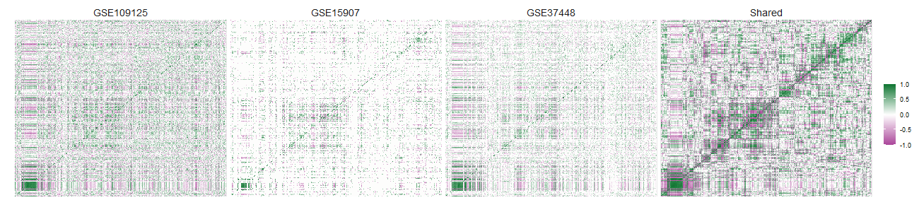
Figure 2: Rescaled study-specific and shared low-rank component for 1000 genes.

Next, we study the correlation induced by the estimated shared covariance matrix $\Lambda\Lambda+\Sigma$. Among the 1000 genes in Figures 1 and 2, we select $209$ “hub” genes that have absolute correlations greater then $0.5$ with at least 10 other genes. Focusing on these hub genes, we show the dependence network in Figure 3, where the size of each gene (i.e. node) is proportional to the number of connections. We identify four main clusters of genes using Louvain method (Clauset et al. 2004). The first one (showed in green) contains genes associated with the immune system such as LAPTM4b (Huygens et al. 2015), CD7 (Aandahl et al. 2003), CD24A (Panagiotou et al. 2022), CD48 (McArdel et al. 2016), and CD55 (Dho et al. 2018). The second cluster (violet) contains many genes important for cancer prognosis, e.g. Prf1 (Guan et al. 2024), Serpinb6b (Al-Khatib et al. 2024), and Ramp1 (Xie et al. 2023). Similar clusters were also found by Hansen et al. (2024) on different datasets. In the third cluster (blue), we observe genes involved in cell growth and proliferation such as Rac2 (Dumont et al. 2009), Stat1 (Chin et al. 1996), and Zbtb20 (Nagao et al. 2016). Finally, the fourth cluster (orange) contains genes Tagap and Atf6 that have been both linked to diabetes (Arshad et al. 2018, Chu et al. 2007).

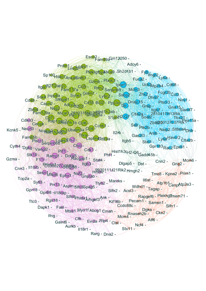
Figure 3: Common gene co-expression network obtained using GEPHI (Bastian et al. 2009) among 209 genes. Nodes (edges) represent genes (positive dependecies). Node size is proportional to the node degree. Node are divided into four main clusters based on their connections.

References

• (1)
• Aach et al. (2000) Aach, J. D., Rindone, W. P. & Church, G. M. (2000), ‘Systematic management and analysis of yeast gene expression data.’, Genome Research 10 4, 431–45.
• Aandahl et al. (2003) Aandahl, E. M., Sandberg, J. K., Beckerman, K. P., Taskén, K., Moretto, W. J. & Nixon, D. F. (2003), ‘CD7 is a differentiation marker that identifies multiple CD8 T cell effector subsets’, The Journal of Immunology 170(5), 2349–2355.
• Al-Khatib et al. (2024) Al-Khatib, S. M., Al-Bzour, A. N., Al-Majali, M. N., Sa’d, L. M., Alramadneh, J. A., Othman, N. R., Al-Mistarehi, A.-H. & Alomari, S. (2024), ‘Exploring Genetic Determinants: A Comprehensive Analysis of Serpin B Family SNPs and Prognosis in Glioblastoma Multiforme Patients’, Cancers 16(6).
• Anceschi et al. (2024) Anceschi, N., Ferrari, F., Dunson, D. B. & Mallick, H. (2024), ‘Bayesian Joint Additive Factor Models for Multiview Learning’, arXiv preprint arXiv:2406.00778 .
• Argelaguet et al. (2020) Argelaguet, R., Arnol, D., Bredikhin, D., Deloro, Y., Velten, B., Marioni, J. & Stegle, O. (2020), ‘MOFA+: A statistical framework for comprehensive integration of multi-modal single-cell data’, Genome Biology 21, 1–17.
• Argelaguet et al. (2018) Argelaguet, R., Velten, B., Arnol, D., Dietrich, S., Zenz, T., Marioni, J. C., Buettner, F., Huber, W. & Stegle, O. (2018), ‘Multi‐Omics Factor Analysis—a framework for unsupervised integration of multi‐omics data sets’, Molecular Systems Biology 14(6), e8124.
• Arshad et al. (2018) Arshad, M., Bhatti, A., John, P., Jalil, F., Borghese, F., Kawalkowska, J. Z., Williams, R. O. & Clanchy, F. I. (2018), ‘T cell activation Rho GTPase activating protein (TAGAP) is upregulated in clinical and experimental arthritis’, Cytokine 104, 130–135.
• Avalos-Pacheco et al. (2022) Avalos-Pacheco, A., Rossell, D. & Savage, R. S. (2022), ‘Heterogeneous Large Datasets Integration Using Bayesian Factor Regression’, Bayesian Analysis 17(1), 33 – 66.
• Bandeira & van Handel (2016) Bandeira, A. S. & van Handel, R. (2016), ‘Sharp nonasymptotic bounds on the norm of random matrices with independent entries’, The Annals of Probability 44(4), 2479 – 2506.
• Bastian et al. (2009) Bastian, M., Heymann, S. & Jacomy, M. (2009), ‘Gephi: An Open Source Software for Exploring and Manipulating Networks’, Proceedings of the International AAAI Conference on Web and Social Media 3(1), 361–362.
• Billingsley (1968) Billingsley, P. (1968), Convergence of Probability Measures, Wiley Series in Probability and Mathematical Statistics, Wiley.
• Boik (2002) Boik, R. J. (2002), ‘Spectral Models for Covariance Matrices’, Biometrika 89(1), 159–182.
• Bortolato & Canale (2024) Bortolato, E. & Canale, A. (2024), ‘Adaptive partition factor analysis’, arXiv preprint arXiv:2410.18939 .
• Boucheron et al. (2013) Boucheron, S., Lugosi, G. & Massart, P. (2013), Concentration Inequalities: A Nonasymptotic Theory of Independence, Oxford University Press.
• Bryan & Hoff (2021) Bryan, J. G. & Hoff, P. D. (2021), ‘Smaller p-values in genomics studies using distilled auxiliary information’, Biostatistics 24(1), 193–208.
• Chandra et al. (2024) Chandra, N. K., Dunson, D. B. & Xu, J. (2024), ‘Inferring Covariance Structure from Multiple Data Sources via Subspace Factor Analysis’, Journal of the American Statistical Association 0(ja), 1–25.