Alternative set-theoretical algorithms for efficient
computations of cliques in Vietoris-Rips complexes

Abstract

Identifying cliques in dense networks remains a formidable challenge, even with significant advances in computational power and methodologies. To tackle this, numerous algorithms have been developed to optimize time and memory usage, implemented across diverse programming languages. Yet, the inherent NP-completeness of the problem continues to hinder performance on large-scale networks, often resulting in memory leaks and slow computations. In the present study, we critically evaluate classic algorithms to pinpoint computational bottlenecks and introduce novel set-theoretical approaches tailored for network clique computation. Our proposed algorithms are rigorously implemented and benchmarked against existing Python-based solutions, demonstrating superior performance. These findings underscore the potential of set-theoretical techniques to drive substantial performance gains in network analysis.

1 Introduction

Network science [44] has emerged as a field providing a powerful framework of tools and methodologies to study complex networks. Its applications and importance span multiple real-world domains, to name a few (but not exclusive), community detection in random graphs [8], social networks [27], protein-protein interactions [40], the detection of co-authorship collaboration networks [39], and economic indicators [51]. One critical aim in the analysis of complex networks is that of identifying cliques, which is known for its NP-hard complexity [28, 7]. In classical algorithms, a typical strategy in identifying cliques is to build upon lower dimensional cliques, such as triangle cliques formed by a combination of edges  [14, 1]. More contemporary algorithms also compute higher-order cliques (i.e. cliques mediated by structures beyond pairwise interactions). These can be used to determine maximal cliques [11, 54, 14, 52, 24] and cliques of all dimensions [59, 53]. However, the most prominent use of higher-order cliques is via recent developments in topological data analysis (TDA)[41, 63]. In this context, clique computation is performed in the background, and this includes cliques emerging from pairwise weighted graph structures, the so-called clique complexes. This information is then used to compute topological invariants, such as, Betti numbers [31, 22], the barcode diagrams [29, 12], the Euler characteristics [34, 36, 19] and the higher-order Forman-Ricci curvature [17, 18]. The computation of high-dimensional cliques is also fundamental in geometrical approaches, for instance, in geometrical data analysis via discrete Ricci curvatures [26, 10, 46], as well as, when computing Laplacians on networks [37]. These geometrical methods are fundamental across various fields of application, such as neuroscience [48, 13, 49], market fragility detection [47], or epidemiology where geometrical data analysis can be used to identify markers and predict epidemic outbreaks [17, 19]. Numerous algorithms have been proposed to address the computational complexity of finding cliques [28, 14, 52, 50, 59, 7, 4], each varying in terms of implementation feasibility and efficiency. However, many of these algorithms face significant challenges, including excessive runtimes for clique detection and memory leaks that hinder their ability to handle large networks. As a result, these algorithms often fall short of efficiently identifying cliques at scale. Set-theoretical approaches [23, 33, 60, 42] offer valuable alternative theoretical formulations for addressing discrete problems, particularly in the construction of posets [5] and simplicial complexes [58]. For example, our recent work in [18] leveraged these methods to provide novel theoretical derivations for efficiently computing the discrete Forman-Ricci curvature in simplicial complexes. The underlying idea was to utilize node adjacency to map and classify cell neighbourhoods. Building on this foundation, we apply this approach here to identify the cells themselves and explore the performance of the proposed method. Specifically, we initially apply this approach to the simplest case of identifying clique triangles, and then extend it to detect higher-order cliques. Throughout this process, we analyze the bottlenecks and key features of each classic algorithm, ultimately developing alternative methods that combine elements of traditional approaches [52, 53] with the node neighbourhood strategy. More specifically, among the various algorithms for finding triangles [1, 32, 2, 2, 15, 55], we drew inspiration from those that iterate over edges. While these algorithms are effective for detecting low-dimensional cliques, they are limited in scope. For computing higher-order cliques in Vietoris-Rips complexes, the authors of [6] propose a simplified expansion that utilizes the simplicial tree method. However, this approach faces significant memory challenges, especially in dense networks, as the simplicial mapping must be stored. In response, we propose algorithms that integrate both methods, alongside the features of the aforementioned algorithms, and introduce an alternative set-theoretical approach inspired by our recent developments[18]. Finally, we benchmarked our proposed algorithm against the classic methods available in the literature. Remarkably, we not only developed new algorithms for computing cliques but also superseded the performance of existing methods found in the literature. Our findings represent a significant advancement in the computation of higher-order structures within complex networks.

The remainder of this article is organised as follows. In Section 2, we briefly recall the foundational concepts of network theory and the Vietoris-Rips complex. Then, in Section 3, we develop novel algorithms, using a set-theoretical approach, for identifying cliques. Subsequently, in Section 4, we benchmark our algorithms and compare their performance with classic implementations available in the literature. Finally, in Section 5, we present our conclusions and propose future perspectives on this work.

2 Basics of network theory

For the sake of clarity, we first outline the essentials of network theory and the Vietoris-Rips complex. For further details, however, we refer the reader to the standard literature on network theory [57, 9] and the Vietoris-Rips complex [61, 62, 21].

2.1 Undirected graph

An undirected simple graph $G=(V,E)$ is defined by a finite set of nodes (vertices) $V$ and a set of edges $E=\{\{x,y\}\,|\,x,y\in V,x\neq y\}$. Let $x,y\in V$. We say that $y$ is a neighbour of $x$ if the edge $(x,y)\in E$. The neighbourhood of node $x$ is defined by a set of nodes that are connected to $x$ via an edge in $E$, and we denote it by $\pi(x)$. Formally,

$$\pi(x)=\{y\in V\,|\,\{x,y\}\in E\}.$$ (1)

A subgraph of $G$ is a pair $G^{\prime}=(V^{\prime},E^{\prime})$ such that $V^{\prime}\subseteq V$ and $E^{\prime}\subseteq E$, and that for all $\{x,y\}\in E^{\prime}$ we have $x,y\in V^{\prime}$. A complete subgraph in $G$ is a subgraph such that all nodes are connected by an edge. The complete subgraphs with $|V^{\prime}|=d$ nodes are called $d$-cliques (or cliques of dimension $d+1$.) We say that $G$ is weighted when we associate a (positive) function $f:E\rightarrow\mathbb{R}$ to the set of edges, and $w=f(e)$ is the weight of the edge $e$.

2.2 Vietoris-Rips Complex and Cliques

Given $d+1$ nodes in a graph $G$, the $d$-simplex associated with these nodes is the $d$-dimensional polytope that their convex hull forms. Hence, a $0$-simplex is a given node, a $1$-simplex is an edge connecting two nodes, a $2$-simplex is a filed triangle, a $3$-simplex is a filed tetrahedron, and so on. In this context, a face of the $d$-simplex formed by $(d+1)$ nodes of $G$ is any simplex obtained by considering a subset of these nodes. Hence, any $d$-simplex possesses $\binom{d+1}{i+1}$ faces of dimension $i$. When $\sigma^{\prime}$ is a face of $\sigma$ such that $|\sigma^{\prime}|=|\sigma|-1$, $\sigma^{\prime}$ is said to belong to the boundary of $\sigma$, denoted by $\partial(\sigma)$.

A simplicial complex $C$ is a set of simplices endowed with the hereditary property: given an element $\sigma\in C$ if $\sigma^{\prime}$ is a face of $\sigma$, then $\sigma^{\prime}\in C$. If $d$ is the maximum dimension of the simplices in $C$, then $C$ is said to be $d$-dimensional and it is called a simplicial $d$-complex. The underlying graph of $C$ is the graph induced by the $1$-simplices (edges) in $C$, i.e., the graph whose node-set is the set of $0$-simplices and whose edge set is the set of $1$-simplices in $C$. If the maximum dimension of $d$ of $C$ is $0$, then $C$ has only $0$-simplices ($1$-cliques or nodes), the case $d=1$ implies that $C$ has $0$ and $1$-simplices ($2$-cliques or edges), when $d=2$ it has up to $2$-simplices ($3$-cliques or triangles), and so on. Consequently, a $d$-simplex $\sigma$ can be induced by a $(d+1)$-clique made of $\binom{d+1}{2}$ edges. In other words, one can associate a network with a simplicial complex by considering a clique complex: each clique (complete subgraph) of $(d+1)$ vertices in the network is seen as a $d$-simplex of a simplicial complex.

Given a set of vertices $V\subseteq\mathbb{R}^{m}$ then let’s consider, for any $x$ in $V$, the open ball centered in $x$ and of radius $\varepsilon>0$ (cutoff parameter): $B_{\varepsilon}(x)=\{y\in\mathbb{R}^{m}\mid\text{dist}(x,y)\leq\varepsilon\}$, where $\text{dist}(x,y)$ is the Euclidean distance between two points $x,y\in\mathbb{R}^{m}$. Then, a Vietoris-Rips (VR) complex $C$ is defined as a set of simplices whose balls only require pairwise intersection to be non-empty, that is,

$$\sigma=\{x_{i}\}_{i}\in C\iff B_{\varepsilon}(x_{i})\cap B_{\varepsilon}(x_{j})\neq\emptyset,\forall x_{i},x_{j}\in\sigma.$$ (2)

This is equivalent to a clique complex of a graph with $V$ as vertex set in which every edge $(x_{i},x_{j})$ satisfies $d(x_{i},x_{j})\leq 2\varepsilon$.

A finite filtration that constructs a Vietoris-Rips complex generates a nested sequence of subcomplexes

$$\emptyset\subseteq C_{\varepsilon_{0}}\subseteq C_{\varepsilon_{1}}\subseteq\ldots\subseteq C_{\varepsilon_{n}}\subseteq C,$$ (3)

where $\varepsilon_{0}\leq\varepsilon_{1}\leq\ldots\leq\varepsilon_{n}$ and $C_{\varepsilon}=\{\sigma=\{x_{i}\}_{i}\,|\,\text{dist}(x_{i},x_{j})\leq 2\varepsilon,\forall x_{i},x_{j}\in\sigma\}$. This leads to a weighted simplicial complex which is parameterised by the cutoff parameter $\varepsilon\geq 0$. Figure 1 shows examples of cliques of different dimensions. This concept is the key point to define a nested chain of simplicial complexes that evolve according to the edges’ weights.

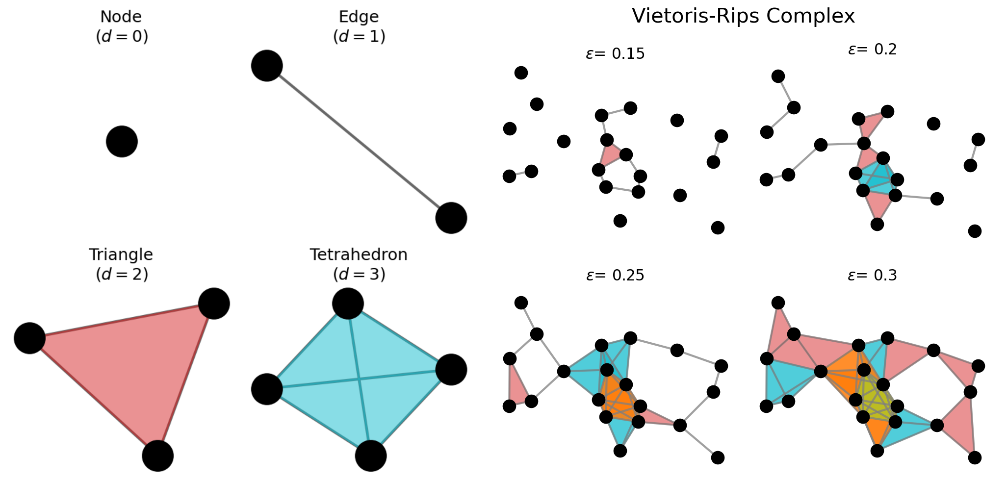
Figure 1: Example of cliques of dimensions $d\in\{0,1,2,3\}$, and the construction of a Vietories-Rips complex for different distance parameters $\varepsilon$. Higher dimensional cliques appear as the cutoff distance increases. For instance, tetrahedron (blue faces), pentahedron (orange faces) and hexahedron (green faces).

3 Proposed Set-theoretical based algorithms

Despite the efficient and natural construction of a Vietoris-Rips complex [62], the process of identifying cliques remains a significant challenge [20, 25]. To address this issue, a wide range of algorithms have been proposed, spanning approaches from computing triangles [14, 50, 32, 2, 15, 55] to the computation of more complex structures [11, 52, 59, 53, 6, 3]. Yet, each algorithm encounters its own set of challenges, such as memory leaks, computation time [11, 59] or difficulties in implementation leading to solutions that are not scalable [35]. To address these issues, we employ set-theoretical approaches [23, 33, 60, 42], which offer alternative optimization strategies for tackling computational problems in computer science. Indeed, it facilitates efficient combinatorial computations and allows us to leverage well-optimized standard libraries for set-theory operations, enabling high-performance implementations. As an example of a recent successful application, we cite our efficient computation of Forman-Ricci curvature of simplicial complexes [17].

To advance, we systematically analyzed state-of-the-art algorithms, identifying both their advantages and critical bottlenecks. This allowed us to pinpoint key features that can be effectively scaled for higher-order cliques. Despite their varying methodologies, most existing algorithms share a fundamental limitation: a static view of node neighbourhoods. This leads to excessive clique searches, redundant data removal, and memory inefficiencies. To address this, we propose novel algorithms that dynamically update node adjacency based on filtration values, enabling efficient processing of evolving networks. Drawing inspiration from the simplicial tree approach, where simplicial paths are stored, we instead maintain local node neighbourhood information as cliques are updated. Our approach, rooted in set-theoretic discretization, builds upon our previous work  [17]. By recursively extending node neighbourhoods to form complete subgraphs, we ensure real-time neighbourhood updates, significantly improving computational efficiency. This dynamic approach not only mitigates memory leaks but also optimizes clique identification, making it highly scalable for complex network structures. The visualization of this extension and its impact on clique detection is explored in detail in Figure 2.

Moreover, a crucial factor for efficiency is identifying cliques at the instant when the neighbourhood is accessed. Building on this principle, we introduce two distinct methods to describe neighbourhood structures:

1. Method 1: Directly from the neighboring nodes of the clique’s boundary;

2. Method 2: Incrementing the node neighbourhood according to the clique’s dimension within the classic node neighbourhood approach.

To implement these methods, we need to define separately the extensions of neighborhood definition for each approach. Method $1$ will be called Dynamic neighbourhood boundary approach and method $2$ will be referred to as Dynamic Multi-layer Node-Neighbourhood approach. In both cases, the starting point for implementation for triangles is described in Algorithm 1; see details in Appendix A.1. For higher-order cliques (dimensions $d_{\max}>2$), the approach will be split between the methods $1$ and $2$, which we explain next.

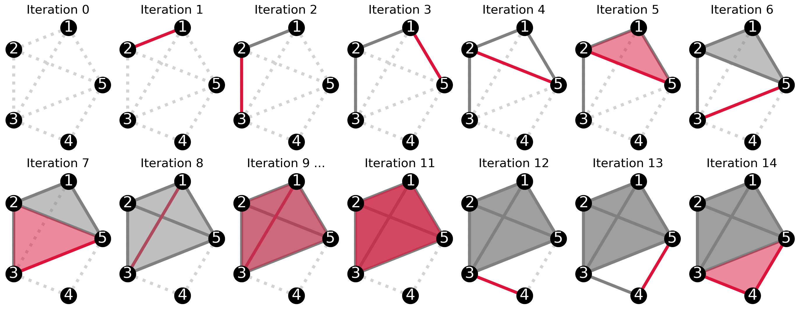
Figure 2: Finding cliques in a simple network as the neighbourhood is updated. The idea of the algorithms relies on the extension of the iterated edges to higher-order simplices. In this case, the ordering of edges is $(1,2),(2,3),(1,5),(3,5),(1,3),(3,4),(4,5)$. One new edge can give rise to several cliques, for instance, edge $(1,3)$ at iteration 8, which provides clique expansions at iterations $9$, $10$ (two triangles - not visible) and $11$ (one tetrahedron).

3.1 Evolving Neighbourhood Boundary Approach

In our previous work [17], we demonstrated that for a $d$-simplex $\sigma$ in a simplicial complex $C$ (with dimension greater than $d$), a $(d+1)$-simplex containing $\sigma$ as a face can be identified using the intersection of the boundary’s neighbourhood in the underlying graph. For instance, if $\sigma$ is a $2$-simplex with vertices $\{x_{1},x_{2},x_{3}\}$, and all these nodes share a common neighbour $x_{4}$ in the graph, then $\{x_{1},x_{2},x_{3},x_{4}\}$ naturally forms a $3$-simplex in $C$, with $\sigma$ as one of its four faces.

Following this idea, we expand the neighbourhood of cliques based on how their boundaries behave, that is, by studying the neighbourhood of each boundary. This information is stored dynamically as the network evolves at each step of edge iteration. As an example, for identifying tetrahedra, we need the information of the previous sequence that generated the triangles, that is, we need the information of the previous triangles as the starting point so that the subsequent list of tetrahedra can be found from the neighbourhood intersection. The same idea underpins the forward method [50], where the triangles are found as an extension of edge iterations.

The optimization challenge lies in providing extensions while avoiding repetitions and storing redundant information. To this end, we update the neighbourhood of the clique boundaries rather than dealing with the neighbourhood of nodes as in the initial approach. More precisely, let $\triangle=\{x,y,z\}$ be a triangle provided by a clique extension, that is, $\triangle=\{x,y\}\cup\{z\}$, where $\{x,y\}$ was the original edge iterated and $z$ is the node that extends the edge to the triangle. For each element $e\in\triangle$, we update the neighbourhood of tetrahedra boundaries, $\pi_{\mathrel{\vbox{\hbox{ \leavevmode\hbox to6.66pt{\vbox to5.82pt{\text{[drawing]}}}}}}}(e):=\pi_{\mathrel{\vbox{\hbox{ \leavevmode\hbox to6.66pt{\vbox to5.82pt{\text{[drawing]}}}}}}}(e)\cup\{\triangle\setminus e\}$, and then we iterate the intersection of the triangles boundaries for finding the tetrahedrons that extend $\triangle$. This idea is formalised in Algorithm 2. Subsequently, for each tetrahedron $\mathrel{\vbox{\hbox{ \leavevmode\hbox to6.66pt{\vbox to5.82pt{\text{[drawing]}}}}}}$, the extension for identifying pentahedra follows the same strategy for updating the neighbourhood and finding the set of nodes that allows this extension from the initial tetrahedron. Explicitly, for each $\triangle\in\,\mathrel{\vbox{\hbox{ \leavevmode\hbox to6.66pt{\vbox to5.82pt{\text{[drawing]}}}}}}$, we update $\pi_{4}(\triangle):=\pi_{4}(\triangle)\cup\{\mathrel{\vbox{\hbox{ \leavevmode\hbox to6.66pt{\vbox to5.82pt{\text{[drawing]}}}}}}\setminus\triangle\}$ and iterate each node of the intersection of neighbours per boundary in $\mathrel{\vbox{\hbox{ \leavevmode\hbox to6.66pt{\vbox to5.82pt{\text{[drawing]}}}}}}$, which extends the tetrahedron to pentahedra. Algorithm 3 describes these dynamics. This idea can naturally be extended to hexahedra (see Algorithm 4) and so forth. Then, a systematic extension to cliques up to dimension $d_{\max}$ is achieved via Algorithm 5. To elucidate the core of our algorithmic insight, Table 2 provides the information of cliques found, as well as, the boundary of each clique per iteration step, for the example depicted in Figure 2. Moreover, Table 3 provides the evolution of the set of boundary neighbours per iteration.

3.2 Evolving Multi-Layer Node-Neighbourhood Approach

Here, we adopt a slightly different approach. Specifically, instead of storing information about clique neighbourhoods from their boundary, we map the higher-order cliques’ information based on the neighbouring nodes whose intersection provides the clique extensions to a higher-order clique (as performed in Algorithm 1). However, we split the neighbourhood information according to their dimension, which is provided as layers per dimension of neighbourhood information. Consequently, the neighbourhood is updated separately, hence avoiding clique repetition.

To exemplify, consider the case of identifying tetrahedra $\mathrel{\vbox{\hbox{ \leavevmode\hbox to6.66pt{\vbox to5.82pt{\text{[drawing]}}}}}}$. First assume we are given the algorithmic steps to finding triangles $\triangle=(x,y,z)$ (originally extended from an iterated edge, $e=(x,y)$). Moreover, assume the neighbourhood for triangles is updated according to Algorithm 1. To update the neighbourhood layer for tetrahedra ($\pi_{\mathrel{\vbox{\hbox{ \leavevmode\hbox to6.66pt{\vbox to5.82pt{\text{[drawing]}}}}}}}$) we iterate all the nodes $c\in e$ and update by adding the last element in for generating the triangle, i.e., $\pi_{\mathrel{\vbox{\hbox{ \leavevmode\hbox to6.66pt{\vbox to5.82pt{\text{[drawing]}}}}}}}:=\pi_{\mathrel{\vbox{\hbox{ \leavevmode\hbox to6.66pt{\vbox to5.82pt{\text{[drawing]}}}}}}}\cup\{z\}$. The intersection of all neighbourhood nodes in $\triangle$ within the $\pi_{\mathrel{\vbox{\hbox{ \leavevmode\hbox to6.66pt{\vbox to5.82pt{\text{[drawing]}}}}}}}$ will provide the set of nodes that extends $\triangle$ to a tetrahedron; Algorithm 6 details this process.

The extensions for identifying pentahedron (cliques of dimension $4$) from a given tetrahedron $\mathrel{\vbox{\hbox{ \leavevmode\hbox to6.66pt{\vbox to5.82pt{\text{[drawing]}}}}}}=(x,y,z,w)$, can naturally be achieved by updating the neighbourhood layer for the pentahedron. Specifically, for each node $n\in\triangle$, we refine its neighbourhood by update $\pi_{4}(n):=\pi_{4}(n)\cup\{w\}$. Further, we compute the intersection of $\pi_{4}(n)$ for all $n$ in $\mathrel{\vbox{\hbox{ \leavevmode\hbox to6.66pt{\vbox to5.82pt{\text{[drawing]}}}}}}$ to find all nodes that extend to pentahedra; this corresponds to Algorithm 7. Analogously, we can find extensions for hexahedron, as described in Algorithm 8. In a recurrent way, we can extend this approach to cliques up to dimension $d_{\max}$ as described in Algorithm 9. To further elucidate our algorithmic strategy, we provide in Table 4 the identified cliques in each iteration for the example depicted in Figure 2.

4 Benchmark Report

To evaluate the efficiency of the proposed algorithms, whose pseudocodes are provided in Appendix A.1, we implemented them in Python [56] and compared their performance with two widely used algorithms for finding cliques, namely, NetworkX [30], which uses Zhang’s algorithm [59] and Gudhi [38], which employs the simplicial tree method [6]. Noteworthy, for our test, we adapted the NetworkX code to allow the search for cliques to be restricted by a specified maximum dimension detailed code available at [16]). The benchmarks were performed on a Dell XPS 15-7590 laptop equipped with an Intel Core i7-9750H CPU and 32GB of RAM, running Ubuntu 20.04.4 LTS. The analysis was divided into two categories: applications using synthetic data and those involving point-cloud data.

4.1 Performance in VR-complex filtrations generated from complete graphs

As an initial step in our testing process, we generated complete graphs with node counts ranging from $30$ to $150$ with increments of $10$ between the two bounds. We ran the algorithms under stress conditions with complete (weighted) graphs, where the filtration process runs until the complete graph is obtained. We limited the search for finding cliques to the maximum dimension $d_{\max}=4$ (up to pentahedron). As depicted in Figure 3, the NetworkX algorithm displays the poorest performance in clique identification, primarily due to memory leaks, which is a significant bottleneck. In contrast, the Gudhi’s clique algorithm exhibits a notable improvement for complete weighted graphs with up to $n=10,000$ nodes (i.e., $\binom{n}{2}$ edges). However, beyond this threshold, memory consumption increases sharply, also negatively impacting processing time. Remarkably, our algorithms outperform both in terms of time and memory efficiency, enabling significantly faster computations and broadening the potential for computing cliques in denser networks. This fact demonstrates the efficiency of our proposed algorithm on computing cliques along large cutoff distances in small dense graphs.

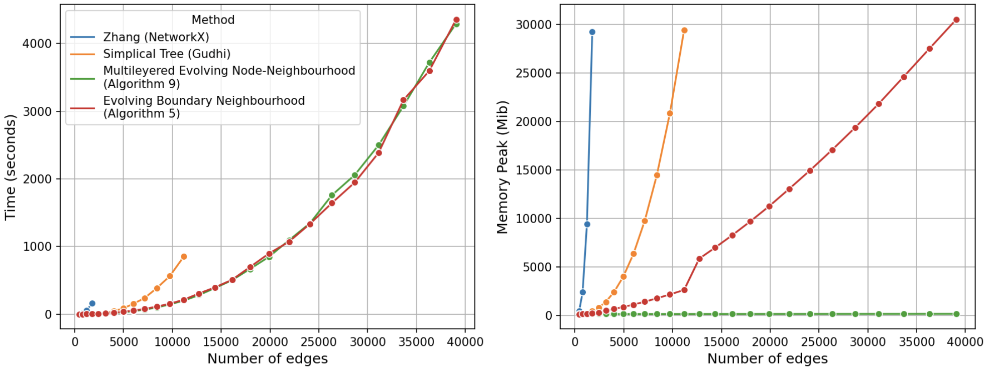
Figure 3: Benchmark comparison between algorithms for finding cliques in VR-complexes from complete networks ($d_{\max}$=4).

4.2 Performance in VR-complexes generated from point cloud data

To evaluate our algorithms using point cloud data, we utilized the files ism_test_horse.pcd and ism_test_cat.pcd, each containing 3,400 nodes (see the Point Cloud Libary repository [43]). For this analysis, we excluded the NetworkX algorithm due to performance issues. We repeated the tests as a function of the cutoff distance between nodes, for the two sets of data and for the clique dimensions $2$ (triangles), $3$ (tetrahedrons), $4$ (pentahedrons), and $5$ (hexahedrons). In all cases, our proposed algorithms outperformed the memory efficiency. The results are shown in Fig. 4 and Fig. 5. Strikingly, the Multilayered Node-Neighbourhood algorithms, particularly Algorithm $9$, demonstrated a significant improvement in preserving neighbourhood information, resulting in the lowest memory leak when compared to the other algorithms analyzed. The drawback of this approach is the inflexibility in choosing the edge ordering, which is required, for instance, in persistence diagram approaches. In contrast, the evolving boundary neighbourhood algorithms (such as Algorithm $5$) allow for the selection of an edge ordering; however, time and memory efficiency are compromised for high-dimensional cliques and higher cutoff values. This is due to the large amount of boundary information that must be stored as the number of cliques increases under these conditions. However, the memory increase is not as significant as with the Gudhi algorithm. Overall, our proposed algorithms can be chosen based on the features required for constructing VR complexes and hardware limitations.

4.3 Performance in unweighted Real-World Networks

To strengthen the performance analysis of our proposed algorithms, we extended the benchmark to unweighted real-world networks. Given Gudhi’s limitation to Vietoris-Rips complexes, we compared our algorithms with a modified version of Zhang’s algorithm (NetworkX). For this, we utilized Facebook data from the SNAP repository [45], with results shown in Figure 6. We evaluated algorithm efficiency based on the maximum clique dimension. Consistent with prior results, our algorithms outperformed others in memory management. Notably, Algorithm 9 achieved the best memory efficiency, ensuring scalability to higher clique dimensions without compromising performance. This advantage arises from storing neighbourhood information per node rather than using Zhang’s method or the boundary storage approach in Algorithm 5. Table 1 summarizes the benchmark, highlighting the strengths and limitations of each method.

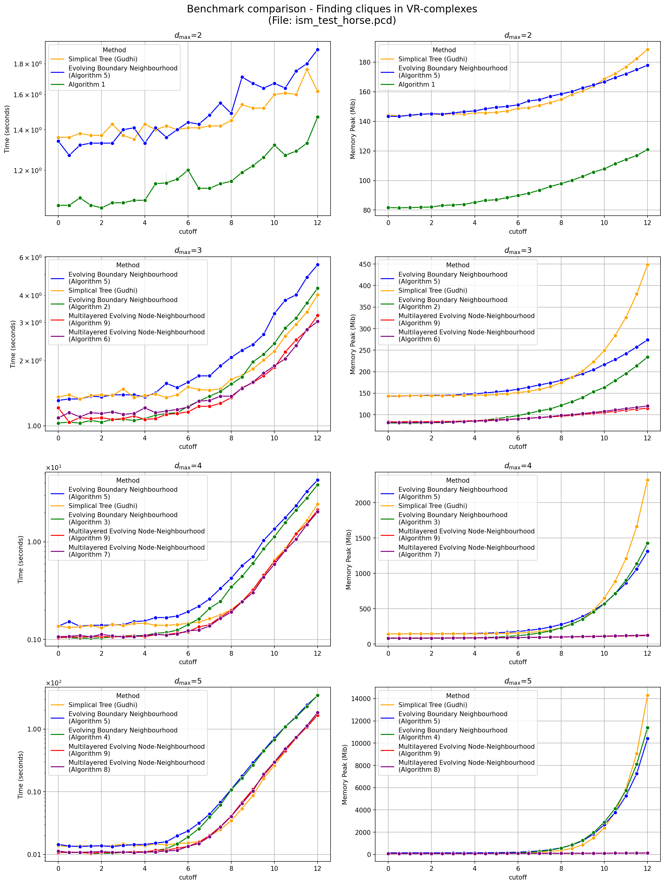
Figure 4: Benchmark comparison between algorithms for finding cliques in VR-complexes from point cloud data ((ism_test_horse.pcd)).

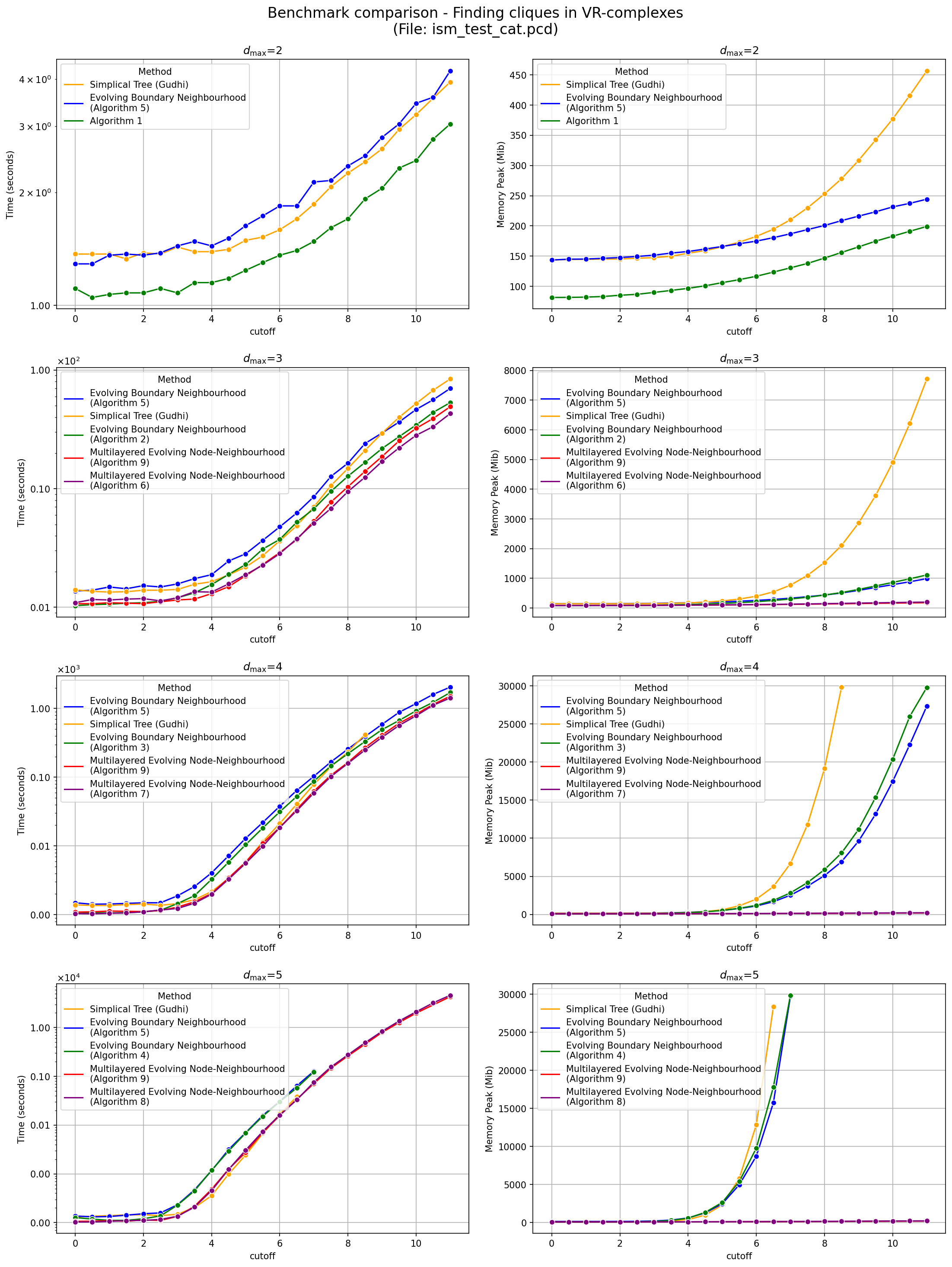
Figure 5: Benchmark comparison between algorithms for finding cliques in VR-complexes from point cloud data ( ism_test_cat.pcd).

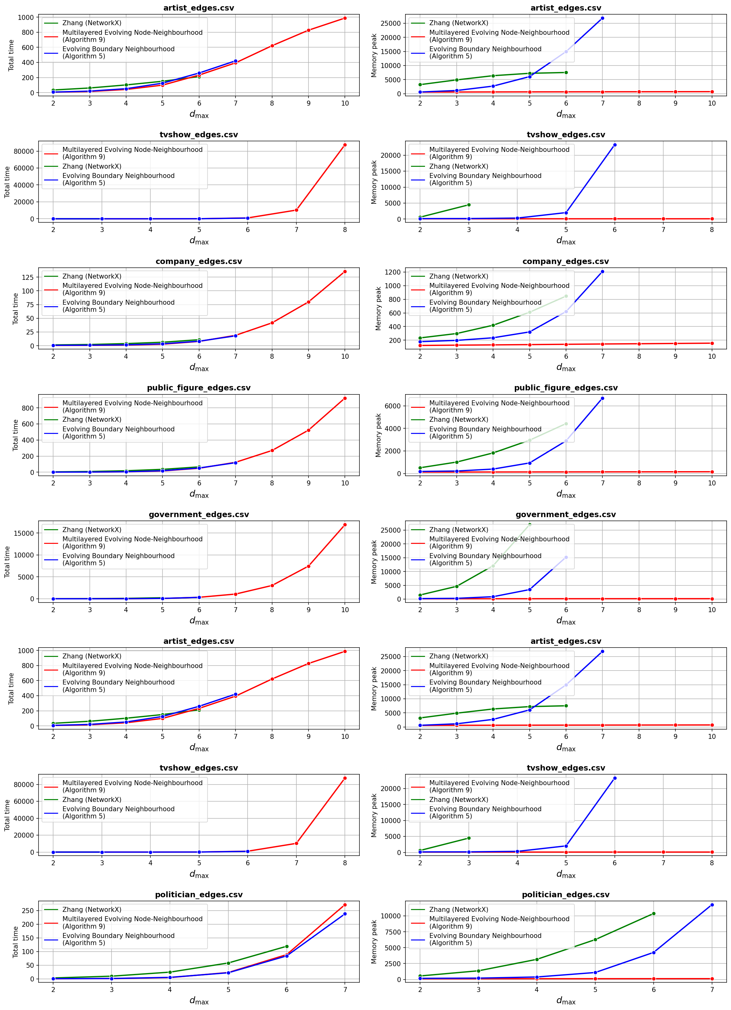
Figure 6: Benchmark comparison between algorithms for finding cliques in VR-complexes from real data unweighted networks (Facebook data from SNAP repository [45]).

Method	Zhang	Simplicial Tree	Neigh. Boundary	Multi-Layered Node-Neighbourhood
Algorithm	NetworkX	Gudhi	Algorithms 2,3,4 and 5	Algorithms 6,7,8 and 9
Memory Efficient	No	No	No	Yes
Sorts Cliques by Weight	No	Yes	No	Yes

Table 1: Summary of the methods bench-marked in our analysis.

5 Conclusion

Network science which includes higher-order networks, is in pursuit of highly efficient algorithms to solve complex challenges across science, engineering, healthcare, and economics. At the core of these networks lies the concept of cliques, a fundamental structure that helps organize the inherent complexity. Yet, the identification of cliques remains an NP-complete problem, presenting a significant computational challenge. To advance, we begin by drawing inspiration from state-of-the-art algorithms for clique identification and analyzing their strengths and limitations. A key drawback of these algorithms is their static view of the node neighbourhood, which induces excessive searching for cliques and redundant information, resulting in inefficient runtime and memory usage. To overcome these challenges, we build on the strengths of our previous work [17], casting these algorithms in the context of set theory. Subsequently, we generalize the identification process to higher-order cliques (specifically cliques within Vietoris-Rips complexes) and improve it by discovering novel ways to explore the neighbourhoods of cliques. In particular, we present two key paradigms, which we denote as evolving neighbourhood boundary and evolving multi-layer node neighbourhood. Further, we leverage well-optimized standard libraries for set-theory operations, enabling Python-based high-performance implementations. Finally, we benchmark and demonstrate that our proposed algorithms provide significant memory efficiency in the context of cliques in dense networks, thus superseding state-of-the-art algorithms. Consequently, we believe that the outcomes of our work will impact big data and complex network science, in particular in the context of topological and geometrical data analysis. For instance, our proposed algorithms can be employed as alternatives for computing the Euler Characteristics and their associated transitions (e.g. via topological phase transitions) in complex systems (e.g. Brain data). Furthermore, the correct choice in the clique’s method computation has the potential use of identifying biological markers (e.g. in personalized medicine) and clustering information from a geometric viewpoint (e.g., by using Forman-Ricci curvature computations.)

Appendix A Pseudo-codes

In this section, we provide the pseudocodes derived from our theoretical and computational analysis and for completeness the classic methods that inspired our work.

A.1 Proposed Algorithms

Algorithm 1 Find Triangles (Evolving Neighborhood Approach)

1:List of edges, $E$

2:$\pi=\emptyset$

3:for $e=(x,y)\in E$  do

4:  $\pi(x):=\pi(x)\cup\{y\}$

5:  $\pi(y):=\pi(y)\cup\{x\}$

6:  $Z=\pi(x)\cap\pi(y)$

7:  for $z\in Z$ do

8:   print $\{x,y,z\}$

9:  end for

10:end for

Algorithm 2 Find Triangles and Tetrahedrons (Evolving Boundary Neighborhood Approach)

1:List of (sorted) edges, $E$

2:$\pi_{\triangle}=\emptyset,\pi_{\mathrel{\vbox{\hbox{ \leavevmode\hbox to6.66pt{\vbox to5.82pt{\text{[drawing]}}}}}}}=\emptyset$

3:for $e=(x,y)\in E$  do

4:  $\pi_{\triangle}(x):=\pi_{\triangle}(x)\cup\{y\}$

5:  $\pi_{\triangle}(y):=\pi_{\triangle}(y)\cup\{x\}$

6:  $Z=\pi_{\triangle}(x)\cap\pi_{\triangle}(y)$

7:  for $z\in Z$ do

8:   $\triangle=\{x,y,z\}$

9:   print $\triangle$

10:   $\partial(\triangle)=\{\{x,y\},\{x,z\},\{y,z\}\}$

11:   $\pi_{\mathrel{\vbox{\hbox{ \leavevmode\hbox to6.66pt{\vbox to5.82pt{\text{[drawing]}}}}}}}(\{x,y\}):=\pi_{\mathrel{\vbox{\hbox{ \leavevmode\hbox to6.66pt{\vbox to5.82pt{\text{[drawing]}}}}}}}(\{x,y\})\cup\{z\}$

12:   $\pi_{\mathrel{\vbox{\hbox{ \leavevmode\hbox to6.66pt{\vbox to5.82pt{\text{[drawing]}}}}}}}(\{x,z\}):=\pi_{\mathrel{\vbox{\hbox{ \leavevmode\hbox to6.66pt{\vbox to5.82pt{\text{[drawing]}}}}}}}(\{x,z\})\cup\{y\}$

13:   $\pi_{\mathrel{\vbox{\hbox{ \leavevmode\hbox to6.66pt{\vbox to5.82pt{\text{[drawing]}}}}}}}(\{y,z\}):=\pi_{\mathrel{\vbox{\hbox{ \leavevmode\hbox to6.66pt{\vbox to5.82pt{\text{[drawing]}}}}}}}(\{y,z\})\cup\{x\}$

14:   $W=\pi_{\mathrel{\vbox{\hbox{ \leavevmode\hbox to6.66pt{\vbox to5.82pt{\text{[drawing]}}}}}}}(\{x,y\})\cap\pi_{\mathrel{\vbox{\hbox{ \leavevmode\hbox to6.66pt{\vbox to5.82pt{\text{[drawing]}}}}}}}(\{x,z\})\cap\pi_{\mathrel{\vbox{\hbox{ \leavevmode\hbox to6.66pt{\vbox to5.82pt{\text{[drawing]}}}}}}}(\{y,z\})$

15:   for $w\in W$ do

16:     $\mathrel{\vbox{\hbox{ \leavevmode\hbox to6.66pt{\vbox to5.82pt{\text{[drawing]}}}}}}=\{x,y,z,w\}$

17:     print $\mathrel{\vbox{\hbox{ \leavevmode\hbox to6.66pt{\vbox to5.82pt{\text{[drawing]}}}}}}$

18:   end for

19:  end for

20:end for

21:

Algorithm 3 Find up to pentahedrons (Evolving Boundary Neighborhood Approach)

1:List of (sorted) edges, $E$

2:$\pi_{2}=\emptyset,\pi_{3}=\emptyset,\pi_{4}=\emptyset$

3:for $e=(x,y)\in E$  do

4:  $\pi_{2}(x):=\pi_{2}(x)\cup\{y\}$

5:  $\pi_{2}(y):=\pi_{2}(y)\cup\{x\}$

6:  $Z=\pi_{2}(x)\cap\pi_{2}(y)$

7:  for $z\in Z$ do

8:   $\tau_{2}=\{x,y,z\}$

9:   print $\tau_{2}$

10:   $\partial(\tau_{2})=\{\{x,y\},\{x,z\},\{y,z\}\}$

11:   $\pi_{3}(\{x,y\}):=\pi_{3}(\{x,y\})\cup\{z\}$

12:   $\pi_{3}(\{x,z\}):=\pi_{3}(\{x,z\})\cup\{y\}$

13:   $\pi_{3}(\{y,z\}):=\pi_{3}(\{y,z\})\cup\{x\}$

14:   $W=\pi_{3}(\{x,y\})\cap\pi_{3}(\{x,z\})\cap\pi_{3}(\{y,z\})$

15:   for $w\in W$ do

16:     $\tau_{3}=\{x,y,z,w\}$

17:     print $\tau_{3}$

18:     $\partial(\tau_{3})=\{\{x,y,z\},\{x,y,w\},\{x,z,w\},\{y,z,w\}\}$

19:     $\pi_{4}(\{x,y,z\}):=\pi_{4}(\{x,y,z\})\cup\{w\}$

20:     $\pi_{4}(\{x,y,w\}):=\pi_{4}(\{x,y,w\})\cup\{z\}$

21:     $\pi_{4}(\{x,z,w\}):=\pi_{4}(\{x,z,w\})\cup\{y\}$

22:     $\pi_{4}(\{y,z,w\}):=\pi_{4}(\{y,z,w\})\cup\{x\}$

23:     $Q=\pi_{4}(\{x,y,z\})\cap\pi_{4}(\{x,y,w\})\cap\pi_{4}(\{x,z,w\})\cap\pi_{4}(\{y,z,w\})$

24:     for $q\in Q$ do

25:      $\tau_{4}=\{x,y,z,w,q\}$

26:      print $\tau_{4}$

27:     end for

28:   end for

29:  end for

30:end for

Algorithm 4 Find up to hexahedrons (Evolving Boundary Neighborhood Approach)

1:List of (sorted) edges, $E$

2:$\pi_{2}=\emptyset,\pi_{3}=\emptyset,\pi_{4}=\emptyset,\pi_{5}=\emptyset$

3:for $e=(x,y)\in E$  do

4:  $\pi_{2}(x):=\pi_{2}(x)\cup\{y\}$

5:  $\pi_{2}(y):=\pi_{2}(y)\cup\{x\}$

6:  $V=\pi_{2}(x)\cap\pi_{2}(y)$

7:  for $z\in Z$ do

8:   $\tau_{2}=\{x,y,z\}$

9:   print $\tau_{2}$

10:   $\partial(\tau_{2})=\{\{x,y\},\{x,z\},\{y,z\}\}$

11:   $\pi_{3}(\{x,y\}):=\pi_{3}(\{x,y\})\cup\{z\}$

12:   $\pi_{3}(\{x,z\}):=\pi_{3}(\{x,z\})\cup\{y\}$

13:   $\pi_{3}(\{y,z\}):=\pi_{3}(\{y,z\})\cup\{x\}$

14:   $W=\pi_{3}(\{x,y\})\cap\pi_{3}(\{x,z\})\cap\pi_{3}(\{y,z\})$

15:   for $w\in W$ do

16:     $\tau_{3}=\{x,y,z,w\}$

17:     print $\tau_{3}$

18:     $\partial(\tau_{3})=\{\{x,y,z\},\{x,y,w\},\{x,z,w\},\{y,z,w\}\}$

19:     $\pi_{4}(\{x,y,z\}):=\pi_{4}(\{x,y,z\})\cup\{w\}$

20:     $\pi_{4}(\{x,y,w\}):=\pi_{4}(\{x,y,w\})\cup\{z\}$

21:     $\pi_{4}(\{x,z,w\}):=\pi_{4}(\{x,z,w\})\cup\{y\}$

22:     $\pi_{4}(\{y,z,w\}):=\pi_{4}(\{y,z,w\})\cup\{x\}$

23:     $Q=\pi_{4}(\{x,y,z\})\cap\pi_{4}(\{x,y,w\})\cap\pi_{4}(\{x,z,w\})\cap\pi_{4}(\{y,z,w\})$

24:     for $q\in Q$ do

25:      $\tau_{4}=\{x,y,z,w,q\}$

26:      print $\tau_{4}$

27:      $\partial(\tau_{4})=\{\{x,y,z,w\},\{x,y,z,q\},\{x,y,w,q\},\{x,z,w,q\},\{y,z,w,q\}\}$

28:      $\pi_{5}(\{x,y,z,w\}):=\pi_{5}(\{x,y,z,w\})\cup\{q\}$

29:      $\pi_{5}(\{x,y,z,q\}):=\pi_{5}(\{x,y,z,q\})\cup\{w\}$

30:      $\pi_{5}(\{x,y,w,q\}):=\pi_{5}(\{x,y,w,q\})\cup\{z\}$

31:      $\pi_{5}(\{x,z,w,q\}):=\pi_{5}(\{x,z,w,q\})\cup\{y\}$

32:      $\pi_{5}(\{y,z,w,q\}):=\pi_{5}(\{y,z,w,q\})\cup\{x\}$

33:      $R=\pi_{5}(\{x,y,z,w\})\cap\pi_{5}(\{x,y,z,q\})\cap\pi_{5}(\{x,y,w,q\})\cap\pi_{5}(\{x,z,w,q\})\cap\pi_{5}(\{y,z,w,q\})$

34:      for $r\in R$ do

35:        $\tau_{5}=\{x,y,z,w,q,r\}$

36:        print $\tau_{5}$

37:      end for

38:     end for

39:   end for

40:  end for

41:end for

Algorithm 5 Compute Cliques (Recursive Evolving Boundary Neighbourhood Approach)

1:procedure ComputeCliques($E$,$d_{\max}$)

2:  Input: $E$, the list of (sorted) edge, $d_{\max}$, the maximum clique dimension

3:  Output: All the cliques up to dimension $d_{\max}$

4:  Initialization:

5:  $\pi_{d}=\emptyset,\,\forall d\in\{2,\ldots,d_{\max}\}$

6:

7:  procedure AuxiliaryFunction($\sigma$)

8:   Input: $\sigma$, a clique

9:   Output: A sequence of cliques $\tau$ extended from $\sigma$

10:   $d=|\sigma|$

11:   print $\sigma$

12:   

13:   if $d<d_{\max}$ then

14:     for $\gamma\in\partial(\sigma)$ do

15:      $\pi_{d}(\gamma):=\pi_{d}(\gamma)\cup\{\sigma\setminus\gamma\}$

16:     end for

17:     $Z=\cap_{\gamma\in\partial(\sigma)}\pi_{d}(\gamma)$

18:     for $z\in Z$ do

19:      $\tau=\sigma\cup\{z\}$

20:      compute AuxiliaryFunction($\tau$)

21:     end for

22:   end if

23:  end procedure

24:  

25:  for $e\in E$ do

26:   compute AuxiliaryFuncion(e)

27:  end for

28:  

29:end procedure

A.2 Evolving Multilayered Node-Neighbourhood Algorithms

Algorithm 6 Find Triangles and Tetrahedrons (Evolving Multilayered Node-Neighborhood Approach)

1:List of edges (sorted in lexicographic order), $E$

2:$\pi_{\triangle}=\emptyset,\pi_{\mathrel{\vbox{\hbox{ \leavevmode\hbox to6.66pt{\vbox to5.82pt{\text{[drawing]}}}}}}}=\emptyset$

3:for $e=(x,y)\in E$  do

4:  $\pi_{\triangle}(x):=\pi_{\triangle}(x)\cup\{y\}$

5:  $\pi_{\triangle}(y):=\pi_{\triangle}(y)\cup\{x\}$

6:  $Z=\pi_{\triangle}(x)\cap\pi_{\triangle}(y)$

7:  for $z\in Z$ do

8:   $\triangle=\{x,y,z\}$

9:   print $\triangle$

10:   for $c\in e$ do

11:     $\pi_{\mathrel{\vbox{\hbox{ \leavevmode\hbox to6.66pt{\vbox to5.82pt{\text{[drawing]}}}}}}}(c):=\pi_{\mathrel{\vbox{\hbox{ \leavevmode\hbox to6.66pt{\vbox to5.82pt{\text{[drawing]}}}}}}}(c)\cup\{z\}$

12:   end for

13:   $W=\pi_{\mathrel{\vbox{\hbox{ \leavevmode\hbox to6.66pt{\vbox to5.82pt{\text{[drawing]}}}}}}}(x)\cap\pi_{\mathrel{\vbox{\hbox{ \leavevmode\hbox to6.66pt{\vbox to5.82pt{\text{[drawing]}}}}}}}(y)\cap\pi_{\mathrel{\vbox{\hbox{ \leavevmode\hbox to6.66pt{\vbox to5.82pt{\text{[drawing]}}}}}}}(z)$

14:   for $w\in W$ do

15:     $\mathrel{\vbox{\hbox{ \leavevmode\hbox to6.66pt{\vbox to5.82pt{\text{[drawing]}}}}}}=\{x,y,z,w\}$

16:     print $\mathrel{\vbox{\hbox{ \leavevmode\hbox to6.66pt{\vbox to5.82pt{\text{[drawing]}}}}}}$

17:   end for

18:  end for

19:end for

Algorithm 7 Find up to Pentahedrons (Evolving Multilayered Node-Neighborhood Approach)

1:List of edges (sorted in lexicographic order), $E$

2:$\pi_{2}=\emptyset,\pi_{3}=\emptyset,\pi_{4}=\emptyset$

3:for $e=(x,y)\in E$  do

4:  $\pi_{2}(x):=\pi_{2}(x)\cup\{y\}$

5:  $\pi_{2}(y):=\pi_{2}(y)\cup\{x\}$

6:  $Z=\pi_{2}(x)\cap\pi_{2}(y)$

7:  for $z\in Z$ do

8:   $\tau_{2}=\{x,y,z\}$

9:   print $\tau_{2}$

10:   for $n\in e$ do

11:     $\pi_{3}(n):=\pi_{3}(n)\cup\{z\}$

12:   end for

13:   $W=\pi_{3}(x)\cap\pi_{3}(y)\cap\pi_{3}(z)$

14:   for $w\in W$ do

15:     $\tau_{4}=\{x,y,z,w\}$

16:     print $\tau_{3}$

17:     for $n\in\tau_{2}$ do

18:      $\pi_{4}(n):=\pi_{4}(n)\cup\{w\}$

19:     end for

20:     $Q=\pi_{4}(x)\cap\pi_{4}(y)\cap\pi_{4}(z)\cap\pi_{4}(w)$

21:     for $q\in Q$ do

22:      $\tau_{4}=\{x,y,z,w,q\}$

23:      print $\tau_{4}$

24:     end for

25:   end for

26:  end for

27:end for

Algorithm 8 Find up to Hexahedrons (Evolving Multilayered Node-Neighborhood Approach)

1:List of edges (sorted in lexicographic order), $E$

2:$\pi_{2}=\emptyset,\pi_{3}=\emptyset,\pi_{4}=\emptyset,\pi_{5}=\emptyset$

3:for $e=(x,y)\in E$  do

4:  $\pi_{2}(x):=\pi_{2}(x)\cup\{y\}$

5:  $\pi_{2}(y):=\pi_{2}(y)\cup\{x\}$

6:  $Z=\pi_{2}(x)\cap\pi_{2}(y)$

7:  for $z\in Z$ do

8:   $\tau_{2}=\{x,y,z\}$

9:   print $\tau_{2}$

10:   for $n\in e$ do

11:     $\pi_{3}(n):=\pi_{3}(n)\cup(\{z\}$

12:   end for

13:   $W=\pi_{3}(x)\cap\pi_{3}(y)\cap\pi_{3}(z)$

14:   for $w\in W$ do

15:     $\tau_{4}=\{x,y,z,w\}$

16:     print $\tau_{3}$

17:     for $n\in\tau_{2}$ do

18:      $\pi_{4}(n):=\pi_{4}(n)\cup(\{w\}$

19:     end for

20:     $Q=\pi_{4}(x)\cap\pi_{4}(y)\cap\pi_{4}(z)\cap\pi_{4}(w)$

21:     for $q\in Q$ do

22:      $\tau_{4}=\{x,y,z,w,q\}$

23:      print $\tau_{4}$

24:     end for

25:     for $n\in\tau_{3}$ do

26:      $\pi_{5}(n):=\pi_{4}(n)\cup\{q\}$

27:     end for

28:     $R=\pi_{5}(x)\cap\pi_{5}(y)\cap\pi_{5}(z)\cap\pi_{5}(w)\cap\pi_{5}(q)$

29:     for $r\in R$ do

30:      $\tau_{5}=\{x,z,y,w,q,r\}$

31:      print $\tau_{5}$

32:     end for

33:   end for

34:  end for

35:end for

Algorithm 9 Compute Cliques (Recursive Evolving Dynamic Multilayered Node-Neighbourhood Approach)

1:procedure ComputeCliques($E$,$d_{\max}$)

2:  Input: $E$, the list of (sorted) edges, $d_{\max}$, the maximum clique dimension

3:  Output: All the cliques up to dimension $d_{\max}$

4:  Initialization:

5:  $\pi_{d}=\emptyset,\,\forall d\in\{2,\ldots,d_{\max}\}$

6:

7:  procedure AuxiliaryFunction($\sigma$)

8:   Input: $\sigma=(x_{0},x_{1},\ldots,x_{\dim})$, a clique described as an ascending sequence of nodes

9:   Output: A sequence of cliques $\tau$ extended from $\sigma$

10:   $d=|\sigma|$

11:   print $\sigma$

12:   $\hat{\sigma}:=\sigma\setminus\{x_{\dim}\}$

13:   

14:   if $d<d_{\max}$ then

15:     if $d>2$ then

16:      for  $n\in\hat{\sigma}$ do

17:        $\pi_{d}(x):=\pi_{d}(n)\cup\{x_{\dim}\}$

18:      end for

19:     else

20:      $\sigma=\{x,y\}$

21:      $\pi_{2}(x):=\pi_{2}(x)\cup\{y\}$

22:      $\pi_{2}(y):=\pi_{2}(y)\cup\{x\}$

23:     end if

24:     $Z=\cap_{n\in\sigma}\pi_{d}(n)$

25:     for $z\in Z$ do

26:      $\tau=\sigma\cup\{z\}$

27:      compute AuxiliaryFunction($\tau$)

28:     end for

29:   end if

30:  end procedure

31:  

32:  for $e\in E$ do

33:   compute AuxiliaryFuncion(e)

34:  end for

35:  

36:end procedure

A.3 Classic Algorithms

The K3 algorithm was developed in [14]; the forward method in [50].

Algorithm 10 Find Triangles (Edge-Iterator)

1:$E$, the List of edges; $\pi$, the node neighbourhood

2:for $e=(x,y)\in E$  do

3:  $Z=\pi(x)\cap\pi(y)$

4:  for $z\in Z$ do

5:   print $(x,y,v)$

6:  end for

7:end for

Algorithm 11 Find Triangles (K3 Method)

1:$G=(V,E)$, an undirected simple graph

2:Sorted sequence of nodes ($V=(v_{1},v_{2},\ldots,v_{n})$) in descending order of degree

3:Create the set of marked nodes, $M=\emptyset$

4:for $i\in(1,2,\ldots,n-2)$ do

5:  $M:=M\cup\pi(v_{i})$

6:  for $u\in M$ do

7:   for $w\in\pi(u)$ do

8:     if $w\in M$ then print $\{v_{i},u,w\}$

9:      $M:=M\setminus\{u\}$

10:     end if

11:   end for

12:  end for

13:  $V:=V\setminus\{v_{i}\}$

14:end for

Algorithm 12 Find Triangles (forward method)

1:$V$, the list of nodes (ordered by node degree in decreasing order); $\pi$ the adjacency of nodes

2:$A(x):=\emptyset,\,\forall v\in V$

3:for $y\in V$ do

4:  for $z\in\pi(y)$ do

5:   if $y<z$ then

6:     for $x\in A(y)\cap A(z)$ do

7:      print $\{x,y,z\}$

8:     end for

9:     $A(z):=A(z)\cup\{y\}$

10:   end if

11:  end for

12:end for

Appendix B Tables

In this section, we provide the tables to elucidate the iteration process or our algorithms. We used the Figure 2 to provide the examples. We also provide the cliques counting from the benchmark performed in Section 4.

Iteration	Clique Found	Boundary of Clique
0	$\emptyset$	-
1	$\{1,2\}$	$\{\{1\},\{2\}\}$
2	$\{2,3\}$	$\{\{2\},\{3\}\}$
3	$\{1,5\}$	$\{\{1\},\{5\}\}$
4	$\{2,5\}$	$\{\{2\},\{5\}\}$
5	$\{1,2,5\}$	$\{\{2,5\},\{1,2\},\{1,5\}\}$
6	$\{3,5\}$	$\{\{3\},\{5\}\}$
7	$\{2,3,5\}$	$\{\{3,5\},\{2,3\},\{2,5\}\}$
8	$\{1,3\}$	$\{\{1\},\{3\}\}$
9	$\{1,2,3\}$	$\{\{1,3\},\{1,2\},\{2,3\}\}$
10	$\{1,3,5\}$	$\{\{1,3\},\{1,5\},\{3,5\}\}$
11	$\{1,2,3\}$	$\{\{1,3\},\{1,2\},\{2,3\}\}$
12	$\{3,4\}$	$\{\{3\},\{4\}\}$
13	$\{4,5\}$	$\{\{5\},\{4\}\}$
14	$\{3,4,5\}$	$\{\{4,5\},\{3,5\},\{3,4\}\}$

Table 2: The evolution of the cliques finding and the description of the boundary of each clique found in the iteration process of the Algorithm 5 on Figure 2.

Iteration	Updated Boundary Set
0	N/A
1	$\{1\}:\{2\},\{2\}:\{1\}$
2	$\{1\}:\{2\},\{2\}:\{1,3\},\{3\}:\{2\}$
3	$\{1\}:\{2,5\},\{2\}:\{1,3\},\{3\}:\{2\},\{5\}:\{1\}$
4	$\{1\}:\{2,5\},\{2\}:\{1,3,5\},\{3\}:\{2\},\{5\}:\{1,2\}$
5	$\{1\}:\{2,5\},\{2\}:\{1,3,5\},\{3\}:\{2\},\{5\}:\{1,2\},\{2,5\}:\{1\},\{1,2\}:\{5\},\{1,5\}:\{2\}$
6	$\{1\}:\{2,5\},\{2\}:\{1,3,5\},\{3\}:\{2,5\},\{5\}:\{1,2,3\},\{2,5\}:\{1\},\{1,2\}:\{5\},\{1,5\}:\{2\}$
7	$\{1\}:\{2,5\},\{2\}:\{1,3,5\},\{3\}:\{2,5\},\{5\}:\{1,2,3\},\{2,5\}:\{1,3\},\{1,2\}:\{5\},\{1,5\}:\{2\},\{3,5\}:\{2\},\{2,3\}:\{5\}$
8	$\{1\}:\{2,3,5\},\{2\}:\{1,3,5\},\{3\}:\{1,2,5\},\{5\}:\{1,2,3\},\{2,5\}:\{1,3\},\{1,2\}:\{5\},\{1,5\}:\{2\},\{3,5\}:\{2\},\{2,3\}:\{1,5\}$
9	$\{1\}:\{2,3,5\},\{2\}:\{1,3,5\},\{3\}:\{1,2,5\},\{5\}:\{1,2,3\},\{2,5\}:\{1,3\},\{1,2\}:\{3,5\},\{1,5\}:\{2\},\{3,5\}:\{2\},\{2,3\}:\{1,5\},\{1,3\}:\{2\}$
10	$\{1\}:\{2,3,5\},\{2\}:\{1,3,5\},\{3\}:\{1,2,5\},\{5\}:\{1,2,3\},\{2,5\}:\{1,3\},\{1,2\}:\{3,5\},\{1,5\}:\{2,3\},\{3,5\}:\{1,2\},\{2,3\}:\{1,5\},\{1,3\}:\{2,5\}$
11	$\{1\}:\{2,3,5\},\{2\}:\{1,3,5\},\{3\}:\{1,2,5\},\{5\}:\{1,2,3\},\{2,5\}:\{1,3\},\{1,2\}:\{3,5\},\{1,5\}:\{2,3\},\{3,5\}:\{1,2\},\{2,3\}:\{1,5\},\{1,3\}:\{2,5\},\{1,2,3,5\}$
12	$\{1\}:\{2,3,5\},\{2\}:\{1,3,5\},\{3\}:\{1,2,4,5\},\{5\}:\{1,2,3,4\},\{2,5\}:\{1,3\},\{1,2\}:\{3,5\},\{1,5\}:\{2,3\},\{3,5\}:\{1,2\},\{2,3\}:\{1,5\},\{4\}:\{3\}$
13	$\{1\}:\{2,3,5\},\{2\}:\{1,3,5\},\{3\}:\{1,2,4,5\},\{5\}:\{1,2,3,4\},\{2,5\}:\{1,3\},\{1,2\}:\{3,5\},\{1,5\}:\{2,3\},\{3,5\}:\{1,2\},\{2,3\}:\{1,5\},\{4\}:\{3,5\},\{4,5\}:\{3\}$
14	$\{1\}:\{2,3,5\},\{2\}:\{1,3,5\},\{3\}:\{1,2,4,5\},\{5\}:\{1,2,3,4\},\{2,5\}:\{1,3\},\{1,2\}:\{3,5\},\{1,5\}:\{2,3\},\{3,5\}:\{1,2\},\{2,3\}:\{1,5\},\{4\}:\{3,5\},\{4,5\}:\{3\},\{3,4\}:\{5\}$

Table 3: The evolution of the boundary neighbourhood of the graph in Figure 2 by using the Algorithm 9.

Iteration	Current Neighborhood Updates	Clique Found
0	$\pi_{2}$: {1: {}, 2: {}, 3: {}, 5: {}, 4: {}}, $\pi_{3}$: {1: {}, 2: {}, 3: {}, 5: {}, 4: {}}	-
1	$\pi_{2}(1):=\pi_{2}(1)\cup\{2\}=\{2\},\pi_{2}(2):=\pi_{2}(2)\cup\{1\}=\{1\}$	{1, 2}
2	$\pi_{2}(1):=\pi_{2}(1)\cup\{5\}=\{2,5\},\pi_{2}(5):=\pi_{2}(5)\cup\{1\}=\{1\}$	{1, 5}
3	$\pi_{2}(1):=\pi_{2}(1)\cup\{3\}=\{2,3,5\},\pi_{2}(3):=\pi_{2}(3)\cup\{1\}=\{1\}$	{1, 3}
4	$\pi_{2}(2):=\pi_{2}(2)\cup\{3\}=\{1,3\},\pi_{2}(3):=\pi_{2}(3)\cup\{2\}=\{1,2\}$	{2, 3}
5	$\pi_{3}(2):=\pi_{3}(2)\cup(\pi_{3}(2)-\{2,3\})=\{1\},\pi_{3}(3):=\pi_{3}(3)\cup(\pi_{3}(3)-\{2,3\})=\{1\}$	{1, 2, 3}
6	$\pi_{2}(2):=\pi_{2}(2)\cup\{5\}=\{1,3,5\},\pi_{2}(5):=\pi_{2}(5)\cup\{2\}=\{1,2\}$	{2, 5}
7	$\pi_{3}(2):=\pi_{3}(2)\cup(\pi_{3}(2)-\{2,5\})=\{1\},\pi_{3}(5):=\pi_{3}(5)\cup(\pi_{3}(5)-\{2,5\})=\{1\}$	{1, 2, 5}
8	$\pi_{2}(3):=\pi_{2}(3)\cup\{5\}=\{1,2,5\},\pi_{2}(5):=\pi_{2}(5)\cup\{3\}=\{1,2,3\}$	{3, 5}
9	$\pi_{3}(3):=\pi_{3}(3)\cup(\pi_{3}(3)-\{3,5\})=\{1\},\pi_{3}(5):=\pi_{3}(5)\cup(\pi_{3}(5)-\{3,5\})=\{1\}$	{1, 3, 5}
10	$\pi_{3}(3):=\pi_{3}(3)\cup(\pi_{3}(3)-\{3,5\})=\{1,2\},\pi_{3}(5):=\pi_{3}(5)\cup(\pi_{3}(5)-\{3,5\})=\{1,2\}$	{2, 3, 5}
11	No neighborhood updates.	{1, 2, 3, 5}
12	$\pi_{2}(3):=\pi_{2}(3)\cup\{4\}=\{1,2,4,5\},\pi_{2}(4):=\pi_{2}(4)\cup\{3\}=\{3\}$	{3, 4}
13	$\pi_{2}(5):=\pi_{2}(5)\cup\{4\}=\{1,2,3,4\},\pi_{2}(4):=\pi_{2}(4)\cup\{5\}=\{3,5\}$	{4, 5}
14	$\pi_{3}(5):=\pi_{3}(5)\cup(\pi_{3}(5)-\{4,5\})=\{1,2,3\},\pi_{3}(4):=\pi_{3}(4)\cup(\pi_{3}(4)-\{4,5\})=\{3\}$	{3, 4, 5}

Table 4: The evolution of the cliques search in the example of Figure 2 by using the Evolving Dynamic Multilayered Node-Neighbourhood Approach (Algorithm 9).

	Method	$d_{\max}$	Number of nodes	Number of edges	Number of cliques
0	NetworkX	2	50515	819090	3143305
1	Algorithm 9	2	50515	819090	3143305
2	Algorithm 5	2	50515	819090	3143305
3	NetworkX	3	50515	819090	7613489
4	Algorithm 9	3	50515	819090	7613489
5	Algorithm 5	3	50515	819090	7613489
6	NetworkX	4	50515	819090	14757799
7	Algorithm 9	4	50515	819090	14757799
8	Algorithm 5	4	50515	819090	14757799
9	NetworkX	5	50515	819090	24121489
10	Algorithm 9	5	50515	819090	24121489
11	Algorithm 5	5	50515	819090	24121489
12	Algorithm 5	6	50515	819090	34313971
13	Algorithm 9	6	50515	819090	34313971
14	NetworkX	6	50515	819090	34313971
15	NetworkX	7	50515	819090	Not computed
16	Algorithm 9	7	50515	819090	43616877
17	Algorithm 5	7	50515	819090	43616877
18	NetworkX	8	50515	819090	Not computed
19	Algorithm 9	8	50515	819090	50728110
20	Algorithm 5	8	50515	819090	Not computed
21	NetworkX	9	50515	819090	Not computed
22	Algorithm 9	9	50515	819090	55232908
23	Algorithm 5	9	50515	819090	Not computed
24	NetworkX	10	50515	819090	Not computed
25	Algorithm 9	10	50515	819090	57568864
26	Algorithm 5	10	50515	819090	Not computed

Table 5: Comparison of different methods for computing cliques from the file artist_edges.csv .

	Method	$d_{\max}$	Number of nodes	Number of edges	Number of cliques
0	NetworkX	2	3892	17239	108221
1	Algorithm 9	2	3892	17239	108221
2	Algorithm 5	2	3892	17239	108221
3	NetworkX	3	3892	17239	904252
4	Algorithm 9	3	3892	17239	904252
5	Algorithm 5	3	3892	17239	904252
6	NetworkX	4	3892	17239	Not computed
7	Algorithm 9	4	3892	17239	8465416
8	Algorithm 5	4	3892	17239	8465416
9	Algorithm 5	5	3892	17239	73114297
10	Algorithm 9	5	3892	17239	73114297
11	NetworkX	5	3892	17239	Not computed
12	NetworkX	6	3892	17239	Not computed
13	Algorithm 9	6	3892	17239	555455386
14	Algorithm 5	6	3892	17239	555455386
15	NetworkX	7	3892	17239	Not computed
16	Algorithm 9	7	3892	17239	3686393585
17	Algorithm 5	7	3892	17239	Not computed
18	NetworkX	8	3892	17239	Not computed
19	Algorithm 9	8	3892	17239	21466537882
20	Algorithm 5	8	3892	17239	Not computed

Table 6: Comparison of different methods for computing cliques from the file tvshow_edges.csv .

	Method	$d_{\max}$	Number of nodes	Number of edges	Number of cliques
0	Algorithm 5	2	14113	52126	122244
1	NetworkX	2	14113	52126	122244
2	Algorithm 9	2	14113	52126	122244
3	Algorithm 5	3	14113	52126	222554
4	NetworkX	3	14113	52126	222554
5	Algorithm 9	3	14113	52126	222554
6	Algorithm 5	4	14113	52126	430383
7	NetworkX	4	14113	52126	430383
8	Algorithm 9	4	14113	52126	430383
9	Algorithm 5	5	14113	52126	834921
10	NetworkX	5	14113	52126	834921
11	Algorithm 9	5	14113	52126	834921
12	Algorithm 9	6	14113	52126	1536280
13	NetworkX	6	14113	52126	1536280
14	Algorithm 5	6	14113	52126	1536280
15	NetworkX	6	14113	52126	1536280
16	Algorithm 5	7	14113	52126	2600400
17	Algorithm 5	7	14113	52126	2600400
18	NetworkX	7	14113	52126	Not computed
19	Algorithm 9	7	14113	52126	2600400
20	Algorithm 5	8	14113	52126	Not computed
21	NetworkX	8	14113	52126	Not computed
22	Algorithm 9	8	14113	52126	3994556
23	Algorithm 5	9	14113	52126	Not computed
24	NetworkX	9	14113	52126	Not computed
25	Algorithm 9	9	14113	52126	5551182
26	NetworkX	10	14113	52126	Not computed
27	Algorithm 5	10	14113	52126	Not computed
28	Algorithm 9	10	14113	52126	7016890

Table 7: Comparison of different methods for computing cliques from the file company_edges.csv .

	Method	$d_{\max}$	Number of nodes	Number of edges	Number of cliques
0	NetworkX	2	11565	67038	263441
1	Algorithm 9	2	11565	67038	263441
2	Algorithm 5	2	11565	67038	263441
3	NetworkX	3	11565	67038	837273
4	Algorithm 9	3	11565	67038	837273
5	Algorithm 5	3	11565	67038	837273
6	NetworkX	4	11565	67038	2228890
7	Algorithm 9	4	11565	67038	2228890
8	Algorithm 5	4	11565	67038	2228890
9	NetworkX	5	11565	67038	4902092
10	Algorithm 9	5	11565	67038	4902092
11	Algorithm 5	5	11565	67038	4902092
12	Algorithm 5	6	11565	67038	9336183
13	Algorithm 9	6	11565	67038	9336183
14	NetworkX	6	11565	67038	9336183
15	NetworkX	7	11565	67038	Not computed
16	Algorithm 9	7	11565	67038	16045175
17	Algorithm 5	7	11565	67038	16045175
18	NetworkX	8	11565	67038	Not computed
19	Algorithm 9	8	11565	67038	25276956
20	Algorithm 5	8	11565	67038	Not computed
21	NetworkX	9	11565	67038	Not computed
22	Algorithm 9	9	11565	67038	36454343
23	Algorithm 5	9	11565	67038	Not computed
24	NetworkX	10	11565	67038	Not computed
25	Algorithm 9	10	11565	67038	48016033
26	Algorithm 5	10	11565	67038	Not computed

Table 8: Comparison of different methods for computing cliques from the file public_figure_edges.csv .

	Method	$d_{\max}$	Number of nodes	Number of edges	Number of cliques
0	Algorithm 9	2	7057	89429	620340
1	Algorithm 5	2	7057	89429	620340
2	NetworkX	2	7057	89429	620340
3	Algorithm 9	3	7057	89429	2885484
4	Algorithm 5	3	7057	89429	2885484
5	NetworkX	3	7057	89429	2885484
6	Algorithm 9	4	7057	89429	10357710
7	Algorithm 5	4	7057	89429	10357710
8	NetworkX	4	7057	89429	10357710
9	Algorithm 9	5	7057	89429	30044661
10	Algorithm 5	5	7057	89429	30044661
11	NetworkX	5	7057	89429	30044661
12	NetworkX	6	7057	89429	Not computed
13	Algorithm 5	6	7057	89429	73763797
14	Algorithm 9	6	7057	89429	73763797
15	Algorithm 9	7	7057	89429	159818173
16	Algorithm 5	7	7057	89429	Not computed
17	NetworkX	7	7057	89429	Not computed
18	Algorithm 9	8	7057	89429	314967335
19	Algorithm 5	8	7057	89429	Not computed
20	NetworkX	8	7057	89429	Not computed
21	Algorithm 9	9	7057	89429	573243192
22	Algorithm 5	9	7057	89429	Not computed
23	NetworkX	9	7057	89429	Not computed
24	Algorithm 9	10	7057	89429	966494969
25	Algorithm 5	10	7057	89429	Not computed
26	NetworkX	10	7057	89429	Not computed

Table 9: Comparison of different methods for computing cliques from the file government_edges.csv .

	Method	$d_{\max}$	Number of nodes	Number of edges	Number of cliques
0	Algorithm 5	2	5908	41706	222246
1	NetworkX	2	5908	41706	222246
2	Algorithm 9	2	5908	41706	222246
3	Algorithm 5	3	5908	41706	877240
4	NetworkX	3	5908	41706	877240
5	Algorithm 9	3	5908	41706	877240
6	NetworkX	4	5908	41706	2879490
7	Algorithm 9	4	5908	41706	2879490
8	Algorithm 5	4	5908	41706	2879490
9	Algorithm 5	5	5908	41706	7800497
10	NetworkX	5	5908	41706	7800497
11	Algorithm 9	5	5908	41706	7800497
12	Algorithm 5	6	5908	41706	17627458
13	NetworkX	6	5908	41706	17627458
14	Algorithm 9	6	5908	41706	17627458
15	NetworkX	7	5908	41706	Not computed
16	Algorithm 5	7	5908	41706	33781950
17	Algorithm 9	7	5908	41706	33781950

Table 10: Comparison of different methods for computing cliques from the file politician_edges.csv .

	Method	$d_{\max}$	Number of nodes	Number of edges	Number of cliques
0	Algorithm 5	2	13866	86811	240700
1	Algorithm 9	2	13866	86811	240700
2	NetworkX	2	13866	86811	240700
3	Algorithm 5	3	13866	86811	500893
4	Algorithm 9	3	13866	86811	500893
5	NetworkX	3	13866	86811	500893
6	Algorithm 5	4	13866	86811	1364416
7	Algorithm 9	4	13866	86811	1364416
8	NetworkX	4	13866	86811	1364416
9	Algorithm 5	5	13866	86811	4666654
10	Algorithm 9	5	13866	86811	4666654
11	NetworkX	5	13866	86811	4666654
12	NetworkX	6	13866	86811	15922951
13	Algorithm 9	6	13866	86811	15922951
14	Algorithm 5	6	13866	86811	15922951
15	Algorithm 5	7	13866	86811	48663702
16	Algorithm 9	7	13866	86811	48663702
17	NetworkX	7	13866	86811	Not computed
18	Algorithm 5	8	13866	86811	Not computed
19	Algorithm 9	8	13866	86811	129868129
20	NetworkX	8	13866	86811	Not computed
21	Algorithm 5	9	13866	86811	Not computed
22	Algorithm 9	9	13866	86811	302555642
23	NetworkX	9	13866	86811	Not computed
24	Algorithm 5	10	13866	86811	Not computed
25	Algorithm 9	10	13866	86811	619197827
26	NetworkX	10	13866	86811	Not computed

Table 11: Comparison of different methods for computing cliques from the file athletes_edges.csv .

	Method	$d_{\max}$	Number of nodes	Number of edges	Number of cliques
0	NetworkX	2	27917	205964	621325
1	Algorithm 9	2	27917	205964	621325
2	Algorithm 5	2	27917	205964	621325
3	NetworkX	3	27917	205964	1440079
4	Algorithm 9	3	27917	205964	1440079
5	Algorithm 5	3	27917	205964	1440079
6	Algorithm 9	4	27917	205964	3583959
7	Algorithm 5	4	27917	205964	3583959
8	NetworkX	4	27917	205964	3583959
9	NetworkX	5	27917	205964	9584421
10	Algorithm 9	5	27917	205964	9584421
11	Algorithm 5	5	27917	205964	9584421
12	NetworkX	6	27917	205964	25736067
13	Algorithm 9	6	27917	205964	25736067
14	Algorithm 5	6	27917	205964	25736067
15	Algorithm 9	7	27917	205964	65328247
16	NetworkX	7	27917	205964	Not computed
17	Algorithm 5	7	27917	205964	65328247

Table 12: Comparison of different methods for computing cliques from the file new_sites_edges.csv .

References

• [1] M. Al Hasan and V.S. Dave. Triangle counting in large networks: a review. Wiley Interdisciplinary Reviews: Data Mining and Knowledge Discovery, 8(2):e1226, 2018.
• [2] S. Arifuzzaman, M. Khan, and M. Marathe. A space-efficient parallel algorithm for counting exact triangles in massive networks. In 2015 IEEE 17th International Conference on High Performance Computing and Communications, 2015 IEEE 7th International Symposium on Cyberspace Safety and Security, and 2015 IEEE 12th International Conference on Embedded Software and Systems, pages 527–534. IEEE, 2015.
• [3] A. Baudin, C. Magnien, and L. Tabourier. Faster maximal clique enumeration in large real-world link streams. arXiv e-print 2302.00360, https://arxiv.org/abs/2302.00360, 2023.
• [4] U. Bauer, M. Kerber, J. Reininghaus, and H. Wagner. Phat–persistent homology algorithms toolbox. Journal of Symbolic Computation, 78:76–90, 2017.
• [5] E. Bloch. Combinatorial ricci curvature for polyhedral surfaces and posets. arXiv e-print 1406.4598, https://arxiv.org/abs/1406.4598, 2014.
• [6] J.-D. Boissonnat and C. Maria. The simplex tree: An efficient data structure for general simplicial complexes. Algorithmica, 70:406–427, 2014.
• [7] E. Boix-Adserà, M. Brennan, and G. Bresler. The average-case complexity of counting cliques in erdős–rényi hypergraphs. SIAM Journal on Computing (in press), 2025.
• [8] B. Bollobás and P. Erdős. Cliques in random graphs. Mathematical Proceedings of the Cambridge Philosophical Society, 80(3):419–427, 1976.
• [9] J.A. Bondy and U.S.R. Murty. Graph theory. Springer Publishing Company, Incorporated, 2008.
• [10] D.P. Bourne, D. Cushing, S. Liu, F. Münch, and N. Peyerimhoff. Ollivier–ricci idleness functions of graphs. SIAM Journal on Discrete Mathematics, 32(2):1408–1424, 2018.
• [11] C. Bron and J. Kerbosch. Algorithm 457: finding all cliques of an undirected graph. Communications of the ACM, 16(9):575–577, 1973.
• [12] P. Bubenik. Statistical topological data analysis using persistence landscapes. The Journal of Machine Learning Research, 16(1):77–102, 2015.
• [13] T. Chatterjee, R. Albert, S. Thapliyal, N. Azarhooshang, and B. DasGupta. Detecting network anomalies using forman–ricci curvature and a case study for human brain networks. Scientific Reports, 11(1):8121, 2021.
• [14] N. Chiba and T. Nishizeki. Arboricity and subgraph listing algorithms. SIAM Journal on Computing, 14(1):210–223, 1985.
• [15] Y. Cui, D. Xiao, and D. Loguinov. On efficient external-memory triangle listing. available at http://128.194.135.72/people/yi/papers/icdm2016-ppt.pdf, 2016.
• [16] Danillo Barros de Souza and Jonathas Teodomiro. Benchmark - computing cliques in complex networks. https://colab.research.google.com/drive/1d3Ml7YaefDrm0duugGH-REHIf7pDwFIW, 2025. Google Colab Notebook.
• [17] D.B. de Souza, J.T.S. da Cunha, E.F. dos Santos, J.B. Correia, H.P. da Silva, J.L. de Lima Filho, J. Albuquerque, and F.A.N. Santos. Using discrete ricci curvatures to infer COVID-19 epidemic network fragility and systemic risk. Journal of Statistical Mechanics: Theory and Experiment, 2021(5):053501, may 2021.
• [18] D.B. de Souza, J.T.S. da Cunha, F.A.N. Santos, J. Jost, and S. Rodrigues. An efficient set-theoretic algorithm for high-order forman-ricci curvature. Proceedings of the Royal Society A (in press), 2025.
• [19] D.B. de Souza, E.F. dos Santos, and F.A.N. Santos. The euler characteristic as a topological marker for outbreaks in vector-borne disease. Journal of Statistical Mechanics: Theory and Experiment, 2022(12):123501, 2022.
• [20] P.D. Dieu. Average polynomial time complexity of some np-complete problems. Theoretical computer science, 46:219–237, 1986.
• [21] H. Edelsbrunner and J.L. Harer. Computational topology: an introduction. American Mathematical Society, 2022.
• [22] H. Edelsbrunner and S. Parsa. On the computational complexity of betti numbers: reductions from matrix rank. In Proceedings of the twenty-fifth annual ACM-SIAM symposium on discrete algorithms, pages 152–160. SIAM, 2014.
• [23] H.B. Enderton. Elements of set theory. Academic press, 1977.
• [24] D. Eppstein, M. Löffler, and D. Strash. Listing all maximal cliques in sparse graphs in near-optimal time. In Algorithms and Computation: 21st International Symposium, ISAAC 2010, Jeju Island, Korea, December 15-17, 2010, Proceedings, Part I 21, pages 403–414. Springer, 2010.
• [25] M.R. Fellows, F.A. Rosamond, U. Rotics, and S. Szeider. Clique-width is np-complete. SIAM Journal on Discrete Mathematics, 23(2):909–939, 2009.
• [26] R. Forman. Bochner’s method for cell complexes and combinatorial ricci curvature. Discrete and Computational Geometry, 29(3):323–374, 2003.
• [27] S. Fortunato. Community detection in graphs. Physics Reports, 486(3-5):75–174, 2010.
• [28] M.R. Gary and D.S. Johnson. Computers and intractability: A guide to the theory of np-completeness, 1979.
• [29] R. Ghrist. Barcodes: the persistent topology of data. Bulletin of the American Mathematical Society, 45(1):61–75, 2008.
• [30] A. Hagberg and D. Conway. Networkx: Network analysis with python. Available at https://networkx.github.io, 2020.
• [31] D. Horak, S. Maletić, and M. Rajković. Persistent homology of complex networks. Journal of Statistical Mechanics: Theory and Experiment, 2009(03):P03034, 2009.
• [32] X. Hu, Y. Tao, and C.-W. Chung. I/O-efficient algorithms on triangle listing and counting. ACM Transactions on Database Systems (TODS), 39(4):1–30, 2014.
• [33] T. Jech. Set theory: The third millennium edition, revised and expanded. Springer, 2003.
• [34] O. Knill. On the dimension and euler characteristic of random graphs. arXiv preprint arXiv:1112.5749, 2011.
• [35] S. Lagraa and H. Seba. An efficient exact algorithm for triangle listing in large graphs. Data Mining and Knowledge Discovery, 30:1350–1369, 2016.
• [36] M. Ławniczak, P. Kurasov, S. Bauch, M. Białous, and L. Sirko. Euler characteristic of graphs and networks. Acta Physica Polonica A, 139:323–327, 2021.
• [37] L.-H. Lim. Hodge laplacians on graphs. SIAM Review, 62(3):685–715, 2020.
• [38] C. Maria, J.-D. Boissonnat, M. Glisse, and M. Yvinec. The gudhi library: Simplicial complexes and persistent homology. In H. Hong and C. Yap, editors, Mathematical Software - ICM 2014, volume 8592, pages 167–174. Springer, 2014.
• [39] M.E.J. Newman. The structure of scientific collaboration networks. Proceedings of the National Academy of Sciences of the USA, 98(2):404–409, 2001.
• [40] G. Palla, I. Derényi, I. Farkas, and T. Vicsek. Uncovering the overlapping community structure of complex networks in nature and society. Nature, 435(7043):814–818, 2005.
• [41] V. Pascucci, X. Tricoche, H. Hagen, and J. Tierny. Topological Methods in Data Analysis and Visualization: Theory, Algorithms, and Applications. Springer Science & Business Media, 2010.
• [42] Z. Pawlak. Rough set theory and its applications. Journal of Telecommunications and Information Technology, pages 7–10, 2002.
• [43] Point Cloud Library (PCL). Point cloud library data repository. https://github.com/PointCloudLibrary/data, 2024. Accessed: 2025-02-14.
• [44] M. Pósfai and A.-L. Barabási. Network science. Citeseer, available at https://citeseerx.ist.psu.edu/, 2016.
• [45] Benedek Rozemberczki, Ryan Davies, Rik Sarkar, and Charles Sutton. Gemsec: Graph embedding with self clustering. In Proceedings of the 2019 IEEE/ACM International Conference on Advances in Social Networks Analysis and Mining 2019, pages 65–72. ACM, 2019.
• [46] A. Samal, R.P. Sreejith, J. Gu, S. Liu, E. Saucan, and J. Jost. Comparative analysis of two discretizations of ricci curvature for complex networks. Scientific Reports, 8(1):1–16, 2018.
• [47] R.S. Sandhu, T.T. Georgiou, and A.R. Tannenbaum. Ricci curvature: An economic indicator for market fragility and systemic risk. Science Advances, 2(5):e1501495, 2016.
• [48] F.A.N. Santos, E.P. Raposo, M.D. Coutinho-Filho, M. Copelli, C.J. Stam, and L. Douw. Topological phase transitions in functional brain networks. Physical Review E, 100(3):032414, 2019.
• [49] F.A.N. Santos, P.K.B. Tewarie, P. Baudot, A. Luchicchi, D.B. de Souza, G. Girier, A.P. Milan, T. Broeders, E.G.Z. Centeno, R. Cofre, F.E. Rosas, D. Carone, J. Kennedy, C.J. Stam, A. Hillebrand, M. Desroches, S. Rodrigues, M. Schoonheim, L. Douw, and R. Quax. Emergence of high-order functional hubs in the human brain. bioRxiv e-print 2023.02.10.528083, https://www.biorxiv.org/content/early/2023/02/12/2023.02.10.528083.full.pdf, 2023.
• [50] T. Schank and D. Wagner. Finding, counting and listing all triangles in large graphs, an experimental study. In Sotiris E Nikoletseas, editor, Experimental and Efficient Algorithms. WEA 2005, volume 3503 of Lecture Notes in Computer Science, pages 606–609. Springer, 2005.
• [51] F. Schweitzer, G. Fagiolo, D. Sornette, F. Vega-Redondo, A. Vespignani, and D.R. White. Economic networks: The new challenges. Science, 325(5939):422–425, 2009.
• [52] E. Tomita and T. Seki. An efficient branch-and-bound algorithm for finding a maximum clique. In Cristian S Calude, Michael J Dinneen, and Vincent Vajnovszki, editors, Discrete Mathematics and Theoretical Computer Science. DMTCS 2003, volume 2731, pages 278–289. Springer, 2003.
• [53] E. Tomita, A. Tanaka, and H. Takahashi. The worst-case time complexity for generating all maximal cliques and computational experiments. Theoretical Computer Science, 363(1):28–42, 2006.
• [54] S. Tsukiyama, M. Ide, H. Ariyoshi, and I. Shirakawa. A new algorithm for generating all the maximal independent sets. SIAM Journal on Computing, 6(3):505–517, 1977.
• [55] M.A. Uddin, K. Chowdhury, and L.K. Ray. Finding, counting, and highlighting all triangles in large graphs. In 2019 International Conference on Robotics, Electrical and Signal Processing Techniques (ICREST), pages 59–62. IEEE, 2019.
• [56] G. Van Rossum and F.L. Drake Jr. Python reference manual. Centrum voor Wiskunde en Informatica Amsterdam, 1995.
• [57] D.B. West. Introduction to graph theory, volume 2. Prentice hall Upper Saddle River, 2001.
• [58] Y. Yadav, A. Samal, and E. Saucan. A poset-based approach to curvature of hypergraphs. Symmetry, 14(2):420, 2022.
• [59] Y. Zhang, F.N. Abu-Khzam, N.E. Baldwin, E.J. Chesler, M.A. Langston, and N.F. Samatova. Genome-scale computational approaches to memory-intensive applications in systems biology. In SC’05: Proceedings of the 2005 ACM/IEEE Conference on Supercomputing, pages 12–12. IEEE, 2005.
• [60] H.-J. Zimmermann. Applications of fuzzy set theory to mathematical programming. In D. Dubois, H. Prade, and R.R. Yager, editors, Fuzzy Sets for Intelligent Systems, pages 795–809. Elsevier, 1993.
• [61] A. Zomorodian. Topology for computing, volume 16. Cambridge university press, 2005.
• [62] A. Zomorodian. Fast construction of the vietoris-rips complex. Computers & Graphics, 34(3):263–271, 2010.
• [63] A. Zomorodian. Topological data analysis. Advances in Applied and Computational Topology, 70:1–39, 2012.