Explicit adaptive time stepping for the Cahn–Hilliard equation by exponential Krylov subspace and
Chebyshev polynomial methods

Abstract

The Cahn–Hilliard equation has been widely employed within various mathematical models in physics, chemistry and engineering. Explicit stabilized time stepping methods can be attractive for time integration of the Cahn–Hilliard equation, especially on parallel and hybrid supercomputers. In this paper, we propose an exponential time integration method for the Cahn–Hilliard equation and describe its efficient Krylov subspace based implementation. We compare the method to a Chebyshev polynomial local iteration modified (LIM) time stepping scheme. Both methods are explicit (i.e., do not involve linear system solution) and tested with both constant and adaptively chosen time steps.

1 Introduction

The Cahn-Hilliard equation has been instrumental in various physical, chemical and engineering applications, such as multiphase fluid dynamics [1, 2], image inpainting [3], quantum dot formation [4], and flow visualization [5]. The need to solve the Cahn–Hilliard efficiently has triggered developments in various fields of scientific computing, in particular, in time integration methods [6, 7, 8, 9, 10], different types of finite element methods [11, 12, 13, 14], meshless methods [15], and other scientific computing fields.

An important property of the Cahn–Hilliard equation is typically a large discrepancy of the involved time scales, which leads to numerical stiffness. Nonlinearity and stiffness of the Cahn–Hilliard equation make its numerical time integration a highly challenging task. Characteristic time scales in the equation can vary from $\epsilon^{2}$ at initial evolution times (where $0<\epsilon\ll 1$ is defined below in (1),(6)) to $1/\epsilon$ at later evolution stages. In addition, for some values of $\epsilon$ (see discussion below relation (6)), the norm of the Jacobian matrix in the equation is proportional to $h^{-4}$, with $h$ being a typical space grid size. Stiffness can usually be well handled by implicit schemes. However, employing implicit time integration schemes for the Cahn–Hilliard equation is not straightforward. Indeed, solutions of the Cahn–Hilliard equation may exhibit a growth in a certain norm, so that fully implicit time stepping schemes may not be stable [16, 6, 7] and/or uniquely resolvable in the sense that the next time step solution may not be unique [8, 9, 10].

Thus, to be efficient for the Cahn–Hilliard equation, a time integration scheme should allow sufficiently large time steps and be adaptive, so that eventual accuracy or stability loss can properly be handled. A majority of time integration schemes being employed nowadays for the Cahn–Hilliard equation are (partially) implicit, see, for instance, [17, 10]. However, solving one or several (non)linear systems per time step can become a severe obstacle for implementing implicit schemes on modern multiprocessor or heterogeneous computers. This is because parallelism in direct and preconditioned iterative linear solvers is inherently restricted on distributed memory systems. A compromise between stability and implementation simplicity can be provided by explicit stabilized time integration methods (see, e.g., [18, 19, 20, 21, 22, 23]) and we explore this possibility here. We note that apparently one of the fist known explicit stabilized schemes, based on Chebyshev polynomials, is due to Yuań Čžao-Din who did his PhD research with L.A. Lyusternik and V.K. Saul’ev at Moscow State University in the 1950s [24, 25].

In this paper, we propose an exponential time integration scheme for the Cahn–Hilliard equation. The scheme is explicit in the sense that it requires computing only matrix-vector products and involves no linear system solutions. It is based on efficient restarted Krylov subspace evaluation of the relevant matrix function (more precisely, the $\varphi$ function defined below in (22)) [26, 27]. We show that this scheme has a nonstiff order 2 and design an adaptive time stepping strategy for the scheme. We refer to the proposed scheme as EE2, exponential Euler scheme of order 2. Another small contribution of this paper is that the restarting procedure for the Krylov subspace method, the so called residual-time (RT) restarting [26, 27], is naturally extended to a nonlinear setting. This allows to significantly improve efficiency of the EE2 scheme. Furthermore, the proposed EE2 scheme is compared numerically with the local iteration modified (LIM) time stepping scheme [18, 28].

The LIM scheme is an explicit time integration scheme where stability is achieved by carrying out a certain number of Chebyshev iterations. Algorithmically, the Chebyshev iterations in the LIM scheme can be viewed as steps of the simplest explicit Euler scheme with specially chosen parameters. Therefore, the LIM scheme is very easy to implement, also in parallel and heterogeneous environments. However, unlike the explicit Euler scheme, the time step size in the LIM scheme is not restricted by the severe stability restrictions. For instance, in parabolic problems the time step size $\tau$ of the explicit Euler scheme is subject to the CFL stability restriction $\tau\leqslant\tau_{\max}=\mathcal{O}(h^{2})$. Hence, to integrate the problem on a time interval $t\in[0,T]$, the explicit Euler scheme needs at least $T/\tau_{\max}=\mathcal{O}(Th^{-2})$ time steps. In contrast, as will become clear from further discussion (see relations (13),(14)), for the same problem the LIM scheme requires $\sqrt{\mathcal{O}(Th^{-2})}=\mathcal{O}(\sqrt{T}h^{-1})$ iterative steps, each equal in cost to an explicit Euler step. In addition, the LIM scheme is monotone [29], i.e., it preserves solution nonnegativity. The LIM scheme has recently been shown to work for the Cahn–Hilliard equation successfully [30], also in combination with a variant of the Eyre convex splitting. In [30] the LIM scheme is applied with a constant time step size. To get an adaptive time step size selection in the LIM scheme, here we adopt the strategy proposed in [31].

For both EE2 and LIM time integration schemes it is discussed how these schemes can be combined with a variant of the Eyre convex splitting, and it is shown that the splitting leads to a matrix similar to a symmetric positive semidefinite matrix.

The paper is organized as follows. Section 2 is devoted to the problem setting. The LIM scheme is described in Section 3, and, in particular, its combination with the Eyre convex splitting in Section 3.3.2 and an adaptive time step selection in Section 3.3.3. Section 4 presents the EE2 scheme, including its Krylov subspace implementation (Section 4.4.1), analysis of its consistency order (Section 4.4.2), its combination with the Eyre splitting (Section 4.4.3) and its adaptive time stepping variant (Section 4.4.4). Numerical experiments are discussed in Section 5 and conclusions are drawn in Section 6.

Unless indicated otherwise, throughout the paper $\|\cdot\|$ denotes the Euclidean vector or matrix norm.

2 Problem setting

We consider the Cahn-Hilliard equation, posed in for an unknown function $c(x,t)$, with $(x,t)\in\Omega\times[0,T]$, $\Omega\subset\mathbb{R}^{d}$, $d=1,2,3$, and accompanied by initial and homogeneous Neumann boundary conditions:

$$\frac{\partial c(x,t)}{\partial t} =\Delta\mu(c(x,t)),$$ (1)

$$\mu(c(x,t)) =F^{\prime}(c(x,t))-\epsilon^{2}\Delta c(x,t),$$

$$\frac{\partial c}{\partial n} =\frac{\partial\mu}{\partial n}=0\quad\text{for}\quad x\in\partial\Omega,$$

$$c(x,0) =c_{0}(x).$$

Here the sought after function $c(x,t)$ denotes a difference of two mixture concentrations, $\mu(c(x,t)$ is the chemical potential, $F(c)$ is the Helmholtz free energy defined as

$$F(c)=\frac{1}{4}(1-c^{2})^{2},\quad F^{\prime}(c)=c(c^{2}-1),$$ (2)

$\epsilon>0$ is a small parameter related to the interfacial energy, $n$ is the outward unit normal vector to $\partial\Omega$, and $c_{0}(x)$ is the given initial mixture concentration difference. Two important characteristic properties of the Cahn–Hilliard equation are that a total energy functional $\mathcal{E}(c)$ does not increase with time and the total mass is preserved:

$$\frac{d}{dt}\mathcal{E}(c(t))\leqslant 0\quad\text{for}\quad\mathcal{E}(c):=\int_{\Omega}\left(F(c)+\frac{\epsilon^{2}}{2}|\nabla c|^{2}\right)d\,x,$$ (3)

$$\frac{d}{dt}\int_{\Omega}c(x,t)d\,x=0.$$ (4)

We assume that a space discretization is applied to the initial boundary value problem (1), leading to a initial value problem (IVP)

$$y^{\prime}(t) =-A\left(F^{\prime}(y(t))+\epsilon^{2}Ay(t)\right),$$ (5)

$$y(0) =y^{0},$$

where the components $y_{j}(t)$ of the unknown vector function $y:\mathbb{R}\rightarrow\mathbb{R}^{N}$ contain spatial grid values of the mixture concentration difference $c(x,t)$ at time moment $t$ and $A\in\mathbb{R}^{N\times N}$ is a symmetric positive semidefinite matrix such that $-A$ is a Laplacian discretization. The value of $\epsilon$ is often chosen as [17]

$$\epsilon:=\epsilon_{m}=\frac{hm}{2\sqrt{2}\operatorname{artanh}(9/10)},$$ (6)

where $h$ is the space grid step and $m$ is the number of grid points on which the concentration $c(x,t)$ changes from its minimum its maximum (or vice versa). Since for typical Laplacian discretizations we have $\|A\|=\mathcal{O}(h^{-2})$, we should expect $\epsilon^{2}\|A\|=\mathcal{O}(1)$ for $\epsilon$ chosen as in (6). Then the norm of the right hand side function $-A\left((F^{\prime}(y(t))+\epsilon^{2}Ay(t)\right)$ in (5) is $\mathcal{O}(h^{-2})$ and the problem (5) is moderately stiff. However, if it is desirable to refine the space grid while keeping the value of $\epsilon$ fixed, we will have $\epsilon^{2}\|A\|=\mathcal{O}(h^{-2})$. In this case the norm of the right hand side function $-A\left((F^{\prime}(y(t))+\epsilon^{2}Ay(t)\right)$ in (5) will be proportional to $h^{-4}$ and the problem (5) can be considered as highly stiff.

Remark 1.

For the Cahn–Hilliard equation

$$\frac{\partial c(x,t)}{\partial t}=\nabla\left(M(c)\nabla\mu(c(x,t))\right),$$ (7)

where $M(c)$ is the diffusional mobility, the space discretized equation in (5) takes form

$$y^{\prime}(t)=-\tilde{A}(y)\left(F^{\prime}(y(t))+\epsilon^{2}Ay(t)\right),$$

with $A_{M}(y)y$ being a discretization of the diffusion operator $\nabla(M(c)\nabla c)$. The methods considered in this paper are directly applicable to the equation (7) provided that $A_{M}(y)$ can be taken constant during a time step, i.e., taken, for instance, to be $A_{M}(y^{n})$. Then it suffices to define the matrix $\widehat{A}_{n}$ below in (11) as

$$\widehat{A}_{n}=A_{M}(y^{n})\left(J_{n}+\epsilon^{2}A\right).$$

If the Eyre convex splitting is included, a similar modification should then also be done in (16).

3 LIM (local iteration modified) time integration scheme

3.1 Description of the LIM scheme

For the implicit Euler method for (5)

$$\frac{y^{n+1}-y^{n}}{\tau}=-A\left(F^{\prime}(y^{n+1})+\epsilon^{2}Ay^{n+1}\right),$$ (8)

with $\tau>0$ being the time step size, apply a linearization

$$F^{\prime}(y^{n+1})\approx F^{\prime}(y^{n})+J_{n}(y^{n+1}-y^{n})$$ (9)

and consider its linearized version

$$\frac{y^{n+1}-y^{n}}{\tau}=-\widehat{A}_{n}y^{n+1}+\widehat{g}^{n},\quad\text{with}$$ (10)

$$\widehat{A}_{n}=A\left(J_{n}+\epsilon^{2}A\right),\quad\widehat{g}^{n}=A\left(J_{n}y^{n}-F^{\prime}(y^{n})\right).$$ (11)

The matrix $J_{n}\in\mathbb{R}^{N\times N}$ in (9) is the Jacobian of the mapping $F^{\prime}(y)$ (cf. (2)) evaluated at $y=y^{n}$:

$$J_{n}=\frac{\partial}{\partial y}F^{\prime}(y^{n})=3\operatorname{diag}\left(\,(y_{1}^{n})^{2},\,\dots,\,(y_{N}^{n})^{2}\,\right)-I,$$ (12)

where $\operatorname{diag}(a_{11},\dots,a_{NN})$ denotes a diagonal matrix with entries $a_{11}$, …, $a_{NN}$ and $I$ is the $N\times N$ identity matrix.

In the LIM scheme the linear system solution needed to compute $y^{n+1}$ in the linearized implicit Euler scheme (10) is replaced by $2p-1$ Chebyshev iterations, each of which can be seen as an explicit Euler step with a specially chosen time step size. These $2p-1$ iterations, combined, form actions of a Chebyshev polynomial to guarantee a time integration stability. The value of $p$, which determines the Chebyshev polynomial order, is chosen based on the time step size $\tau$ and an upper spectral bound $\lambda_{\max}\approx\|\widehat{A}_{n}\|$ as

$$p=\left\lceil\dfrac{\pi/4}{\pi/2-\arctan\sqrt{\tau\lambda_{\max}}}\right\rceil,$$ (13)

where $\lceil x\rceil$ is the ceiling function defined as the smallest integer greater than or equal to $x$. We have

$$\begin{gathered}\dfrac{\pi/4}{\pi/2-\arctan\sqrt{\tau\lambda_{\max}}}\leqslant\frac{\pi}{4}\sqrt{\tau\lambda_{\max}+1},\\ \frac{\pi}{4}\sqrt{\tau\lambda_{\max}+1}-\frac{\pi/4}{\pi/2-\arctan\sqrt{\tau\lambda_{\max}}}\rightarrow 0,\qquad\tau\lambda_{\max}\rightarrow\infty,\end{gathered}$$ (14)

so that $p\sim\sqrt{\tau\,\lambda_{\max}}$.

An algorithmic description of the LIM scheme time step $y^{n}\rightarrow y^{n+1}$, replacing the linearized implicit Euler step (10), is presented in Figure 1. As we see, the main steps in the algorithm, i.e., steps 6 and 10, can be seen as explicit Euler steps. Note that the scheme is quite simple and does not require any parameter tuning. Furthermore, note that $a_{1}=0$ and therefore, in case $\tau$ is taken so small that relation (13) sets $p=1$, the LIM scheme is reduced to the explicit Euler scheme.

A LIM scheme time step $y^{n}\rightarrow y^{n+1}$ for IVP $y^{\prime}(t)=-\widehat{A}_{n}y(t)+\widehat{g}^{n}$, $y(0)=y^{n}\phantom{\biggl{|}}$.
Given: time step size $\tau>0$, $\widehat{A}_{n}\in\mathbb{R}^{N\times N}$, $\widehat{g}^{n}\in\mathbb{R}^{N}$, $y^{n}\in\mathbb{R}^{N}$.
Output: solution $y^{n+1}$ at time step $n+1$.
1.	Determine a spectral upper bound $\lambda_{\max}:=\|\widehat{A}_{n}\|_{1}=\max_{j}\sum_{i}|\widehat{a}_{ij}|$
	and Chebyshev polynomial order $p$ by (13).
2.	Determine an ordered set $\{\beta_{m},\;m=1,\ldots,p\}=\left\{\cos\pi\frac{2i-1}{2p},\;i=1,\dots,p\right\}$,
	with $\beta_{1}=\cos({\pi}/{2p})$.
3.	$z_{1}:=\beta_{1}$, $y^{\text{(prev)}}:=y^{n}$.
4.	For $m=1,\dots,p$
5.	$a_{m}:=\dfrac{\lambda_{\max}}{1+z_{1}}(z_{1}-\beta_{m})$
6.	$y^{\text{(next)}}:=\dfrac{1}{1+\tau a_{m}}\left(y^{n}+\tau a_{m}y^{\text{(prev)}}+\tau(\widehat{g}^{n}-\widehat{A}_{n}y^{\text{(prev)}})\right),$
7.	$y^{\text{(prev)}}:=y^{\text{(next)}}$.
8.	end for
9.	For $m=2,\dots,p$
10.	$y^{\text{(next)}}:=\dfrac{1}{1+\tau a_{m}}\left(y^{n}+\tau a_{m}y^{\text{(prev)}}+\tau(\widehat{g}^{n}-\widehat{A}_{n}y^{\text{(prev)}})\right),$
11.	$y^{\text{(prev)}}:=y^{\text{(next)}}$.
12.	end for
13.	Return solution $y^{n+1}:=y^{\text{(next)}}$.

Figure 1: A time step of the LIM scheme based on the linearized implicit Euler scheme (10), with $\widehat{A}_{n}$ and $\widehat{g}^{n}$ defined by either (11) or (16)

For parabolic problems $\lambda_{\max}\sim h^{-2}$ and, hence, to integrate a parabolic problem for $t\in[0,T]$, from the stability point of view, it is suffice to carry out $\sqrt{\mathcal{O}(Th^{-2})}=\mathcal{O}(\sqrt{T}h^{-1})$ Chebyshev steps. For the Cahn–Hilliard equation, when the value $\epsilon$ in (6) is fixed with respect to the space step $h$, we have $\|\widehat{A}_{n}\|=\mathcal{O}(h^{-4})$ and

$$p=\mathcal{O}(\sqrt{T}h^{-2}).$$

In contrast, applied to the Cahn–Hilliard equation, the explicit Euler scheme would have suffered from the CFL stability restriction $\tau\leqslant\tau_{\max}=\mathcal{O}(\|\widehat{A}_{n}\|^{-1})=\mathcal{O}(h^{4})$ and needed $T/\tau_{\max}=\mathcal{O}(Th^{-4})$ steps to integrate the problem for $t\in[0,T]$.

The construction of Chebyshev polynomials in the LIM scheme requires that the matrix $\widehat{A}_{n}$ is symmetric positive semidefinite. Although the matrix $\widehat{A}_{n}$ in (11) is not symmetric, the LIM scheme technique turns out to be applicable to our problem with $\widehat{A}_{n}$ because, as shown by Proposition 1 to be proven next, $\widehat{A}_{n}$ can be shown to be similar to a symmetric matrix $\tilde{A}_{n}$. (Recall that matrices $A,B\in\mathbb{R}^{N\times N}$ are called similar if there exists a nonsingular matrix $C\in\mathbb{R}^{N\times N}$ such that $A=CBC^{-1}$.) Then observe that the Chebyshev matrix polynomial in $\widehat{A}_{n}$, implicitly constructed by the LIM scheme, turns out to be similar to the same Chebyshev polynomial in the symmetric matrix $\tilde{A}_{n}$. This observation resolves the Chebyshev polynomial applicability issue only partially, as $\tilde{A}_{n}$ may not be positive semidefinite. This lack of positivity appears to be closely connected to the well known stability problems for the Cahn–Hilliard equation, see, e.g., [8, 9], and can be solved by combining the LIM scheme with the Eyre convex splitting, see Section 3.3.2 below. We remark that in numerical tests presented here we have not experienced any serious stability problems and, hence, there was no need to apply the convex splitting.

Proposition 1.

Let $A\in\mathbb{R}^{N\times N}$ defined in (5) be a symmetric positive semidefinite matrix. Then the matrix $\widehat{A}_{n}$ defined in (11) is diagonalizable, has real eigenvalues and the number of its negative (positive) eigenvalues does not exceed the number of negative (positive) eigenvalues of the matrix $J_{n}+\epsilon^{2}A$. Furthermore, there exists a symmetric matrix $\tilde{A}_{n}$ which is similar the matrix $\widehat{A}_{n}$. Therefore the LIM Chebyshev matrix polynomial in $\widehat{A}_{n}$ is a matrix similar to the same polynomial in $\tilde{A}_{n}$.

Proof.

Observe that $\widehat{A}_{n}$ is a product of the symmetric positive semidefinite matrix $A$ and the symmetric matrix $J_{n}+\epsilon^{2}A$. Then, by Theorem 7.6.3 and Exercise 7.6.3 from [32], we have that $\widehat{A}_{n}$ is a diagonalizable matrix with real eigenvalues and can not have more positive (respectively, negative) eigenvalues than $J_{n}+\epsilon^{2}A$ has. The second part of Theorem 7.6.3 in [32] states that there exist a symmetric positive definite matrix $\bar{A}$ and a symmetric matrix $B$ such that $\widehat{A}_{n}=\bar{A}B$. Note that $\widehat{A}_{n}$ is similar to a symmetric matrix

$$\bar{A}^{-1/2}\widehat{A}_{n}\bar{A}^{1/2}=\bar{A}^{-1/2}\bar{A}B\bar{A}^{1/2}=\bar{A}^{1/2}B\bar{A}^{1/2},$$

which is the sought after matrix $\tilde{A}_{n}$. ∎

As shown in [28, Theorem 3], for linear IVPs $y^{\prime}(t)=-\widehat{A}_{n}y(t)+\widehat{g}^{n}$, $y(0)=y^{n}$, the LIM scheme has accuracy order 1. Since linearization (9) of (5) introduces an error $\mathcal{O}(\|y^{n+1}-y^{n}\|^{2})$ to the system, it is straightforward to conclude that the presented LIM scheme has accuracy order 1. For further details on the LIM scheme we refer to [28, 30, 29].

3.2 The LIM scheme combined with the Eyre convex splitting

To avoid stability problems which may occur when implicit time integration schemes are applied to the Cahn–Hilliard equation with large time step sizes, the schemes are usually applied in combination with the well known convex splitting proposed by Eyre [6, 7]. One popular combination of the implicit Euler scheme with convex splitting is the non-linearly stabilized splitting (NLSS) scheme [17] which reads

$$\frac{y^{n+1}-y^{n}}{\tau}=-A\left(F^{\prime}(y^{n+1})+\epsilon^{2}Ay^{n+1}+y^{n+1}-y^{n}\right).$$ (15)

Linearizing here $F^{\prime}(y^{n+1})$ as in (9), we arrive at a scheme which can be seen as an implicit Euler step (10) with

$$\widehat{A}_{n}=A\left(J_{n}+\epsilon^{2}A+I\right),\quad\widehat{g}^{n}=A\left(J_{n}y^{n}+y^{n}-F^{\prime}(y^{n})\right).$$ (16)

Comparing this $\widehat{A}_{n}$ to the one defined in (11), we see that the convex splitting introduces an additional identity matrix term $I$ to the matrix $\widehat{A}_{n}$. Note that this linearized implicit Euler scheme (10),(16) scheme is different from the linearly stabilized splitting (LSS) scheme [17], which has also been shown to be successful in combination with LIM for the Cahn–Hilliard equation [30].

A combination of the LIM scheme with the convex splitting is obtained by replacing relation (11) with (16). The following simple result holds, which guarantees applicability of the LIM scheme and solvability of the linearized implicit Euler scheme (10),(16).

Proposition 2.

Let $A\in\mathbb{R}^{N\times N}$ defined in (5) be a symmetric positive semidefinite matrix. Then the matrix $\widehat{A}_{n}$ defined in (16) is diagonalizable and has real nonnegative eigenvalues. Furthermore, there exists a symmetric positive semidefinite matrix $\tilde{A}_{n}$ which is similar to the matrix $\widehat{A}_{n}$. Therefore the LIM Chebyshev matrix polynomial in $\widehat{A}_{n}$ is a matrix similar to the same polynomial in $\tilde{A}_{n}$. In addition, the matrix $I+\tau\widehat{A}_{n}$, $\tau>0$ is nonsingular, so that the linearized implicit Euler scheme (10),(16) is solvable for any $\tau>0$.

Proof.

Note that the matrix

$$J_{n}+\epsilon^{2}A+I=3\operatorname{diag}\left(\,(y_{1}^{n})^{2},\,\dots,\,(y_{N}^{n})^{2}\right)+\epsilon^{2}A$$

is symmetric positive semidefinite as it is a sum of a symmetric positive semidefinite matrix and a diagonal matrix with nonnegative entries. Then observe that $\widehat{A}_{n}$ is a product of the symmetric positive semidefinite matrices $A$ and $J_{n}+\epsilon^{2}A+I$. Then Theorem 7.6.3 and Exercise 7.6.3 from [32] state that $\widehat{A}_{n}$ is a diagonalizable matrix with real nonnegative eigenvalues. The rest of the proof repeats the steps in the proof of Proposition 1. The last proposition statement, about nonsingularity of the matrix $I+\tau\widehat{A}_{n}$, evidently follows from the observation that all the eigenvalues of $I+\tau\widehat{A}_{n}$ are real and greater than or equal to 1. ∎

Remark 2.

It is easy to see that Propositions 1 and 2 remain valid in the case of a nonconstant mobility $M(c)$, provided that the matrix $A_{M}(y^{n})$, defined in Remark 1, is symmetric positive semidefinite.

3.3 Adaptive time step size selection in the LIM scheme

Here we adopt the time step selection procedure proposed and successfully tested for the LIM scheme in [31]. It is based on an aposteriori error estimation obtained with the predictor-corrector approach. More specifically, let $y^{n+1}$ be the LIM scheme solution and consider the following predictor-corrector (PC) time stepping, with the LIM and the implicit trapezoidal (ITR) schemes taken as predictor and corrector, respectively:

$$y_{\text{PC}}^{n+1} =y^{n}-\frac{\tau}{2}A\left(F^{\prime}(y^{n})+F^{\prime}(y^{n+1})+\epsilon^{2}A(y^{n}+y^{n+1})\right),$$ (17)

$$\texttt{est}_{n+1} =\frac{\|y^{n+1}-y_{\text{PC}}^{n+1}\|}{\|y_{\text{PC}}^{n+1}\|}.$$

Since LIM has accuracy order 1, one less than the ITR accuracy order 2, their PC combination preserves the accuracy order of the corrector, i.e., has order 2 (see, e.g., [33]). Therefore, the local error estimate should be $\texttt{est}_{n+1}=\mathcal{O}(\tau^{2})$ for sufficiently small $\tau$. In practice, for realistic $\tau$ values we observe $\texttt{est}_{n+1}=\mathcal{O}(\tau)$ and, hence, choose a time step size for the next time step as

$$\tau_{\text{new}}:=\frac{\texttt{tol}}{\texttt{est}_{n+1}}\,\tau,$$ (18)

where tol is a given tolerance value. The time step adjustment is carried out aposteriori, once a time step is done. The resulting algorithm for the LIM time integration scheme with the adaptive time step selection is given in Figure 2. Another adaptive time stepping approach for the LIM scheme is recently proposed in [34].

The LIM adaptive time stepping scheme for Cahn–Hilliard equation (5)
Given: initial time step size $\tau_{0}>0$, final time $T$, $A\in\mathbb{R}^{N\times N}$, $y^{0}\in\mathbb{R}^{N}$, tolerance tol.
Output: numerical solution $y_{\text{fin}}$ at time $T$.
1.	Set $t:=0$, $\tau:=\tau_{0}$, $y^{n}:=y^{0}$
2.	While $t<T$ do
3.	if $t+\tau>T$
4.	$\tau:=T-t$
5.	end if
6.	Compute $\widehat{A}_{n}$ and $\widehat{g}^{n}$ by relation (11) or, if the Eyre splitting is used, by (16)
7.	Compute $y^{n+1}$ by making the LIM step (Figure 1), with $\tau$, $\widehat{A}_{n}$, $\widehat{g}^{n}$, $y^{n}$
8.	Compute $y_{\text{PC}}^{n+1}$ and $\texttt{est}_{n+1}$ by relation (17)
9.	Set $y^{n}:=y^{n+1}$, $t:=t+\tau$
10.	Set $\tau:=\tau_{\text{new}}$ by relation (18)
11.	end while
12.	Return solution $y_{\text{fin}}:=y^{n+1}$

Figure 2: The LIM adaptive time stepping scheme

4 EE2 (exponential Euler order 2) time integration scheme

4.1 EE2 scheme, Krylov subspace residual and restarting

For $y^{n}\approx y(t_{n})$ being a numerical solution of the space discretized Cahn–Hilliard IVP (5) at time $t_{n}$, consider a linearization of $F^{\prime}(y(t))$ in IVP (5) similar to (9):

$$F^{\prime}(y(t))\approx F^{\prime}(y^{n})+J_{n}(y(t)-y^{n}),$$ (19)

with Jacobian $J_{n}$ defined in (12). Substituting this linearization into (5), we obtain a linear IVP, which can be solved for $t\in[t_{n},t_{n}+\tau]$, to obtain an approximate solution $y^{n+1}$ at $t_{n+1}=t_{n}+\tau$:

$$\text{solve}\quad\left\{\begin{aligned} y^{\prime}(t)&=-\widehat{A}_{n}y(t)+\widehat{g}^{n},\quad t\in[t_{n},t_{n}+\tau],\\ y(t_{n})&=y^{n},\end{aligned}\right.$$ (20)

$$\text{set}\quad y^{n+1}:=y(t_{n}+\tau),$$ (21)

where $\widehat{A}_{n}$ and $\widehat{g}^{n}$ are given by (11). We call this time integration scheme exponential Euler scheme of order 2 (EE2). In the EE2 scheme, solution $y(t)$ of (20) is computed by an action of a matrix function $\varphi$ defined as

$$\varphi(z):=\frac{e^{z}-1}{z},\quad z\in\mathbb{C},\quad\varphi(0):=1.$$ (22)

More precisely, solution of IVP (19) can be written as a matrix-vector product of the matrix function $\varphi$ with vector $\widehat{g}^{n}-\widehat{A}_{n}y^{n}$,

$$y(t_{n}+t)=y^{n}+t\varphi(-t\widehat{A}_{n})\left(\widehat{g}^{n}-\widehat{A}_{n}y^{n}\right),\quad t\geqslant 0,$$ (23)

and we solve IVP (19) by evaluating this matrix-vector product with a Krylov subspace method, see, e.g., [35, 36, 37]. In particular, we use the residual-time (RT) restarted Krylov subspace method proposed in [26, 27]. An implementation of the method is available at https://team.kiam.ru/botchev/expm/. A well known, more sophisticated implementation of the Krylov subspace method for evaluating the $\varphi$ matrix function is [38].

In the Krylov subspace method the Arnoldi process is employed. For the starting vector $v_{1}:=\widehat{g}^{n}-\widehat{A}_{n}y^{n}$, $v_{1}:=v_{1}/\|v_{1}\|$, the Arnoldi process computes, after $m$ steps, a matrix $V_{m+1}\in\mathbb{R}^{N\times(m+1)}$, with orthonormal columns $v_{1}$, …, $v_{m+1}$, and an upper Hessenberg matrix $H_{m+1,m}\in\mathbb{R}^{(m+1)\times m}$ such that (see, e.g., [39, 40])

$$\widehat{A}_{n}V_{m}=V_{m+1}H_{m+1,m}\quad\text{or}\quad\widehat{A}_{n}V_{m}=V_{m}H_{m,m}+h_{m+1,m}v_{m+1}e_{m}^{T},$$ (24)

where $H_{m,m}\in\mathbb{R}^{m\times m}$ is formed by the first $m$ rows of $H_{m+1,m}$ and $e_{m}=(0,\dots,0,1)^{T}\in\mathbb{R}^{m}$. Then the Krylov subspace solution $y_{m}(t_{n}+t)$, an approximation to $y(t_{n}+t)$ in (23), is computed as

$$y(t_{n}+t)=y^{n}+t\varphi(-t\widehat{A}_{n})V_{m}(\beta e_{1})\approx y_{m}(t_{n}+t)=y^{n}+tV_{m}\varphi(-tH_{m,m})(\beta e_{1}),$$ (25)

where $\beta=\|v_{1}\|=\|\widehat{g}^{n}-\widehat{A}_{n}y^{n}\|$ and $e_{1}=(1,0,\dots,0)^{T}\in\mathbb{R}^{m}$. Since we keep $m\ll N$, the matrix function $\varphi(-tH_{m,m})$ is computed by a direct method, see, e.g., [41]. The quality of the approximation $y(t_{n}+t)\approx y_{m}(t_{n}+t)$ can be easily monitored as follows. Define a residual $r_{m}(t_{n}+t)$ of $y_{m}(t_{n}+t)$ with respect to the IVP (20) as

$$r_{m}(t_{n}+t):=-\widehat{A}_{n}y_{m}(t_{n}+t)+\widehat{g}^{n}-y_{m}^{\prime}(t_{n}+t),\quad t\geqslant 0.$$ (26)

Using (24) it is not difficult to check that [42, 43, 27]

$$r_{m}(t_{n}+t) =-h_{m+1,m}v_{m+1}e_{m}^{T}t\varphi(-tH_{m,m})(\beta e_{1}),$$

$$\|r_{m}(t_{n}+t)\| =\beta h_{m+1,m}t|e_{m}^{T}\varphi(-tH_{m,m})e_{1}|.$$

Note that in this algorithm $m+1$ columns of $V_{m}$ need to be handled and stored. To keep work and memory costs in the Krylov subspace methods restricted, the so-called restarting can be applied. One efficient way to restart is to use the property of $r_{m}(t_{n}+t)$ that its norm is a monotonically nondecreasing function of time [26, 27]. Hence, we can choose $\tau>0$ such that $\|r_{m}(t_{n}+\tau)\|$ is sufficiently small, advance solution of (20) by $\tau$ and restart the Krylov method at $t_{n}+\tau$. This strategy, called residual-time (RT) restarting, leads to an efficient solver for linear problems (20) [27]. However, here we solve a nonlinear problem and, once a time advance for (20) by $\tau$ is made, it does not make much sense to proceed in time with the same linear IVP. It is more sensible, once the Krylov subspace method advanced by $\tau$ for which the residual $r_{m}(t_{n}+\tau)$ is small enough in norm, accept $\tau$ as a new time step size for the nonlinear IVP (5):

$$t_{n+1}:=t_{n}+\tau,\quad y^{n+1}:=y_{m}(t_{n}+\tau).$$

This can be seen as a nonlinear variant of the RT restarting. More precisely, we choose $\tau$ such that

$$\frac{\|r(t_{n}+\tau)\|}{\beta}\leqslant\texttt{tol}_{\varphi},\quad\beta=\|\widehat{g}^{n}-\widehat{A}_{n}y^{n}\|,$$ (27)

where $\texttt{tol}_{\varphi}$ is a chosen tolerance. The Krylov subspace method for solving the linear IVP (20) and finding an appropriate $\tau$ is outlined in Figure 3. Note that the value resnorm computed in the algorithm is $\|r(t_{n}+\tau)\|/\beta$, the left hand side of the inequality (27).

Krylov subspace method (based on the Arnoldi process)
to compute $y(t_{n}+\tau)=y^{n}+\tau\varphi(-\tau\widehat{A}_{n})\left(\widehat{g}^{n}-\widehat{A}_{n}y^{n}\right)$
Given: initial step size $\tau_{0}>0$, $\widehat{A}_{n}=\widehat{A}_{n}^{T}\in\mathbb{R}^{N\times N}$, $y^{n},\widehat{g}^{n}\in\mathbb{R}^{N}$,
tolerance $\texttt{tol}_{\varphi}$, Krylov dimension $m_{\max}$.
Output: $\tau>0$ and numerical solution $y^{n+1}=y(t_{n}+\tau)$ such that (27) holds.
1.	Initialize zero matrices $H=(h_{ij})\in\mathbb{R}^{(m_{\max}+1)\times m_{\max}}$ and
	$V\in\mathbb{R}^{N\times(m_{\max}+1)}$ with columns $v_{1}$, …, $v_{m_{\max}+1}$
2.	$v_{1}:=\widehat{g}^{n}-\widehat{A}_{n}y^{n}$, $\beta:=\|v_{1}\|$, $v_{1}:=v_{1}/\beta$
3.	For $j=1,\dots,m_{\max}$
4.	$w:=\widehat{A}_{n}v_{j}$
5.	For $i=1,\dots,j$
6.	$h_{ij}:=w^{T}v_{i}$
7.	$w:=w-h_{ij}v_{i}$
8.	end for
9.	$h_{j+1,j}:=\|w\|$
10.	$e_{1}:=(1,0,\dots,0)^{T}\in\mathbb{R}^{j}$, $e_{j}:=(0,\dots,0,1)^{T}\in\mathbb{R}^{j}$
11.	$s:=\tau_{0}$, $u:=s\varphi(-sH_{j,j})e_{1}$
12.	$\texttt{resnorm}:=h_{j+1,j}|e_{j}^{T}u|$
13.	if $\texttt{resnorm}\leqslant\texttt{tol}_{\varphi}$
14.	convergence: set $\tau:=\tau_{0}$, break (leave the for loop)
15.	elseif $j=m_{\max}$
16.	trace resnorm (lines 11,12) for $s\in[0,\tau_{0}]$ and set
17.	$\tau:=\max\{s\in[0,\tau_{0}]\;:\;\;\text{{resnorm}}\leqslant\texttt{tol}_{\varphi}\}$
18.	$s:=\tau$, $u:=s\varphi(-sH_{j,j})e_{1}$
19.	break (leave the for loop)
20.	end if
21.	$v_{j+1}:=w/h_{j+1,j}$
22.	end for
23.	Return $\tau$ and $y^{n+1}:=y^{n}+V_{j}(\beta u)$

Figure 3: Krylov subspace method to make an EE2 time step by solving (20), with $\widehat{A}_{n}$ and $\widehat{g}^{n}$ defined by either (11) or (16). Here $H_{j,j}\in\mathbb{R}^{j\times j}$ is formed by the first $j$ rows and columns of $H_{m,m}$ and $V_{j}\in\mathbb{R}^{N\times j}$ by the first $j$ columns of $V_{m}$.

This nonlinear RT procedure, where $\tau$ is chosen for a fixed Krylov subspace dimension $m_{\max}$ such that the residual (26) is small enough in norm, is well suited for an adaptive time stepping. If, for a certain reason, the Cahn–Hilliard system (5) has to be integrated with a constant time step size $\tau$ then we can apply the standard linear RT restarting, see [26, 27] and its implementation available at https://team.kiam.ru/botchev/expm/. For matrices $\widehat{A}_{n}$ whose numerical range has elements with nonnegative real part, the RT restarting guarantees that (20) is solved on the whole time interval $[t_{n},t_{n}+\tau]$ for any $\tau$ and $m_{\max}$. However, for the Cahn–Hilliard equation the matrices $\widehat{A}_{n}$ may have numerical range with small negative elements, leading to an accuracy corruption in the RT restarting. Therefore, in a constant time step setting, the Krylov subspace dimension $m_{\max}$ should not be taken too small and $\tau$ should not be taken too large.

4.2 Accuracy order of EE2

The following result shows that the EE2 time integration scheme has a nonstiff accuracy order 2.

Proposition 3.

Let the EE2 (20),(21) scheme be applied to solve the space discretized Cahn–Hilliard IVP problem (5) and let the exact solution $y(t)$ of IVP (5) be Lipschitz continuous. Then for the local error $e^{n}$ of the EE2 scheme at time step $n$ holds

$$e^{n}=\mathcal{O}(\tau^{3}),$$ (28)

where the leading term is proportional to $\|A\|$, with $-A$ being the discretized Laplacian defined in (5).

Proof.

Let $y(t)$ and $\tilde{y}(t)$ be solutions of (5) and (20), respectively. To get an expression for the local error $e^{n+1}$ we assume, by definition of the local error, that solution $y^{n}$ at time step $n$ is exact, $y^{n}=y(t_{n})$. Let $e(t)\equiv y(t)-\tilde{y}(t)$, $t\geqslant t_{n}$, so that $e^{n+1}=e(t_{n+1})$. Then we have

$$e^{\prime}(t) =y^{\prime}(t)-\tilde{y}^{\prime}(t)=-AF^{\prime}(y)-\epsilon^{2}A^{2}y(t)+\widehat{A}_{n}\tilde{y}(t)-\widehat{g}^{n}$$

$$=-AF^{\prime}(y)-\epsilon^{2}A^{2}y(t)+AJ_{n}\tilde{y}(t)+\epsilon^{2}A^{2}\tilde{y}(t)-AJ_{n}y^{n}+AF^{\prime}(y^{n})$$

$$=-\epsilon^{2}A^{2}e(t)-A\left[F^{\prime}(y)-F^{\prime}(y^{n})-J_{n}(\tilde{y}(t)-y^{n})\right]$$

$$=-\epsilon^{2}A^{2}e(t)-A\left[F^{\prime}(y)-F^{\prime}(y^{n})-J_{n}(\tilde{y}(t)-y(t)+y(t)-y^{n})\right]$$

$$=-\epsilon^{2}A^{2}e(t)-AJ_{n}(y(t)-\tilde{y}(t))-A\left[F^{\prime}(y)-F^{\prime}(y^{n})-J_{n}(y(t)-y^{n})\right]$$

$$=-A(J_{n}+\epsilon^{2}A)e(t)-A\left[F^{\prime}(y)-F^{\prime}(y^{n})-J_{n}(y(t)-y^{n})\right],$$

so that $e(t)$ satisfies IVP

$$e^{\prime}(t)=-\widehat{A}_{n}e(t)+g(y(t)),\quad t\geqslant t_{n},\quad e(t_{n})=0,$$

with

$$g(y(t))=-A\left[F^{\prime}(y(t))-F^{\prime}(y(t_{n}))-J_{n}(y(t)-y(t_{n}))\right].$$

Applying the variation-of-constants formula (see, e.g., [44, Section I.2.3] or [45, relation (1.5)])

$$e(t)=\exp(-t\widehat{A}_{n})e(t_{n})+\int_{t_{n}}^{t}\exp(-(t-s)\widehat{A}_{n})g(y(s))ds,\quad t\geqslant t_{n},$$

with $\exp$ being the matrix exponential, and taking into account that $e(t_{n})=0$, we can write, for $t_{n}\leqslant t\leqslant t_{n}+\tau$,

$$\|e(t)\| \leqslant\max_{s\in[t_{n},t]}\|g(y(s))\|\int_{t_{n}}^{t}\|\exp(-(t-s)\widehat{A}_{n})\|ds\leqslant\max_{s\in[t_{n},t]}\|g(y(s))\|\int_{t_{n}}^{t}e^{-\omega(t-s)}ds$$

$$=\max_{s\in[t_{n},t]}\|g(y(s))\|(t-t_{n})\varphi(-\omega(t-t_{n}))\leqslant\max_{s\in[t_{n},t]}\|g(y(s))\|\tau\varphi(-\omega\tau),$$

where $\omega\in\mathbb{R}$ is a constant such that for $t\geqslant 0$ it holds $\|\exp(-t\widehat{A}_{n})\|\leqslant e^{-\omega t}$, see, e.g., [44, Theorem I.2.4] or [45, relation (2.6)].

Note that

$$F^{\prime}(y(t))-F^{\prime}(y(t_{n}))-J_{n}(y(t)-y(t_{n}))=D_{n}^{(2)}((y(t)-y(t_{n}))^{2}+\mathcal{O}(\|y(t)-y(t_{n})\|^{3}),$$

where $D_{n}^{(2)}$ is a diagonal matrix with the entries $6y_{i}^{n}$, $i=1,\dots,N$, the second derivative values of $F$ at $y^{n}$, and squaring in $((y(t)-y(t_{n}))^{2}$ is understood elementwise. Therefore, taking into account that $y(t)$ is Lipschitz continuous and, hence, $\mathcal{O}(\|y(t)-y(t_{n})\|^{2}=\mathcal{O}(\tau^{2})$, we obtain

$$g(y(s))=\|A\|\mathcal{O}(\tau^{2}),\quad s\in[t_{n},t_{n}+\tau].$$

Substituting the last relation into the estimate for $\|e(t)\|$ above and taking into account that $e^{n+1}=e(t_{n+1})$ concludes the proof. ∎

Thus, the EE2 scheme has accuracy order 2, one lower than the local error. Since $-A$ is the discretized Laplacian, we may expect $\|A\|\sim h^{-2}$. Therefore, as the leading term in the estimate (28) is proportional to $\|A\|$, an order reduction for fine space grids may occur (see, e.g., [44] or [46]).

4.3 The EE2 scheme combined with the Eyre convex splitting

A combination of the EE2 scheme with the Eyre convex splitting can be obtained by considering a time continuous analogue of the NLSS scheme (15),

$$y^{\prime}(t)=-A\left(F^{\prime}(y(t))+\epsilon^{2}Ay(t)+y(t)-y^{n}\right),$$ (29)

and applying linearization (19). This results in an Eyre-stabilized EE2 scheme (20),(21), where $\widehat{A}_{n}$ and $\widehat{g}^{n}$ are now given by (16).

4.4 Adaptive time step selection in the EE2 scheme

An aposteriori time step size selection in the EE2 scheme can be realized in the same way as for the LIM scheme. More precisely, once the next time step solution $y^{n+1}$ is computed by EE2, we substitute $y^{n+1}$ to the right hand side of the expression for $y_{\text{PC}}^{n+1}$ in (17) and compute $\texttt{est}_{n+1}$. Since the EE2 scheme is second order accurate, a time step size for the next step is then chosen as

$$\tau_{\text{new}}:=\min\left\{\frac{5}{4}\tau,\sqrt{\frac{\texttt{tol}}{\texttt{est}_{n+1}}}\;\tau\right\},$$ (30)

where tol is a prescribed accuracy tolerance. The resulting adaptive EE2 time stepping scheme is presented in Figure 4.

The EE2 adaptive time stepping scheme for Cahn–Hilliard equation (5)
Given: initial step size $\tau_{0}>0$, final time $T$, $A\in\mathbb{R}^{N\times N}$, $y^{0}\in\mathbb{R}^{N}$,
tolerance tol, Krylov dimension $m_{\max}$
Output: numerical solution $y_{\text{fin}}$ at time $T$.
1.	Set $t:=0$, $\tau:=\tau_{0}$, $y^{n}:=y^{0}$
2.	While $t<T$ do
3.	if $t+\tau>T$
4.	$\tau:=T-t$
5.	end if
6.	Compute $\widehat{A}_{n}$ and $\widehat{g}^{n}$ by relation (11) or, if the Eyre splitting is used, by (16)
7.	With $\texttt{tol}_{\varphi}$, set by (31), and $m_{\max}$,
	apply Krylov subspace method (Figure 3) to obtain $\tau$ and $y^{n+1}$
8.	Compute $y_{\text{PC}}^{n+1}$ and $\texttt{est}_{n+1}$ by relation (17)
9.	Set $y^{n}:=y^{n+1}$, $t:=t+\tau$
10.	Set $\tau:=\tau_{\text{new}}$ by relation (30)
11.	end while
12.	Return solution $y_{\text{fin}}:=y^{n+1}$

Figure 4: The EE2 adaptive time stepping scheme

The tolerance $\texttt{tol}_{\varphi}$ for the Krylov subspace method is chosen at each time step $n$ as

$$\texttt{tol}_{\varphi}:=\max\left\{\min\left\{\frac{\|\widehat{g}^{n}\|}{10\beta}\,,\,\frac{1}{10}\,,\,10\,\texttt{tol}\right\}\;,\;10^{-7}\right\},$$ (31)

with $\beta=\|\widehat{g}^{n}-\widehat{A}_{n}y^{n}\|$ and tol being the prescribed tolerance. Taking into account (27), we see that the terms $\|\widehat{g}^{n}\|/(10\beta)$ and $1/10$ here guarantee that the residual norm (cf. (26)) is an order smaller than $\|\widehat{g}^{n}\|$ and the right side norm $\beta$ of the linearized IVP (20) being solved, respectively. In addition, the term $10\,\texttt{tol}$ links the Krylov subspace tolerance $\texttt{tol}_{\varphi}$ to the accuracy tolerance of the scheme tol and the term $10^{-7}$ avoids a too stringent tolerance.

5 Numerical experiments

5.1 Test setting

The test runs described in this section are carried out in Octave, version 8.3.0, on a Linux PC with twenty 3.30GHz CPUs and 64 Gb memory. The test problem is adopted from [17, Section 3.1], it is a 2D Cahn–Hilliard equation (1) posed in domain $\Omega=(0,64)\times(0,64)$. The standard second order finite difference space discretization on a uniform $n_{x}\times n_{y}$ grid, with nodes $(x_{i},y_{j})$, $x_{i}=64(i-1/2)/n_{x}$, $y_{j}=64(j-1/2)/n_{y}$, leads to IVP (5) of size $N=n_{x}n_{y}$. The problem is integrated in time for $t\in[0,T]$ with $T=1000$. Initial solution vector $y^{0}$ is set to a vector with random entries uniformly distributed on the interval $(-0.01,0.01)$. In all tests the value of $\epsilon$ is taken to be $\epsilon_{4}$ for the grid $64\times 64$, see relation (6). As discussed above, this means that $\|\widehat{A}_{n}\|=\mathcal{O}(h^{-4})$ and the problem (5) is stiff.

We test accuracy of the LIM and EE2 schemes by comparing their solution $y^{n}$ at the final time $t_{n}=T$ to a reference solution $y_{\text{ref}}^{n}$ computed on the same space grid with a very high time accuracy. More specifically, the error values reported in this section are relative error norms

$$\text{error}=\frac{\|y^{n}-y_{\text{ref}}^{n}\|}{\|y_{\text{ref}}^{n}\|}.$$ (32)

Since the reference solution is computed on the same space grid, error measured in this way can be seen as an adequate indicator of the time error [20]. We compare computational costs in the LIM and EE2 schemes in terms of the number matrix-vector multiplications with the matrix $\widehat{A}_{n}$ (cf. (11),(16)). This is justified provided the Krylov subspace dimension $m_{\max}$ is kept moderate, so that, taking into account that $m_{\max}\ll N$, the overhead in the EE2 scheme to compute the matrix $H_{m,m}$ and the matrix function $\varphi(-\tau H_{m,m})$ is negligible (see the algorithm in Figure 3).

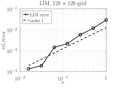
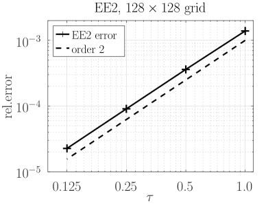
Figure 5: Error convergence plots for the LIM (left) and the EE2 (right) schemes run with constant time step size $\tau$ on the $128\times 128$ space grid. The plots are produced with the data from Table 1.

5.2 The LIM and EE2 schemes with a constant time step size

We first compare the two time integrators run with a constant time step size. It turns out that, for large constant time step sizes, small negative eigenvalues of $\widehat{A}_{n}$ may have a negative effect on the RT restarting procedure in the Krylov subspace methods. This is because the RT restarting procedure is guaranteed to work for matrices whose numerical range does not contain elements with negative real part (which is a typical assumption in analysis of Krylov subspace methods) [26, 27]. This problem can be solved by either reducing the time step size at an initial evolution phase or by using a large Krylov subspace dimension. For simplicity of the experiments, we choose to set the Krylov subspace dimension in the EE2 time integrator to a large value $m_{\max}=100$. We emphasize that this is done only if EE2 is used with a constant time step size. With the adaptive time stepping strategy we take either $m_{\max}=10$ or $m_{\max}=30$. As already discussed, taking the large value $m_{\max}=100$ makes comparing costs of both schemes in terms of the matrix-vector products with $\widehat{A}_{n}$ unfair. Hence, these values are given for indication only.

Table 1: Achieved accuracy and the number of spent matvecs (matrix-vector products) for the LIM and the EE2 schemes run with constant time step size $\tau$. The EE2 is not run with $\tau=0.0625$ because a high accuracy of convergence order 2 is observed for $\tau\geqslant 0.125$.

$\tau$	LIM		EE2
	# matvecs	error	# matvecs	error (tol)
$64\times 64$ grid
1.0	12960	9.60e-02	10217	3.24e-04 ($10^{-3}$)
0.5	18000	1.10e-03	24824	1.55e-04 ($10^{-5}$)
0.25	27856	2.52e-03	39138	3.88e-05 ($10^{-6}$)
0.125	40000	8.34e-04	63039	9.52e-06 ($10^{-7}$)
0.0625	48000	3.20e-04	—	—
$128\times 128$ grid
1.0	50770	2.90e-02	41266	1.60e-03 ($10^{-3}$)
0.5	69908	1.17e-02	92650	3.61e-04 ($10^{-5}$)
0.25	99824	5.70e-03	141148	9.08e-05 ($10^{-6}$)
0.125	136000	2.14e-03	210401	2.27e-05 ($10^{-7}$)
0.0625	207350	1.44e-03	—	—

To run with a constant $\tau$, the EE2 scheme needs a tolerance parameter $\texttt{tol}_{\varphi}$ for the Krylov subspace evaluation of the $\varphi$ matrix function. Therefore, we supply EE2 with a tolerance value tol, for which $\texttt{tol}_{\varphi}$ gets its value according to (31).

First, in Table 1 for both schemes we give values of the achieved accuracy, measured as in (32), and required number of matrix-vector products. Then, in Figure 5 error convergence plots for both schemes are presented. As we see, the EE2 scheme has indeed accuracy order 2 provided the linearized IVP (20) is solved at each time step sufficiently accurately (to achieve this, we decrease the tolerance value tol with the time step size $\tau$). The LIM scheme shows, as expected, at least an order 1 accuracy.

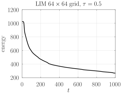
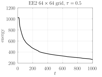
Figure 6: Discrete energy (33) versus time for the LIM (left) and EE2($\texttt{tol}=10^{-2}$) (right) schemes run with constant $\tau=0.5$

In Figure 6 for both schemes we show time evolution plots of discrete energy, computed on a $n_{x}\times n_{y}$ grid at each time step $n$ for $y^{n}=y$ as [17]

$$\mathcal{E}_{h}(y)=h_{x}h_{y}\sum_{i,j=1}^{n_{x},n_{y}}F(y_{i,j})+\frac{\epsilon^{2}}{2}\left(\sum_{i=0,j=1}^{n_{x},n_{y}}(y_{i+1,j}-y_{i,j})^{2}+\sum_{i=1,j=0}^{n_{x},n_{y}}(y_{i,j+1}-y_{i,j})^{2}\right),$$ (33)

with $h_{x,y}$ being the space grid sizes in the $x$ (respectively, $y$) direction. In addition, Figure 7 presents plots of mass deviation versus time in both schemes. To produce these figures, we intentionally take a large time step size $\tau=0.5$ and, for EE2, a relaxed tolerance value $\texttt{tol}=10^{-2}$: as we see, even in this case both schemes exhibit good conservation properties.

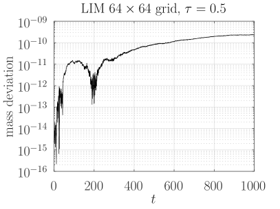
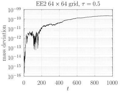
Figure 7: Mass deviation $|(m^{n}-m^{0})/m^{0}-1|$, with $m^{n}=\sum_{j}y_{j}^{n}$, versus time for the LIM (left) and EE2($\texttt{tol}=10^{-2}$) (right) schemes run with constant $\tau=0.5$

5.3 LIM and EE2 schemes with the Eyre splitting

We now present test results for the LIM and EE2 schemes combined with the Eyre splitting. Just as in the previous test, the EE2 scheme is provided with a tolerance parameter tol, for which the tolerance in the Krylov subspace method $\texttt{tol}_{\varphi}$ is determined by formula (31). The matrix $\widehat{A}_{n}$ is now similar to a symmetric positive semidefinite matrix and, hence, is guaranteed to have nonnegative eigenvalues (see Proposition 2), so that the RT restarting within the Krylov subspace evaluation of the matrix function $\varphi$ should now work reliably. Therefore, we set the maximal Krylov subspace dimension $m_{\max}$ to a realistic value $m_{\max}=30$ and denote the scheme with this $m_{\max}$ value as EE2(30). Choosing such a value of $m_{\max}$ allows to compare the costs in two schemes in terms of the needed matrix-vector multiplication number.

Error values achieved by both schemes, together with the number of required matrix-vector multiplications, are presented in Table 2. For the EE2(30) scheme, these data are obtained with a relaxed tolerance value $\texttt{tol}=10^{-2}$ which, taking into account the large error triggered by the Eyre splitting, appears to be sufficient. In the left plot of Figure 8, we plot the error values for both schemes versus the time step size $\tau$. The plot is produced with smaller tolerance values in the EE2 scheme, for which the error values have converged (i.e., decreasing tolerance further does not change the error value). The plot confirms a well known fact that the Eyre splitting has accuracy order 1. In the right plot of Figure 8, the error values reported in Table 2 are given versus the required matrix-vector multiplication number.

As we see, the EE2(30) scheme allows to achieve an accuracy comparable to that of the LIM scheme for much smaller number of matrix-vector multiplications. The price for this increased efficiency is storage and handling of $m_{\max}=30$ Krylov subspace vectors. As is clear from the results in the previous sections, the LIM and EE2 schemes have essentially different error behavior. Therefore, almost indistinguishable error convergence curves for the Eyre-stabilized LIM and EE2 schemes (see the left plot in Figure 8) are probably due to a large Eyre splitting error which dominates the errors in both schemes. Discrete energy, given by (33), and mass deviation plots for the EE2 scheme combined the Eyre splitting are presented in Figure 9.

Table 2: Achieved accuracy and the number of spent matvecs (matrix-vector products) for the LIM and the EE2($m_{\max}=30$) schemes combined with the Eyre splitting and run with constant time step size $\tau$.

$\tau$	LIM		EE2(30)
	# matvecs	error	# matvecs	error (tol)
$64\times 64$ grid
0.5	21878	9.93e-01	13776	4.84e-01 ($10^{-2}$)
0.25	28000	6.34e-01	17391	5.33e-01 ($10^{-2}$)
0.125	40000	5.05e-01	16965	6.67e-02 ($10^{-2}$)
0.0625	48000	7.47e-02	23910	2.41e-02 ($10^{-2}$)
0.03125	96000	3.85e-02	35818	1.13e-02 ($10^{-2}$)
$128\times 128$ grid
0.5	70000	8.02e-01	54973	7.98e-01 ($10^{-2}$)
0.25	100000	5.65e-01	66443	4.58e-02 ($10^{-2}$)
0.125	150444	3.06e-02	78237	2.92e-02 ($10^{-2}$)
0.0625	208000	1.84e-02	76857	2.16e-02 ($10^{-2}$)
0.03125	288000	1.03e-02	110008	1.15e-02 ($10^{-2}$)

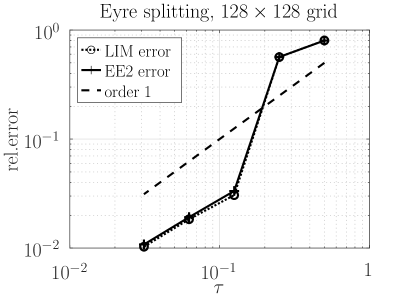
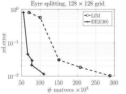
Figure 8: Left: error convergence rate for the LIM and EE2(30) combined with the Eyre splitting. Right: achieved error versus matrix-vector multiplication number for the LIM and EE2(30) combined with the Eyre splitting. The right plot is produced with the data from Table 2.

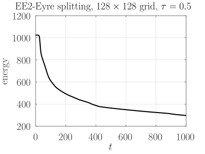
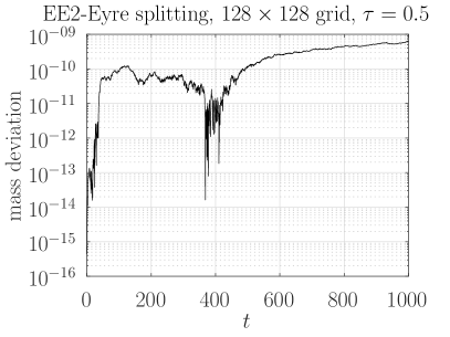
Figure 9: Discrete energy (33) (left) and mass deviation $|(m^{n}-m^{0})/m^{0}-1|$, with $m^{n}=\sum_{j}y_{j}^{n}$, (right) versus time for the EE2($m_{\max}=30$) scheme combined with the Eyre splitting and run with constant $\tau=0.5$ and $\texttt{tol}=10^{-2}$.

5.4 The LIM and EE2 schemes with adaptively chosen time step size

In this section both schemes are tested with time step size chosen adaptively as discussed in Sections 3.3.3 and 4.4.4. In this setting, a tolerance value tol is provided to both schemes which is then used to choose an appropriate time step size (cf. (18),(30)) and, in the EE2 scheme, also to determine the tolerance value $\texttt{tol}_{\varphi}$ for the Krylov subspace method in (31). In addition, both schemes are given an initial time step size $\tau_{0}$. In the EE2 scheme the value of $\tau_{0}$ can be instantly decreased by the Krylov subspace method while the time step is actually made, see Figure 3. That is why in the EE2 scheme we set $\tau_{0}$ to a large value $\tau_{0}=1$ in all the runs. The $\tau_{0}$ values used in the LIM scheme are reported. The maximal Krylov subspace dimension $m_{\max}$ in the EE2 scheme is set to either 10 or 30 and we denote the resulting scheme as EE2(10) and EE2(30), respectively.

Table 3: Achieved accuracy and the number of spent matvecs (matrix-vector products) for the LIM and the EE2 schemes run with adaptively chosen $\tau$ on the $128\times 128$ space grid. For the EE2 scheme initial time step size value is initially set to $\tau_{0}=1$ and instantly changed by the Krylov subspace method, see Figure 3. The maximal Krylov subspace dimension is $m_{\max}=10$ in EE2(10) and $m_{\max}=30$ in EE2(30).

method, tol ($\tau_{0}$)	# matvecs	error
LIM, $10^{-2}$ ($\tau_{0}=1.0$)	38940	2.73e-03
LIM, $10^{-3}$ ($\tau_{0}=0.5$)	120476	3.62e-04
LIM, $10^{-4}$ ($\tau_{0}=0.25$)	397133	1.22e-04
EE2(10), $10^{-2}$	42856	9.63e-03
EE2(10), $10^{-3}$	57100	3.31e-03
EE2(10), $10^{-4}$	110088	7.57e-05
EE2(30), $10^{-2}$	22800	4.62e-03
EE2(30), $10^{-3}$	44493	7.03e-04
EE2(30), $10^{-4}$	73867	1.28e-04

Table 4: Achieved accuracy and the number of spent matvecs (matrix-vector products) for the LIM and the EE2 schemes run with adaptively chosen $\tau$ on the $192\times 192$ space grid. For the EE2 scheme initial time step size value is initially set to $\tau_{0}=1$ and instantly changed by the Krylov subspace method, see Figure 3. The maximal Krylov subspace dimension is $m_{\max}=10$ in EE2(10) and $m_{\max}=30$ in EE2(30).

method, tol ($\tau_{0}$)	# matvecs	error
LIM, $10^{-2}$ ($\tau_{0}=1.0$)	85843	1.12e-03
LIM, $10^{-3}$ ($\tau_{0}=0.5$)	265411	1.82e-04
LIM, $10^{-4}$ ($\tau_{0}=0.25$)	893808	3.79e-05
EE2(10), $10^{-2}$	201460	1.07e-03
EE2(10), $10^{-3}$	208018	1.04e-03
EE2(10), $10^{-4}$	339418	4.33e-04
EE2(10), $10^{-5}$	546624	5.35e-06
EE2(30), $10^{-2}$	75053	2.99e-03
EE2(30), $10^{-3}$	126485	5.35e-04
EE2(30), $10^{-4}$	221243	1.21e-05

In Tables 3 and 4, for the space grids $128\times 128$ and $192\times 192$, respectively, we show achieved error values and corresponding required matrix-vector multiplication numbers. The data shown in the tables are also visualized in the error-versus-work plots in Figure 10. As we see, for moderate accuracy requirements the LIM scheme is slightly more efficient than the EE2(10) scheme. For stricter tolerance values the EE2(10) becomes more efficient than LIM. The EE2(30) outperforms both the LIM and EE2(10) schemes for the whole tolerance range.

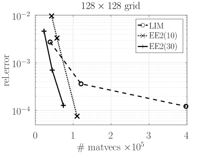
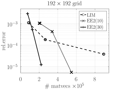
Figure 10: Achieved accuracy versus number of required matrix-vector products (matvecs) for the adaptive LIM, EE2(10) and EE2(30) schemes for $128\times 128$ (left) and $192\times 192$ (right) grids

In Figure 11 plots of the total energy versus time are presented for the adaptive LIM($\tau_{0}=1$) and EE2(10) schemes, where the discrete energy is computed according to (33). We deliberately produce these plots for both schemes run with a tolerance value $10^{-2}$: as we see, even with this moderate tolerance value the energy behavior in both schemes is adequate.

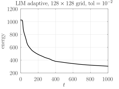
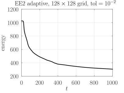
Figure 11: Discrete energy versus time for the adaptive LIM($\tau_{0}=1$) (left) and EE2(10) (right) schemes run with $\texttt{tol}=10^{-2}$

For the same runs of the adaptive LIM($\tau_{0}=1$) and EE2(10) schemes executed with the tolerance value $10^{-2}$, mass deviation plots are given in Figure 12. As we see, both scheme demonstrate quite acceptable mass conservation properties even with this relaxed tolerance value.

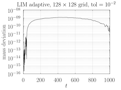
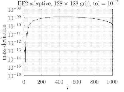
Figure 12: Mass deviation $|(m^{n}-m^{0})/m^{0}-1|$, with $m^{n}=\sum_{j}y_{j}^{n}$, versus time for the adaptive LIM($\tau_{0}=1$) (left) and EE2(10) (right) schemes run with $\texttt{tol}=10^{-2}$

Comparing the data in Tables 1 and 3 for the $128\times 128$ space grid, we see that the adaptive time step size selection yields an efficiency gain for the LIM scheme by approximately a factor 3.5 (for instance, 38940 instead of 136000 matrix-vector products to reach roughly the same accuracy). For the EE2 scheme the gain factor is up to approximately a factor 2 (e.g., 73867 instead of 141148 matrix-vector products to reach an accuracy $\approx 10^{-4}$).

6 Conclusions and an outlook to further research

In this paper an exponential time stepping scheme is proposed for numerical time integration of the Cahn–Hilliard equation. The scheme has a nonstiff accuracy order 2 and we call it exponential Euler order 2 scheme (EE2). It is explicit in the sense that it does not require linear system solution. We compare it to another explicit scheme, the local iteration modified (LIM) scheme [18, 19, 28], which is recently introduced for the Cahn–Hilliard equation in [30]. For both schemes we show how an adaptive time step size selection, similar to recently proposed in [31], can be implemented. We also describe how to combine both EE2 and LIM schemes with a variant of the Eyre convex splitting, for which we show similarity of the involved matrix to a symmetric positive semidefinite matrix.

Results of numerical experiments presented here allow to make the following conclusions.

1. When employed with a constant time step size and without the Eyre convex splitting, the LIM scheme works robustly, whereas the EE2 scheme has problems with growing Krylov subspace dimension due to instability (negative eigenvalues appearing in the Jacobian). With the maximal Krylov subspace dimension set to an unrealistically large value $m_{\max}=100$, the EE2 scheme delivers a significantly higher time integration accuracy than the LIM scheme for a comparable number of matrix-vector multiplications, see Table 1.

2. The Eyre convex splitting removes instability problems and allows to set the maximal Krylov subspace dimension in EE2 to a realistic value (we had $m_{\max}=30$ in the tests). However, combination with the Eye convex splitting significantly decreases accuracy in both the LIM and EE2 schemes. The EE2 scheme combined with the Eyre convex splitting appears to be more efficient than the LIM scheme combined with the Eyre splitting, see Figure 8.

3. The proposed adaptive time step size selection leads to an essential efficiency gain in both schemes: a gain factor is approximately 3.5 for the LIM scheme and around 2 for the EE2 scheme (compare Tables 1 and 3). The adaptive time step size selection also allows the EE2 scheme to deal with instability caused by small negative eigenvalues, while keeping the Krylov subspace dimension moderate ($m_{\max}=10$ and $m_{\max}=30$ in the tests) and without the Eyre splitting stabilization.

4. For low accuracy requirements ($\sim 10^{-3}$) the adaptive LIM scheme is slightly more efficient than the adaptive EE2 scheme with $m_{\max}=10$, see Figure 10. For higher accuracy requirements ($\leqslant 10^{-4}$) the adaptive EE2($m_{\max}=10$) scheme outperforms the adaptive LIM scheme. The adaptive EE2($m_{\max}=30$) scheme is essentially more efficient than the adaptive LIM scheme.

5. The LIM scheme does not require any parameter tuning, whereas the tolerance in the Krylov subspace method of the EE2 scheme has to be selected carefully, see formula (31). In overall, comparing the LIM and EE2 schemes, we conclude the EE2 scheme allows to increase efficiency significantly (up to a factor 4 less matrix-vector multiplications), at the cost of storing and handling $m_{\max}$ Krylov subspace vectors.

Future research can be aimed at improving the EE2 scheme, in particular, with respect to robustness of its Krylov subspace method for matrices having small negative ‘‘unstable’’ eigenvalues. A question whether higher order methods can be applicable and efficient for large-scale Cahn–Hilliard problems seems to be another promising research direction.

7 Funding

The authors of this work declare that their work was not financially supported.

8 CONFLICT OF INTEREST

The authors of this work declare that they have no conflicts of interest.

References

- [1] Y. Feng, Y. Feng, G. Iyer, and J.-L. Thiffeault, ‘‘Phase separation in the advective Cahn–Hilliard equation,’’ Journal of NonLinear Science, vol. 30, pp. 2821–2845, 2020. https://doi.org/10.1007/s00332-020-09637-6.
- [2] Q. Xia, J. Kim, and Y. Li, ‘‘Modeling and simulation of multi-component immiscible flows based on a modified Cahn–Hilliard equation,’’ European Journal of Mechanics-B/Fluids, vol. 95, pp. 194–204, 2022. https://doi.org/10.1016/j.euromechflu.2022.04.013.
- [3] L. Cherfils, H. Fakih, and A. Miranville, ‘‘A Cahn–Hilliard system with a fidelity term for color image inpainting,’’ Journal of Mathematical Imaging and Vision, vol. 54, pp. 117–131, 2016. https://doi.org/10.1007/s10851-015-0593-9.
- [4] S. M. Wise, J. S. Lowengrub, J. S. Kim, and W. C. Johnson, ‘‘Efficient phase-field simulation of quantum dot formation in a strained heteroepitaxial film,’’ Superlattices and Microstructures, vol. 36, no. 1-3, pp. 293–304, 2004. https://doi.org/10.1016/j.spmi.2004.08.029.
- [5] H. Garcke, T. Preusser, M. Rumpf, A. C. Telea, U. Weikard, and J. J. van Wijk, ‘‘A phase field model for continuous clustering on vector fields,’’ IEEE Transactions on Visualization and Computer Graphics, vol. 7, no. 3, pp. 230–241, 2001. https://doi.org/10.1109/2945.942691.
- [6] D. J. Eyre, ‘‘An unconditionally stable one-step scheme for gradient systems,’’ Unpublished article, vol. 6, 1998. https://citeseerx.ist.psu.edu/doc_view/pid/4f016a98fe25bfc06b9bcab3d85eeaa47d3ad3ca.
- [7] D. J. Eyre, ‘‘Unconditionally gradient stable time marching the Cahn–Hilliard equation,’’ MRS online proceedings library (OPL), vol. 529, p. 39, 1998. https://doi.org/10.1557/PROC-529-39.
- [8] B. P. Vollmayr-Lee and A. D. Rutenberg, ‘‘Fast and accurate coarsening simulation with an unconditionally stable time step,’’ Phys. Rev. E, vol. 68, no. 6, p. 066703, 2003. https://doi.org/10.1103/PhysRevE.68.066703.
- [9] S. M. Wise, C. Wang, and J. S. Lowengrub, ‘‘An energy-stable and convergent finite-difference scheme for the phase field crystal equation,’’ SIAM J. Numer. Anal., vol. 47, no. 3, pp. 2269–2288, 2009.
- [10] G. Tierra and F. Guillén-González, ‘‘Numerical methods for solving the Cahn-Hilliard equation and its applicability to related energy-based models,’’ Arch. Comput. Methods Eng., vol. 22, no. 2, pp. 269–289, 2015. https://doi.org/10.1007/s11831-014-9112-1.
- [11] G. N. Wells, E. Kuhl, and K. Garikipati, ‘‘A discontinuous Galerkin method for the Cahn–Hilliard equation,’’ J. Comput. Phys., vol. 218, no. 2, pp. 860–877, 2006. https://doi.org/10.1016/j.jcp.2006.03.010.
- [12] D. Kay and R. Welford, ‘‘A multigrid finite element solver for the Cahn–Hilliard equation,’’ J. Comput. Phys., vol. 212, no. 1, pp. 288–304, 2006. https://doi.org/10.1016/j.jcp.2005.07.004.
- [13] R. Guo and Y. Xu, ‘‘Efficient solvers of discontinuous Galerkin discretization for the Cahn–Hilliard equations,’’ J. Sci. Comput., vol. 58, pp. 380–408, 2014. https://doi.org/10.1007/s10915-013-9738-4.
- [14] J. Shen and X. Yang, ‘‘Numerical approximations of Allen–Cahn and Cahn–Hilliard equations,’’ Discrete Contin. Dyn. Syst, vol. 28, no. 4, pp. 1669–1691, 2010. http://dx.doi.org/10.3934/dcds.2010.28.1669.
- [15] M. Dehghan and V. Mohammadi, ‘‘The numerical solution of Cahn–Hilliard (CH) equation in one, two and three-dimensions via globally radial basis functions (GRBFs) and RBFs-differential quadrature (RBFs-DQ) methods,’’ Engineering Analysis with Boundary Elements, vol. 51, pp. 74–100, 2015. https://doi.org/10.1016/j.enganabound.2014.10.008.
- [16] A. M. Stuart and A. R. Humphries, ‘‘Model problems in numerical stability theory for initial value problems,’’ SIAM Rev., vol. 36, no. 2, pp. 226–257, 1994. https://doi.org/10.1137/1036054.
- [17] S. Lee, C. Lee, H. G. Lee, and J. Kim, ‘‘Comparison of different numerical schemes for the Cahn-Hilliard equation,’’ J. Korean Soc. Ind. Appl. Math., vol. 17, no. 3, pp. 197–207, 2013. https://doi.org/10.12941/jksiam.2013.17.197.
- [18] V. O. Lokutsievskii and O. V. Lokutsievskii, ‘‘On numerical solution of boundary value problems for equations of parabolic type,’’ Soviet Math. Dokl., vol. 34, no. 3, pp. 512–516, 1987. https://zbmath.org/?q=an:0637.65098.
- [19] A. S. Shvedov and V. T. Zhukov, ‘‘Explicit iterative difference schemes for parabolic equations,’’ Russian J. Numer. Anal. Math. Modelling, vol. 13, no. 2, pp. 133–148, 1998. https://doi.org/10.1515/rnam.1998.13.2.133.
- [20] B. P. Sommeijer, L. F. Shampine, and J. G. Verwer, ‘‘RKC: An explicit solver for parabolic PDEs,’’ J. Comput. Appl. Math., vol. 88, pp. 315–326, 1998. https://doi.org/10.1016/S0377-0427(97)00219-7.
- [21] V. I. Lebedev, ‘‘Explicit difference schemes for solving stiff systems of ODEs and PDEs with complex spectrum,’’ Russian J. Numer. Anal. Math. Modelling, vol. 13, no. 2, pp. 107–116, 1998. https://doi.org/10.1515/rnam.1998.13.2.107.
- [22] M. A. Botchev, G. L. G. Sleijpen, and H. A. van der Vorst, ‘‘Stability control for approximate implicit time stepping schemes with minimum residual iterations,’’ Appl. Numer. Math., vol. 31, no. 3, pp. 239–253, 1999. https://doi.org/10.1016/S0168-9274(98)00138-X.
- [23] J. G. Verwer, B. P. Sommeijer, and W. Hundsdorfer, ‘‘RKC time-stepping for advection–diffusion–reaction problems,’’ J. Comput. Phys., vol. 201, no. 1, pp. 61–79, 2004.
- [24] Y. Čžao Din, ‘‘On the stability of difference schemes for the solutions of parabolic differential equations,’’ Soviet Math. Dokl., vol. 117, pp. 578–581, 1958. https://zbmath.org/?q=an:0102.33501.
- [25] Y. Čžao Din, ‘‘Some difference schemes for the numerical solution of differential equations of parabolic type,’’ Mat. Sb., N. Ser., vol. 50, no. 92, pp. 391–422, 1960. https://www.mathnet.ru/rus/sm4800.
- [26] M. A. Botchev and L. A. Knizhnerman, ‘‘ART: Adaptive residual-time restarting for Krylov subspace matrix exponential evaluations,’’ J. Comput. Appl. Math., vol. 364, p. 112311, 2020. https://doi.org/10.1016/j.cam.2019.06.027.
- [27] M. A. Botchev, L. Knizhnerman, and E. E. Tyrtyshnikov, ‘‘Residual and restarting in Krylov subspace evaluation of the function,’’ SIAM J. Sci. Comput., vol. 43, no. 6, pp. A3733–A3759, 2021. https://doi.org/10.1137/20M1375383.
- [28] V. T. Zhukov, ‘‘Explicit methods of numerical integration for parabolic equations,’’ Math. Models Comput. Simul., vol. 3, no. 3, pp. 311–332, 2011. https://doi.org/10.1134/S2070048211030136.
- [29] M. A. Botchev and V. T. Zhukov, ‘‘On positivity of the local iteration modified time integration scheme,’’ Lobachevskii J. Math., 2025. To appear.
- [30] M. A. Botchev, I. A. Fahurdinov, and E. B. Savenkov, ‘‘Efficient and stable time integration of Cahn–Hilliard equations: Explicit, implicit, and explicit iterative schemes,’’ Comput. Math. and Math. Phys., vol. 64, pp. 1726–1746, 2024. https://doi.org/10.1134/S0965542524700945.
- [31] M. A. Botchev and V. T. Zhukov, ‘‘Adaptive iterative explicit time integration for nonlinear heat conduction problems,’’ Lobachevskii J. Math., vol. 45, no. 1, pp. 12–20, 2024. https://doi.org/10.1134/S1995080224010086.
- [32] R. A. Horn and C. R. Johnson, Matrix Analysis. Cambridge University Press, 1986.
- [33] E. Hairer, S. P. Nørsett, and G. Wanner, Solving Ordinary Differential Equations I. Nonstiff Problems. Springer Series in Computational Mathematics 8, Springer–Verlag, 1987.
- [34] O. B. Feodoritova, N. D. Novikova, and V. T. Zhukov, ‘‘On adaptive time step selection procedure for parabolic equations with the LIM scheme,’’ Lobachevskii J. Math., 2025. To appear.
- [35] V. L. Druskin and L. A. Knizhnerman, ‘‘Two polynomial methods of calculating functions of symmetric matrices,’’ U.S.S.R. Comput. Maths. Math. Phys., vol. 29, no. 6, pp. 112–121, 1989.
- [36] E. Gallopoulos and Y. Saad, ‘‘Efficient solution of parabolic equations by Krylov approximation methods,’’ SIAM J. Sci. Stat. Comput., vol. 13, no. 5, pp. 1236–1264, 1992.
- [37] M. Hochbruck and C. Lubich, ‘‘On Krylov subspace approximations to the matrix exponential operator,’’ SIAM J. Numer. Anal., vol. 34, pp. 1911–1925, Oct. 1997.
- [38] R. B. Sidje, ‘‘Expokit. A software package for computing matrix exponentials,’’ ACM Trans. Math. Softw., vol. 24, no. 1, pp. 130–156, 1998. www.maths.uq.edu.au/expokit/.
- [39] Y. Saad, Iterative Methods for Sparse Linear Systems. Book out of print, 2000. www-users.cs.umn.edu/˜saad/books.html.
- [40] H. A. van der Vorst, Iterative Krylov methods for large linear systems. Cambridge University Press, 2003.
- [41] N. J. Higham, Functions of Matrices: Theory and Computation. Philadelphia, PA, USA: Society for Industrial and Applied Mathematics, 2008.
- [42] E. Celledoni and I. Moret, ‘‘A Krylov projection method for systems of ODEs,’’ Appl. Numer. Math., vol. 24, no. 2-3, pp. 365–378, 1997. https://doi.org/10.1016/S0168-9274(97)00033-0.
- [43] V. L. Druskin, A. Greenbaum, and L. A. Knizhnerman, ‘‘Using nonorthogonal Lanczos vectors in the computation of matrix functions,’’ SIAM J. Sci. Comput., vol. 19, no. 1, pp. 38–54, 1998.
- [44] W. Hundsdorfer and J. G. Verwer, Numerical Solution of Time-Dependent Advection-Diffusion-Reaction Equations. Springer Verlag, 2003.
- [45] M. Hochbruck and A. Ostermann, ‘‘Exponential integrators,’’ Acta Numer., vol. 19, pp. 209–286, 2010.
- [46] E. Hairer and G. Wanner, Solving Ordinary Differential Equations II. Stiff and Differential–Algebraic Problems. Springer Series in Computational Mathematics 14, Springer–Verlag, 2 ed., 1996.