A Theory for Conditional Generative Modeling on Multiple Data Sources

Abstract

The success of large generative models has driven a paradigm shift, leveraging massive multi-source data to enhance model capabilities. However, the interaction among these sources remains theoretically underexplored. This paper takes the first step toward a rigorous analysis of multi-source training in conditional generative modeling, where each condition represents a distinct data source. Specifically, we establish a general distribution estimation error bound in average total variation distance for conditional maximum likelihood estimation based on the bracketing number. Our result shows that when source distributions share certain similarities and the model is expressive enough, multi-source training guarantees a sharper bound than single-source training. We further instantiate the general theory on conditional Gaussian estimation and deep generative models including autoregressive and flexible energy-based models, by characterizing their bracketing numbers. The results highlight that the number of sources and similarity among source distributions improve the advantage of multi-source training. Simulations and real-world experiments validate our theory. Code is available at: https://github.com/ML-GSAI/Multi-Source-GM.

1 Introduction

Large generative models have achieved remarkable success in generating realistic and complex outputs across natural language (Brown et al., 2020; Touvron et al., 2023) and computer vision (Rombach et al., 2022; OpenAI, 2024). A key factor behind their strong performance is the diverse and rich training data. For instance, large language models are trained on heterogeneous datasets comprising web content, books, and code (Brown et al., 2020; Hu et al., 2024b), while image generation models benefit from vast datasets spanning various categories and aesthetic qualities (Peebles & Xie, 2023; Chen et al., 2024; Esser et al., 2024). Empirical evidence suggests that, under certain conditions, training on multiple data sources can enhance performance across all sources (Pires et al., 2019; Chen et al., 2024; Allen-Zhu & Li, 2024a). Consequently, data mixture strategies have become an essential research topic (Nguyen et al., 2022; Chidambaram et al., 2022; Hu et al., 2024b).

However, the theoretical underpinnings of this multi-source training paradigm remain poorly understood. This raises a fundamental question: is it more effective to train separate models on individual data sources, or to train a single model using data from multiple sources? In this paper, we take the first step toward a rigorous analysis of multi-source training, focusing on its impact on conditional generative models, where each condition represents a distinct data source.

Our first contribution is establishing a general upper bound on distribution estimation error for conditional generative modeling via maximum likelihood estimation (MLE) in Section 3. Specifically, we measure the error using average total variation (TV) distance between the true and estimated conditional distributions across all sources, which scales as $\tilde{{\mathcal{O}}}(\sqrt{{\log{\mathcal{N}}_{{\mathcal{P}}_{X|Y}}}/{n}})$, where $n$ is the training set size and ${\mathcal{N}}_{{\mathcal{P}}_{X|Y}}$ is the bracketing number of the conditional distribution space ${\mathcal{P}}_{X|Y}$. Further, when source distributions exhibit parametric similarity, multi-source training effectively reduces the complexity of the distribution space, leading to a provably sharper bound than single-source training.

Technically, our analysis extends classical MLE estimation error bounds from empirical process theory (Wong & Shen, 1995; Geer, 2000; Ge et al., 2024) to the conditional setting by adapting the complexity of the distribution space and measuring the estimation error in terms of average TV distance. Further discussions are provided in Section 6.

As the second contribution, we instantiate our general theory in three specific cases: (1) parametric estimation of conditional Gaussian distributions, a simple example clearly illustrating how source distribution properties influence the benefits of multi-source training, (2) autoregressive models (ARMs), the foundation of large language models (Brown et al., 2020; Touvron et al., 2023), and (3) energy-based models (EBMs), a general class of generative models for continuous data (LeCun et al., 2006; Du & Mordatch, 2019; Song & Ermon, 2019). For each model, we derive explicit estimation error bounds for both multi-source and single-source training by measuring the bracketing number of corresponding conditional distribution space. Our theoretical results show that, across all cases, the ratio of multi-source to single-source estimation error bounds has a formulation $\sqrt{1-({K-1}/{K})\beta_{\mathrm{sim}}}$, where $K$ is the number of sources and $\beta_{\mathrm{sim}}\in[0,1]$ quantifies source distribution similarity, with model-specific definitions detailed in Section 4. This ratio decreases with both $K$ and $\beta_{\mathrm{sim}}$, indicating that the number of sources and their similarity improve the benefits of multi-source training.

A core technical contribution is establishing novel bracketing number bounds for ARMs and EBMs. This is challenging since on the one hand, the bracketing number provides a refined measure of function spaces, requiring carefully designed one-sided bounds over the entire domain. On the other hand, the conditional distribution space of deep generative models is inherently complex, involving both neural network architectures and specific probabilistic characteristics for different generative modeling methods. Please refer to Appendixes C and D for detailed proofs and discussions.

Finally, we validate our theoretical findings through simulations and real-world experiments in Section 5. In simulations, we perform conditional Gaussian estimation, where the MLE solutions can be analytically derived, enabling a rigorous assessment of the tightness of our bounds. The close match between the empirical and theoretical error orders supports the validity of our results. Beyond simulations, we train class-condition diffusion models (Karras et al., 2024) on ILSVRC2012 (Russakovsky et al., 2015) where its semantic hierarchy (Deng et al., 2010) provides a natural way to define inter-source distribution similarity. Empirical results confirm that multi-source training outperforms single-source training by achieving lower FID scores, consistent with our theoretical guarantee in Section 3, and this advantage depends on both the number of sources and their similarity, supporting our insights in Section 4.

2 Problem formulation

Elementary notations.

Scalars, vectors, and matrices are denoted by lowercase letters (e.g., $a$), lowercase boldface letters (e.g., ${\bm{a}}$), and uppercase boldface letters (e.g., ${\bm{A}}$). We use ${\bm{a}}[m]$ to denote the $m$-th entry of vector ${\bm{a}}$, and ${\bm{A}}[m,\mathrel{\mathop{\ordinarycolon}}]$, ${\bm{A}}[\mathrel{\mathop{\ordinarycolon}},n]$, and ${\bm{A}}[m,n]$ to denote the $m$-th row, the $n$-th column, and the entry at the $m$-th row and the $n$-th column of ${\bm{A}}$. $({\bm{a}},{\bm{b}})$ denotes the concatenation of ${\bm{a}}$ and ${\bm{b}}$ as a column vector. We denote $[n]\!\coloneqq\!\{1,\dots,n\}$ for any $n\in\mathbb{N}$ and $a\vee b$ as $\max\{a,b\}$. For any measurable scalar function $f({\bm{x}})$ on domain ${\mathscr{X}}$ and real number $1\leq\mathsf{p}\leq\infty$, its $L^{\mathsf{p}}({\mathscr{X}})$-norm is defined as $\lVert f({\bm{x}})\rVert_{L^{\mathsf{p}}({\mathscr{X}})}\!\coloneqq\!(\int_{{\mathscr{X}}}\lvert f({\bm{x}})\rvert^{\mathsf{p}}\,d{\bm{x}})^{\frac{1}{\mathsf{p}}}.$ When $\mathsf{p}\!=\!\infty$, $\lVert f({\bm{x}})\rVert_{L^{\infty}({\mathscr{X}})}\!=\!\sup_{{\bm{x}}\in{\mathscr{X}}}\lvert f({\bm{x}})\rvert$. $\mathbb{I}(\cdot)$ denotes the indicator function. Notation $a_{n}\!=\!\tilde{{\mathcal{O}}}(b_{n})$ indicates $a_{n}$ is asymptotically bounded above by $b_{n}$ up to logarithmic factors.

2.1 Data from multiple sources

Let $X$ denote the random variable for data (e.g., a natural image) in a data space ${\mathscr{X}}$, and $Y$ denote the random variable for the source label in a label space ${\mathscr{Y}}$. Suppose there are $K$ data sources (e.g., $K$ categories of images), each corresponding to an unknown conditional distribution $p^{*}_{X|k}$ for $k\in[K]$. We assume that $p^{*}_{X|k}$ is parameterized by a source-specific feature $\phi_{k}^{*}$ in a parameter space $\Phi$ and a shared feature $\psi^{*}$ in a parameter space $\Psi$, such that $p^{*}_{X|k}(x|k)=p_{\phi_{k}^{*},\psi^{*}}(x|k)$. The conditional distribution of $X$ given $Y=y$ is consequently expressed as

$$p^{*}_{X|Y}({\bm{x}}|y)=\prod_{k=1}^{K}\!\left(p_{\phi_{k}^{*},\psi^{*}}({\bm{x}}|k)\right)^{\mathbb{I}(y=k)}.$$

This compact representation provides convenience for subsequent discussions.

We further assume the distribution of $Y$ is known since the proportion of data from different sources is often manually designed in practice (Deng et al., 2009; Krizhevsky et al., 2009; Brown et al., 2020; Chen et al., 2024). The joint distribution of $X$ and $Y$ is then given by $p^{*}_{X,Y}({\bm{x}},y)=p^{*}_{X|Y}({\bm{x}}|y)p^{*}_{Y}(y)$.

2.2 Conditional generative modeling

Consider a dataset $S=\{({\bm{x}}_{i},y_{i})\}_{i=1}^{n}$ consisting of $n$ independent and identically distributed (i.i.d.) data-label pairs sampled from the joint distribution $p^{*}_{X,Y}$. In the learning phase, a conditional generative model uses maximum likelihood estimation (MLE) to estimate $p^{*}_{X|Y}$ based on the dataset $S$, where the conditional likelihood is defined as

$${\mathcal{L}}_{S}(p_{X|Y})\coloneqq\prod_{i=1}^{n}p_{X|Y}({\bm{x}}_{i}|y_{i}).$$ (1)

Multi-source training.

Under multi-source training, the conditional distribution space is given by ${\mathcal{P}}_{X|Y}^{\mathrm{multi}}\coloneqq$

$$\textstyle{\left\{p_{X|Y}^{\mathrm{multi}}({\bm{x}}|y)\!=\!\prod_{k=1}^{K}\left(p_{\phi_{k},\psi}({\bm{x}}|k)\right)^{\mathbb{I}(y=k)}\!\mathrel{\mathop{\ordinarycolon}}\!\phi_{k}\!\in\!\Phi,\!\psi\!\in\!\Psi\right\},}$$

and the corresponding estimator of $p^{*}_{X|Y}$ is

$$\hat{p}_{X|Y}^{\mathrm{multi}}=\operatorname*{arg\,max}_{p_{X|Y}^{\mathrm{multi}}\in{\mathcal{P}}_{X|Y}^{\mathrm{multi}}}{\mathcal{L}}_{S}(p_{X|Y}^{\mathrm{multi}}).$$ (2)

Here, we adopt the realizable assumption that true parameters satisfy $\phi_{k}^{*}\in\Phi$ and $\psi^{*}\in\Psi$ following (Ge et al., 2024), which allows the estimation error analysis to focus on the generalization property of the distribution space.

Single-source training.

Under single-source training, we train $K$ conditional generative models for each source using data exclusively from the corresponding source. For any particular source $k$, denoting $S_{k}\coloneqq\{({\bm{x}}_{i},y_{i})\in S|y_{i}=k\}=\{{\bm{x}}_{j}^{k},k\}_{j=1}^{n_{k}}$, the corresponding generative model estimate $p^{*}_{X|k}$ by maximizing the conditional likelihood on $S_{k}$ as

$$\hat{p}_{X|k}^{\mathrm{single}}=\operatorname*{arg\,max}_{p_{X|k}^{\mathrm{single}}\in{\mathcal{P}}_{X|k}^{\mathrm{single}}}{\mathcal{L}}_{S_{k}}(p_{X|k}^{\mathrm{single}}),$$

where ${\mathcal{L}}_{S_{k}}(p_{X|k})\coloneqq\prod_{j=1}^{n_{k}}p_{X|k}({\bm{x}}_{j}^{k}|k)$ and ${\mathcal{P}}_{X|k}^{\mathrm{single}}\coloneqq\left\{p_{\phi_{k},\psi_{k}}({\bm{x}}|k)\mathrel{\mathop{\ordinarycolon}}\phi_{k}\in\Phi,\psi_{k}\in\Psi\right\}$.

Separately maximizing these $K$ objectives is equivalent to finding the maximizer of $L_{S}$ in conditional distribution space ${\mathcal{P}}_{X|Y}^{\mathrm{single}}\coloneqq$

$$\textstyle{\left\{p_{X|Y}^{\mathrm{single}}({\bm{x}}|y)\!=\!\!\prod_{k=1}^{K}\left(p_{\phi_{k},\psi_{k}}({\bm{x}}|k)\right)^{\mathbb{I}(y=k)}\!\mathrel{\mathop{\ordinarycolon}}\!\phi_{k}\!\in\!\Phi,\psi_{k}\!\!\in\!\Psi\!\right\}.}$$

Therefore, the estimator of $p^{*}_{X|Y}$ under single-source training is

$$\hat{p}_{X|Y}^{\mathrm{single}}=\operatorname*{arg\,max}_{p_{X|Y}^{\mathrm{single}}\in{\mathcal{P}}_{X|Y}^{\mathrm{single}}}{\mathcal{L}}_{S}(p_{X|Y}^{\mathrm{single}}).$$ (3)

The introduced multi-source setting abstracts practical scenarios where different sources share certain underlying data structures (via $\psi$) while retaining unique characteristics (via $\phi_{k}$). At the same time, the single-source setting provides a controlled comparison to rigorously assess whether incorporating other sources improves the model’s learning.

Evaluation for conditional distribution estimation.

We measure the accuracy of conditional distribution estimation by average TV distance between the estimated and true conditional distributions, referred to as average TV error:

$${\mathcal{R}}_{\overline{\mathrm{TV}}}(\hat{p}_{X|Y})\coloneqq\mathbb{E}_{Y}\left[\mathrm{TV}(\hat{p}_{X|Y},p^{*}_{X|Y})\right],$$ (4)

where $\mathrm{TV}(\hat{p}_{X|Y},p^{*}_{X|Y})\!=\!\frac{1}{2}\!\int_{{\mathscr{X}}}\!|\hat{p}_{X|Y}({\bm{x}}|y)\!-\!p^{*}_{X|Y}({\bm{x}}|y)|d{\bm{x}}$ is the total variation distance between $\hat{p}_{X|Y}$ and $p^{*}_{X|Y}$.

In the following sections, we investigate the effectiveness of multi-source training by measuring and comparing ${\mathcal{R}}_{\overline{\mathrm{TV}}}(\hat{p}^{\mathrm{multi}}_{X|Y})$ and ${\mathcal{R}}_{\overline{\mathrm{TV}}}(\hat{p}^{\mathrm{single}}_{X|Y})$.

3 Provable advantage of multi-source training

In this section, we establish a general upper bound on the average TV error for conditional MLE and provide a statistical guarantee for the benefits of multi-source training. Our analysis extends the classical MLE guarantees (Geer, 2000; Ge et al., 2024), which leverage the bracketing number and the uniform law of large numbers.

3.1 Complexity of the conditional distribution space

We begin by introducing an extended notion of the bracketing number as follows.

Definition 3.1 ($\epsilon$-upper bracketing number for conditional distribution space).

Let $\epsilon$ be a real number that $\epsilon>0$ and $\mathsf{p}$ be an integer that $1\leq\mathsf{p}\leq\infty$. An $\epsilon$-upper bracket of a conditional distribution space ${\mathcal{P}}_{X|Y}$ with respect to $L^{\mathsf{p}}({\mathscr{X}})$ is a finite function set ${\mathcal{B}}$ such that for any $p_{X|Y}\in{\mathcal{P}}_{X|Y}$, there exists some $p^{\prime}\in{\mathcal{B}}$ such that given any $y\in{\mathscr{Y}}$, it holds

$$\forall{\bm{x}}\in{\mathscr{X}}\mathrel{\mathop{\ordinarycolon}}p^{\prime}({\bm{x}},y)\geq p_{X|Y}({\bm{x}}|y),\text{ and }$$

$$\lVert p^{\prime}(\cdot,y)-p_{X|Y}(\cdot|y)\rVert_{L^{\mathsf{p}}({\mathscr{X}})}\leq\epsilon.$$

The $\epsilon$-upper bracketing number ${\mathcal{N}}_{[]}\left(\epsilon;{\mathcal{P}}_{X|Y},L^{\mathsf{p}}({\mathscr{X}})\right)$ is the cardinality of the smallest $\epsilon$-upper bracket.

This notion quantifies the minimal set of functions needed to upper bound every conditional distribution within a small margin, reducing error analysis from an infinite to a finite function class. Unlike traditional bracketing numbers for unconditional distributions $p_{X}$ using two-sided brackets (Wellner, 2002), this extension employs one-sided upper brackets (Ge et al., 2024) and requires uniform coverage across $y$ for all conditional distributions tailored for our setting.

3.2 Guarantee for conditional MLE

We now present a general error bound which applies to both training strategies.

Theorem 3.2 (Average TV error bound for conditional MLE, proof in Section A.1).

Given a dataset $S$ of size $n$ that i.i.d. sampled from $p^{*}_{X,Y}$, let $\hat{p}_{X|Y}$ be the maximizer of $L_{S}(p_{X|Y})$ defined in Equation 1 in conditional distribution space ${\mathcal{P}}_{X|Y}$. Suppose the real conditional distribution $p^{*}_{X|Y}$ is contained in ${\mathcal{P}}_{X|Y}$. Then, for any $0<\delta\leq 1/2$, it holds with probability at least $1-\delta$ that

$${\mathcal{R}}_{\overline{\mathrm{TV}}}(\hat{p}_{X|Y}\!)\!\leq\!3\sqrt{\!\frac{1}{n}\left(\log{\mathcal{N}}_{[]}\left(\!\frac{1}{n};{\mathcal{P}}_{X|Y},L^{1}({\mathscr{X}})\!\!\right)\!\!+\!\log\frac{1}{\delta}\!\right)}.$$

As formulated in Equation 2 and Equation 3, multi-source and single-source training apply conditional MLE on $S$ within different conditional distribution spaces. The following proposition shows that multi-source training reduces the bracketing number of its distribution space through source similarity.

Proposition 3.3 (Multi-source training reducing complexity, proof in Section A.2.).

Let ${\mathcal{P}}_{X|Y}^{\mathrm{multi}}$ and ${\mathcal{P}}_{X|Y}^{\mathrm{single}}$ be as defined in Section 2. Then, for any $\epsilon>0$ and $1\leq\mathsf{p}\leq\infty$, we have

$${\mathcal{N}}_{[]}\left(\epsilon;{\mathcal{P}}_{X|Y}^{\mathrm{multi}},L^{\mathsf{p}}({\mathscr{X}})\right)\leq{\mathcal{N}}_{[]}\left(\epsilon;{\mathcal{P}}_{X|Y}^{\mathrm{single}},L^{\mathsf{p}}({\mathscr{X}})\right).$$

Combining Theorem 3.2 and Proposition 3.3, we conclude that when source distributions have parametric similarity and the model satisfies the realizable assumption, multi-source training can enjoy a sharper estimation guarantee than single-source training. Simulations and real-world experiments in Section 5 support our result.

4 Instantiations

We now apply our general analysis to conditional Gaussian estimation and two deep generative models to obtain concrete error bounds.

4.1 Parametric estimation on Gaussian distributions

As employed in extensive work (Montanari & Saeed, 2022; Wang & Thrampoulidis, 2022; He et al., 2022; Zheng et al., 2023; Dandi et al., 2024), Gaussian models provide a simple yet insightful case for illustrating the benefits of multi-source training and enable analytically tractable simulations under our theoretical assumptions.

Parametric distribution family.

Suppose each of the $K$ conditional distributions is a $d$-dimensional standard Gaussian distribution, i.e.,

$$\forall k\in[K],\quad X|k\sim{\mathcal{N}}(\bm{\mu}_{k}^{*},{\bm{I}}_{d})=(2\pi)^{-\frac{d}{2}}e^{-\frac{1}{2}\lVert{\bm{x}}-\bm{\mu}_{k}^{*}\rVert_{2}^{2}},$$

with a mean vector $\bm{\mu}_{k}^{*}$ and an identity covariance matrix ${\bm{I}}_{d}\in\mathbb{R}^{d\times d}$. We assume each mean vector has two parts: the first $d_{1}$ entries $\bm{\mu}_{k}^{*}[1\!\mathrel{\mathop{\ordinarycolon}}\!d_{1}]$ represent the source-specific feature which is potentially different for each source, and the remaining entries $\bm{\mu}_{k}^{*}[d_{1}\!+\!1\!\mathrel{\mathop{\ordinarycolon}}\!d]$ represent the shared feature which is identical across all sources. Corresponding to the general formulation in Section 2, we denote

$$\phi_{k}\!\coloneqq\!\bm{\mu}_{k}^{*}[1\mathrel{\mathop{\ordinarycolon}}d_{1}],\psi\!\coloneqq\!\bm{\mu}_{1}^{*}[d_{1}\!+\!1\!\mathrel{\mathop{\ordinarycolon}}\!d]\!=\!\cdots\!=\!\bm{\mu}_{K}^{*}[d_{1}\!+\!1\!\mathrel{\mathop{\ordinarycolon}}\!d],$$

and the conditional distribution is parameterized as

$$p_{\phi_{k},\psi}({\bm{x}}|k)=(2\pi)^{-\frac{d}{2}}e^{-\frac{1}{2}\lVert{\bm{x}}-(\phi_{k},\psi)\rVert_{2}^{2}}.$$ (5)

Statistical guarantee of the average TV error.

In this formulation, the conditional MLE in ${\mathcal{P}}_{X|Y}^{\mathrm{multi}}$ under multi-source training leads to the following result.

Theorem 4.1 (Average TV error bound for conditional Gaussian estimation under multi-source training, proof in Section B.2).

Let $\hat{p}_{X|Y}^{\mathrm{multi}}$ be the likelihood maximizer defined in Equation 2 given ${\mathcal{P}}_{X|Y}^{\mathrm{multi}}$ with conditional distributions as in Equation 5. Suppose $\Phi=[-B,B]^{d_{1}}$, $\Psi=[-B,B]^{d-d_{1}}$ with constant $B>0$, and $\phi_{k}^{*}\in\Phi$, $\psi^{*}\in\Psi$. Then, for any $0<\delta\leq 1/2$, it holds with probability at least $1-\delta$ that

$${\mathcal{R}}_{\overline{\mathrm{TV}}}(\hat{p}_{X|Y}^{\mathrm{multi}})=\tilde{{\mathcal{O}}}\left(\sqrt{\frac{(K-1)d_{1}+d}{n}}\right).$$

In contrast, single-source training results in an error of ${\mathcal{R}}_{\overline{\mathrm{TV}}}(\hat{p}_{X|Y}^{\mathrm{single}})=\tilde{{\mathcal{O}}}\left(\sqrt{{Kd}/{n}}\right)$, with a formal result provided in Theorem B.2. The advantage of multi-source learning can be quantified by the ratio of error bounds: ${\sqrt{\frac{(K-1)d_{1}+d}{Kd}}}=\sqrt{1-\frac{K-1}{K}\frac{d-d_{1}}{d}}.$ Denoting $\beta_{\mathrm{sim}}\coloneqq\frac{d-d_{1}}{d}$, this general form of ratio $\sqrt{1-\frac{K-1}{K}\beta_{\mathrm{sim}}}$ applies across Section 4.2 and Section 4.3, decreasing with both the number of sources $K$ and source similarity $\beta_{\mathrm{sim}}$.

Specifically, as $K$ increases from $1$ to $\infty$, the ratio decreases from $1$ to $\sqrt{1-\beta_{\mathrm{sim}}}$, and as $\beta_{\mathrm{sim}}$ increases from $0$ (completely dissimilar distributions) to $1$ (completely identical distributions), it decreases from $1$ to $\sqrt{1/K}$, reflecting a transition from no asymptotic gain to a constant improvement. This highlights that the number of sources and distribution similarity enhance the benefits of multi-source training. Empirical results in Section 5.2 confirm this trend.

4.2 Conditional ARMs on discrete distributions

For deep generative models, our formulations are based on multilayer perceptrons (MLPs), a fundamental network component, with potential extensions to Transformers and convolution networks with existing literature (Lin & Zhang, 2019; Ledent et al., 2021; Shen et al., 2021; Hu et al., 2024a; Trauger & Tewari, 2024; Jiao et al., 2024). We formally define MLPs mainly following notations in  Oko et al. (2023)

Definition 4.2 (Class of MLPs).

A class of MLPs ${\mathcal{F}}(L,W,S,B)$ with depth $L$, width $W$, sparsity $S$, norm $B$, and element-wise ReLU activation that $\mathrm{ReLU}(x)=0\vee x$ is defined as ${\mathcal{F}}(L,W,S,B)\!\coloneqq\!\{{\bm{f}}({\bm{x}})\!=\!({\bm{A}}^{(L)}\mathrm{ReLU}(\cdot)\!+\!{\bm{b}}^{(L)})\circ\cdots\circ({\bm{A}}^{(1)}{\bm{x}}\!+\!{\bm{b}}^{(1)})\!\mathrel{\mathop{\ordinarycolon}}\!\{({\bm{A}}^{(l)},{\bm{b}}^{(l)})\}_{l=1}^{L}\!\in\!{\mathcal{W}}(L,W,S,B)\}$, where parameter space ${\mathcal{W}}(L,W,S,B)$ is defined by ${\mathcal{W}}(L,W,S,B)\coloneqq\{\{({\bm{A}}^{(l)},{\bm{b}}^{(l)})\}_{l=1}^{L}\mathrel{\mathop{\ordinarycolon}}{\bm{A}}^{(l)}\in\mathbb{R}^{W_{l}\times W_{l-1}},{\bm{b}}^{(l)}\in\mathbb{R}^{W_{l}},\max_{l}W_{l}\leq W,\sum_{l=1}^{L}(\lVert{\bm{A}}^{(l)}\rVert_{0}+\lVert{\bm{b}}^{(l)}\rVert_{0})\leq S,\max_{l}\lVert{\bm{A}}^{(l)}\rVert_{\infty}\vee\lVert{\bm{b}}^{(l)}\rVert_{\infty}\leq B\}$.

We now present the formulation for ARMs, which can be viewed as an extension of Uria et al. (2016).

Probabilistic modeling with autoregression.

Consider a common data scenario for the natural language where $X$ represents a $D$-length text in $[M]^{D}$. Each dimension of $X$ is an integer token following an $M$-categorical distribution with $M$ being the vocabulary size. Adopting the autoregressive approach of probabilistic modeling, conditional distribution $p_{X|Y}({\bm{x}}|y)$ is factorized using the chain rule as:

$$p({\bm{x}}|y) =p\left(x_{1}|y\right)\cdots p\left(x_{D}|{\bm{x}}_{<D},y\right)$$

$$=p\left(x_{1};\bm{\rho}(y)\right)\cdots p\left(x_{D};\bm{\rho}({\bm{x}}_{<D},y)\right).$$

We omit the subscripts for notation simplicity. Here, for any $d\in[D]$, $\bm{\rho}(x_{<d},y)$ is the distribution parameter for $X_{d}$ given $X_{<d},Y\!=\!{\bm{x}}_{<d},y$ that

$$p\left(x_{d}=m|{\bm{x}}_{<d},y\right)=\bm{\rho}({\bm{x}}_{<d},y)[m],$$

satisfying $\bm{\rho}({\bm{x}}_{<d},y)\in\mathbb{R}_{+}^{M}$ and $\sum_{m=1}^{M}\bm{\rho}({\bm{x}}_{<d},y)[m]=1$.

Distribution estimation via neural network.

Aligning with common practices, we suppose the distribution parameter vector is estimated with $\bm{\rho}_{{\theta}}(x_{<d},y)$ using a shared neural network parameterized by ${\theta}$ across all dimensions. The network comprises an embedding layer, an encoding layer, an MLP block, and a softmax output layer.

Specifically, we first look up ${\bm{x}}$ and $y$ in two embedding matrices ${\bm{V}}_{X}\in[0,1]^{M\times d_{\mathrm{e}}}$ and ${\bm{V}}_{Y}\in[0,1]^{K\times d_{\mathrm{e}}}$, then stack the embeddings to get

$${\bm{E}}_{{\bm{V}}_{Y},{\bm{V}}_{X}}({\bm{x}},y)=\begin{bmatrix}{\bm{V}}_{Y}[y,\mathrel{\mathop{\ordinarycolon}}]\\ {\bm{V}}_{X}[x_{1},\mathrel{\mathop{\ordinarycolon}}]\\ \vdots\\ {\bm{V}}_{X}[x_{D-1},\mathrel{\mathop{\ordinarycolon}}]\end{bmatrix}\in[0,1]^{D\times d_{\mathrm{e}}},$$

where the last dimension of $x$ is excluded since it is not used when estimating the distribution.

Subsequently, we encode each embedding by a linear transformation with parameters ${\bm{A}}_{0}\in\mathbb{R}^{D\times d_{\mathrm{e}}}$, ${\bm{b}}_{0}\in\mathbb{R}^{D}$ and normalize the output with an element-wise sigmoid function $\sigma(x)=\frac{1}{1+e^{-x}}$ as

$${\bm{v}}_{{\bm{A}}_{0},{\bm{b}}_{0}}({\bm{E}}_{{\bm{V}}_{Y},{\bm{V}}_{X}}({\bm{x}},y))$$

$$=\begin{bmatrix}\sigma\left({\bm{A}}_{0}[1,\mathrel{\mathop{\ordinarycolon}}]{\bm{V}}_{Y}[y,\mathrel{\mathop{\ordinarycolon}}]^{\top}\!+\!{\bm{b}}_{0}[1]\right)\\ \vdots\\ \sigma\left({\bm{A}}_{0}[D,\mathrel{\mathop{\ordinarycolon}}]{\bm{V}}_{X}[x_{D-1},\mathrel{\mathop{\ordinarycolon}}]^{\top}\!+\!{\bm{b}}_{0}[D]\right)\end{bmatrix}\in[0,1]^{D}.$$

To ensure no components related to ${\bm{x}}_{\geq d}$ is seen when estimating the conditional probability for $x_{d}$, we mask ${\bm{v}}_{{\bm{A}}_{0},{\bm{b}}_{0}}$ using a $(D-d)$-dimensional zero vector $\bm{0}_{D-d}$ as

$${\bm{v}}_{{\bm{A}}_{0},{\bm{b}}_{0}}^{\backslash\bm{0}_{D-d}}\coloneqq\begin{bmatrix}{\bm{v}}_{{\bm{A}}_{0},{\bm{b}}_{0}}[1\mathrel{\mathop{\ordinarycolon}}d]^{\top}\ \bm{0}_{D-d}^{\top}\end{bmatrix}^{\top}.$$

Then we calculate the distribution parameter vector by an MLP ${\bm{f}}_{{\omega}}\!\in\!{\mathcal{F}}(L,W,S,B)$ with $W_{0}\!=\!D$ and $W_{L}\!=\!M$, followed by a softmax layer as

$$\bm{\rho}_{{\theta}}({\bm{x}}_{<d},\!y)\!=\!\mathrm{softmax}\left(\!{\bm{f}}_{{\omega}}\left(\!{\bm{v}}_{{\bm{A}}_{0},{\bm{b}}_{0}}^{\backslash\bm{0}_{D-d}}\!\left({\bm{E}}_{{\bm{V}}_{Y},{\bm{V}}_{X}}\!({\bm{x}},y)\!\right)\!\right)\!\!\right),$$

This leads to conditional distribution as

$$p_{{\theta}}\left({\bm{x}}|y\right)=p\left(x_{1};\bm{\rho}_{{\theta}}(y)\right)\cdots p\left(x_{D};\bm{\rho}_{{\theta}}({\bm{x}}_{<D},y)\right).$$ (6)

When training such an ARM, each row of ${\bm{V}}_{Y}$ is only optimized on data with the corresponding condition, while parameters in ${\bm{V}}_{X},{\bm{A}}_{0},{\bm{b}}_{0}$, and ${\omega}$ are optimized on data with all conditions. That means ${\bm{V}}_{Y}[k,\mathrel{\mathop{\ordinarycolon}}]$ serves as the source-specific parameter, while other parameters are shared across all sources. Corresponding to the general formulation in Section 2, we denote

$$\phi_{k}\coloneqq{\bm{V}}_{Y}[k,\mathrel{\mathop{\ordinarycolon}}],\ \text{and }\psi\coloneqq\{{\bm{V}}_{X},{\bm{A}}_{0},{\bm{b}}_{0},{\omega}\}.$$

Statistical guarantee of the average TV error.

In this formulation, the conditional MLE in ${\mathcal{P}}_{X|Y}^{\mathrm{multi}}$ under multi-source training leads to the following result.

Theorem 4.3 (Average TV error bound for ARMs under multi-source training, proof in Section C.4).

Let $\hat{p}_{X|Y}^{\mathrm{multi}}$ be the likelihood maximizer defined in Equation 2 given ${\mathcal{P}}_{X|Y}^{\mathrm{multi}}$ with conditional distributions as in Equation 6. Suppose $\Phi\!=\![0,1]^{d_{\mathrm{e}}}$, $\Psi\!=\![0,1]^{M\times d_{\mathrm{e}}}\!\times\![-B,B]^{D\times d_{\mathrm{e}}}\!\times\![-B,B]^{D}\!\times\!{\mathcal{W}}(L,W,S,B)$ with constants $L,W,S,B>0$, and $\phi_{k}^{*}\in\Phi$, $\psi^{*}\in\Psi$. Then, for any $0<\delta\leq 1/2$, it holds with probability at least $1-\delta$ that

$${\mathcal{R}}_{\overline{\mathrm{TV}}}(\hat{p}_{X|Y}^{\mathrm{multi}})=\tilde{{\mathcal{O}}}\left(\sqrt{\frac{L\left(S+D+(D+M+K)d_{\mathrm{e}}\right)}{n}}\right).$$

In contrast, single-source training results in an error of ${\mathcal{R}}_{\overline{\mathrm{TV}}}(\hat{p}_{X|Y}^{\mathrm{single}})=\tilde{{\mathcal{O}}}\left(\sqrt{{KL(S\!+\!D\!+\!(D\!+\!M\!+\!1)d_{\mathrm{e}})}/{n}}\right)$ with a formal result provided in Theorem C.8. The advantage of multi-source learning is quantified by the ratio of error bounds: $\sqrt{\frac{L(S+D+(D+M+K)d_{\mathrm{e}})}{KL(S+D+(D+M+1)d_{\mathrm{e}})}}=\sqrt{1\!-\!\frac{K-1}{K}\beta_{\mathrm{sim}}}$, where the term $\beta_{\mathrm{sim}}\coloneqq\frac{S+D+(D+M)d_{\mathrm{e}}}{S+D+(D+M+K)d_{\mathrm{e}}+d_{\mathrm{e}}}\in[0,1]$ quantifies source distribution similarity based on the proportion of shared parameters. This ratio follows the same pattern discussed in Section 4.1 where the number of sources $K$ and the distribution similarity $\beta_{\mathrm{sim}}$ are two key factors improving the advantage of multi-source training.

4.3 Conditional EBMs on continuous distributions

In this section, we study distribution estimation for conditional EBMs, a flexible probabilistic modeling approach on continuous data. Our formulation follows Du & Mordatch (2019) with simplified neural network architecture.

Probabilistic modeling with energy function.

Consider a common scenario with natural image $X$ flattened and normalized in $[0,1]^{D}$. The conditional distribution $p_{X|Y}({\bm{x}}|y)$ is factorized with an energy function $u({\bm{x}}|y)$ as:

$$p({\bm{x}}|y)=\frac{e^{-u({\bm{x}}|y)}}{\int_{{\mathscr{X}}}e^{-u({\bm{s}}|y)}d{\bm{s}}}.$$

Distribution estimation via neural network.

We suppose the energy function is estimated with $u_{{\theta}}({\bm{x}}|y)$ using a neural network parameterized by ${\theta}$, which comprises a condition embedding layer and an energy-estimating MLP.

Specifically, we first look up $y$ in a condition embedding matrix ${\bm{V}}\in[0,1]^{K\times d_{\mathrm{e}}}$ and concat the embedding with ${\bm{x}}$

$${\bm{e}}_{{\bm{V}}}({\bm{x}},y)=\begin{bmatrix}{\bm{x}}\\ {\bm{V}}[y,\mathrel{\mathop{\ordinarycolon}}]\end{bmatrix}\in[0,1]^{D+d_{\mathrm{e}}}.$$

Then we use an MLP $f_{{\omega}}\in{\mathcal{F}}(L,W,S,B)$ with $W_{0}=D+d_{\mathrm{e}}$ and $W_{L}=1$ to estimate the energy as

$$u_{{\theta}}({\bm{x}}|y)=f_{{\omega}}\left({\bm{e}}_{{\bm{V}}}({\bm{x}},y)\right),$$

where ${\theta}\coloneqq\{{\bm{V}},{\omega}\}$. This leads to a conditional distribution as

$$p_{{\theta}}({\bm{x}}|y)=\frac{e^{-u_{{\theta}}({\bm{x}}|y)}}{\int_{{\mathscr{X}}}e^{-u_{{\theta}}({\bm{s}}|y)}d{\bm{s}}}.$$ (7)

When training such an EBM, each row of ${\bm{V}}$ is only optimized on data with the corresponding condition, while ${\omega}$ is optimized on data with all conditions. That means ${\bm{V}}[k,\mathrel{\mathop{\ordinarycolon}}]$ serves as the source-specific parameter and ${\omega}$ is shared across all sources. Corresponding to the general formulation in Section 2, we denote

$$\phi_{k}\coloneqq{\bm{V}}[k,\mathrel{\mathop{\ordinarycolon}}],\ \text{and }\psi\coloneqq{\omega}.$$

Statistical guarantee of the average TV error.

In this formulation, the conditional MLE in ${\mathcal{P}}_{X|Y}^{\mathrm{multi}}$ under multi-source training leads to the following result.

Theorem 4.4 (Average TV error bound for EBMs under multi-source training, Proof in Section D.3).

Let $\hat{p}_{X|Y}^{\mathrm{multi}}$ be the likelihood maximizer defined in Equation 2 given ${\mathcal{P}}_{X|Y}^{\mathrm{multi}}$ with conditional distributions in Equation 7. Suppose $\Phi\!=\![0,1]^{d_{\mathrm{e}}}$ and $\Psi\!=\!{\mathcal{W}}(L,W,S,B)$ with constants $L,W,S,B>0$ and assume $\phi_{k}^{*}\in\Phi$, $\psi^{*}\in\Psi$. Then, for any $0\!<\!\delta\!\leq\!1/2$, it holds with probability at least $1\!-\!\delta$ that

$${\mathcal{R}}_{\overline{\mathrm{TV}}}(\hat{p}_{X|Y}^{\mathrm{multi}})=\tilde{{\mathcal{O}}}\left(\sqrt{\frac{L\left(S+Kd_{\mathrm{e}}\right)}{n}}\right).$$

In contrast, single-source training results in an error of ${\mathcal{R}}_{\overline{\mathrm{TV}}}(\hat{p}_{X|Y}^{\mathrm{single}})=\tilde{{\mathcal{O}}}\left(\sqrt{{LK\left(S+d_{\mathrm{e}}\right)}/{n}}\right)$ with a formal proof provided in Theorem D.4. The advantage of multi-source learning is quantified by the ratio of error bounds: $\sqrt{\frac{L\left(S+Kd_{\mathrm{e}}\right)}{LK\left(S+d_{\mathrm{e}}\right)}}=\sqrt{1-\frac{K-1}{K}\beta_{\mathrm{sim}}}$, where $\beta_{\mathrm{sim}}\coloneqq\frac{S}{S+d_{\mathrm{e}}}\in[0,1]$ quantifies source distribution similarity based on the proportion of shared parameters. Similar to the former two cases, the number of sources $K$ and the distribution similarity $\beta_{\mathrm{sim}}$ improve the advantage of multi-source training.

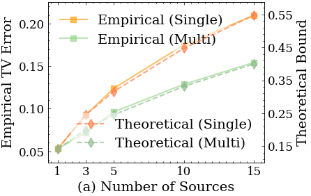
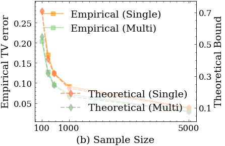
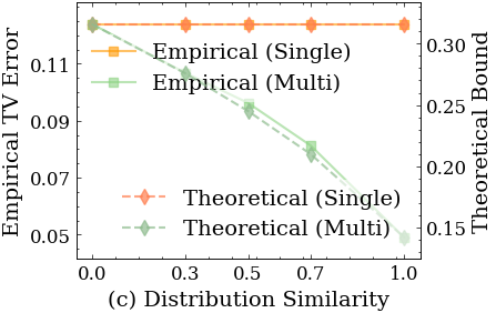
Figure 1: Simulation results for conditional Gaussian estimation. Empirical values (solid lines) correspond to the left vertical axis, while theoretical values (dashed lines) correspond to the right. Single-source results are shown in orange, and multi-source results in green. The matched orders of empirical errors and theoretical upper bounds support the validity of results in Section 4.1.

5 Experiments

In this section, simulations and real-world experiments are conducted to verify our theoretical results in Section 3 and 4.

5.1 Simulations on conditional Gaussian estimation

In this part, we aim to examine the tightness of the derived upper bound that ${\mathcal{R}}_{\overline{\mathrm{TV}}}(\hat{p}_{X|Y}^{\mathrm{multi}})=\tilde{{\mathcal{O}}}(\sqrt{\frac{(K-1)d_{1}+d}{n}})$ in Theorem 4.1 and ${\mathcal{R}}_{\overline{\mathrm{TV}}}(\hat{p}_{X|Y}^{\mathrm{single}})=\tilde{{\mathcal{O}}}(\sqrt{\frac{Kd}{n}})$ in Theorem B.2.

The number of sources $K$, sample size $n$, and the similarity factor $\beta_{\mathrm{sim}}\in[0,1]$ are key parameters. In all of our simulations, we fix data dimension $d=10$ and $p_{Y}^{*}(k)={1}/{K}$ all $k\in[K]$. The dissimilar dimension $d_{1}=d-\lfloor\beta_{\mathrm{sim}}d\rfloor$. We set the source-specific feature as $\phi_{k}=k{\bm{1}}\in\mathbb{R}^{d_{1}}$ and the shared feature as $\psi={\bm{0}}\in\mathbb{R}^{d-d_{1}}$. Under the setting of Section 4.1, conditional MLE has analytical solutions: under multi-source training, we have

$$\textstyle{\hat{\phi}_{k}={\sum_{y_{i}=k}{\bm{x}}_{i}[1\mathrel{\mathop{\ordinarycolon}}d_{1}]}/{n_{k}},\ \hat{\psi}={\sum_{i=1}^{n}{\bm{x}}_{i}[d_{1}+1\mathrel{\mathop{\ordinarycolon}}d]}/{n}},$$

and under single-source training, we have

$$\textstyle{\hat{\phi}_{k}\!=\!{\sum_{y_{i}=k}{\bm{x}}_{i}[1\!\mathrel{\mathop{\ordinarycolon}}\!d_{1}]}/{n_{k}},\ \hat{\psi}_{k}\!=\!{\sum_{y_{i}=k}{\bm{x}}_{i}[d_{1}+1\!\mathrel{\mathop{\ordinarycolon}}\!d]}/{n_{k}}}.$$

For evaluation, we randomly sample $n^{\mathrm{test}}=500$ data points according to the true joint distribution $p^{*}_{X,Y}$. Empirically, we approximate the true TV distance by using the Monte Carlo method based on the test set, which can be written formally as

$${\mathcal{R}}_{\overline{\mathrm{TV}}}(\hat{p}_{X|Y}\!)\!\approx\!\frac{1}{2n^{\mathrm{test}}}\!\sum_{i=1}^{n^{\mathrm{test}}}\left\lvert\frac{\hat{p}_{X|Y}({\bm{x}}_{i}|y_{i})}{p^{*}_{X|Y}({\bm{x}}_{i}|y_{i})}\!-\!1\right\rvert\!=\!{\mathcal{R}}_{\overline{\mathrm{TV}}}^{\mathrm{em}}(\hat{p}_{X|Y}\!).$$

To eliminate the randomness, we average over 5 random runs for each simulation and report the mean results.

Order of the average TV error about $K$.

We range the number of sources $K$ in $[1,3,5,10,15]$ with fixed sample size $n=500$ and similarity factor $\beta_{\mathrm{sim}}=0.5$. We display the empirical average TV error for each $K$ in Figure 1(a), with ${\mathcal{R}}_{\overline{\mathrm{TV}}}^{\mathrm{em}}(\hat{p}_{X|Y}^{\mathrm{multi}})$ colored in green and ${\mathcal{R}}_{\overline{\mathrm{TV}}}^{\mathrm{em}}(\hat{p}_{X|Y}^{\mathrm{single}})$ colored in orange. Ignoring the influence of constants, it shows a good alignment between empirical errors (in solid lines) and theoretical upper bounds (in dashed lines), both scaling as $\tilde{{\mathcal{O}}}(\sqrt{K})$.

Order of the average TV error about $n$.

We range sample size $n$ in $[100,300,500,1000,5000]$ with fixed number of sources $K=5$ and similarity factor $\beta_{\mathrm{sim}}=0.5$. We display the empirical error for each $n$ in Figure 1(b), with ${\mathcal{R}}_{\overline{\mathrm{TV}}}^{\mathrm{em}}(\hat{p}_{X|Y}^{\mathrm{multi}}\!)$ colored in green and ${\mathcal{R}}_{\overline{\mathrm{TV}}}^{\mathrm{em}}(\hat{p}_{X|Y}^{\mathrm{single}}\!)$ colored in orange. Ignoring the influence of constants, it shows that the orders of empirical error about $n$ match well with the theoretical upper bounds which scale as $\tilde{{\mathcal{O}}}(1/\sqrt{n})$.

Order of the average TV error about $\beta_{\mathrm{sim}}$.

We range similarity factor $\beta_{\mathrm{sim}}$ in $[0,0.3,0.5,0.7,1]$ with fixed sample size $n=500$ and number of data sources $K=5$. We display the empirical average TV error for each $\beta_{\mathrm{sim}}$ in Figure 1(c) to observe how similarity factor $\beta_{\mathrm{sim}}$ impacts the advantage of multi-source training. Concretely, as predicted by the theoretical bounds, the changing of $\beta_{\mathrm{sim}}$ will not influence the performance of single-source training but will decrease the error of multi-source training in the order of $\tilde{{\mathcal{O}}}(\sqrt{d_{1}})=\tilde{{\mathcal{O}}}(\sqrt{1-\beta_{\mathrm{sim}}})$. The results show that the theoretical bounds predict the empirical performance well.

To sum up, our simulations verify the validity of our theoretical bounds in Section 4.1. Moreover, in all experiments, ${\mathcal{R}}_{\overline{\mathrm{TV}}}^{\mathrm{em}}(\hat{p}_{X|Y}^{\mathrm{multi}})$ is consistently smaller than ${\mathcal{R}}_{\overline{\mathrm{TV}}}^{\mathrm{em}}(\hat{p}_{X|Y}^{\mathrm{single}})$, supporting our results in Section 3

5.2 Real-world experiments on diffusion models

In this section, we conduct experiments on diffusion models to validate our theoretical findings in real-world scenarios from two aspects: (1) We empirically compare multi-source and single-source training on conditional diffusion models and evaluate their performance to validate the guaranteed advantage of multi-source training against single-source training proved in Section 3. (2) We investigate the trend of this advantage about key factors—the number of sources and distribution similarity—as discussed in Section 4.

Experimental settings.

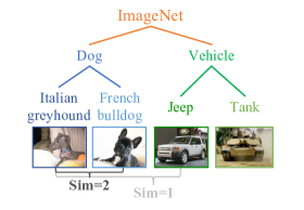
Figure 3: Similarity level.

We train class-conditional diffusion models following EDM2 (Karras et al., 2024) at 256$\times$256 resolution on the selected classes from the ILSVRC2012 training set (Russakovsky et al., 2015), which is a subset of ImageNet (Deng et al., 2009) containing 1.28M natural images from 1000 classes, each annotated with an integer class label from 1 to 1000. In our experiments, we treat each class as a distinct data source. To control similarity among data sources, we manually design two levels of distribution similarity based on the semantic hierarchy of ImageNet (Deng et al., 2010; Bostock., 2018) as shown in Figure 3 in Appendix E along with other experimental details.

For each controlled experiment comparing multi-source and single-source training, we fix $K$ target classes within one similarity level $\mathrm{Sim}$ and train the models on a dataset $S$ consisting of $N$ examples per class. Under multi-source training, we train a single conditional diffusion model for all $K$ classes jointly. Under single-source training, we train $K$ separate conditional diffusion models, one for each class. Please refer to Section 2 for the formal formulation of these two strategies. We set each factor with two possible values: the number of classes $K$ in 3 or 10, distribution similarity $\mathrm{Sim}$ in 1 or 2, and the sample size per class $N$ in 500 or 1000. This results in a total of 8 sets of experiments comparing multi-source and single-source training.

We evaluate model performance using the average Fréchet Inception Distance (Heusel et al., 2017) (FID, a widely used metric for image generation quality) across all conditions to assess the overall conditional generation performance. Results are displayed in Table 1. Specifically, for multi-source training, we compute the FID for each class and take the average over all $K$ classes. For single-source training, we compute the FID for each of the $K$ separately trained models on their respective classes and calculate the average. Relative advantage of multi-source training is measured by $\frac{\text{Avg. FID (Single)}-\text{Avg. FID (Multi)}}{\text{Avg. FID (Single)}}$ as displayed in Figure 2.

Experimental results

In the following, we interpret the results sequentially from the view of our theoretical findings.

From Table 1, we observe that under different amounts of classes $K$, similarity level $\mathrm{Sim}$, and per-class sample size $N$, multi-source training generally achieves lower average FID than that of single-source training, which is consistent with our theoretical guarantees derived in Section 3,

From Figure 2, we observe that for any fixed similarity level $\mathrm{Sim}$ and per-class sample size $N$, the relative advantage of multi-sources training with a larger $K$ (the green bars) is larger than that with a smaller $K$ (the nearby orange bars). Additionally, for any fixed $K$ and $N$, the relative advantage of multi-sources training with a larger distribution similarity is larger than that with a smaller distribution similarity (as shown through the dashed lines). These results support our theoretical insights in Section 4 that the number of sources and similarity among source distributions improves the advantage of multi-source training.

Table 1: Average FID for single-source and multi-source training. Under different amounts of classes $K$, similarity level $\mathrm{Sim}$, and per-class sample size $N$, multi-source training generally achieves lower average FID than that of single-source training, which is consistent with our theoretical guarantees derived in Section 3.

$N$	$\mathrm{Sim}$	$K$	Avg. FID $\downarrow$ (Single)	Avg. FID $\downarrow$ (Multi)
500	1	3	30.15	29.82
		10	30.16	29.36
	2	3	32.87	31.16
		10	29.96	28.83
1000	1	3	27.76	26.86
		10	27.46	25.01
	2	3	30.20	28.31
		10	29.60	26.70

6 Other related works

Distribution estimation guarantee for MLE.

Classical approaches investigate distribution estimation for MLE in Hellinger distance based on the bracketing number and the uniform law of large numbers from empirical process theory (Wong & Shen, 1995; Geer, 2000), which yields high-probability bounds of similar order as Theorem 3.2. Ge et al. (2024) extend the analysis to derive TV error bound under the realizable assumption. We further adapt their techniques to conditional generative modeling by introducing the upper bracketing number to quantify the complexity of conditional distribution space in Definition 3.1 and modify the proofs to handle conditional MLE in Section A.1.

Theory on multi-task learning.

Multi-task learning is a well-studied topic in supervised learning (Caruana, 1997; Baxter, 2000). It typically benefits from similarities across tasks, sharing some commonality with multi-source training. However, theoretical analyses in supervised learning often assume a bounded objective (Ben-David & Borbely, 2008; Maurer et al., 2016; Tripuraneni et al., 2020), whereas our MLE analysis imposes no such restriction.

Advanced theory on generative models.

Among generative models based on (approximate) MLE (LeCun et al., 2006; Uria et al., 2016; Ho et al., 2020), diffusion models have been extensively studied theoretically on its score approximation, sampling behavior, and distribution estimation (Oko et al., 2023; Chen et al., 2023a, b; Fu et al., 2024). This paper focuses on distribution estimation for general conditional generative modeling. Incorporating existing literature could be a promising direction for future work.

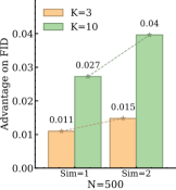
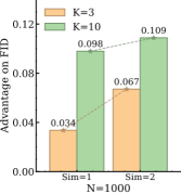
Figure 2: Relative advantage of multi-source training. For any fixed similarity level $\mathrm{Sim}$ and per-class sample size $N$, a larger $K$ yields a greater FID improvement than a smaller $K$. For any fixed $K$ and $N$, higher distribution similarity leads to greater FID improvement (illustrated by dashed lines). These results support the theoretical findings in Section 4.

7 Conclusion and discussion

This paper provides the first attempt to rigorously analyze the conditional generative modeling on multiple data sources from a distribution estimation perspective. In particular, we establish a general estimation error bound in average TV distance under the realizable assumption based on the bracketing number of the conditional distribution space. When source distributions share parametric similarities, multi-source training has a provable advantage against single-source training by reducing the bracketing number. We further instantiate the general theory on three specific models to obtain concrete error bounds. To achieve this, novel bracketing number bounds for ARMs and EBMs are established. The results show that the number of data sources and the similarity between source distributions enhance the benefits of multi-source training. Simulations and real-world experiments support our theoretical findings.

Our theoretical setting differs from practice in some aspects, e.g., language models have no explicit conditions, and image generation models are commonly conditioned on descriptive text involving multiple conditions. However, our abstraction provides a simplified framework that preserves the core properties of multi-source training and isolates how individual source distributions are learned. Moreover, recent studies suggest adding source labels, such as domain names, at the start of training text for language models can enhance performance (Allen-Zhu & Li, 2024b; Gao et al., 2025), which may become a standard practice in the future.

Impact Statement

This paper presents work whose goal is to advance the field of Machine Learning. There are many potential societal consequences of our work, none of which we feel must be specifically highlighted here.

Appendix A Proofs for Section 3

A.1 Proof of Theorem 3.2

Proof of Theorem 3.2.

This theorem applies to both discrete and continuous random variables, while we use integration notation in the proof for generality. In the following, we first present an elementary inequality (in Equation 10) which serves as a toolkit for the subsequent derivations. Then we decompose the TV distance and derive its complexity-based upper bound (in Equation 12) using the former inequality. Finally, after specifying certain constants in this upper bound, a clearer order w.r.t. $n$ is revealed (in Equation 13).

Intermediate result induced by union bound.

Let $\epsilon$ be a real number that $\epsilon>0$ and $\mathsf{p}$ be an integer that $1\leq\mathsf{p}\leq\infty$. Let ${\mathcal{B}}$ be an $\epsilon$-upper bracket of ${\mathcal{P}}_{X|Y}$ w.r.t. $L^{1}({\mathscr{X}})$ such that $\lvert{\mathcal{B}}\rvert={\mathcal{N}}_{[]}\left(\epsilon;{\mathcal{P}}_{X|Y},L^{1}({\mathscr{X}})\right)$.

According to the minimum cardinality requirement, we obtain a proposition of ${\mathcal{B}}$ that: for any $p^{\prime}\in{\mathcal{B}}$, $p^{\prime}({\bm{x}},y)\geq 0$ on ${\mathscr{X}}\times{\mathscr{Y}}$. Let’s first consider $\prod_{i=1}^{n}\sqrt{\frac{p^{\prime}({\bm{x}}_{i},y_{i})}{p^{*}_{X|Y}({\bm{x}}_{i}|y_{i})}}$ as a random variable on $S$, where we suppose $p^{*}_{X,Y}({\bm{x}}_{i},y_{i})>0$ since $({\bm{x}}_{i},y_{i})$ are sampled from $p^{*}_{X,Y}$ and thus $p^{*}_{X|Y}({\bm{x}}_{i}|y_{i})\neq 0$. By applying the Markov inequality, we have: given any $0<\delta^{\prime}<1$,

$${\mathrm{Pr}}_{S}\left(\prod_{i=1}^{n}\sqrt{\frac{p^{\prime}({\bm{x}}_{i},y_{i})}{p^{*}_{X|Y}({\bm{x}}_{i}|y_{i})}}\geq\frac{1}{\delta^{\prime}}\mathbb{E}_{S}\left[\prod_{i=1}^{n}\sqrt{\frac{p^{\prime}({\bm{x}}_{i},y_{i})}{p^{*}_{X|Y}({\bm{x}}_{i}|y_{i})}}\right]\right)\leq\delta^{\prime}.$$ (8)

Applying the union bound on all $p^{\prime}\in{\mathcal{B}}$, we further have:

$${\mathrm{Pr}}_{S}\left(\forall p^{\prime}\in{\mathcal{B}},\prod_{i=1}^{n}\sqrt{\frac{p^{\prime}({\bm{x}}_{i},y_{i})}{p^{*}_{X|Y}({\bm{x}}_{i}|y_{i})}}<\frac{1}{\delta^{\prime}}\mathbb{E}_{S}\left[\prod_{i=1}^{n}\sqrt{\frac{p^{\prime}({\bm{x}}_{i},y_{i})}{p^{*}_{X|Y}({\bm{x}}_{i}|y_{i})}}\right]\right)$$

$$= 1-{\mathrm{Pr}}_{S}\left(\exists p^{\prime}\in{\mathcal{B}},\prod_{i=1}^{n}\sqrt{\frac{p^{\prime}({\bm{x}}_{i},y_{i})}{p^{*}_{X|Y}({\bm{x}}_{i}|y_{i})}}\geq\frac{1}{\delta^{\prime}}\mathbb{E}_{S}\left[\prod_{i=1}^{n}\sqrt{\frac{p^{\prime}({\bm{x}}_{i},y_{i})}{p^{*}_{X|Y}({\bm{x}}_{i}|y_{i})}}\right]\right)$$

$$= 1-{\mathrm{Pr}}_{S}\left(\bigcup_{p^{\prime}\in{\mathcal{B}}}\left\{\prod_{i=1}^{n}\sqrt{\frac{p^{\prime}({\bm{x}}_{i},y_{i})}{p^{*}_{X|Y}({\bm{x}}_{i}|y_{i})}}\geq\frac{1}{\delta^{\prime}}\mathbb{E}_{S}\left[\prod_{i=1}^{n}\sqrt{\frac{p^{\prime}({\bm{x}}_{i},y_{i})}{p^{*}_{X|Y}({\bm{x}}_{i}|y_{i})}}\right]\right\}\right)$$

$$\geq 1-\sum_{p^{\prime}\in{\mathcal{B}}}{\mathrm{Pr}}_{S}\left(\prod_{i=1}^{n}\sqrt{\frac{p^{\prime}({\bm{x}}_{i},y_{i})}{p^{*}_{X|Y}({\bm{x}}_{i}|y_{i})}}\geq\frac{1}{\delta^{\prime}}\mathbb{E}_{S}\left[\prod_{i=1}^{n}\sqrt{\frac{p^{\prime}({\bm{x}}_{i},y_{i})}{p^{*}_{X|Y}({\bm{x}}_{i}|y_{i})}}\right]\right)$$ (by union bound)

$$\geq 1-{\mathcal{N}}_{[]}\left(\epsilon;{\mathcal{P}}_{X|Y},L^{1}({\mathscr{X}})\right)\delta^{\prime}.$$ (by Equation 8)

By denoting that $\delta\coloneqq{\mathcal{N}}_{[]}\left(\epsilon;{\mathcal{P}}_{X|Y},L^{1}({\mathscr{X}})\right)\delta^{\prime}$, we have: it holds with probability at least $1-\delta$ that for all $p^{\prime}\in{\mathcal{B}}$,

$$\prod_{i=1}^{n}\sqrt{\frac{p^{\prime}({\bm{x}}_{i},y_{i})}{p^{*}_{X|Y}({\bm{x}}_{i}|y_{i})}}<\frac{{\mathcal{N}}_{[]}\left(\epsilon;{\mathcal{P}}_{X|Y},L^{1}({\mathscr{X}})\right)}{\delta}\mathbb{E}_{S}\left[\prod_{i=1}^{n}\sqrt{\frac{p^{\prime}({\bm{x}}_{i},y_{i})}{p^{*}_{X|Y}({\bm{x}}_{i}|y_{i})}}\right].$$

Taking logarithms at both sides, we have

$$\frac{1}{2}\sum_{i=1}^{n}\log\frac{p^{\prime}({\bm{x}}_{i},y_{i})}{p^{*}_{X|Y}({\bm{x}}_{i}|y_{i})} \leq\log\mathbb{E}_{S}\left[\prod_{i=1}^{n}\sqrt{\frac{p^{\prime}({\bm{x}}_{i},y_{i})}{p^{*}_{X|Y}({\bm{x}}_{i}|y_{i})}}\right]+\log\frac{{\mathcal{N}}_{[]}\left(\epsilon;{\mathcal{P}}_{X|Y},L^{1}({\mathscr{X}})\right)}{\delta}$$

$$=\log\prod_{i=1}^{n}\mathbb{E}_{({\bm{x}}_{i},y_{i})\sim p^{*}_{X,Y}}\left[\sqrt{\frac{p^{\prime}({\bm{x}}_{i},y_{i})}{p^{*}_{X|Y}({\bm{x}}_{i}|y_{i})}}\right]+\log\frac{{\mathcal{N}}_{[]}\left(\epsilon;{\mathcal{P}}_{X|Y},L^{1}({\mathscr{X}})\right)}{\delta} \{x_{i}\}_{i=1}^{n} p^{*}_{X}$$ ( are i.i.d. sampled from )

$$=n\log\mathbb{E}_{X,Y}\left[\sqrt{\frac{p^{\prime}({\bm{x}},y)}{p^{*}_{X|Y}({\bm{x}}|y)}}\right]+\log\frac{{\mathcal{N}}_{[]}\left(\epsilon;{\mathcal{P}}_{X|Y},L^{1}({\mathscr{X}})\right)}{\delta}$$

$$=n\log\mathbb{E}_{Y}\left[\mathbb{E}_{X|Y}\left[\sqrt{\frac{p^{\prime}({\bm{x}},y)}{p^{*}_{X|Y}({\bm{x}}|y)}}\right]\right]+\log\frac{{\mathcal{N}}_{[]}\left(\epsilon;{\mathcal{P}}_{X|Y},L^{1}({\mathscr{X}})\right)}{\delta}$$

$$=n\log\mathbb{E}_{Y}\left[\int_{{\mathscr{X}}}p^{*}_{X|Y}({\bm{x}}|y)\sqrt{\frac{p^{\prime}({\bm{x}},y)}{p^{*}_{X|Y}({\bm{x}}|y)}}d{\bm{x}}\right]+\log\frac{{\mathcal{N}}_{[]}\left(\epsilon;{\mathcal{P}}_{X|Y},L^{1}({\mathscr{X}})\right)}{\delta}$$

$$=n\log\mathbb{E}_{Y}\left[\int_{{\mathscr{X}}}\sqrt{p^{\prime}({\bm{x}},y)p^{*}_{X|Y}({\bm{x}}|y)}d{\bm{x}}\right]+\log\frac{{\mathcal{N}}_{[]}\left(\epsilon;{\mathcal{P}}_{X|Y},L^{1}({\mathscr{X}})\right)}{\delta}.$$

As $\log x\leq x-1$ for all $x>0$, the inequality can be further transformed into

$$\frac{1}{2}\sum_{i=1}^{n}\log\frac{p^{\prime}({\bm{x}}_{i},y_{i})}{p^{*}_{X|Y}({\bm{x}}_{i}|y_{i})}\leq n\left(\mathbb{E}_{Y}\left[\int_{{\mathscr{X}}}\sqrt{p^{\prime}({\bm{x}},y)p^{*}_{X|Y}({\bm{x}}|y)}d{\bm{x}}\right]-1\right)+\log\frac{{\mathcal{N}}_{[]}\left(\epsilon;{\mathcal{P}}_{X|Y},L^{1}({\mathscr{X}})\right)}{\delta}.$$ (9)

Elementary inequality for MLE estimators.

Since the real conditional distribution $p^{*}_{X|Y}$ is in ${\mathcal{P}}_{X|Y}$, for the likelihood maximizers $\hat{p}_{X|Y}\in{\mathcal{P}}_{X|Y}$, we have $L_{S}(\hat{p}_{X|Y})=\prod_{i=1}^{n}\hat{p}_{X|Y}({\bm{x}}_{i}|y_{i})\geq L_{S}(p^{*}_{X|Y})=\prod_{i=1}^{n}p^{*}_{X|Y}({\bm{x}}_{i}|y_{i})$, and thus $\frac{1}{2}\sum_{i=1}^{n}\log\frac{\hat{p}_{X|Y}({\bm{x}}_{i}|y_{i})}{p^{*}_{X|Y}({\bm{x}}_{i}|y_{i})}=\frac{1}{2}\log\frac{\prod_{i=1}^{n}\hat{p}_{X|Y}({\bm{x}}_{i}|y_{i})}{\prod_{i=1}^{n}p^{*}_{X|Y}({\bm{x}}_{i}|y_{i})}\geq\frac{1}{2}\log 1=0$. According to the definition of upper bracketing number, there exists some $\hat{p}^{\prime}\in{\mathcal{B}}$ such that given any $y\in{\mathscr{Y}}$, it holds that: (i) $\forall x\in{\mathscr{X}},\hat{p}^{\prime}({\bm{x}},y)\geq\hat{p}_{X|Y}({\bm{x}}|y)$, and (ii) $\lVert\hat{p}^{\prime}(\cdot,y)-\hat{p}_{X|Y}(\cdot|y)\rVert_{L^{1}({\mathscr{X}})}=\int_{{\mathscr{X}}}\lvert\hat{p}^{\prime}({\bm{x}},y)-\hat{p}_{X|Y}({\bm{x}}|y)\rvert d{\bm{x}}\leq\epsilon.$ Applying (i), we have:

$$\frac{1}{2}\sum_{i=1}^{n}\log\frac{\hat{p}^{\prime}({\bm{x}}_{i},y_{i})}{p^{*}_{X|Y}({\bm{x}}_{i}|y_{i})}\geq\frac{1}{2}\sum_{i=1}^{n}\log\frac{\hat{p}_{X|Y}({\bm{x}}_{i}|y_{i})}{p^{*}_{X|Y}({\bm{x}}_{i}|y_{i})}\geq 0.$$

Combining this with Equation 9 and rearranging the terms, we have: it holds with at least probability $1-\delta$ that

$$1-\mathbb{E}_{Y}\left[\int_{{\mathscr{X}}}\sqrt{p^{\prime}({\bm{x}},y)p^{*}_{X|Y}({\bm{x}}|y)}d{\bm{x}}\right]\leq\frac{1}{n}\log\frac{{\mathcal{N}}_{[]}\left(\epsilon;{\mathcal{P}}_{X|Y},L^{1}({\mathscr{X}})\right)}{\delta}.$$ (10)

This serves as an elementary toolkit for deriving the subsequent upper bounds.

Decomposing the square of the TV distance.

Recalling that $\mathrm{TV}(\hat{p}_{X|Y},p^{*}_{X|Y})=\frac{1}{2}\int_{{\mathscr{X}}}\lvert\hat{p}_{X|Y}({\bm{x}}|y)-p^{*}_{X|Y}({\bm{x}}|y)\rvert d{\bm{x}}$, we will decompose its square and then bound each term sequentially. First, we use the above $\hat{p}^{\prime}({\bm{x}},y)$ as an intermediate term to decompose the square of $2\mathrm{TV}(\hat{p}_{X|Y},p^{*}_{X|Y})$ into parts that can be effectively upper bounded:

$$\left(2\mathrm{TV}(\hat{p}_{X|Y},p^{*}_{X|Y})\right)^{2}=\left(\int_{{\mathscr{X}}}\lvert\hat{p}_{X|Y}({\bm{x}}|y)-p^{*}_{X|Y}({\bm{x}}|y)\rvert d{\bm{x}}\right)^{2}$$

$$= \underbrace{\left(\int_{{\mathscr{X}}}\lvert\hat{p}_{X|Y}({\bm{x}}|y)-p^{*}_{X|Y}({\bm{x}}|y)\rvert d{\bm{x}}\right)^{2}-\left(\int_{{\mathscr{X}}}\lvert\hat{p}^{\prime}({\bm{x}},y)-p^{*}_{X|Y}({\bm{x}}|y)\rvert d{\bm{x}}\right)^{2}}_{\text{(I)}}+\underbrace{\left(\int_{{\mathscr{X}}}\lvert\hat{p}^{\prime}({\bm{x}},y)-p^{*}_{X|Y}({\bm{x}}|y)\rvert d{\bm{x}}\right)^{2}}_{\text{(II)}}.$$

For (I), we have

$$\left(\int_{{\mathscr{X}}}\lvert\hat{p}_{X|Y}({\bm{x}}|y)-p^{*}_{X|Y}({\bm{x}}|y)\rvert d{\bm{x}}\right)^{2}-\left(\int_{{\mathscr{X}}}\lvert\hat{p}^{\prime}({\bm{x}},y)-p^{*}_{X|Y}({\bm{x}}|y)\rvert d{\bm{x}}\right)^{2}$$

$$= \left(\int_{{\mathscr{X}}}\lvert\hat{p}_{X|Y}({\bm{x}}|y)-p^{*}_{X|Y}({\bm{x}}|y)\rvert+\lvert\hat{p}^{\prime}({\bm{x}},y)-p^{*}_{X|Y}({\bm{x}}|y)\rvert d{\bm{x}}\right)\left(\int_{{\mathscr{X}}}\lvert\hat{p}_{X|Y}({\bm{x}}|y)-p^{*}_{X|Y}({\bm{x}}|y)\rvert-\lvert\hat{p}^{\prime}({\bm{x}},y)-p^{*}_{X|Y}({\bm{x}}|y)\rvert d{\bm{x}}\right)$$

$$\leq \left(\int_{{\mathscr{X}}}\lvert\hat{p}_{X|Y}({\bm{x}}|y)\rvert+\lvert p^{*}_{X|Y}({\bm{x}}|y)\rvert+\lvert\hat{p}^{\prime}({\bm{x}},y)-\hat{p}_{X|Y}({\bm{x}}|y)\rvert+\lvert\hat{p}_{X|Y}({\bm{x}}|y)\rvert+\lvert p^{*}_{X|Y}({\bm{x}}|y)\rvert d{\bm{x}}\right)\left(\int_{{\mathscr{X}}}\lvert\hat{p}_{X|Y}({\bm{x}}|y)-\hat{p}^{\prime}({\bm{x}},y)\rvert d{\bm{x}}\right)$$

$$\leq (\epsilon+4)\epsilon.$$

The first inequality holds for the triangle inequality $\lvert a+b\rvert\leq\lvert a\rvert+\lvert b\rvert$ and the reverse triangle inequality $\lvert\lvert a\rvert-\lvert b\rvert\rvert\leq\lvert a-b\rvert$. The second inequality holds for the normalization property of conditional distributions ($\int_{{\mathscr{X}}}\lvert\hat{p}_{X|Y}({\bm{x}}|y)\rvert d{\bm{x}}$ and $\int_{{\mathscr{X}}}\lvert p^{*}_{X|Y}({\bm{x}}|y)\rvert d{\bm{x}}$ equal $1$) and the property of the $\epsilon$-upper bracket ($\int_{{\mathscr{X}}}\lvert\hat{p}^{\prime}({\bm{x}},y)-\hat{p}_{X|Y}({\bm{x}}|y)\rvert d{\bm{x}}\leq\epsilon$).

For (II), we have

$$\left(\int_{{\mathscr{X}}}\lvert\hat{p}^{\prime}({\bm{x}},y)-p^{*}_{X|Y}({\bm{x}}|y)\rvert d{\bm{x}}\right)^{2}$$

$$\leq \left(\int_{{\mathscr{X}}}\left(\sqrt{\hat{p}^{\prime}({\bm{x}},y)}+\sqrt{p^{*}_{X|Y}({\bm{x}}|y)}\right)^{2}dx\right)\left(\int_{{\mathscr{X}}}\left(\sqrt{\hat{p}^{\prime}({\bm{x}},y)}-\sqrt{p^{*}_{X|Y}({\bm{x}}|y)}\right)^{2}dx\right)$$ (by Cauchy–Schwarz inequality)

$$\leq \left(\int_{{\mathscr{X}}}2\left(\hat{p}^{\prime}({\bm{x}},y)+p^{*}_{X|Y}({\bm{x}}|y)\right)d{\bm{x}}\right)\left(\int_{{\mathscr{X}}}{\hat{p}^{\prime}({\bm{x}},y)+p^{*}_{X|Y}({\bm{x}}|y)-2\sqrt{\hat{p}^{\prime}({\bm{x}},y)p^{*}_{X|Y}({\bm{x}}|y)}}d{\bm{x}}\right) (a+b)^{2}\leq 2(a^{2}+b^{2})$$ (by )

$$= 2\left(\int_{{\mathscr{X}}}{\hat{p}^{\prime}({\bm{x}},y)-\hat{p}_{X|Y}({\bm{x}}|y)+\hat{p}_{X|Y}({\bm{x}}|y)+p^{*}_{X|Y}({\bm{x}}|y)}d{\bm{x}}\right)$$

$$\left(\int_{{\mathscr{X}}}{\hat{p}^{\prime}({\bm{x}},y)-\hat{p}_{X|Y}({\bm{x}}|y)+\hat{p}_{X|Y}({\bm{x}}|y)+p^{*}_{X|Y}({\bm{x}}|y)-2\sqrt{\hat{p}^{\prime}({\bm{x}},y)p^{*}_{X|Y}({\bm{x}}|y)}}d{\bm{x}}\right)$$

$$\leq 2(\epsilon+2)\left(\epsilon+2-2\int_{{\mathscr{X}}}\sqrt{\hat{p}^{\prime}({\bm{x}},y)p^{*}_{X|Y}({\bm{x}}|y)}d{\bm{x}}\right). \int_{{\mathscr{X}}}\lvert\hat{p}_{X|Y}({\bm{x}}|y)\rvert d{\bm{x}}=\int_{{\mathscr{X}}}\lvert p^{*}_{X|Y}({\bm{x}}|y)\rvert d{\bm{x}}=1 \int_{{\mathscr{X}}}\lvert\hat{p}^{\prime}({\bm{x}},y)-\hat{p}_{X|Y}({\bm{x}}|y)\rvert d{\bm{x}}\leq\epsilon$$ (by and )

Putting together (I) and (II), we get:

$$\mathrm{TV}(\hat{p}_{X|Y},p^{*}_{X|Y}) =\frac{1}{2}\sqrt{\left(\int_{{\mathscr{X}}}\lvert\hat{p}_{X|Y}({\bm{x}}|y)-p^{*}_{X|Y}({\bm{x}}|y)\rvert d{\bm{x}}\right)^{2}}$$

$$\leq\frac{1}{2}\sqrt{(\epsilon+4)\epsilon+2(\epsilon+2)\left(\epsilon+2-2\int_{{\mathscr{X}}}\sqrt{\hat{p}^{\prime}({\bm{x}},y)p^{*}_{X|Y}({\bm{x}}|y)}d{\bm{x}}\right)}.$$ (11)

Bounding the average TV error.

Based on the above results, we upper bound the average TV error (defined in Equation 4) of $\hat{p}_{X|Y}$ as follows:

$${\mathcal{R}}_{\overline{\mathrm{TV}}}(\hat{p}_{X|Y})= \mathbb{E}_{Y}\left[\mathrm{TV}(\hat{p}_{X|Y},p^{*}_{X|Y})\right]$$

$$\leq \frac{1}{2}\mathbb{E}_{Y}\left[\sqrt{(\epsilon+4)\epsilon+2(\epsilon+2)\left(\epsilon+2-2\int_{{\mathscr{X}}}\sqrt{\hat{p}^{\prime}({\bm{x}},y)p^{*}_{X|Y}({\bm{x}}|y)}d{\bm{x}}\right)}\right]$$ (by Section A.1)

$$\leq \frac{1}{2}\sqrt{\mathbb{E}_{Y}\left[(\epsilon+4)\epsilon+2(\epsilon+2)\left(\epsilon+2-2\int_{{\mathscr{X}}}\sqrt{\hat{p}^{\prime}({\bm{x}},y)p^{*}_{X|Y}({\bm{x}}|y)}d{\bm{x}}\right)\right]} f(x)=\sqrt{x}$$ (by concavity of and Jensen’s inequality)

$$= \frac{1}{2}\sqrt{(\epsilon+4)\epsilon+2(\epsilon+2)\left(\epsilon+2\left(1-\mathbb{E}_{Y}\left[\int_{{\mathscr{X}}}\sqrt{\hat{p}^{\prime}({\bm{x}},y)p^{*}_{X|Y}({\bm{x}}|y)}d{\bm{x}}\right]\right)\right)}.$$ (by the linearity of expectation)

Recalling the elementary inequality we derived formerly in Equation 10, we have: it holds with at least probability $1-\delta$ that

$${\mathcal{R}}_{\overline{\mathrm{TV}}}(\hat{p}_{X|Y})\leq\frac{1}{2}\sqrt{(\epsilon+4)\epsilon+2(\epsilon+2)\left(\epsilon+\frac{2}{n}\log\frac{{\mathcal{N}}_{[]}\left(\epsilon;{\mathcal{P}}_{X|Y},L^{1}({\mathscr{X}})\right)}{\delta}\right)}.$$ (12)

Recalling that $0\leq\delta\leq\frac{1}{2}$ and for non-empty ${\mathcal{P}}_{X|Y}$, ${\mathcal{N}}_{[]}\left(\epsilon;{\mathcal{P}}_{X|Y},L^{1}({\mathscr{X}})\right)\geq 1$, we have ${\mathcal{N}}_{[]}\left(\epsilon;{\mathcal{P}}_{X|Y},L^{1}({\mathscr{X}})\right)/\delta\geq 2\geq e^{\frac{1}{2}}$. Taking $\epsilon=1/n$ in Equation 12, it then holds with probability at least $1-\delta$ that

$${\mathcal{R}}_{\overline{\mathrm{TV}}}(\hat{p}_{X|Y}) \leq\frac{1}{2}\sqrt{(\frac{1}{n}+4)\frac{1}{n}+2(\frac{1}{n}+2)\left(\frac{1}{n}+\frac{2}{n}\log\frac{{\mathcal{N}}_{[]}\left(\frac{1}{n};{\mathcal{P}}_{X|Y},L^{1}({\mathscr{X}})\right)}{\delta}\right)}$$

$$\leq\frac{1}{2}\sqrt{\frac{5}{n}+6\left(\frac{1}{n}+\frac{2}{n}\log\frac{{\mathcal{N}}_{[]}\left(\frac{1}{n};{\mathcal{P}}_{X|Y},L^{1}({\mathscr{X}})\right)}{\delta}\right)} \frac{1}{n}\leq 1$$ (by )

$$\leq\frac{1}{2}\sqrt{\frac{10}{n}\log\frac{{\mathcal{N}}_{[]}\left(\frac{1}{n};{\mathcal{P}}_{X|Y},L^{1}({\mathscr{X}})\right)}{\delta}+6\left(\frac{4}{n}\log\frac{{\mathcal{N}}_{[]}\left(\frac{1}{n};{\mathcal{P}}_{X|Y},L^{1}({\mathscr{X}})\right)}{\delta}\right)} \frac{1}{n}\leq\frac{2}{n}\log\frac{{\mathcal{N}}_{[]}\left(\frac{1}{n};{\mathcal{P}}_{X|Y},L^{1}({\mathscr{X}})\right)}{\delta}$$ (by )

$$=\frac{1}{2}\sqrt{\frac{34}{n}\log\frac{{\mathcal{N}}_{[]}\left(\frac{1}{n};{\mathcal{P}}_{X|Y},L^{1}({\mathscr{X}})\right)}{\delta}}\leq 3\sqrt{\frac{1}{n}{\log\frac{{\mathcal{N}}_{[]}\left(\frac{1}{n};{\mathcal{P}}_{X|Y},L^{1}({\mathscr{X}})\right)}{\delta}}}$$

$$=3\sqrt{\frac{1}{n}\left(\log{\mathcal{N}}_{[]}\left(\frac{1}{n};{\mathcal{P}}_{X|Y},L^{1}({\mathscr{X}})\right)+\log\frac{1}{\delta}\right)}.$$ (13)

Until now, we have completed the proof of this theorem.

∎

A.2 Proof of Proposition 3.3

Proof of Proposition 3.3.

As defined in Section 2, it holds that ${\mathcal{P}}_{X|Y}^{\mathrm{multi}}\subset{\mathcal{P}}_{X|Y}^{\mathrm{single}}$. Then, for any $p_{X|Y}^{\mathrm{multi}}\in{\mathcal{P}}_{X|Y}^{\mathrm{multi}}$, there exists some $p_{X|Y}^{\mathrm{single}}\in{\mathcal{P}}_{X|Y}^{\mathrm{single}}$ such that $p_{X|Y}^{\mathrm{single}}=p_{X|Y}^{\mathrm{multi}}$. Given any $\epsilon>0$ and $1\leq\mathsf{p}\leq\infty$, let ${\mathcal{B}}^{\mathrm{single}}$ be a $\epsilon$-upper bracket w.r.t. $L^{\mathsf{p}}({\mathscr{X}})$ for ${\mathcal{P}}_{X|Y}^{\mathrm{single}}$ such that $\lvert{\mathcal{B}}^{\mathrm{single}}\rvert={\mathcal{N}}_{[]}\left(\epsilon;{\mathcal{P}}_{X|Y}^{\mathrm{single}},L^{\mathsf{p}}({\mathscr{X}})\right)$. According to the definition of $\epsilon$-upper bracket (as in Definition 3.1), there exists some $p^{\prime}\in{\mathcal{B}}^{\mathrm{single}}$ such that given any $y\in{\mathscr{Y}}$, it holds that: $\forall{\bm{x}}\in{\mathscr{X}},p^{\prime}({\bm{x}},y)\geq p_{X|Y}^{\mathrm{single}}({\bm{x}}|y)=p_{X|Y}^{\mathrm{multi}}({\bm{x}}|y)$, and $\lVert p^{\prime}(\cdot,y)-p_{X|Y}^{\mathrm{multi}}(\cdot|y)\rVert_{L^{\mathsf{p}}({\mathscr{X}})}=\lVert p^{\prime}(\cdot,y)-p_{X|Y}^{\mathrm{single}}(\cdot|y)\rVert_{L^{\mathsf{p}}({\mathscr{X}})}\leq\epsilon.$ Therefore, ${\mathcal{B}}^{\mathrm{single}}$ is also a $\epsilon$-upper bracket w.r.t. $L^{\mathsf{p}}({\mathscr{X}})$ for ${\mathcal{P}}_{X|Y}^{\mathrm{multi}}$, and thus ${\mathcal{N}}_{[]}\left(\epsilon;{\mathcal{P}}_{X|Y}^{\mathrm{multi}},L^{\mathsf{p}}({\mathscr{X}})\right)\leq\lvert{\mathcal{B}}^{\mathrm{single}}\rvert={\mathcal{N}}_{[]}\left(\epsilon;{\mathcal{P}}_{X|Y}^{\mathrm{single}},L^{\mathsf{p}}({\mathscr{X}})\right)$. ∎

Appendix B Proofs for Section 4.1

B.1 Bracketing number of conditional Gaussian distribution space

According to Theorem 3.2, to derive the upper bound of average TV error, we need to measure the upper bracketing number for the conditional Gaussian distribution space. This result mainly follows the bracketing number analysis of Gaussian distribution space in Lemma C.5 in (Ge et al., 2024), and slightly modifies it to conditional Gaussian distribution space.

Theorem B.1 (Bracketing number upper bound for conditional Gaussian distribution space under multi-source training).

Let $B$ be a constant that $0<B<\infty$, suppose that $\Phi=[-B,B]^{d_{1}}$, $\Psi=[-B,B]^{d-d_{1}}$, and conditional distributions in ${\mathcal{P}}_{X|Y}^{\mathrm{multi}}$ are formulated as in Equation 5. Then, given any $0<\epsilon\leq 1$, the $\epsilon$-upper bracketing number of ${\mathcal{P}}_{X|Y}^{\mathrm{multi}}$ w.r.t. $L^{1}({\mathscr{X}})$ satisfies

$${\mathcal{N}}_{[]}\left(\epsilon;{\mathcal{P}}_{X|Y}^{\mathrm{multi}},L^{1}({\mathscr{X}})\right)\leq\left({\frac{2(1+d)B}{\epsilon}}+1\right)^{(K-1)d_{1}+d}.$$

Proof.

According to the assumptions, the conditional distribution space expressed by the parametric estimation model is

$${\mathcal{P}}_{X|Y}^{\mathrm{multi}}\!\coloneqq\!\!\left\{\!p_{X|Y}^{\mathrm{multi}}({\bm{x}}|y)\!=\!\!\prod_{k=1}^{K}\!\left(p_{\phi_{k},\psi}({\bm{x}}|k)\right)^{\mathbb{I}(y=k)}\!=\!\!\prod_{k=1}^{K}\!\left((2\pi)^{-\frac{d}{2}}e^{-\frac{1}{2}\lVert{\bm{x}}-(\phi_{k},\psi)\rVert_{2}^{2}}\right)^{\!\mathbb{I}(y=k)}\!\!\mathrel{\mathop{\ordinarycolon}}\!\phi_{k}\!\in\![-B,B]^{d_{1}},\!\psi\!\in\![-B,B]^{d-d_{1}}\!\right\}.$$

For any $p_{X|Y}^{\mathrm{multi}}({\bm{x}}|y)\!=\!\prod_{k=1}^{K}\left((2\pi)^{-\frac{d}{2}}e^{-\frac{1}{2}\lVert{\bm{x}}-(\phi_{k},\psi)\rVert_{2}^{2}}\right)^{\mathbb{I}(y=k)}\in{\mathcal{P}}_{X|Y}^{\mathrm{multi}}$, let’s first divide the mean vector $(\phi_{k},\psi)$ into $\eta$-width grids with a small constant $\eta>0$ (the value of $\eta$ will be specified later): If $(\phi_{k})_{i}\in[j\eta,(j+1)\eta)$ for some $j\in\mathbb{Z}$, let $(\bar{\phi}_{k})_{i}=j\eta$ and $\bar{\phi}_{k}\coloneqq\left((\bar{\phi}_{k})_{1},\dots,(\bar{\phi}_{k})_{d_{1}}\right)$. Similarly, if $(\psi)_{i}\in[j\eta,(j+1)\eta)$ for some $j\in\mathbb{Z}$, let $(\bar{\psi})_{i}=j\eta$ and $\bar{\psi}\coloneqq\left((\bar{\psi})_{1},\dots,(\bar{\psi})_{d-d_{1}}\right)$. In this case, we have $\lVert(\phi_{k},\psi)-(\bar{\phi}_{k},\bar{\psi})\rVert_{2}^{2}\leq d\eta^{2}$.

Let

$$p^{\prime}({\bm{x}},y)=\prod_{k=1}^{K}\left((2\pi)^{-\frac{d}{2}}e^{-\frac{c_{1}}{2}\lVert{\bm{x}}-(\bar{\phi}_{k},\bar{\psi})\rVert_{2}^{2}+c_{2}}\right)^{\mathbb{I}(y=k)}.$$

According to the definition of the bracketing, we want to prove that $p^{\prime}({\bm{x}},y)\geq p_{X|Y}^{\mathrm{multi}}({\bm{x}}|y)$. By completing the square w.r.t. ${\bm{x}}$, we have

$$-\frac{c_{1}}{2}\lVert{\bm{x}}-(\bar{\phi}_{k},\bar{\psi})\rVert_{2}^{2}+c_{2}-\left(-\frac{1}{2}\lVert{\bm{x}}-(\phi_{k},\psi)\rVert_{2}^{2}\right)$$

$$= \frac{1}{2}\left((1-c_{1})\left\lVert{\bm{x}}+\frac{c_{1}(\bar{\phi}_{k},\bar{\psi})-(\phi_{k},\psi)}{1-c_{1}}\right\rVert_{2}^{2}-\frac{c_{1}}{1-c_{1}}\left\lVert(\bar{\phi}_{k},\bar{\psi})-(\phi_{k},\psi)\right\rVert_{2}^{2}+2c_{2}\right).$$

Further taking $c_{1}=1-\eta$ and $c_{2}=d(1-\eta)\eta/2$, we have

$$(1-c_{1})\left\lVert{\bm{x}}+\frac{c_{1}(\bar{\phi}_{k},\bar{\psi})-(\phi_{k},\psi)}{1-c_{1}}\right\rVert_{2}^{2}-\frac{c_{1}}{1-c_{1}}\left\lVert(\bar{\phi}_{k},\bar{\psi})-(\phi_{k},\psi)\right\rVert_{2}^{2}+2c_{2}$$

$$= \eta\left\lVert{\bm{x}}+\frac{c_{1}(\bar{\phi}_{k},\bar{\psi})-(\phi_{k},\psi)}{1-c_{1}}\right\rVert_{2}^{2}-\frac{1-\eta}{\eta}\left\lVert(\bar{\phi}_{k},\bar{\psi})-(\phi_{k},\psi)\right\rVert_{2}^{2}+2c_{2} c_{1}=1-\eta$$ ()

$$\geq -\frac{1-\eta}{\eta}\left\lVert(\bar{\phi}_{k},\bar{\psi})-(\phi_{k},\psi)\right\rVert_{2}^{2}+2c_{2} \eta>0$$ ()

$$\geq -\frac{1-\eta}{\eta}d\eta^{2}+2c_{2} \lVert(\phi_{k},\psi)-(\bar{\phi}_{k},\bar{\psi})\rVert_{2}^{2}\leq d\eta^{2}$$ ()

$$= -d(1-\eta)\eta+d(1-\eta)\eta=0.$$

Therefore, it holds that for all $y\in{\mathscr{Y}}$,

$$\forall{\bm{x}}\in{\mathscr{X}}\mathrel{\mathop{\ordinarycolon}}p^{\prime}({\bm{x}},y)\geq p_{X|Y}^{\mathrm{multi}}({\bm{x}}|y).$$ (14)

Moreover, given any $0<\epsilon\leq 1$, we take $\eta=\frac{\epsilon}{1+d}$, and thus $c_{1}=1-\frac{\epsilon}{1+d}$ and $c_{2}=\frac{1}{2}(1-\frac{\epsilon}{1+d})\frac{\epsilon}{\frac{1}{d}+1}$. Since $d\in\mathbb{N}$, we have $\eta\leq\frac{1}{2}$ and $c_{2}\leq\frac{1}{2}$. Then, $\lVert p^{\prime}(\cdot,y)-p_{X|Y}^{\mathrm{multi}}(\cdot|y)\rVert_{L^{1}({\mathscr{X}})}$ can be bounded as

$$\lVert p^{\prime}(\cdot,y)-p_{X|Y}^{\mathrm{multi}}(\cdot|y)\rVert_{L^{1}({\mathscr{X}})}=\int_{{\mathscr{X}}}\lvert p^{\prime}({\bm{x}},y)-p_{X|Y}^{\mathrm{multi}}({\bm{x}}|y)\rvert d{\bm{x}}$$

$$= \int_{{\mathscr{X}}}p^{\prime}({\bm{x}},y)d{\bm{x}}-\int_{{\mathscr{X}}}p_{X|Y}^{\mathrm{multi}}({\bm{x}}|y)d{\bm{x}}=\frac{1}{\sqrt{c_{1}}}e^{c_{2}}-1 \int_{{\mathscr{X}}}e^{-\frac{1}{2}\lVert{\bm{x}}\rVert_{2}^{2}}d{\bm{x}}=(2\pi)^{\frac{d}{2}}$$ ()

$$\leq \frac{1}{\sqrt{c_{1}}}(1+2c_{2})-1 e^{x}\leq 1+2x x\in[0,\frac{1}{2}]$$ ( for )

$$= \frac{1}{\sqrt{1-\eta}}(1+d(1-\eta)\eta)-1 c_{1}=1-\eta c_{2}=d(1-\eta)\eta/2$$ ( and )

$$\leq (1+\eta)(1+d(1-\eta)\eta)-1 \frac{1}{\sqrt{1-x}}\leq 1+x x\in[0,\frac{1}{2}]$$ ( for )

$$= \eta\left(1+d(1-\eta^{2})\right)\leq\eta\left(1+d\right)=\epsilon$$ (15)

Combining Equation 14 and Equation 15, we know that for any $p_{X|Y}^{\mathrm{multi}}({\bm{x}}|y)\in{\mathcal{P}}_{X|Y}^{\mathrm{multi}}$ and $0<\epsilon\leq 1$, there exists some $p^{\prime}({\bm{x}},y)\in{\mathcal{B}}$ such that given any $y\in{\mathscr{Y}}$, it holds that $\forall{\bm{x}}\in{\mathscr{X}}\mathrel{\mathop{\ordinarycolon}}p^{\prime}({\bm{x}},y)\geq p_{X|Y}({\bm{x}}|y),$ and $\lVert p^{\prime}(\cdot,y)-p_{X|Y}(\cdot|y)\rVert_{L^{\mathsf{p}}({\mathscr{X}})}\leq\epsilon$, where

$${\mathcal{B}}\coloneqq\left\{p^{\prime}({\bm{x}},y)=\prod_{k=1}^{K}\left((2\pi)^{-\frac{d}{2}}e^{-\frac{c_{1}}{2}\lVert{\bm{x}}-(\bar{\phi}_{k},\bar{\psi})\rVert_{2}^{2}+c_{2}}\right)^{\mathbb{I}(y=k)}\mathrel{\mathop{\ordinarycolon}}(\bar{\phi}_{k})_{i},(\bar{\psi})_{i}\in[-B,B]\cap\eta\mathbb{Z}\right\}$$

Recalling the definition of the upper bracketing number in Definition 3.1, we know that ${\mathcal{B}}$ is an $\epsilon$-upper bracket of ${\mathcal{P}}_{X|Y}^{\mathrm{multi}}$ w.r.t. $L^{1}({\mathscr{X}})$. Therefore,

$${\mathcal{N}}_{[]}\left(\epsilon;{\mathcal{P}}_{X|Y}^{\mathrm{multi}},L^{1}({\mathscr{X}})\right)$$

$$\leq \left\lvert{\mathcal{B}}\right\rvert=\left\lvert\left\{\{\bar{\phi}_{k}\}_{k=1}^{K},\bar{\psi}\mathrel{\mathop{\ordinarycolon}}(\bar{\phi}_{k})_{i},(\bar{\psi})_{i}\in[-B,B]\cap\eta\mathbb{Z}\right\}\right\rvert$$

$$\leq \left(\frac{2B}{\eta}+1\right)^{Kd_{1}+d-d_{1}}$$

$$= \left(\frac{2(1+d)B}{\epsilon}+1\right)^{(K-1)d_{1}+d},$$

which completes the proof. ∎

B.2 Proof of Theorem 4.1

Proof of Theorem 4.1.

As $\phi_{k}^{*}\in\Phi,\psi^{*}\in\Psi$, and $\hat{p}_{X|Y}^{\mathrm{multi}}$ is the maximizer of likelihood $L_{S}(p_{X|Y})$ in ${\mathcal{P}}_{X|Y}^{\mathrm{multi}}$, according to Theorem 3.2, we know that

$${\mathcal{R}}_{\overline{\mathrm{TV}}}(\hat{p}_{X|Y}^{\mathrm{multi}})\leq 3\sqrt{\frac{1}{n}\left(\log{\mathcal{N}}_{[]}\left(\frac{1}{n};{\mathcal{P}}_{X|Y}^{\mathrm{multi}},L^{1}({\mathscr{X}})\right)+\log\frac{1}{\delta}\right)}.$$

According to Theorem B.1, it holds that

$${\mathcal{N}}_{[]}\left(\frac{1}{n};{\mathcal{P}}_{X|Y}^{\mathrm{multi}},L^{1}({\mathscr{X}})\right)\leq\left({2(1+d)Bn}+1\right)^{(K-1)d_{1}+d}.$$

Therefore, we obtain the result that

$${\mathcal{R}}_{\overline{\mathrm{TV}}}(\hat{p}_{X|Y}^{\mathrm{multi}})\leq 3\sqrt{\frac{1}{n}\left(\left((K-1)d_{1}+d\right)\log\left({2(1+d)Bn}+1\right)+\log\frac{1}{\delta}\right)}.$$

Omitting constants about $n,K,d_{1},d,B$, and the logarithm term we have ${\mathcal{R}}_{\overline{\mathrm{TV}}}(\hat{p}_{X|Y}^{\mathrm{multi}})=\tilde{{\mathcal{O}}}\left(\sqrt{\frac{(K-1)d_{1}+d}{n}}\right)$. ∎

B.3 Average TV error bound under single-source training

Theorem B.2 (Average TV error bound for conditional Gaussian distribution space under single-source training).

Let $\hat{p}_{X|Y}^{\mathrm{single}}$ be the likelihood maximizer defined in Equation 3 given ${\mathcal{P}}_{X|Y}^{\mathrm{single}}$ with conditional distributions as in Equation 5. Suppose $\Phi=[-B,B]^{d_{1}}$, $\Psi=[-B,B]^{d-d_{1}}$ with constant $B>0$, and $\phi_{k}^{*}\in\Phi$, $\psi^{*}\in\Psi$. Then, for any $0<\delta\leq 1/2$, it holds with probability at least $1-\delta$ that

$${\mathcal{R}}_{\overline{\mathrm{TV}}}(\hat{p}_{X|Y}^{\mathrm{single}})=\tilde{{\mathcal{O}}}\left(\sqrt{\frac{Kd}{n}}\right).$$

Proof.

The proof is very similar to that in the multi-source case. According to the assumptions, the conditional distribution space expressed by the parametric estimation model is

$${\mathcal{P}}_{X|Y}^{\mathrm{single}}\!\coloneqq\!\!\left\{\!p_{X|Y}^{\mathrm{single}}({\bm{x}}|y)\!=\!\!\prod_{k=1}^{K}\!\left(p_{\phi_{k},\psi_{k}}({\bm{x}}|k)\right)^{\mathbb{I}(y=k)}\!=\!\!\prod_{k=1}^{K}\!\left((2\pi)^{-\frac{d}{2}}e^{-\frac{1}{2}\lVert{\bm{x}}-(\phi_{k},\psi_{k})\rVert_{2}^{2}}\right)^{\!\mathbb{I}(y=k)}\!\!\mathrel{\mathop{\ordinarycolon}}\!\phi_{k}\!\in\![-B,B]^{d_{1}},\!\psi_{k}\!\in\![-B,B]^{d-d_{1}}\!\right\}.$$

For any $p_{X|Y}^{\mathrm{single}}({\bm{x}}|y)\!=\!\prod_{k=1}^{K}\left((2\pi)^{-\frac{d}{2}}e^{-\frac{1}{2}\lVert{\bm{x}}-(\phi_{k},\psi_{k})\rVert_{2}^{2}}\right)^{\mathbb{I}(y=k)}\in{\mathcal{P}}_{X|Y}^{\mathrm{single}}$, let’s first divide the mean vector $(\phi_{k},\psi_{k})$ into $\eta$-width grids with a small constant $\eta>0$ (the value of $\eta$ will be specified later): If $(\phi_{k})_{i}\in[j\eta,(j+1)\eta)$ for some $j\in\mathbb{Z}$, let $(\bar{\phi}_{k})_{i}=j\eta$ and $\bar{\phi}_{k}\coloneqq\left((\bar{\phi}_{k})_{1},\dots,(\bar{\phi}_{k})_{d_{1}}\right)$. Similarly, if $(\psi_{k})_{i}\in[j\eta,(j+1)\eta)$ for some $j\in\mathbb{Z}$, let $(\bar{\psi}_{k})_{i}=j\eta$ and $\bar{\psi}_{k}\coloneqq\left((\bar{\psi}_{k})_{1},\dots,(\bar{\psi}_{k})_{d-d_{1}}\right)$. In this case, we have $\lVert(\phi_{k},\psi_{k})-(\bar{\phi}_{k},\bar{\psi}_{k})\rVert_{2}^{2}\leq d\eta^{2}$.

Let

$$p^{\prime}({\bm{x}},y)=\prod_{k=1}^{K}\left((2\pi)^{-\frac{d}{2}}e^{-\frac{c_{1}}{2}\lVert{\bm{x}}-(\bar{\phi}_{k},\bar{\psi}_{k})\rVert_{2}^{2}+c_{2}}\right)^{\mathbb{I}(y=k)}.$$

We need $p^{\prime}({\bm{x}},y)\geq p_{X|Y}^{\mathrm{single}}({\bm{x}}|y)$ by the definition of the bracketing. By completing the square w.r.t. ${\bm{x}}$, we have

$$-\frac{c_{1}}{2}\lVert{\bm{x}}-(\bar{\phi}_{k},\bar{\psi}_{k})\rVert_{2}^{2}+c_{2}-\left(-\frac{1}{2}\lVert{\bm{x}}-(\phi_{k},\psi_{k})\rVert_{2}^{2}\right)$$

$$= \frac{1}{2}\left((1-c_{1})\left\lVert{\bm{x}}+\frac{c_{1}(\bar{\phi}_{k},\bar{\psi}_{k})-(\phi_{k},\psi_{k})}{1-c_{1}}\right\rVert_{2}^{2}-\frac{c_{1}}{1-c_{1}}\left\lVert(\bar{\phi}_{k},\bar{\psi}_{k})-(\phi_{k},\psi_{k})\right\rVert_{2}^{2}+2c_{2}\right).$$

Further taking $c_{1}=1-\eta$ and $c_{2}=d(1-\eta)\eta/2$, we have

$$(1-c_{1})\left\lVert{\bm{x}}+\frac{c_{1}(\bar{\phi}_{k},\bar{\psi}_{k})-(\phi_{k},\psi_{k})}{1-c_{1}}\right\rVert_{2}^{2}-\frac{c_{1}}{1-c_{1}}\left\lVert(\bar{\phi}_{k},\bar{\psi}_{k})-(\phi_{k},\psi_{k})\right\rVert_{2}^{2}+2c_{2}$$

$$= \eta\left\lVert{\bm{x}}+\frac{c_{1}(\bar{\phi}_{k},\bar{\psi}_{k})-(\phi_{k},\psi_{k})}{1-c_{1}}\right\rVert_{2}^{2}-\frac{1-\eta}{\eta}\left\lVert(\bar{\phi}_{k},\bar{\psi}_{k})-(\phi_{k},\psi_{k})\right\rVert_{2}^{2}+2c_{2} c_{1}=1-\eta$$ ()

$$\geq -\frac{1-\eta}{\eta}\left\lVert(\bar{\phi}_{k},\bar{\psi}_{k})-(\phi_{k},\psi_{k})\right\rVert_{2}^{2}+2c_{2} \eta>0$$ ()

$$\geq -\frac{1-\eta}{\eta}d\eta^{2}+2c_{2} \lVert(\phi_{k},\psi)-(\bar{\phi}_{k},\bar{\psi}_{k})\rVert_{2}^{2}\leq d\eta^{2}$$ ()

$$= -d(1-\eta)\eta+d(1-\eta)\eta=0.$$

Therefore, it holds that for all $y\in{\mathscr{Y}}$,

$$\forall{\bm{x}}\in{\mathscr{X}}\mathrel{\mathop{\ordinarycolon}}p^{\prime}({\bm{x}},y)\geq p_{X|Y}^{\mathrm{single}}({\bm{x}}|y).$$ (16)

Moreover, given any $0<\epsilon\leq 1$, we take $\eta=\frac{\epsilon}{1+d}$, and thus $c_{1}=1-\frac{\epsilon}{1+d}$ and $c_{2}=\frac{1}{2}(1-\frac{\epsilon}{1+d})\frac{\epsilon}{\frac{1}{d}+1}$. Since $d\in\mathbb{N}$, we have $\eta\leq\frac{1}{2}$ and $c_{2}\leq\frac{1}{2}$. Then, $\lVert p^{\prime}(\cdot,y)-p_{X|Y}^{\mathrm{single}}(\cdot|y)\rVert_{L^{1}({\mathscr{X}})}$ can be bounded as

$$\lVert p^{\prime}(\cdot,y)-p_{X|Y}^{\mathrm{single}}(\cdot|y)\rVert_{L^{1}({\mathscr{X}})}=\int_{{\mathscr{X}}}\lvert p^{\prime}({\bm{x}},y)-p_{X|Y}^{\mathrm{single}}({\bm{x}}|y)\rvert d{\bm{x}}$$

$$= \int_{{\mathscr{X}}}p^{\prime}({\bm{x}},y)d{\bm{x}}-\int_{{\mathscr{X}}}p_{X|Y}^{\mathrm{single}}({\bm{x}}|y)d{\bm{x}}=\frac{1}{\sqrt{c_{1}}}e^{c_{2}}-1 \int_{{\mathscr{X}}}e^{-\frac{1}{2}\lVert{\bm{x}}\rVert_{2}^{2}}d{\bm{x}}=(2\pi)^{\frac{d}{2}}$$ ()

$$\leq \frac{1}{\sqrt{c_{1}}}(1+2c_{2})-1 e^{x}\leq 1+2x x\in[0,\frac{1}{2}]$$ ( for )

$$= \frac{1}{\sqrt{1-\eta}}(1+d(1-\eta)\eta)-1 c_{1}=1-\eta c_{2}=d(1-\eta)\eta/2$$ ( and )

$$\leq (1+\eta)(1+d(1-\eta)\eta)-1 \frac{1}{\sqrt{1-x}}\leq 1+x x\in[0,\frac{1}{2}]$$ ( for )

$$= \eta\left(1+d(1-\eta^{2})\right)\leq\eta\left(1+d\right)=\epsilon$$ (17)

Combining Equation 16 and Equation 17, we know that for any $p_{X|Y}^{\mathrm{single}}({\bm{x}}|y)\in{\mathcal{P}}_{X|Y}^{\mathrm{single}}$ and $0<\epsilon\leq 1$, there exists some $p^{\prime}({\bm{x}},y)\in{\mathcal{B}}$ such that given any $y\in{\mathscr{Y}}$, it holds that $\forall{\bm{x}}\in{\mathscr{X}}\mathrel{\mathop{\ordinarycolon}}p^{\prime}({\bm{x}},y)\geq p_{X|Y}({\bm{x}}|y),$ and $\lVert p^{\prime}(\cdot,y)-p_{X|Y}(\cdot|y)\rVert_{L^{\mathsf{p}}({\mathscr{X}})}\leq\epsilon$, where

$${\mathcal{B}}\coloneqq\left\{p^{\prime}({\bm{x}},y)=\prod_{k=1}^{K}\left((2\pi)^{-\frac{d}{2}}e^{-\frac{c_{1}}{2}\lVert{\bm{x}}-(\bar{\phi}_{k},\bar{\psi}_{k})\rVert_{2}^{2}+c_{2}}\right)^{\mathbb{I}(y=k)}\mathrel{\mathop{\ordinarycolon}}(\bar{\phi}_{k})_{i},(\bar{\psi}_{k})_{i}\in[-B,B]\cap\eta\mathbb{Z}\right\}$$

Recalling the definition of the upper bracketing number in Definition 3.1, we know that ${\mathcal{B}}$ is an $\epsilon$-upper bracket of ${\mathcal{P}}_{X|Y}^{\mathrm{single}}$ w.r.t. $L^{1}({\mathscr{X}})$. Therefore,

$${\mathcal{N}}_{[]}\left(\epsilon;{\mathcal{P}}_{X|Y}^{\mathrm{single}},L^{1}({\mathscr{X}})\right)$$

$$\leq \left\lvert{\mathcal{B}}\right\rvert=\left\lvert\left\{\{\bar{\phi}_{k}\}_{k=1}^{K},\{\bar{\psi}_{k}\}_{k=1}^{K}\mathrel{\mathop{\ordinarycolon}}(\bar{\phi}_{k})_{i},(\bar{\psi}_{k})_{i}\in[-B,B]\cap\eta\mathbb{Z}\right\}\right\rvert$$

$$\leq \left(\frac{2B}{\eta}+1\right)^{Kd_{1}+K(d-d_{1})}$$

$$= \left(\frac{2(1+d)B}{\epsilon}+1\right)^{Kd}.$$

Besides, according to Theorem 3.2, we know that

$${\mathcal{R}}_{\overline{\mathrm{TV}}}(\hat{p}_{X|Y}^{\mathrm{single}}) \leq 3\sqrt{\frac{1}{n}\left(\log{\mathcal{N}}_{[]}\left(\frac{1}{n};{\mathcal{P}}_{X|Y}^{\mathrm{single}},L^{1}({\mathscr{X}})\right)+\log\frac{1}{\delta}\right)}$$

$$\leq 3\sqrt{\frac{1}{n}\left(Kd\log\left({2(1+d)Bn}+1\right)+\log\frac{1}{\delta}\right)}.$$

Omitting constants about $n,K,d_{1},d,B$, and the logarithm term we have ${\mathcal{R}}_{\overline{\mathrm{TV}}}(\hat{p}_{X|Y}^{\mathrm{multi}})=\tilde{{\mathcal{O}}}\left(\sqrt{\frac{Kd}{n}}\right)$. ∎

Appendix C Proofs for Section 4.2

C.1 Preliminaries for evaluating the bracketing number of neural networks

Our results build on the intrinsic connection between the bracketing number of conditional distribution spaces and the covering number of neural network models. There is a rich body of work on the complexity of ReLU fully connected neural networks, also known as multilayer perceptrons (MLPs) as defined in Definition 4.2 from various perspectives, including Rademacher complexity (Bartlett et al., 2017), VC-dimension (Bartlett et al., 2019), and covering numbers (Suzuki, 2019; Shen, 2024; Ou & Bölcskei, 2024). Specifically, prior results indicate that the logarithm of the covering number of an MLP scales as $\tilde{{\mathcal{O}}}(LS)$, where $L$ is the depth and $S$ is the sparsity constraint. Furthermore, Ou & Bölcskei (2024) establish a lower bound, showing that for $B\geq 1$ and $W,L\geq 60$, the covering number scales as $\tilde{\Theta}(LS)$. Their proofs share a common idea. To enhance clarity, we include a detailed derivation below following these prior works.

Definition C.1 ($\epsilon$-covering number).

Let $\epsilon$ be a real number that $\epsilon>0$ and $\mathsf{p},\mathsf{q}$ be integers that $1\leq\mathsf{p},\mathsf{q}\leq\infty$. An $\epsilon$-cover of a function space ${\mathcal{F}}$ with respect to $\left\lVert\cdot\right\rVert$ is a finite function set ${\mathcal{C}}\subset{\mathcal{F}}$ such that for any ${\bm{f}}\in{\mathcal{F}}$, there exists some ${\bm{f}}^{\prime}\in{\mathcal{C}}$ such that $\left\lVert\lVert{\bm{f}}({\bm{x}})-{\bm{f}}^{\prime}({\bm{x}})\rVert_{\mathsf{q}}\right\rVert_{L^{\mathsf{p}}({\mathscr{X}})}\leq\epsilon.$ In particular, when $\mathsf{p}=\mathsf{q}=\infty$, it requires $\left\lVert\lVert{\bm{f}}({\bm{x}})-{\bm{f}}^{\prime}({\bm{x}})\rVert_{\infty}\right\rVert_{L^{\infty}({\mathscr{X}})}=\sup_{{\bm{x}}\in{\mathscr{X}}}\lVert{\bm{f}}({\bm{x}})-{\bm{f}}^{\prime}({\bm{x}})\rVert_{\infty}\leq\epsilon.$ The $\epsilon$-covering number ${\mathcal{N}}\left(\epsilon;{\mathcal{F}},\left\lVert\cdot\right\rVert_{\mathsf{q},L^{\mathsf{p}}({\mathscr{X}})}\right)$ is the cardinality of the smallest $\epsilon$-cover with respect to $\left\lVert\cdot\right\rVert_{\mathsf{q},L^{\mathsf{p}}({\mathscr{X}})}$.

Lemma C.2 (Lipschitz property of ReLU and sigmoid, Lemma A.1 in (Bartlett et al., 2017)).

Element-wise ReLU $\mathrm{ReLU}(\cdot)\mathrel{\mathop{\ordinarycolon}}\mathbb{R}^{d}\to\mathbb{R}^{d}$ and sigmoid $\sigma(x)=\frac{1}{1+e^{-x}}$ are $1$-Lipschitz according to $\lVert\cdot\rVert_{\mathsf{p}}$ for any $\mathsf{p}\geq 1$.

Lemma C.3 (Covering number of a composite function class).

Suppose we have two classes of functions, ${\mathcal{G}}$ consisting of functions mapping from ${\mathscr{X}}_{1}$ to ${\mathscr{X}}_{2}$ and ${\mathcal{F}}$ consisting of functions mapping from ${\mathscr{X}}_{2}$ to ${\mathscr{X}}_{3}$. We denote by ${\mathcal{F}}\circ{\mathcal{G}}$ all possible composition of functions in ${\mathcal{F}}$ and ${\mathcal{G}}$ that ${\mathcal{F}}\circ{\mathcal{G}}=\{{\bm{f}}\circ{\bm{g}}\mathrel{\mathop{\ordinarycolon}}{\bm{f}}\in{\mathcal{F}},{\bm{g}}\in{\mathcal{G}}\}$. Assume that any ${\bm{f}}\in{\mathcal{F}}$ is $\kappa_{{\mathcal{F}}}$-Lipschitz w.r.t. $\lVert\cdot\rVert_{\infty}$, i.e., for all ${\bm{x}}_{2},{\bm{x}}_{2}^{\prime}\in{\mathscr{X}}_{2}$, $\lVert{\bm{f}}({\bm{x}}_{2})-{\bm{f}}({\bm{x}}_{2}^{\prime})\rVert_{\infty}\leq\kappa_{{\mathcal{F}}}\lVert{\bm{x}}_{2}-{\bm{x}}_{2}^{\prime}\rVert_{\infty}$. Then, given constants $\epsilon_{{\mathcal{F}}},\epsilon_{{\mathcal{G}}}>0$ we have

$${\mathcal{N}}\left(\epsilon_{{\mathcal{F}}}+\kappa_{{\mathcal{F}}}\epsilon_{{\mathcal{G}}};{\mathcal{F}}\circ{\mathcal{G}},\left\lVert\cdot\right\rVert_{\infty,L^{\infty}({\mathscr{X}}_{1})}\right)\leq{\mathcal{N}}\left(\epsilon_{{\mathcal{F}}};{\mathcal{F}},\left\lVert\cdot\right\rVert_{\infty,L^{\infty}({\mathscr{X}}_{2})}\right){\mathcal{N}}\left(\epsilon_{{\mathcal{G}}};{\mathcal{G}},\left\lVert\cdot\right\rVert_{\infty,L^{\infty}({\mathscr{X}}_{1})}\right)$$

Proof.

Let ${\mathcal{C}}_{{\mathcal{F}}}$ be an $\epsilon_{{\mathcal{F}}}$-cover of ${\mathcal{F}}$ w.r.t. $\left\lVert\cdot\right\rVert_{\infty,L^{\infty}({\mathscr{X}}_{2})}$ such that $\lvert{\mathcal{C}}_{{\mathcal{F}}}\rvert={\mathcal{N}}\left(\epsilon_{{\mathcal{F}}};{\mathcal{F}},\left\lVert\cdot\right\rVert_{\infty,L^{\infty}({\mathscr{X}}_{2})}\right)$, and ${\mathcal{C}}_{{\mathcal{G}}}$ be an $\epsilon_{{\mathcal{G}}}$-cover of ${\mathcal{G}}$ w.r.t. $\left\lVert\cdot\right\rVert_{\infty,L^{\infty}({\mathscr{X}}_{1})}$ such that $\lvert{\mathcal{C}}_{{\mathcal{G}}}\rvert={\mathcal{N}}\left(\epsilon_{{\mathcal{G}}};{\mathcal{G}},\left\lVert\cdot\right\rVert_{\infty,L^{\infty}({\mathscr{X}}_{1})}\right)$. For any ${\bm{f}}\circ{\bm{g}}\in{\mathcal{F}}\circ{\mathcal{G}}$, there exists ${\bm{f}}^{\prime}\in{\mathcal{C}}_{{\mathcal{F}}}$ and ${\bm{g}}^{\prime}\in{\mathcal{C}}_{{\mathcal{G}}}$ such that

$$\forall{\bm{x}}_{2}\in{\mathscr{X}}_{2},\lVert{\bm{f}}({\bm{x}}_{2})-{\bm{f}}^{\prime}({\bm{x}}_{2})\rVert_{\infty}\leq\epsilon_{{\mathcal{F}}},\quad\text{and}\quad\forall{\bm{x}}_{1}\in{\mathscr{X}}_{1},\lVert{\bm{g}}({\bm{x}}_{1})-{\bm{g}}^{\prime}({\bm{x}}_{1})\rVert_{\infty}\leq\epsilon_{{\mathcal{G}}}.$$

Then, for any ${\bm{x}}_{1}\in{\mathscr{X}}_{1}$, we have

$$\lVert{\bm{f}}\circ{\bm{g}}({\bm{x}}_{1})-{\bm{f}}^{\prime}\circ{\bm{g}}^{\prime}({\bm{x}}_{1})\rVert_{\infty} \leq\lVert{\bm{f}}\circ{\bm{g}}({\bm{x}}_{1})-{\bm{f}}^{\prime}\circ{\bm{g}}({\bm{x}}_{1})\rVert_{\infty}+\lVert{\bm{f}}^{\prime}\circ{\bm{g}}({\bm{x}}_{1})-{\bm{f}}^{\prime}\circ{\bm{g}}^{\prime}({\bm{x}}_{1})\rVert_{\infty}$$

$$\leq\epsilon_{{\mathcal{F}}}+\kappa_{{\mathcal{F}}}\lVert{\bm{g}}({\bm{x}}_{1})-{\bm{g}}^{\prime}({\bm{x}}_{1})\rVert_{\infty}$$

$$\leq\epsilon_{{\mathcal{F}}}+\kappa_{{\mathcal{F}}}\epsilon_{{\mathcal{G}}}.$$

Therefore, we have ${\mathcal{C}}_{{\mathcal{F}}}\circ{\mathcal{C}}_{{\mathcal{G}}}$ is an $\epsilon_{{\mathcal{F}}}+\kappa_{{\mathcal{F}}}\epsilon_{{\mathcal{G}}}$-cover of ${\mathcal{F}}\circ{\mathcal{G}}$, and thus

$${\mathcal{N}}\left(\epsilon_{{\mathcal{F}}}+\kappa_{{\mathcal{F}}}\epsilon_{{\mathcal{G}}};{\mathcal{F}}\circ{\mathcal{G}},\left\lVert\cdot\right\rVert_{\infty,L^{\infty}({\mathscr{X}}_{1})}\right)\leq\lvert{\mathcal{C}}_{{\mathcal{F}}}\circ{\mathcal{C}}_{{\mathcal{G}}}\rvert\leq\lvert{\mathcal{C}}_{{\mathcal{F}}}\rvert\lvert{\mathcal{C}}_{{\mathcal{G}}}\rvert={\mathcal{N}}\left(\epsilon_{{\mathcal{F}}};{\mathcal{F}},\left\lVert\cdot\right\rVert_{\infty,L^{\infty}({\mathscr{X}}_{2})}\right){\mathcal{N}}\left(\epsilon_{{\mathcal{G}}};{\mathcal{G}},\left\lVert\cdot\right\rVert_{\infty,L^{\infty}({\mathscr{X}}_{1})}\right).$$

∎

Lemma C.4 (Covering number of an MLP class).

Given any constant $\delta>0$, the covering number with respect to $\left\lVert\cdot\right\rVert_{\infty,L^{\infty}({\mathscr{X}})}$ with ${\mathscr{X}}\subset[0,1]^{W_{0}}$ of an MLP class ${\mathcal{F}}(L,W,S,B)$ defined in Definition 4.2 can be bounded by

$${\mathcal{N}}\left(L(B\vee 1)^{L-1}(W+1)^{L}\delta;{\mathcal{F}}(L,W,S,B),\left\lVert\cdot\right\rVert_{\infty,L^{\infty}({\mathscr{X}})}\right)\leq\left(\frac{2B}{\delta}+1\right)^{S}.$$

Proof.

Fix any ${\bm{x}}\in[0,1]^{W_{0}}$. Given any network ${\bm{f}}\in{\mathcal{F}}(L,W,S,B)$ expressed as

$${\bm{f}}({\bm{x}})=({\bm{A}}^{(L)}\mathrm{ReLU}(\cdot)+{\bm{b}}^{(L)})\circ\dots\circ({\bm{A}}^{(1)}{\bm{x}}+{\bm{b}}^{(1)}),$$

let ${\bm{f}}_{l}({\bm{x}})\coloneqq({\bm{A}}^{(l)}\mathrm{ReLU}(\cdot)+{\bm{b}}^{(l)})\circ\dots\circ({\bm{A}}^{(1)}{\bm{x}}+{\bm{b}}^{(1)})$ for $l=2,\dots,L$ and ${\bm{f}}_{1}({\bm{x}})={\bm{A}}^{(1)}{\bm{x}}+{\bm{b}}^{(1)}$.

Sup-norm of the output at each layer.

We first prove the statement that $\lVert{\bm{f}}_{l}({\bm{x}})\rVert_{\infty}\leq(B\vee 1)^{l}(W+1)^{l}$ for all $l\in[L]$ by induction. When $l=1$,

$$\lVert{\bm{f}}_{1}({\bm{x}})\rVert_{\infty} =\lVert{\bm{A}}^{(1)}{\bm{x}}+{\bm{b}}^{(1)}\rVert_{\infty}\leq\max_{i}\lVert{\bm{A}}^{(1)}[i,\mathrel{\mathop{\ordinarycolon}}]\rVert_{1}\lVert{\bm{x}}\rVert_{\infty}+\lVert{\bm{b}}^{(1)}\rVert_{\infty}$$

$$\leq WB+B W_{0}\leq W,\lVert{\bm{A}}^{(1)}\rVert_{\infty}\leq B,\lVert{\bm{b}}^{(1)}\rVert_{\infty}\leq B,{\bm{x}}\in{\mathscr{X}}\subset[0,1]^{W_{0}}$$ ()

$$=B(W+1)\leq(B\vee 1)^{1}(W+1)^{1},$$

which implies the statement is true for $l=1$. Assume that for some $l=i\geq 1$, $\lVert{\bm{f}}_{i}({\bm{x}})\rVert_{\infty}\leq(B\vee 1)^{i}(W+1)^{i}$, then we have

$$\lVert{\bm{f}}_{i+1}({\bm{x}})\rVert_{\infty} =\lVert{\bm{A}}^{(i+1)}\mathrm{ReLU}\left({\bm{f}}_{i}({\bm{x}})\right)+{\bm{b}}^{(i+1)}\rVert_{\infty}\leq\max_{i}\lVert{\bm{A}}^{(i+1)}[i,\mathrel{\mathop{\ordinarycolon}}]\rVert_{1}\lVert\mathrm{ReLU}\left({\bm{f}}_{i}({\bm{x}})\right)\rVert_{\infty}+\lVert{\bm{b}}^{(i+1)}\rVert_{\infty}$$

$$\leq WB\lVert\mathrm{ReLU}\left({\bm{f}}_{i}({\bm{x}})\right)\rVert_{\infty}+B W_{i}\leq W,\lVert{\bm{A}}^{(i+1)}\rVert_{\infty}\leq B,\lVert{\bm{b}}^{(i+1)}\rVert_{\infty}\leq B$$ ()

$$\leq WB\lVert{\bm{f}}_{i}({\bm{x}})\rVert_{\infty}+B \mathrm{ReLU}(\cdot) 1 \mathrm{ReLU}(\bm{0})=\bm{0}$$ ( is -Lipschitz continuous for Lemma C.2 and )

$$\leq WB(B\vee 1)^{i}(W+1)^{i}+B$$

$$\leq\left\{\begin{array}[]{lr}WB^{i+1}(W+1)^{i}+B^{i+1}(W+1)^{i},&B\geq 1,\\ W(W+1)^{i}+(W+1)^{i},&B<1,\end{array}\right.$$

$$=(B\vee 1)^{i+1}(W+1)^{i+1},$$

which implies the statement is true for $l=i+1$, completing the induction steps. Therefore, it holds that for all $l\in[L]$,

$$\lVert{\bm{f}}_{l}({\bm{x}})\rVert_{\infty}\leq(B\vee 1)^{l}(W+1)^{l}.$$ (18)

Parameter-Lipschitzness at each layer.

For any two different neural networks ${\bm{f}},{\bm{f}}^{\prime}\in{\mathcal{F}}(L,W,S,B)$ expressed by

$${\bm{f}}(x)=({\bm{A}}^{(L)}\mathrm{ReLU}(\cdot)+{\bm{b}}^{(L)})\circ\dots\circ({\bm{A}}^{(1)}{\bm{x}}+{\bm{b}}^{(1)}),{\bm{f}}^{\prime}({\bm{x}})=({{\bm{A}}^{(L)}}^{\prime}\mathrm{ReLU}(\cdot)+{{\bm{b}}^{(L)}}^{\prime})\circ\dots\circ({{\bm{A}}^{(1)}}^{\prime}{\bm{x}}+{{\bm{b}}^{(1)}}^{\prime}),$$

with parameter distance that $\max_{l}\lVert{\bm{A}}^{(l)}-{{\bm{A}}^{(l)}}^{\prime}\rVert_{\infty}\vee\lVert{\bm{b}}^{(l)}-{{\bm{b}}^{(l)}}^{\prime}\rVert_{\infty}\leq\delta$, we prove the statement that $\lVert{\bm{f}}_{l}({\bm{x}})-{\bm{f}}_{l}^{\prime}({\bm{x}})\rVert_{\infty}\leq l(B\vee 1)^{l-1}(W+1)^{l}\delta$ for all $l\in[L]$ by induction. When $l=1$,

$$\lVert{\bm{f}}_{1}({\bm{x}})-{\bm{f}}_{1}^{\prime}({\bm{x}})\rVert_{\infty} =\lVert{\bm{A}}^{(1)}{\bm{x}}+{\bm{b}}^{(1)}-{{\bm{A}}^{(1)}}^{\prime}{\bm{x}}-{{\bm{b}}^{(1)}}^{\prime}\rVert_{\infty}$$

$$\leq\lVert({\bm{A}}^{(1)}-{{\bm{A}}^{(1)}}^{\prime}){\bm{x}}\rVert_{\infty}+\lVert{\bm{b}}^{(1)}-{{\bm{b}}^{(1)}}^{\prime}\rVert_{\infty}$$

$$\leq W\delta+\delta W_{0}\leq W,\lVert{\bm{A}}^{(1)}-{{\bm{A}}^{(1)}}^{\prime}\rVert_{\infty}\leq\delta,\lVert{\bm{b}}^{(1)}-{{\bm{b}}^{(1)}}^{\prime}\rVert_{\infty}\leq\delta,{\bm{x}}\in[0,1]^{W_{0}}$$ ()

$$=(W+1)\delta$$

$$\leq(B\vee 1)^{0}(W+1)^{1}\delta,$$

which implies the statement is true for $l=1$. Assume that for some $l=i\geq 1$, $\lVert{\bm{f}}_{i}({\bm{x}})-{\bm{f}}_{i}^{\prime}({\bm{x}})\rVert_{\infty}\leq i(B\vee 1)^{i-1}(W+1)^{i}\delta$, then we have

$$\lVert{\bm{f}}_{i+1}({\bm{x}})-{\bm{f}}_{i+1}^{\prime}({\bm{x}})\rVert_{\infty} =\lVert{\bm{A}}^{(i+1)}\mathrm{ReLU}\left({\bm{f}}_{i}({\bm{x}})\right)+{\bm{b}}^{(i+1)}-{{\bm{A}}^{(i+1)}}^{\prime}\mathrm{ReLU}\left({\bm{f}}_{i}^{\prime}(x)\right)-{{\bm{b}}^{(i+1)}}^{\prime}\rVert_{\infty}$$

$$\leq\lVert\left({\bm{A}}^{(i+1)}-{{\bm{A}}^{(i+1)}}^{\prime}\right)\mathrm{ReLU}\left({\bm{f}}_{i}({\bm{x}})\right)\rVert_{\infty}+\lVert{{\bm{A}}^{(i+1)}}^{\prime}\left(\mathrm{ReLU}\left({\bm{f}}_{i}({\bm{x}})\right)-\mathrm{ReLU}\left({\bm{f}}_{i}^{\prime}({\bm{x}})\right)\right)\rVert_{\infty}$$

$$\quad+\lVert{\bm{b}}^{(i+1)}-{{\bm{b}}^{(i+1)}}^{\prime}\rVert_{\infty}$$

$$\leq W\delta\lVert\mathrm{ReLU}\left({\bm{f}}_{i}({\bm{x}})\right)\rVert_{\infty}+WB\left\lVert\mathrm{ReLU}\left({\bm{f}}_{i}({\bm{x}})\right)-\mathrm{ReLU}\left({\bm{f}}_{i}^{\prime}({\bm{x}})\right)\right\rVert_{\infty}+\delta W_{i}\leq W,\lVert{\bm{A}}^{(i+1)}-{{\bm{A}}^{(i+1)}}^{\prime}\rVert_{\infty}\leq\delta,\lVert{{\bm{A}}^{(i+1)}}^{\prime}\rVert_{\infty}\leq B,\lVert{\bm{b}}^{(i+1)}-{{\bm{b}}^{(i+1)}}^{\prime}\rVert_{\infty}\leq\delta$$ ()

$$\leq W\delta\lVert{\bm{f}}_{i}({\bm{x}})\rVert_{\infty}+WB\left\lVert{\bm{f}}_{i}({\bm{x}})-{\bm{f}}_{i}^{\prime}({\bm{x}})\right\rVert_{\infty}+\delta \mathrm{ReLU}(\cdot) 1 \mathrm{ReLU}(\bm{0})=\bm{0}$$ ( is -Lipschitz continuous for Lemma C.2 and )

$$\leq W\delta(B\vee 1)^{i}(W+1)^{i}+WB\left\lVert{\bm{f}}_{i}({\bm{x}})-{\bm{f}}_{i}^{\prime}({\bm{x}})\right\rVert_{\infty}+\delta$$ (Equation 18)

$$\leq W\delta(B\vee 1)^{i}(W+1)^{i}+WBi(B\vee 1)^{i-1}(W+1)^{i}\delta+\delta$$

$$\leq\left(W(B\vee 1)^{i}(W+1)^{i}+iW(B\vee 1)^{i}(W+1)^{i}+1\right)\delta$$

$$=\left((i+1)W(B\vee 1)^{i}(W+1)^{i}+1\right)\delta$$

$$\leq\left\{\begin{array}[]{lr}\left(W(i+1)B^{i}(W+1)^{i}+(i+1)B^{i}(W+1)^{i}\right)\delta,&B\geq 1,\\ \left(W(i+1)(W+1)^{i}+(i+1)(W+1)^{i}\right)\delta,&B<1,\end{array}\right.$$

$$=(i+1)(B\vee 1)^{i}(W+1)^{i+1}\delta$$

which implies the statement is true for $l=i+1$, completing the induction steps. Therefore, it holds that for all $l\in[L]$,

$$\lVert{\bm{f}}_{l}({\bm{x}})-{\bm{f}}_{l}^{\prime}({\bm{x}})\rVert_{\infty}\leq l(B\vee 1)^{l-1}(W+1)^{l}\delta.$$ (19)

Discretization of entry space.

Let ${\mathcal{S}}_{\mathrm{entry}}(\{({\bm{A}}^{(l)},{\bm{b}}^{(l)})\}_{l=1}^{L})\coloneqq\bigcup_{l=1}^{L}\left({\mathcal{S}}_{\mathrm{entry}}({\bm{A}}^{(l)})\bigcup{\mathcal{S}}_{\mathrm{entry}}({\bm{b}}^{(l)})\right)$ with ${\mathcal{S}}_{\mathrm{entry}}({\bm{A}})$ denotes the value space of all entries in ${\bm{A}}$ and ${\mathcal{S}}_{\mathrm{entry}}({\bm{b}})$ denotes the value space of all entries in $b$. Now we discretize the value spaces of ${\mathcal{F}}(L,W,S,B)$ into $\delta$-width grids and get a finite class of neural network as ${\mathcal{F}}_{\delta\mathbb{Z}}(L,W,S,B)\coloneqq\{{\bm{f}}\in{\mathcal{F}}(L,W,S,B)\mathrel{\mathop{\ordinarycolon}}{\mathcal{S}}_{\mathrm{entry}}(\{({\bm{A}}^{(l)},{\bm{b}}^{(l)})\}_{l=1}^{L}))=[-B,B]\cap\delta\mathbb{Z}\}$, where $\delta\mathbb{Z}=\{k\delta|k\in\mathbb{Z}\}$ Then, for any ${\bm{f}}\in{\mathcal{F}}(L,W,S,B)$ expressed as ${\bm{f}}(x)=({\bm{A}}^{(L)}\mathrm{ReLU}(\cdot)+{\bm{b}}^{(L)})\circ\dots\circ({\bm{A}}^{(1)}{\bm{x}}+{\bm{b}}^{(1)})$, there exists ${\bm{f}}^{\prime}\in{\mathcal{F}}_{\delta\mathbb{Z}}(L,W,S,B)$ expressed as ${\bm{f}}^{\prime}({\bm{x}})=({{\bm{A}}^{(L)}}^{\prime}\mathrm{ReLU}(\cdot)+{{\bm{b}}^{(L)}}^{\prime})\circ\dots\circ({{\bm{A}}^{(1)}}^{\prime}{\bm{x}}+{{\bm{b}}^{(1)}}^{\prime})$ such that $\max_{l}\lVert{\bm{A}}^{(l)}-{{\bm{A}}^{(l)}}^{\prime}\rVert_{\infty}\vee\lVert{\bm{b}}^{(l)}-{{\bm{b}}^{(l)}}^{\prime}\rVert_{\infty}\leq\delta$. According to Equation 19, we have for any ${\bm{x}}\in[0,1]^{W_{0}}$, $\lVert{\bm{f}}({\bm{x}})-{\bm{f}}^{\prime}({\bm{x}})\rVert_{\infty}\leq L(B\vee 1)^{L-1}(W+1)^{L}\delta.$ Therefore, ${\mathcal{F}}_{\delta\mathbb{Z}}(L,W,S,B)$ is an $L(B\vee 1)^{L-1}(W+1)^{L}\delta$-cover of ${\mathcal{F}}(L,W,S,B)$ with respect to $\left\lVert\cdot\right\rVert_{\infty,L^{\infty}({\mathscr{X}})}$ and thus we have

$${\mathcal{N}}\left(L(B\vee 1)^{L-1}(W+1)^{L}\delta;{\mathcal{F}}(L,W,S,B),\left\lVert\cdot\right\rVert_{\infty,L^{\infty}({\mathscr{X}})}\right)$$

$$\leq \lvert{\mathcal{F}}_{\delta\mathbb{Z}}(L,W,S,B)\rvert=\left\lvert\left\{\{({\bm{A}}^{(l)},{\bm{b}}^{(l)})\}_{l=1}^{L}\mathrel{\mathop{\ordinarycolon}}{\mathcal{S}}_{\mathrm{entry}}({\bm{A}}^{(l)})={\mathcal{S}}_{\mathrm{entry}}({\bm{b}}^{(l)})=[-B,B]\cap\delta\mathbb{Z}\right\}\right\rvert\leq\left(\frac{2B}{\delta}+1\right)^{S},$$

which completes the proof. ∎

Here, we further establish the Lipschitz property of MLPs, which is useful in the following proofs for deriving the covering number for MLPs with an embedding layer applied to input data.

Lemma C.5 (Lipschitz property of MLPs about the input).

For any ${\bm{f}}\in{\mathcal{F}}(L,W,S,B)$ defined in Definition 4.2, ${\bm{f}}$ is $B^{L}W^{L}$-Lipschitz continuous w.r.t. $\lVert\cdot\rVert_{\infty}$ about ${\bm{x}}$ on ${\mathscr{X}}$, i.e., for any ${\bm{x}},{\bm{x}}^{\prime}\in{\mathscr{X}}\subset\mathbb{R}^{W_{0}}$, it holds that

$$\lVert{\bm{f}}({\bm{x}})-{\bm{f}}({\bm{x}}^{\prime})\rVert_{\infty}\leq B^{L}W^{L}\lVert{\bm{x}}-{\bm{x}}^{\prime}\rVert_{\infty}.$$

Proof.

Fix any ${\bm{x}},{\bm{x}}^{\prime}\in{\mathscr{X}}$. Given any ${\bm{f}}\in{\mathcal{F}}(L,W,S,B)$ expressed as ${\bm{f}}({\bm{x}})=({\bm{A}}^{(L)}\mathrm{ReLU}(\cdot)+{\bm{b}}^{(L)})\circ\dots\circ({\bm{A}}^{(1)}{\bm{x}}+{\bm{b}}^{(1)}),$ let ${\bm{f}}_{l}(x)\coloneqq({\bm{A}}^{(l)}\mathrm{ReLU}(\cdot)+{\bm{b}}^{(l)})\circ\dots\circ({\bm{A}}^{(1)}{\bm{x}}+{\bm{b}}^{(1)})$ for $l=2,\dots,L$ and ${\bm{f}}_{1}(x)={\bm{A}}^{(1)}{\bm{x}}+{\bm{b}}^{(1)}$. We prove the statement that $\lVert{\bm{f}}_{l}({\bm{x}})-{\bm{f}}_{l}({\bm{x}}^{\prime})\rVert_{\infty}\leq B^{l}W^{l}\lVert{\bm{x}}-{\bm{x}}^{\prime}\rVert_{\infty}$ for all $l\in[L]$ by induction. When $l=1$,

$$\lVert{\bm{f}}_{1}({\bm{x}})-{\bm{f}}_{1}({\bm{x}}^{\prime})\rVert_{\infty} =\lVert{\bm{A}}^{(1)}{\bm{x}}+{\bm{b}}^{(1)}-{\bm{A}}^{(1)}{\bm{x}}^{\prime}-{\bm{b}}^{(1)}\rVert_{\infty}=\lVert{\bm{A}}^{(1)}\left({\bm{x}}-{\bm{x}}^{\prime}\right)\rVert_{\infty}$$

$$\leq BW\lVert{\bm{x}}-{\bm{x}}^{\prime}\rVert_{\infty} W_{0}\leq W,\lVert{\bm{A}}^{(1)}\rVert_{\infty}\leq B$$ ()

$$=B^{1}W^{1}\lVert{\bm{x}}-{\bm{x}}^{\prime}\rVert_{\infty},$$

which implies the statement is true for $l=1$. Assume that for some $l=i\geq 1$, $\lVert{\bm{f}}_{i}({\bm{x}})-{\bm{f}}_{i}({\bm{x}}^{\prime})\rVert_{\infty}\leq B^{i}W^{i}\lVert{\bm{x}}-{\bm{x}}^{\prime}\rVert_{\infty}$, then we have

$$\lVert{\bm{f}}_{i+1}({\bm{x}})-{\bm{f}}_{i+1}({\bm{x}}^{\prime})\rVert_{\infty} =\lVert{\bm{A}}^{(i+1)}\mathrm{ReLU}\left({\bm{f}}_{i}({\bm{x}})\right)+{\bm{b}}^{(i+1)}-{\bm{A}}^{(i+1)}\mathrm{ReLU}\left({\bm{f}}_{i}({\bm{x}}^{\prime})\right)-{\bm{b}}^{(i+1)}\rVert_{\infty}$$

$$=\lVert{\bm{A}}^{(i+1)}\left(\mathrm{ReLU}\left({\bm{f}}_{i}({\bm{x}})\right)-\mathrm{ReLU}\left({\bm{f}}_{i}({\bm{x}}^{\prime})\right)\right)\rVert_{\infty}$$

$$\leq WB\lVert\mathrm{ReLU}\left({\bm{f}}_{i}({\bm{x}})\right)-\mathrm{ReLU}\left({\bm{f}}_{i}({\bm{x}}^{\prime})\right)\rVert_{\infty} W_{i}\leq W,\lVert{\bm{A}}^{(i+1)}\rVert_{\infty}\leq B$$ ()

$$\leq WB\lVert{\bm{f}}_{i}({\bm{x}})-{\bm{f}}_{i}({\bm{x}}^{\prime})\rVert_{\infty} \mathrm{ReLU}(\cdot) 1$$ ( is -Lipschitz continuous for Lemma C.2)

$$\leq WBB^{i}W^{i}\lVert{\bm{x}}-{\bm{x}}^{\prime}\rVert_{\infty}$$

$$=B^{i+1}W^{i+1}\lVert{\bm{x}}-{\bm{x}}^{\prime}\rVert_{\infty},$$

which implies the statement is true for $l=i+1$, completing the induction steps. Therefore, it holds that for all $l\in[L]$,

$$\lVert{\bm{f}}_{l}({\bm{x}})-{\bm{f}}_{l}({\bm{x}}^{\prime})\rVert_{\infty}\leq B^{l}W^{l}\lVert{\bm{x}}-{\bm{x}}^{\prime}\rVert_{\infty}.$$

Thus, when $l=L$, we have $\lVert{\bm{f}}({\bm{x}})-{\bm{f}}({\bm{x}}^{\prime})\rVert_{\infty}=\lVert{\bm{f}}_{L}({\bm{x}})-{\bm{f}}_{L}({\bm{x}}^{\prime})\rVert_{\infty}\leq B^{L}W^{L}\lVert{\bm{x}}-{\bm{x}}^{\prime}\rVert_{\infty}$. ∎

C.2 Covering number of the logit space of ARMs

We first characterize the output function space of the neural network without softmax operation, i.e., the unnormalized distribution parameter space, commonly referred to as logits in ARMS. This result serves as the foundation for deriving the bracketing number of the conditional probability mass function for each dimension. The derivation carefully analyzes the covering number of outputs for the entire network, which consists of the embedding layer, encoding layer, and an MLP. This analysis makes use of the previously established Lemma C.4 and Lemma C.5.

Lemma C.6 (Covering number of the unnormalized distribution parameter vectors).

Let ${\bm{H}}_{{\theta}}({\bm{x}},y)\coloneqq\begin{bmatrix}{\bm{h}}_{{\theta},1}({\bm{x}},y)\ \cdots\ {\bm{h}}_{{\theta},D}({\bm{x}},y)\end{bmatrix}\mathrel{\mathop{\ordinarycolon}}{\mathscr{X}}\times{\mathscr{Y}}\to\mathbb{R}^{M\times D}$ with ${\bm{h}}_{{\theta},d}({\bm{x}},y)={\bm{f}}_{{\omega}}\left({\bm{v}}_{{\bm{A}}_{0},{\bm{b}}_{0}}^{\backslash\bm{0}_{D-d}}\!\left({\bm{E}}_{{\bm{V}}_{Y},{\bm{V}}_{X}}({\bm{x}},y)\right)\right)\mathrel{\mathop{\ordinarycolon}}{\mathscr{X}}\times{\mathscr{Y}}\to\mathbb{R}^{M}$ as defined in Section 4.2. Let ${\mathcal{H}}_{{\theta}}=\{{\bm{H}}_{{\theta}}({\bm{x}},y)\mathrel{\mathop{\ordinarycolon}}{\omega}\in{\mathcal{W}}(L,W,S,B),{\bm{A}}_{0}\in[-B,B]^{D\times d_{\mathrm{e}}},{\bm{b}}_{0}\in[-B,B]^{D},{\bm{V}}_{X}\in[0,1]^{M\times d_{\mathrm{e}}},{\bm{V}}_{Y}\in[0,1]^{K\times d_{\mathrm{e}}}\}$ with constants $L,W,S,B>0$. Then, given any $\epsilon>0$, we have

$${\mathcal{N}}\left(\epsilon;{\mathcal{H}}_{{\theta}},\left\lVert\cdot\right\rVert_{\infty,L^{\infty}({\mathscr{X}}\times{\mathscr{Y}})}\right)\leq\left(\frac{3(L+3)(B\vee 1)^{L+2}(W+1)^{L}}{\epsilon}\right)^{S+D+(D+M+K)d_{\mathrm{e}}}$$

Proof.

For any $d\in[D]$, ${\bm{h}}_{{\theta},d}$ can be written as ${\bm{f}}_{{\omega}}\circ{{\bm{v}}_{{\bm{A}}_{0},{\bm{b}}_{0}}^{\backslash\bm{0}_{D-d}}\circ{{\bm{E}}_{{\bm{V}}_{Y},{\bm{V}}_{X}}}}$. Let the embedding space

$${\mathcal{G}}_{\alpha}\coloneqq\{ {\bm{G}}_{{\theta}}({\bm{x}},y)=\begin{bmatrix}{\bm{v}}_{{\bm{A}}_{0},{\bm{b}}_{0}}^{\backslash\bm{0}_{D}}\circ{{\bm{E}}_{{\bm{V}}_{Y},{\bm{V}}_{X}}}({\bm{x}},y)\ ,\cdots,\ {\bm{v}}_{{\bm{A}}_{0},{\bm{b}}_{0}}^{\backslash\bm{0}_{0}}\circ{{\bm{E}}_{{\bm{V}}_{Y},{\bm{V}}_{X}}}({\bm{x}},y)\end{bmatrix}\mathrel{\mathop{\ordinarycolon}}\alpha=\{{\bm{A}}_{0},{\bm{b}}_{0},{\bm{V}}_{X},{\bm{V}}_{Y}\},$$

$${\bm{A}}_{0}\in[-B,B]^{D\times d_{\mathrm{e}}},{\bm{b}}_{0}\in[-B,B]^{D},{\bm{V}}_{X}\in[0,1]^{M\times d_{\mathrm{e}}},{\bm{V}}_{Y}\in[0,1]^{K\times d_{\mathrm{e}}}\}.$$

where

$${\bm{v}}_{{\bm{A}}_{0},{\bm{b}}_{0}}\circ{\bm{E}}_{{\bm{V}}_{Y},{\bm{V}}_{X}}({\bm{x}},y)=\begin{bmatrix}\sigma\left({\bm{A}}_{0}[1,\mathrel{\mathop{\ordinarycolon}}]{\bm{V}}_{Y}[y,\mathrel{\mathop{\ordinarycolon}}]^{\top}\!+\!{\bm{b}}_{0}[1]\right)\\ \vdots\\ \sigma\left({\bm{A}}_{0}[D,\mathrel{\mathop{\ordinarycolon}}]{\bm{V}}_{X}[x_{D-1},\mathrel{\mathop{\ordinarycolon}}]^{\top}\!+\!{\bm{b}}_{0}[D]\right)\end{bmatrix}=\sigma\left(\mathrm{diag}\left({\bm{A}}_{0}{\bm{E}}_{{\bm{V}}_{Y},{\bm{V}}_{X}}({\bm{x}},y)^{\top}\right)+{\bm{b}}_{0}\right)\in[0,1]^{D}.$$

Given any $\delta>0$, we first evaluate the $\delta$-covering number of ${\mathcal{G}}_{\alpha}({\bm{x}},y)$ w.r.t. $\left\lVert\cdot\right\rVert_{\infty,L^{\infty}({\mathscr{X}}_{1})}$.

Covering number of the embedding layer.

Let ${\mathcal{S}}_{\mathrm{entry}}({\bm{A}})$ denote the union of value spaces of all entries in ${\bm{A}}$ and ${\mathcal{S}}_{\mathrm{entry}}({\bm{a}})$ denote the union of value spaces of all entries in ${\bm{a}}$. We first discretize the value spaces of ${\mathcal{G}}_{\alpha}$ into $\delta$-width grids to get a finite embedding function class:

$${\mathcal{G}}_{\alpha,\delta\mathbb{Z}}\coloneqq\{{\bm{G}}_{{\theta}}\in{\mathcal{G}}_{\alpha}\mathrel{\mathop{\ordinarycolon}}{\mathcal{S}}_{\mathrm{entry}}({\bm{A}}_{0})={\mathcal{S}}_{\mathrm{entry}}({\bm{b}}_{0})=[-B,B]\cap\delta\mathbb{Z},{\mathcal{S}}_{\mathrm{entry}}({\bm{V}}_{Y})={\mathcal{S}}_{\mathrm{entry}}({\bm{V}}_{X})=[0,1]\cap\delta\mathbb{Z}\}.$$

Denote by $\lVert\alpha-\alpha^{\prime}\rVert_{\infty}\coloneqq\sup\left\{\lVert{\bm{A}}_{0}-{\bm{A}}_{0}^{\prime}\rVert_{\infty},\lVert{\bm{b}}_{0}-{\bm{b}}_{0}^{\prime}\rVert_{\infty},\lVert{\bm{V}}_{Y}-{\bm{V}}_{Y}^{\prime}\rVert_{\infty},\lVert{\bm{V}}_{X}-{\bm{V}}_{X}^{\prime}\rVert_{\infty}\right\}.$ For any ${\bm{G}}_{\alpha}\in{\mathcal{G}}_{\alpha}$ with $\alpha\coloneqq\{{\bm{A}}_{0},{\bm{b}}_{0},{\bm{V}}_{X},{\bm{V}}_{Y}\}$, there exists ${\bm{G}}_{\alpha^{\prime}}\in{\mathcal{G}}_{\alpha,\delta\mathbb{Z}}$ with $\alpha^{\prime}\coloneqq\{{\bm{A}}_{0}^{\prime},{\bm{b}}_{0}^{\prime},{\bm{V}}_{X}^{\prime},{\bm{V}}_{Y}^{\prime}\}$ such that $\lVert\alpha-\alpha^{\prime}\rVert_{\infty}\leq\delta$. Then we have for any ${\bm{x}},y\in{\mathscr{X}}\times{\mathscr{Y}}$,

$$\lVert{\bm{G}}_{\alpha}({\bm{x}},y)-{\bm{G}}_{\alpha^{\prime}}({\bm{x}},y)\rVert_{\infty}$$

$$=\left\lVert\begin{bmatrix}{\bm{v}}_{{\bm{A}}_{0},{\bm{b}}_{0}}^{\backslash\bm{0}_{D}}\circ{{\bm{E}}_{{\bm{V}}_{Y},{\bm{V}}_{X}}}({\bm{x}},y)-{\bm{v}}_{{\bm{A}}_{0}^{\prime},{\bm{b}}_{0}^{\prime}}^{\backslash\bm{0}_{D}}\circ{{\bm{E}}_{{\bm{V}}_{Y}^{\prime},{\bm{V}}_{X}^{\prime}}}({\bm{x}},y),\ \cdots,\ {\bm{v}}_{{\bm{A}}_{0},{\bm{b}}_{0}}^{\backslash\bm{0}_{0}}\circ{{\bm{E}}_{{\bm{V}}_{Y},{\bm{V}}_{X}}}({\bm{x}},y)-{\bm{v}}_{{\bm{A}}_{0}^{\prime},{\bm{b}}_{0}^{\prime}}^{\backslash\bm{0}_{0}}\circ{{\bm{E}}_{{\bm{V}}_{Y}^{\prime},{\bm{V}}_{X}^{\prime}}}({\bm{x}},y)\end{bmatrix}\right\rVert_{\infty}$$

$$\leq\left\lVert{\bm{v}}_{{\bm{A}}_{0},{\bm{b}}_{0}}\circ{{\bm{E}}_{{\bm{V}}_{Y},{\bm{V}}_{X}}}({\bm{x}},y)-{\bm{v}}_{{\bm{A}}_{0}^{\prime},{\bm{b}}_{0}^{\prime}}\circ{{\bm{E}}_{{\bm{V}}_{Y}^{\prime},{\bm{V}}_{X}^{\prime}}}({\bm{x}},y)\right\rVert_{\infty}$$

$$=\left\lVert\sigma\left(\mathrm{diag}\left({\bm{A}}_{0}{\bm{E}}_{{\bm{V}}_{Y},{\bm{V}}_{X}}({\bm{x}},y)^{\top}\right)+{\bm{b}}_{0}\right)-\sigma\left(\mathrm{diag}\left({\bm{A}}_{0}^{\prime}{\bm{E}}_{{\bm{V}}_{Y}\prime,{\bm{V}}_{X}\prime}({\bm{x}},y)^{\top}\right)-{\bm{b}}_{0}^{\prime}\right)\right\rVert_{\infty}$$

$$\leq\left\lVert{\mathrm{diag}\left({\bm{A}}_{0}{\bm{E}}_{{\bm{V}}_{Y},{\bm{V}}_{X}}({\bm{x}},y)^{\top}\right)+{\bm{b}}_{0}}-{\mathrm{diag}\left({\bm{A}}_{0}^{\prime}{\bm{E}}_{{\bm{V}}_{Y}\prime,{\bm{V}}_{X}\prime}({\bm{x}},y)^{\top}\right)-{\bm{b}}_{0}^{\prime}}\right\rVert_{\infty} \sigma(\cdot) 1$$ ( is -Lipschitz continuous for Lemma C.2)

$$\leq\sup_{d\in[D]}\left\lvert{\bm{A}}_{0}[d,\mathrel{\mathop{\ordinarycolon}}]{\bm{E}}_{{\bm{V}}_{Y},{\bm{V}}_{X}}({\bm{x}},y)[d,\mathrel{\mathop{\ordinarycolon}}]^{\top}-{\bm{A}}_{0}^{\prime}[d,\mathrel{\mathop{\ordinarycolon}}]{\bm{E}}_{{\bm{V}}_{Y}^{\prime},{\bm{V}}_{X}^{\prime}}({\bm{x}},y)[d,\mathrel{\mathop{\ordinarycolon}}]^{\top}\right\rvert+\left\lVert{\bm{b}}_{0}-{\bm{b}}_{0}^{\prime}\right\rVert_{\infty}$$

$$\leq\sup_{d\in[D]}\left\lvert({\bm{A}}_{0}[d,\mathrel{\mathop{\ordinarycolon}}]-{\bm{A}}_{0}^{\prime}[d,\mathrel{\mathop{\ordinarycolon}}]){\bm{E}}_{{\bm{V}}_{Y},{\bm{V}}_{X}}({\bm{x}},y)[d,\mathrel{\mathop{\ordinarycolon}}]^{\top}\right\rvert+\left\lvert{\bm{A}}_{0}^{\prime}[d,\mathrel{\mathop{\ordinarycolon}}]({\bm{E}}_{{\bm{V}}_{Y},{\bm{V}}_{X}}({\bm{x}},y)[d,\mathrel{\mathop{\ordinarycolon}}]^{\top}-{\bm{E}}_{{\bm{V}}_{Y}^{\prime},{\bm{V}}_{X}^{\prime}}({\bm{x}},y)[d,\mathrel{\mathop{\ordinarycolon}}]^{\top})\right\rvert+\delta$$

$$\leq\sup_{d\in[D]}d_{\mathrm{e}}\delta\left\lVert{\bm{E}}_{{\bm{V}}_{Y},{\bm{V}}_{X}}({\bm{x}},y)[d,\mathrel{\mathop{\ordinarycolon}}]\right\rVert_{\infty}+d_{\mathrm{e}}B\left\lVert{\bm{E}}_{{\bm{V}}_{Y},{\bm{V}}_{X}}({\bm{x}},y)[d,\mathrel{\mathop{\ordinarycolon}}]-{\bm{E}}_{{\bm{V}}_{Y}^{\prime},{\bm{V}}_{X}^{\prime}}({\bm{x}},y)[d,\mathrel{\mathop{\ordinarycolon}}]\right\rVert_{\infty}+\delta {\bm{A}}_{0}\in[-B,B]^{D\times d_{\mathrm{e}}} \lVert{\bm{A}}_{0}-{\bm{A}}_{0}^{\prime}\rVert_{\infty}\leq\delta$$ (,)

$$=\left\{\begin{array}[]{lr}d_{\mathrm{e}}\delta\left\lVert{\bm{V}}_{Y}[y,\mathrel{\mathop{\ordinarycolon}}]\right\rVert_{\infty}+d_{\mathrm{e}}B\left\lVert{\bm{V}}_{Y}[y,\mathrel{\mathop{\ordinarycolon}}]-{\bm{V}}_{Y}^{\prime}[y,\mathrel{\mathop{\ordinarycolon}}]\right\rVert_{\infty}+\delta,&d=1,\\ \sup_{d\in[D]}d_{\mathrm{e}}\delta\left\lVert{\bm{V}}_{X}[x_{d-1},\mathrel{\mathop{\ordinarycolon}}]\right\rVert_{\infty}+d_{\mathrm{e}}B\left\lVert{\bm{V}}_{X}[x_{d-1},\mathrel{\mathop{\ordinarycolon}}]-{\bm{V}}_{X}^{\prime}[x_{d-1},\mathrel{\mathop{\ordinarycolon}}]\right\rVert_{\infty}+\delta,&d=2,\dots,D,\end{array}\right.$$

$$\leq d_{\mathrm{e}}\delta+d_{\mathrm{e}}B\delta+\delta \lVert{\bm{V}}_{Y}\rVert_{\infty}\leq 1 \lVert{\bm{V}}_{X}\rVert_{\infty}\leq 1 \lVert{\bm{V}}_{Y}-{\bm{V}}_{Y}^{\prime}\rVert_{\infty}\leq\delta \lVert{\bm{V}}_{X}-{\bm{V}}_{X}^{\prime}\rVert_{\infty}\leq\delta$$ (, , , )

$$=(1+d_{\mathrm{e}}+d_{\mathrm{e}}B)\delta.$$

Therefore, ${\mathcal{G}}_{\alpha,\delta\mathbb{Z}}$ is an $(1+d_{\mathrm{e}}+d_{\mathrm{e}}B)\delta$-cover of ${\mathcal{G}}_{\alpha}$ w.r.t. $\left\lVert\cdot\right\rVert_{\infty,L^{\infty}({\mathscr{X}}\times{\mathscr{Y}})}$ and thus we have

$${\mathcal{N}}\left((1+d_{\mathrm{e}}+d_{\mathrm{e}}B)\delta;{\mathcal{G}}_{\alpha},\left\lVert\cdot\right\rVert_{\infty,L^{\infty}({\mathscr{X}}\times{\mathscr{Y}})}\right)\leq\lvert{\mathcal{G}}_{\alpha,\delta\mathbb{Z}}\rvert$$

$$= \left\lvert\{\alpha=({\bm{A}}_{0},{\bm{b}}_{0},{\bm{V}}_{Y},{\bm{V}}_{X})\mathrel{\mathop{\ordinarycolon}}{\mathcal{S}}_{\mathrm{entry}}({\bm{A}}_{0})={\mathcal{S}}_{\mathrm{entry}}({\bm{b}}_{0})=[-B,B]\cap\delta\mathbb{Z},{\mathcal{S}}_{\mathrm{entry}}({\bm{V}}_{Y})={\mathcal{S}}_{\mathrm{entry}}({\bm{V}}_{X})=[0,1]\cap\delta\mathbb{Z}\}\right\rvert$$

$$\leq \left(\frac{2B}{\delta}+1\right)^{Dd_{\mathrm{e}}+D}\left(\frac{1}{\delta}+1\right)^{Md_{\mathrm{e}}+Kd_{\mathrm{e}}}.$$ (20)

Composition of an MLP.

Let ${\mathcal{C}}_{{\mathcal{F}}}$ be an $\epsilon_{{\mathcal{F}}}=L(B\vee 1)^{L-1}(W+1)^{L}\delta$-cover of ${\mathcal{F}}\{L,W,S,B\}$ w.r.t. $\left\lVert\cdot\right\rVert_{\infty,L^{\infty}([0,1]^{D})}$ such that $\lvert{\mathcal{C}}_{{\mathcal{F}}}\rvert={\mathcal{N}}\left(\epsilon_{{\mathcal{F}}};{\mathcal{F}}(L,W,B,S),\left\lVert\cdot\right\rVert_{\infty,L^{\infty}([0,1]^{D})}\right)$ and ${\mathcal{C}}_{{\mathcal{G}}}$ be an $\epsilon_{{\mathcal{G}}}=(1+d_{\mathrm{e}}+d_{\mathrm{e}}B)\delta$-cover of ${\mathcal{G}}_{\alpha}$ w.r.t. $\left\lVert\cdot\right\rVert_{\infty,L^{\infty}([0,1]^{D})}$ such that $\lvert{\mathcal{C}}_{{\mathcal{G}}}\rvert={\mathcal{N}}\left(\epsilon_{{\mathcal{G}}};{\mathcal{G}}_{\alpha},\left\lVert\cdot\right\rVert_{\infty,L^{\infty}({\mathscr{X}}\times{\mathscr{Y}})}\right)$. For any ${\bm{H}}_{{\theta}}\coloneqq\begin{bmatrix}{\bm{f}}_{{\omega}}\circ{\bm{G}}_{\alpha}[\mathrel{\mathop{\ordinarycolon}},1]\ \cdots\ {\bm{f}}_{{\omega}}\circ{\bm{G}}_{\alpha}[\mathrel{\mathop{\ordinarycolon}},D]\end{bmatrix}\in{\mathcal{H}}_{{\theta}}$, there exists ${\bm{f}}_{{\omega}}^{\prime}\in{\mathcal{C}}_{{\mathcal{F}}}$ and ${\bm{G}}_{\alpha}^{\prime}\in{\mathcal{C}}_{{\mathcal{G}}}$ such that

$$\forall{\bm{v}}\in[0,1]^{D},\lVert{\bm{f}}_{{\omega}}({\bm{v}})-{\bm{f}}_{{\omega}}^{\prime}({\bm{v}})\rVert_{\infty}\leq\epsilon_{{\mathcal{F}}},\ \text{ and }\ \forall{\bm{x}},y\in{\mathscr{X}}\times{\mathscr{Y}},\lVert{\bm{G}}_{\alpha}({\bm{x}},y)-{\bm{G}}_{\alpha}^{\prime}({\bm{x}},y)\rVert_{\infty}\leq\epsilon_{{\mathcal{G}}}.$$

Let ${\bm{H}}_{{\theta}}^{\prime}\coloneqq\begin{bmatrix}{\bm{f}}_{{\omega}}^{\prime}\circ{\bm{G}}_{\alpha}^{\prime}[\mathrel{\mathop{\ordinarycolon}},1]\ \cdots\ {\bm{f}}_{{\omega}}^{\prime}\circ{\bm{G}}_{\alpha}^{\prime}[\mathrel{\mathop{\ordinarycolon}},D]\end{bmatrix}.$ We have for all ${\bm{x}},y\in{\mathscr{X}}\times{\mathscr{Y}}$,

$$\lVert{\bm{H}}_{{\theta}}-{\bm{H}}_{{\theta}}^{\prime}\rVert_{\infty} =\left\lVert\begin{bmatrix}{\bm{f}}_{{\omega}}\circ{\bm{G}}_{\alpha}[\mathrel{\mathop{\ordinarycolon}},1]-{\bm{f}}_{{\omega}}^{\prime}\circ{\bm{G}}_{\alpha}^{\prime}[\mathrel{\mathop{\ordinarycolon}},1],\ \cdots,\ {\bm{f}}_{{\omega}}\circ{\bm{G}}_{\alpha}[\mathrel{\mathop{\ordinarycolon}},D]-{\bm{f}}_{{\omega}}^{\prime}\circ{\bm{G}}_{\alpha}^{\prime}[\mathrel{\mathop{\ordinarycolon}},D]\end{bmatrix}\right\rVert_{\infty}$$

$$=\sup_{d}\left\lVert{\bm{f}}_{{\omega}}\circ{\bm{G}}_{\alpha}[\mathrel{\mathop{\ordinarycolon}},d]-{\bm{f}}_{{\omega}}^{\prime}\circ{\bm{G}}_{\alpha}^{\prime}[\mathrel{\mathop{\ordinarycolon}},d]\right\rVert_{\infty}$$

$$\leq\sup_{d}\left\{\left\lVert{\bm{f}}_{{\omega}}\circ{\bm{G}}_{\alpha}[\mathrel{\mathop{\ordinarycolon}},d]-{\bm{f}}_{{\omega}}^{\prime}\circ{\bm{G}}_{\alpha}[\mathrel{\mathop{\ordinarycolon}},d]\right\rVert+\left\lVert{\bm{f}}_{{\omega}}^{\prime}\circ{\bm{G}}_{\alpha}[\mathrel{\mathop{\ordinarycolon}},d]-{\bm{f}}_{{\omega}}^{\prime}\circ{\bm{G}}_{\alpha}^{\prime}[\mathrel{\mathop{\ordinarycolon}},d]\right\rVert_{\infty}\right\}$$

$$\leq\sup_{d}\left\{\epsilon_{{\mathcal{F}}}+B^{L}W^{L}\epsilon_{{\mathcal{G}}}\right\} {\bm{f}}_{{\omega}} B^{L}W^{L}$$ ( is -Lipschitz continuous as in Lemma C.5)

$$=\epsilon_{{\mathcal{F}}}+B^{L}W^{L}\epsilon_{{\mathcal{G}}}.$$

Therefore, ${\mathcal{C}}_{{\mathcal{H}}}\coloneqq\{{\bm{H}}_{{\theta}}^{\prime}\coloneqq\begin{bmatrix}{\bm{f}}_{{\omega}}^{\prime}\circ{\bm{G}}_{\alpha}^{\prime}[\mathrel{\mathop{\ordinarycolon}},1]\ \cdots\ {\bm{f}}_{{\omega}}^{\prime}\circ{\bm{G}}_{\alpha}^{\prime}[\mathrel{\mathop{\ordinarycolon}},D]\end{bmatrix}\mathrel{\mathop{\ordinarycolon}}{\bm{f}}_{{\omega}}^{\prime}\in{\mathcal{C}}_{{\mathcal{F}}},{\bm{G}}_{\alpha}^{\prime}\in{\mathcal{C}}_{{\mathcal{G}}}\}$ is an $\epsilon_{{\mathcal{F}}}+B^{L}W^{L}\epsilon_{{\mathcal{G}}}$-cover of ${\mathcal{H}}_{{\theta}}$ w.r.t. $\left\lVert\cdot\right\rVert_{\infty,L^{\infty}({\mathscr{X}}\times{\mathscr{Y}})}$, and thus

$${\mathcal{N}}\left(\left(L(B\vee 1)^{L-1}(W+1)^{L}+B^{L}W^{L}(1+d_{\mathrm{e}}+d_{\mathrm{e}}B)\right)\delta;{\mathcal{H}}_{{\theta}},\left\lVert\cdot\right\rVert_{\infty,L^{\infty}({\mathscr{X}}\times{\mathscr{Y}})}\right)$$

$$\leq \lvert{\mathcal{C}}_{{\mathcal{H}}}\rvert\leq\lvert{\mathcal{C}}_{{\mathcal{F}}}\rvert\lvert{\mathcal{C}}_{{\mathcal{G}}}\rvert$$

$$= {\mathcal{N}}\left(L(B\vee 1)^{L-1}(W+1)^{L}\delta;{\mathcal{F}}(L,W,B,S),\left\lVert\cdot\right\rVert_{\infty,L^{\infty}([0,1]^{D})}\right){\mathcal{N}}\left((1+d_{\mathrm{e}}+d_{\mathrm{e}}B)\delta;{\mathcal{G}}_{\alpha},\left\lVert\cdot\right\rVert_{\infty,L^{\infty}({\mathscr{X}}\times{\mathscr{Y}})}\right)$$

$$\leq \left(\frac{2B}{\delta}+1\right)^{S}\left(\frac{2B}{\delta}+1\right)^{Dd_{\mathrm{e}}+D}\left(\frac{1}{\delta}+1\right)^{Md_{\mathrm{e}}+Kd_{\mathrm{e}}}$$ (Lemma C.4 and Equation 20)

$$\leq \left(\frac{(2B\vee 1)}{\delta}+1\right)^{S+Dd_{\mathrm{e}}+D+Md_{\mathrm{e}}+Kd_{\mathrm{e}}}$$

$$\leq \left(\frac{3(B\vee 1)}{\delta}\right)^{S+D+(D+M+K)d_{\mathrm{e}}}. \frac{(B\vee 1)}{\delta}\geq 1$$ ()

Taking $\epsilon=\left(L(B\vee 1)^{L-1}(W+1)^{L}+B^{L}W^{L}(1+d_{\mathrm{e}}+d_{\mathrm{e}}B)\right)\delta$, we have

$${\mathcal{N}}\left(\epsilon;{\mathcal{H}}_{{\theta}},\left\lVert\cdot\right\rVert_{\infty,L^{\infty}({\mathscr{X}}\times{\mathscr{Y}})}\right) \leq\left(\frac{3(B\vee 1)\left(L(B\vee 1)^{L-1}(W+1)^{L}+B^{L}W^{L}(1+d_{\mathrm{e}}+d_{\mathrm{e}}B)\right)}{\epsilon}\right)^{S+D+(D+M+K)d_{\mathrm{e}}}$$

$$\leq\left(\frac{3(B\vee 1)\left(L(B\vee 1)^{L-1}(W+1)^{L}d_{\mathrm{e}}(B\vee 1)+3B^{L}W^{L}d_{\mathrm{e}}(B\vee 1))\right)}{\epsilon}\right)^{S+D+(D+M+K)d_{\mathrm{e}}} d_{\mathrm{e}},(B\vee 1)\geq 1$$ ()

$$\leq\left(\frac{3(B\vee 1)\left(L(B\vee 1)^{L+1}(W+1)^{L}d_{\mathrm{e}}+3(B\vee 1)^{L+1}(W+1)^{L}d_{\mathrm{e}})\right)}{\epsilon}\right)^{S+D+(D+M+K)d_{\mathrm{e}}}$$

$$=\left(\frac{3(L+3)(B\vee 1)^{L+2}(W+1)^{L}}{\epsilon}\right)^{S+D+(D+M+K)d_{\mathrm{e}}}.$$

∎

C.3 Bracketing number of conditional probability space on each dimension

Lemma C.7 (Bracketing number of conditional probability space on each dimension).

Let ${\bm{P}}_{{\theta}}({\bm{x}},y)\coloneqq\begin{bmatrix}\bm{\rho}_{{\theta}}(y)\ \cdots\ \bm{\rho}_{{\theta}}({\bm{x}}_{<D},y)\end{bmatrix}=\mathrm{softmax}\left({\bm{H}}_{{\theta}}({\bm{x}},y)\right)\mathrel{\mathop{\ordinarycolon}}{\mathscr{X}}\times{\mathscr{Y}}\to[0,1]^{M\times D}$ where $\mathrm{softmax}({\bm{H}})$ denotes element-wise softmax operation that $\mathrm{softmax}({\bm{H}})[m\mathrel{\mathop{\ordinarycolon}}d]=\frac{e^{{\bm{H}}[m,d]}}{\sum_{i=1}^{M}e^{{\bm{H}}[i,d]}}$. Given a class of autoregressive conditional distributions that ${\mathcal{P}}_{X|Y}=\left\{p_{{\theta}}\left({\bm{x}}|y\right)=p\left(x_{1};\bm{\rho}_{{\theta}}(y)\right)\cdots p\left(x_{D};\bm{\rho}_{{\theta}}({\bm{x}}_{<D},y)\right)\mathrel{\mathop{\ordinarycolon}}{\bm{H}}_{{\theta}}\in{\mathcal{H}}_{{\theta}}\right\}$ with $p_{{\theta}}\left({\bm{x}}|y\right)$ as defined in Section 4.2, then for any $0<\epsilon\leq 1$, it holds that

$${\mathcal{N}}_{[]}\left(\epsilon;{\mathcal{P}}_{X|Y},L^{1}({\mathscr{X}})\right)\leq{\mathcal{N}}\left(\frac{\epsilon}{8ed};{\mathcal{H}}_{{\theta}},\left\lVert\cdot\right\rVert_{\infty,L^{\infty}({\mathscr{X}}\times{\mathscr{Y}})}\right).$$

Proof.

Let ${\mathcal{C}}_{{\mathcal{H}}}$ be an $\epsilon_{{\mathcal{H}}}$-cover of ${\mathcal{H}}_{{\theta}}$ that $\lvert{\mathcal{C}}_{{\mathcal{H}}}\rvert={\mathcal{N}}\left(\epsilon_{{\mathcal{H}}};{\mathcal{H}}_{{\theta}},\left\lVert\cdot\right\rVert_{\infty,L^{\infty}({\mathscr{X}}\times{\mathscr{Y}})}\right)$. According to the definition in Section 4.2,

$$p_{{\theta}}\left({\bm{x}}|y\right)=p\left(x_{1};\bm{\rho}_{{\theta}}(y)\right)\cdots p\left(x_{D};\bm{\rho}_{{\theta}}({\bm{x}}_{<D},y)\right)$$

$$= p\left(x_{1};{\bm{P}}_{{\theta}}[\mathrel{\mathop{\ordinarycolon}},1]\right)\cdots p\left(x_{D};{\bm{P}}_{{\theta}}({\bm{x}},y)[\mathrel{\mathop{\ordinarycolon}},D]\right)=\prod_{d=1}^{D}p\left(x_{d};{\bm{P}}_{{\theta}}({\bm{x}},y)[\mathrel{\mathop{\ordinarycolon}},d]\right)=\prod_{d=1}^{D}{\bm{P}}_{{\theta}}({\bm{x}},y)[x_{d},d]$$

$$= \prod_{d=1}^{D}\prod_{m=1}^{M}\left(\mathrm{softmax}({\bm{H}}_{{\theta}}({\bm{x}},y))[x_{d},d]\right)^{\mathbb{I}(x_{d}=m)}=\prod_{d=1}^{D}\prod_{m=1}^{M}\left(\frac{e^{{\bm{H}}_{{\theta}}({\bm{x}},y)[m,d]}}{\sum_{i=1}^{M}e^{{\bm{H}}_{{\theta}}({\bm{x}},y)[i,d]}}\right)^{\mathbb{I}(x_{d}=m)}.$$

Then, for any $p_{{\theta}}\in{\mathcal{P}}_{X|Y}$, there exists ${\bm{H}}_{{\theta}}^{\prime}\in{\mathcal{C}}_{{\mathcal{H}}}$ such that for all ${\bm{x}},y\in{\mathscr{X}}\times{\mathscr{Y}}$, $\lVert{\bm{H}}_{{\theta}}({\bm{x}},y)-{\bm{H}}_{{\theta}}^{\prime}({\bm{x}},y)\rVert\leq\epsilon_{{\mathcal{H}}}$ which equals to $\forall m\in[M],d\in[D]$, ${\bm{H}}_{{\theta}}^{\prime}({\bm{x}},y)[m,d]-\epsilon_{{\mathcal{H}}}\leq{\bm{H}}_{{\theta}}({\bm{x}},y)[m,d]\leq{\bm{H}}_{{\theta}}^{\prime}({\bm{x}},y)[m,d]+\epsilon_{{\mathcal{H}}}$. Let $p_{{\theta}}^{\prime}\left({\bm{x}}|y\right)=\prod_{d=1}^{D}\prod_{m=1}^{M}\left(\frac{e^{{\bm{H}}_{{\theta}}^{\prime}({\bm{x}},y)[m,d]+\epsilon_{{\mathcal{H}}}}}{\sum_{i=1}^{M}e^{{\bm{H}}_{{\theta}}^{\prime}({\bm{x}},y)[i,d]-\epsilon_{{\mathcal{H}}}}}\right)^{\mathbb{I}(x_{d}=m)}$ and denote ${\bm{P}}_{{\theta}}^{\prime}({\bm{x}},y)[x_{d},d]\coloneqq\prod_{m=1}^{M}\left(\frac{e^{{\bm{H}}_{{\theta}}^{\prime}({\bm{x}},y)[m,d]+\epsilon_{{\mathcal{H}}}}}{\sum_{i=1}^{M}e^{{\bm{H}}_{{\theta}}^{\prime}({\bm{x}},y)[i,d]-\epsilon_{{\mathcal{H}}}}}\right)^{\mathbb{I}(x_{d}=m)}$. We immediately have: for all ${\bm{x}},y\in{\mathscr{X}}\times{\mathscr{Y}}$, $p_{{\theta}}^{\prime}\left({\bm{x}}|y\right)\geq p_{{\theta}}\left({\bm{x}}|y\right),$ since $\forall m\in[M],d\in[D]$, $e^{{\bm{H}}_{{\theta}}^{\prime}({\bm{x}},y)[m,d]+\epsilon_{{\mathcal{H}}}}\geq e^{{\bm{H}}_{{\theta}}({\bm{x}},y)[m,d]}$ and $e^{{\bm{H}}_{{\theta}}^{\prime}({\bm{x}},y)[i,d]-\epsilon_{{\mathcal{H}}}}\leq e^{{\bm{H}}_{{\theta}}({\bm{x}},y)[i,d]}$. Moreover, we have for all ${\bm{x}},y\in{\mathscr{X}}\times{\mathscr{Y}}$,

$${\bm{P}}_{{\theta}}^{\prime}({\bm{x}},y)[x_{d},d]-{\bm{P}}_{{\theta}}({\bm{x}},y)[x_{d},d]$$

$$= \prod_{m=1}^{M}\left(\frac{e^{{\bm{H}}_{{\theta}}^{\prime}({\bm{x}},y)[m,d]+\epsilon_{{\mathcal{H}}}}}{\sum_{i=1}^{M}e^{{\bm{H}}_{{\theta}}^{\prime}({\bm{x}},y)[i,d]-\epsilon_{{\mathcal{H}}}}}\right)^{\mathbb{I}(x_{d}=m)}-\prod_{m=1}^{M}\left(\frac{e^{{\bm{H}}_{{\theta}}({\bm{x}},y)[m,d]}}{\sum_{i=1}^{M}e^{{\bm{H}}_{{\theta}}({\bm{x}},y)[i,d]}}\right)^{\mathbb{I}(x_{d}=m)}$$

$$= \prod_{m=1}^{M}\left(\frac{e^{{\bm{H}}_{{\theta}}^{\prime}({\bm{x}},y)[m,d]+2\epsilon_{{\mathcal{H}}}}}{\sum_{i=1}^{M}e^{{\bm{H}}_{{\theta}}^{\prime}({\bm{x}},y)[i,d]}}-\frac{e^{{\bm{H}}_{{\theta}}({\bm{x}},y)[m,d]}}{\sum_{i=1}^{M}e^{{\bm{H}}_{{\theta}}({\bm{x}},y)[i,d]}}\right)^{\mathbb{I}(x_{d}=m)}$$

$$= \prod_{m=1}^{M}\left(\frac{\left(e^{{\bm{H}}_{{\theta}}^{\prime}({\bm{x}},y)[m,d]+2\epsilon_{{\mathcal{H}}}}-e^{{\bm{H}}_{{\theta}}({\bm{x}},y)[m,d]}\right)\sum_{i=1}^{M}e^{{\bm{H}}_{{\theta}}({\bm{x}},y)[i,d]}+e^{{\bm{H}}_{{\theta}}({\bm{x}},y)[m,d]}{\sum_{i=1}^{M}\left(e^{{\bm{H}}_{{\theta}}({\bm{x}},y)[i,d]}-e^{{\bm{H}}_{{\theta}}^{\prime}({\bm{x}},y)[i,d]}\right)}}{\sum_{i=1}^{M}e^{{\bm{H}}_{{\theta}}^{\prime}({\bm{x}},y)[i,d]}\sum_{i=1}^{M}e^{{\bm{H}}_{{\theta}}({\bm{x}},y)[i,d]}}\right)^{\mathbb{I}(x_{d}=m)}$$

$$\leq \prod_{m=1}^{M}\left(\frac{e^{{\bm{H}}_{{\theta}}^{\prime}({\bm{x}},y)[m,d]+2\epsilon_{{\mathcal{H}}}}3\epsilon_{{\mathcal{H}}}\sum_{i=1}^{M}e^{{\bm{H}}_{{\theta}}({\bm{x}},y)[i,d]}+e^{{\bm{H}}_{{\theta}}({\bm{x}},y)[m,d]}{\sum_{i=1}^{M}{e^{{\bm{H}}_{{\theta}}^{\prime}({\bm{x}},y)[i,d]+\epsilon_{{\mathcal{H}}}}\epsilon_{{\mathcal{H}}}}}}{\sum_{i=1}^{M}e^{{\bm{H}}_{{\theta}}^{\prime}({\bm{x}},y)[i,d]}\sum_{i=1}^{M}e^{{\bm{H}}_{{\theta}}({\bm{x}},y)[i,d]}}\right)^{\mathbb{I}(x_{d}=m)} \lvert e^{a}-e^{b}\rvert\leq e^{a\vee b}\lvert a-b\rvert \lVert{\bm{H}}_{{\theta}}({\bm{x}},y)-{\bm{H}}_{{\theta}}^{\prime}({\bm{x}},y)\rVert\leq\epsilon_{{\mathcal{H}}}$$ ( and )

$$\leq \prod_{m=1}^{M}\left(\frac{e^{{\bm{H}}_{{\theta}}({\bm{x}},y)[m,d]+3\epsilon_{{\mathcal{H}}}}3\epsilon_{{\mathcal{H}}}\sum_{i=1}^{M}e^{{\bm{H}}_{{\theta}}^{\prime}({\bm{x}},y)[i,d]+\epsilon_{{\mathcal{H}}}}+e^{{\bm{H}}_{{\theta}}({\bm{x}},y)[m,d]}{\sum_{i=1}^{M}{e^{{\bm{H}}_{{\theta}}^{\prime}({\bm{x}},y)[i,d]+\epsilon_{{\mathcal{H}}}}\epsilon_{{\mathcal{H}}}}}}{\sum_{i=1}^{M}e^{{\bm{H}}_{{\theta}}^{\prime}({\bm{x}},y)[i,d]}\sum_{i=1}^{M}e^{{\bm{H}}_{{\theta}}({\bm{x}},y)[i,d]}}\right)^{\mathbb{I}(x_{d}=m)} \lVert{\bm{H}}_{{\theta}}({\bm{x}},y)-{\bm{H}}_{{\theta}}^{\prime}({\bm{x}},y)\rVert\leq\epsilon_{{\mathcal{H}}}$$ ()

$$= \prod_{m=1}^{M}\left(\frac{e^{{\bm{H}}_{{\theta}}({\bm{x}},y)[m,d]+3\epsilon_{{\mathcal{H}}}}3\epsilon_{{\mathcal{H}}}e^{\epsilon_{{\mathcal{H}}}}+e^{{\bm{H}}_{{\theta}}({\bm{x}},y)[m,d]}e^{\epsilon_{{\mathcal{H}}}}\epsilon_{{\mathcal{H}}}}{\sum_{i=1}^{M}e^{{\bm{H}}_{{\theta}}({\bm{x}},y)[i,d]}}\right)^{\mathbb{I}(x_{d}=m)} \lVert{\bm{H}}_{{\theta}}({\bm{x}},y)-{\bm{H}}_{{\theta}}^{\prime}({\bm{x}},y)\rVert\leq\epsilon_{{\mathcal{H}}}$$ ()

$$= \left(3\epsilon_{{\mathcal{H}}}e^{4\epsilon_{{\mathcal{H}}}}+e^{\epsilon_{{\mathcal{H}}}}\epsilon_{{\mathcal{H}}}\right)\prod_{m=1}^{M}\left(\frac{e^{{\bm{H}}_{{\theta}}({\bm{x}},y)[m,d]}}{\sum_{i=1}^{M}e^{{\bm{H}}_{{\theta}}({\bm{x}},y)[i,d]}}\right)^{\mathbb{I}(x_{d}=m)}$$

$$= \left(3\epsilon_{{\mathcal{H}}}e^{4\epsilon_{{\mathcal{H}}}}+e^{\epsilon_{{\mathcal{H}}}}\epsilon_{{\mathcal{H}}}\right){\bm{P}}_{{\theta}}({\bm{x}},y)[x_{d},d]\leq 4\epsilon_{{\mathcal{H}}}e^{4\epsilon_{{\mathcal{H}}}}{\bm{P}}_{{\theta}}({\bm{x}},y)[x_{d},d].$$ (21)

Given any $y\in{\mathscr{Y}}$, denoting $a_{d}\coloneqq\sum_{{\bm{x}}_{\leq d}\in[M]^{d}}\left\lvert p_{{\theta}}^{\prime}({\bm{x}}_{\leq d}|y)-p_{{\theta}}({\bm{x}}_{\leq d}|y)\right\rvert$ for $d=1,\dots,D$, we have the following recursive formula for $\{a_{d}\}_{d\in[D]}$:

$$a_{d}=\sum_{{\bm{x}}_{\leq d}\in[M]^{d}}\left\lvert p_{{\theta}}^{\prime}({\bm{x}}_{\leq d}|y)-p_{{\theta}}({\bm{x}}_{\leq d}|y)\right\rvert=\sum_{{\bm{x}}_{\leq d}\in[M]^{d}}\left\lvert\prod_{j=1}^{d}{\bm{P}}_{{\theta}}^{\prime}({\bm{x}},y)[x_{j},j]-\prod_{j=1}^{d}{\bm{P}}_{{\theta}}({\bm{x}},y)[x_{j},j]\right\rvert$$

$$= \sum_{{\bm{x}}_{\leq d}\in[M]^{d}}\left\lvert\left(\prod_{j=1}^{d-1}{\bm{P}}_{{\theta}}^{\prime}({\bm{x}},y)[x_{j},j]-\prod_{j=1}^{d-1}{\bm{P}}_{{\theta}}({\bm{x}},y)[x_{j},j]\right){\bm{P}}_{{\theta}}^{\prime}({\bm{x}},y)[x_{d},d]\right\rvert$$

$$+\sum_{{\bm{x}}_{\leq d}\in[M]^{d}}\left\lvert\prod_{j=1}^{d-1}{\bm{P}}_{{\theta}}({\bm{x}},y)[x_{j},j]\left({\bm{P}}_{{\theta}}^{\prime}({\bm{x}},y)[x_{d},d]-{\bm{P}}_{{\theta}}({\bm{x}},y)[x_{d},d]\right)\right\rvert$$

$$\leq \sum_{{\bm{x}}_{\leq d-1}\in[M]^{d-1}}\left\lvert p_{{\theta}}^{\prime}({\bm{x}}_{\leq d-1}|y)-p_{{\theta}}({\bm{x}}_{\leq d-1}|y)\right\rvert\left(\sum_{x_{d}\in[M]}{\bm{P}}_{{\theta}}^{\prime}({\bm{x}},y)[x_{d},d]\right)+4\epsilon_{{\mathcal{H}}}e^{4\epsilon_{{\mathcal{H}}}}\sum_{{\bm{x}}_{\leq d}\in[M]^{d}}\prod_{j=1}^{d}{\bm{P}}_{{\theta}}({\bm{x}},y)[x_{j},j]$$ (Equation 21)

$$= a_{d-1}{\sum_{x_{d}\in[M]}{\bm{P}}_{{\theta}}^{\prime}({\bm{x}},y)[x_{d},d]}+4\epsilon_{{\mathcal{H}}}e^{4\epsilon_{{\mathcal{H}}}}\sum_{{\bm{x}}_{\leq d}\in[M]^{d}}p_{{\theta}}({\bm{x}}_{\leq d-1}|y)$$

$$= e^{2\epsilon_{{\mathcal{H}}}}a_{d-1}+4\epsilon_{{\mathcal{H}}}e^{4\epsilon_{{\mathcal{H}}}} \sum_{x_{d}\in[M]}{\bm{P}}_{{\theta}}^{\prime}({\bm{x}},y)[x_{d},d]=e^{2\epsilon_{{\mathcal{H}}}} \sum_{{\bm{x}}_{\leq d}\in[M]^{d}}p_{{\theta}}\left({\bm{x}}_{\leq d}|y\right)=1$$ ( and )

According to this recursive relation, and

$$a_{1} =\sum_{x_{1}\in[M]}\left\lvert p_{{\theta}}^{\prime}(x_{1}|y)-p_{{\theta}}(x_{1}|y)\right\rvert=\sum_{x_{1}\in[M]}\left\lvert{\bm{P}}_{{\theta}}^{\prime}({\bm{x}},y)[x_{1},1]-{\bm{P}}_{{\theta}}({\bm{x}},y)[x_{1},1]\right\rvert$$

$$\leq\sum_{x_{1}\in[M]}4\epsilon_{{\mathcal{H}}}e^{4\epsilon_{{\mathcal{H}}}}{\bm{P}}_{{\theta}}({\bm{x}},y)[x_{d},d]=4\epsilon_{{\mathcal{H}}}e^{4\epsilon_{{\mathcal{H}}}},$$ (Equation 21)

we have $a_{d}\leq 4\epsilon_{{\mathcal{H}}}e^{4\epsilon_{{\mathcal{H}}}}\frac{e^{2d\epsilon_{{\mathcal{H}}}}-1}{e^{2\epsilon_{{\mathcal{H}}}}-1}$. Therefore,

$$\sum_{{\bm{x}}\in[M]^{D}}\left\lvert p_{{\theta}}^{\prime}({\bm{x}}|y)-p_{{\theta}}({\bm{x}}|y)\right\rvert =\sum_{{\bm{x}}_{\leq D}\in[M]^{D}}\left\lvert p_{{\theta}}^{\prime}({\bm{x}}_{\leq D}|y)-p_{{\theta}}({\bm{x}}_{\leq D}|y)\right\rvert$$

$$=a_{d}\leq 4\epsilon_{{\mathcal{H}}}e^{4\epsilon_{{\mathcal{H}}}}\frac{e^{2d\epsilon_{{\mathcal{H}}}}-1}{e^{2\epsilon_{{\mathcal{H}}}}-1}\leq 4\epsilon_{{\mathcal{H}}}e^{4\epsilon_{{\mathcal{H}}}}\frac{e^{2d\epsilon_{{\mathcal{H}}}}-1}{2\epsilon_{{\mathcal{H}}}}=2e^{4\epsilon_{{\mathcal{H}}}}\left(e^{2d\epsilon_{{\mathcal{H}}}}-1\right).$$

Suppose that $\epsilon_{{\mathcal{H}}}\in(0,\frac{1}{4d})$, we have $e^{4\epsilon_{{\mathcal{H}}}}\leq e^{\frac{1}{d}}\leq e$ and $e^{2d\epsilon_{{\mathcal{H}}}}-1\leq 4d\epsilon_{{\mathcal{H}}}$ as $e^{x}\leq 1+2x$ for $x\in[0,1]$, and thus $2e^{4\epsilon_{{\mathcal{H}}}}\left(e^{2d\epsilon_{{\mathcal{H}}}}-1\right)\leq 8ed\epsilon$. Therefore, given any $y\in{\mathscr{Y}}$, the $L^{1}({\mathscr{X}})$ distance between $p_{{\theta}}^{\prime}(\cdot|y)$ and $p_{{\theta}}(\cdot|y)$ can be bounded as

$$\lVert p_{{\theta}}^{\prime}(\cdot|y)-p_{{\theta}}(\cdot|y)\rVert_{L^{1}({\mathscr{X}})}=\sum_{{\bm{x}}\in[M]^{D}}\left\lvert p_{{\theta}}^{\prime}({\bm{x}}|y)-p_{{\theta}}({\bm{x}}|y)\right\rvert\leq 2e^{4\epsilon_{{\mathcal{H}}}}\left(e^{2d\epsilon_{{\mathcal{H}}}}-1\right)=8ed\epsilon_{{\mathcal{H}}}.$$

Therefore, ${\mathcal{B}}_{{\mathcal{P}}}\coloneqq\left\{p_{{\theta}}^{\prime}\left({\bm{x}}|y\right)=\prod_{d=1}^{D}\prod_{m=1}^{M}\left(\frac{e^{{\bm{H}}_{{\theta}}^{\prime}({\bm{x}},y)[m,d]+\epsilon_{{\mathcal{H}}}}}{\sum_{i=1}^{M}e^{{\bm{H}}_{{\theta}}^{\prime}({\bm{x}},y)[i,d]-\epsilon_{{\mathcal{H}}}}}\right)^{\mathbb{I}(x_{d}=m)}\mathrel{\mathop{\ordinarycolon}}{\bm{H}}_{{\theta}}^{\prime}\in{\mathcal{C}}_{{\mathcal{H}}}\right\}$ is an $8ed\epsilon_{{\mathcal{H}}}$-upper bracket w.r.t. $L^{1}({\mathscr{X}})$ of ${\mathcal{P}}_{X|Y}$, and we have

$${\mathcal{N}}_{[]}\left(8ed\epsilon_{{\mathcal{H}}};{\mathcal{P}}_{X|Y},L^{1}({\mathscr{X}})\right)\leq\lvert{\mathcal{B}}_{{\mathcal{P}}}\rvert\leq\lvert{\mathcal{C}}_{{\mathcal{H}}}\rvert ={\mathcal{N}}\left(\epsilon_{{\mathcal{H}}};{\mathcal{H}}_{{\theta}},\left\lVert\cdot\right\rVert_{\infty,L^{\infty}({\mathscr{X}}\times{\mathscr{Y}})}\right).$$

Letting $8ed\epsilon_{{\mathcal{H}}}=\epsilon\in(0,1]$, we have $\epsilon_{{\mathcal{H}}}\leq\frac{1}{8ed}<\frac{1}{4d}$, and thus

$${\mathcal{N}}_{[]}\left(\epsilon;{\mathcal{P}}_{X|Y},L^{1}({\mathscr{X}})\right)\leq{\mathcal{N}}\left(\frac{\epsilon}{8ed};{\mathcal{H}}_{{\theta}},\left\lVert\cdot\right\rVert_{\infty,L^{\infty}({\mathscr{X}}\times{\mathscr{Y}})}\right).$$

∎

C.4 Proof of Theorem 4.3

Based on the relation between the bracketing number of conditional distribution space ${\mathcal{P}}_{X|Y}$ and the covering number of output logit space of the neural network ${\mathcal{H}}_{{\theta}}$ derived in previous lemmas, we obtain the final result.

Proof of Theorem 4.3.

With conditional distributions as defined in Equation 6, we have

$${\mathcal{P}}_{X|Y}^{\mathrm{multi}}=\left\{p_{{\theta}}\left({\bm{x}}|y\right)=p\left(x_{1};\bm{\rho}_{{\theta}}(y)\right)\cdots p\left(x_{D};\bm{\rho}_{{\theta}}({\bm{x}}_{<D},y)\right)\mathrel{\mathop{\ordinarycolon}}{\bm{H}}_{{\theta}}\in{\mathcal{H}}_{{\theta}}\right\}$$

where ${\bm{H}}_{{\theta}}({\bm{x}},y)=\begin{bmatrix}{\bm{h}}_{{\theta},1}({\bm{x}},y)\ \cdots\ {\bm{h}}_{{\theta},D}({\bm{x}},y)\end{bmatrix}\mathrel{\mathop{\ordinarycolon}}{\mathscr{X}}\times{\mathscr{Y}}\to\mathbb{R}^{M\times D}$ with ${\bm{h}}_{{\theta},d}({\bm{x}},y)={\bm{f}}_{{\omega}}\left({\bm{v}}_{{\bm{A}}_{0},{\bm{b}}_{0}}^{\backslash\bm{0}_{D-d}}\!\left({\bm{E}}_{{\bm{V}}_{Y},{\bm{V}}_{X}}({\bm{x}},y)\right)\right)\mathrel{\mathop{\ordinarycolon}}{\mathscr{X}}\times{\mathscr{Y}}\to\mathbb{R}^{M}$ as defined in Section 4.2.

According to Lemma C.7 and Lemma C.6,

$${\mathcal{N}}_{[]}\left(\frac{1}{n};{\mathcal{P}}_{X|Y},L^{1}({\mathscr{X}})\right)\leq{\mathcal{N}}\left(\frac{1}{8edn};{\mathcal{H}}_{{\theta}},\left\lVert\cdot\right\rVert_{\infty,L^{\infty}({\mathscr{X}}\times{\mathscr{Y}})}\right)\leq\left(24edn(L+3)(B\vee 1)^{L+2}(W+1)^{L}\right)^{S+D+(D+M+K)d_{\mathrm{e}}}.$$

According to Theorem 3.2, we arrive at the conclusion that

$${\mathcal{R}}_{\overline{\mathrm{TV}}}(\hat{p}_{X|Y}^{\mathrm{multi}}) \leq 3\sqrt{\frac{1}{n}\left(\log{\mathcal{N}}_{[]}\left(\frac{1}{n};{\mathcal{P}}_{X|Y}^{\mathrm{multi}},L^{1}({\mathscr{X}})\right)+\log\frac{1}{\delta}\right)}$$

$$\leq 3\sqrt{\frac{1}{n}\left(\left(S+D+(D+M+K)d_{\mathrm{e}}\right)\log\left(24edn(L+3)(B\vee 1)^{L+2}(W+1)^{L}\right)+\log\frac{1}{\delta}\right)}$$

Omitting constants about $n,K,d_{\mathrm{e}},L,W,S,B$, and the logarithm term we have ${\mathcal{R}}_{\overline{\mathrm{TV}}}(\hat{p}_{X|Y}^{\mathrm{multi}})=\tilde{{\mathcal{O}}}\left(\sqrt{\frac{L\left(S+D+(D+M+K)d_{\mathrm{e}}\right)}{n}}\right)$. ∎

C.5 Average TV error bound under single-source training

Theorem C.8 (Average TV error bound for ARMs under single-source training).

Let $\hat{p}_{X|Y}^{\mathrm{single}}$ be the likelihood maximizer defined in Equation 3 given ${\mathcal{P}}_{X|Y}^{\mathrm{single}}$ with conditional distributions as in Equation 6. Suppose that $\Phi=[0,1]^{d_{\mathrm{e}}}$ and $\Psi={\mathcal{W}}(L,W,S,B)$ and assume $\phi_{k}^{*}\in\Phi$, $\psi^{*}\in\Psi$. Then, for any $0<\delta\leq 1/2$, it holds with probability at least $1-\delta$ that

$${\mathcal{R}}_{\overline{\mathrm{TV}}}(\hat{p}_{X|Y}^{\mathrm{single}})=\tilde{{\mathcal{O}}}\left(\sqrt{\frac{KL\left(S+D+(D+M+1)d_{\mathrm{e}}\right)}{n}}\right).$$

Proof.

As formulated in Section 2 and with conditional distributions as in Equation 6, we have

$${\mathcal{P}}_{X|Y}^{\mathrm{single}}=\left\{\prod_{k=1}^{K}\left(p_{{\theta}_{k}}({\bm{x}}|y)\right)^{\mathbb{I}(y=k)}\mathrel{\mathop{\ordinarycolon}}p_{{\theta}_{k}}({\bm{x}}|y)=p\left(x_{1};\bm{\rho}_{{\theta}_{k}}(y)\right)\cdots p\left(x_{D};\bm{\rho}_{{\theta}_{k}}({\bm{x}}_{<D},y)\right)\mathrel{\mathop{\ordinarycolon}}{\bm{H}}_{{\theta}_{k}}\in{\mathcal{H}}_{{\theta}_{k}}\right\},$$

where ${\bm{H}}_{{\theta}_{k}}({\bm{x}},y)=\begin{bmatrix}{\bm{h}}_{{\theta}_{k},1}({\bm{x}},y)\ \cdots\ {\bm{h}}_{{\theta}_{k},D}({\bm{x}},y)\end{bmatrix}\mathrel{\mathop{\ordinarycolon}}{\mathscr{X}}\times{\mathscr{Y}}\to\mathbb{R}^{M\times D}$ with ${\bm{h}}_{{\theta}_{k},d}({\bm{x}},y)={\bm{f}}_{{\omega}_{k}}\left({\bm{v}}_{{\bm{A}}_{0k},{\bm{b}}_{0k}}^{\backslash\bm{0}_{D-d}}\!\left({\bm{E}}_{{\bm{V}}_{Y}[k,\mathrel{\mathop{\ordinarycolon}}],{\bm{V}}_{Xk}}({\bm{x}},y)\right)\right)\mathrel{\mathop{\ordinarycolon}}{\mathscr{X}}\times{\mathscr{Y}}\to\mathbb{R}^{M}$ as defined in Section 4.2.

where

$${\mathcal{U}}_{{\theta}_{k}}=\left\{u_{{\theta}_{k}}({\bm{x}}|y)=f_{{\omega}_{k}}\circ{\bm{e}}_{{\bm{V}}[k,\mathrel{\mathop{\ordinarycolon}}]}({\bm{x}},y)\mathrel{\mathop{\ordinarycolon}}{\omega}_{k}\in{\mathcal{W}}(L,W,S,B),{\bm{V}}[k,\mathrel{\mathop{\ordinarycolon}}]\in[0,1]^{d_{\mathrm{e}}}\right\}.$$

For all $k\in[K]$, let ${\mathcal{B}}_{{\mathcal{P}}_{k}}$ be an $\frac{1}{n}$-upper bracket of ${\mathcal{P}}_{X|Y,k}=\left\{p_{{\theta}_{k}}({\bm{x}}|y)=p\left(x_{1};\bm{\rho}_{{\theta}_{k}}(y)\right)\cdots p\left(x_{D};\bm{\rho}_{{\theta}_{k}}({\bm{x}}_{<D},y)\right)\mathrel{\mathop{\ordinarycolon}}{\bm{H}}_{{\theta}_{k}}\in{\mathcal{H}}_{{\theta}_{k}}\right\}$ w.r.t. $L^{1}({\mathscr{X}})$ such that $\lvert{\mathcal{B}}_{{\mathcal{P}}_{k}}\rvert={\mathcal{N}}_{[]}\left(\frac{1}{n};{\mathcal{P}}_{X|Y,k},L^{1}({\mathscr{X}})\right)$. According to Lemma C.6 and Lemma C.7, we know that

$$\lvert{\mathcal{B}}_{{\mathcal{P}}_{k}}\rvert\leq{\mathcal{N}}\left(\frac{1}{8edn};{\mathcal{H}}_{{\theta}},\left\lVert\cdot\right\rVert_{\infty,L^{\infty}({\mathscr{X}}\times{\mathscr{Y}})}\right)\leq\left(24edn(L+3)(B\vee 1)^{L+2}(W+1)^{L}\right)^{S+D+(D+M+1)d_{\mathrm{e}}}.$$

For any $p({\bm{x}}|y)=\prod_{k=1}^{K}\left(p_{{\theta}_{k}}({\bm{x}}|y)\right)^{\mathbb{I}(y=k)}\in{\mathcal{P}}_{X|Y}^{\mathrm{single}}$, there exists $p_{{\theta}_{1}}^{\prime}\in{\mathcal{B}}_{{\mathcal{P}}_{1}},\dots,p_{{\theta}_{K}}^{\prime}\in{\mathcal{B}}_{{\mathcal{P}}_{K}}$ such that for all $k\in[K]$, we have: Given any $y\in{\mathscr{Y}}$, it holds that $\forall{\bm{x}}\in{\mathscr{X}},p_{{\theta}_{k}}^{\prime}({\bm{x}}|y)\geq p_{{\theta}_{k}}({\bm{x}}|y)$, and $\lVert p_{{\theta}_{k}}^{\prime}(\cdot|y)-p_{{\theta}_{k}}(\cdot|y)\rVert_{L^{1}({\mathscr{X}})}\leq\frac{1}{n}.$

Let $p^{\prime}({\bm{x}}|y)=\prod_{k=1}^{K}\left(p_{{\theta}_{k}}^{\prime}({\bm{x}}|y)\right)^{\mathbb{I}(y=k)}$, then we have that given any $y\in{\mathscr{Y}}$,

$$\forall{\bm{x}}\in{\mathscr{X}},p^{\prime}({\bm{x}}|y)=\prod_{k=1}^{K}\left(p_{{\theta}_{k}}^{\prime}({\bm{x}}|y)\right)^{\mathbb{I}(y=k)}\geq\prod_{k=1}^{K}\left(p_{{\theta}_{k}}({\bm{x}}|y)\right)^{\mathbb{I}(y=k)}=p({\bm{x}}|y),$$

and

$$\lVert p^{\prime}(\cdot|y)-p(\cdot|y)\rVert_{L^{1}({\mathscr{X}})}\leq\sup_{k\in[K]}\lVert p_{{\theta}_{k}}^{\prime}(\cdot|y)-p_{{\theta}_{k}}(\cdot|y)\rVert_{L^{1}({\mathscr{X}})}\leq\frac{1}{n}.$$

Therefore, ${\mathcal{B}}_{{\mathcal{P}}}\coloneqq\left\{p^{\prime}({\bm{x}}|y)=\prod_{k=1}^{K}\left(p_{{\theta}_{k}}^{\prime}({\bm{x}}|y)\right)^{\mathbb{I}(y=k)}\mathrel{\mathop{\ordinarycolon}}p_{{\theta}_{k}}^{\prime}\in{\mathcal{B}}_{{\mathcal{P}}_{k}}\right\}$ is an $\frac{1}{n}$-upper bracket of ${\mathcal{P}}_{X|Y}^{\mathrm{single}}$ w.r.t. $L^{1}({\mathscr{X}})$. Thus we have

$${\mathcal{N}}_{[]}\left(\frac{1}{n};{\mathcal{P}}_{X|Y}^{\mathrm{single}},L^{1}({\mathscr{X}})\right) \leq\lvert{\mathcal{B}}_{{\mathcal{P}}}\rvert=\left\lvert\bigcup_{k\in[K]}{\mathcal{B}}_{{\mathcal{P}}_{k}}\right\rvert\leq\prod_{k\in[K]}\left\lvert{\mathcal{B}}_{{\mathcal{P}}_{k}}\right\rvert$$

$$=\prod_{k\in[K]}\left(24edn(L+3)(B\vee 1)^{L+2}(W+1)^{L}\right)^{S+D+(D+M+1)d_{\mathrm{e}}}$$

$$=\left(24edn(L+3)(B\vee 1)^{L+2}(W+1)^{L}\right)^{K(S+D+(D+M+1)d_{\mathrm{e}})}.$$

According to Theorem 3.2, we arrive at the conclusion that

$${\mathcal{R}}_{\overline{\mathrm{TV}}}(\hat{p}_{X|Y}^{\mathrm{single}}) \leq 3\sqrt{\frac{1}{n}\left(\log{\mathcal{N}}_{[]}\left(\frac{1}{n};{\mathcal{P}}_{X|Y}^{\mathrm{single}},L^{1}({\mathscr{X}})\right)+\log\frac{1}{\delta}\right)}$$

$$\leq 3\sqrt{\frac{1}{n}\left(K(S+D+(D+M+1)d_{\mathrm{e}})\log\left(24edn(L+3)(B\vee 1)^{L+2}(W+1)^{L}\right)+\log\frac{1}{\delta}\right)}.$$

Omitting constants about $n,K,d_{\mathrm{e}},L,W,S,B$, and the logarithm term we have ${\mathcal{R}}_{\overline{\mathrm{TV}}}(\hat{p}_{X|Y}^{\mathrm{single}})=\tilde{{\mathcal{O}}}\left(\sqrt{\frac{KL\left(S+D+(D+M+1)d_{\mathrm{e}}\right)}{n}}\right)$.

∎

Appendix D Proofs for Section 4.3

D.1 Covering number of the energy function class

Lemma D.1 (Covering number of the energy function class).

Given ${\mathcal{U}}_{{\theta}}=\{u_{{\theta}}({\bm{x}}|y)=f_{{\omega}}\circ{\bm{e}}_{{\bm{V}}}({\bm{x}},y)\}$ with $u_{{\theta}}({\bm{x}}|y)\mathrel{\mathop{\ordinarycolon}}{\mathscr{X}}\times{\mathscr{Y}}\to\mathbb{R}$ as defined in Section 4.3. Suppose ${\bm{V}}[k,\mathrel{\mathop{\ordinarycolon}}]\in[0,1]^{d_{\mathrm{e}}}$, ${\omega}\in{\mathcal{W}}(L,W,S,B)$ with constants $L,W,S,B>0$, and ${\mathscr{X}}=[0,1]^{D},{\mathscr{Y}}=[K]$. Then, given any $\epsilon>0$, we have

$${\mathcal{N}}\left(\epsilon;{\mathcal{U}}_{{\theta}},\left\lVert\cdot\right\rVert_{\infty,L^{\infty}({\mathscr{X}}\times{\mathscr{Y}})}\right)\leq\left(\frac{3(L+1)(B\vee 1)^{L+1}(W+1)^{L}}{\epsilon}\right)^{S+Kd_{\mathrm{e}}}.$$

Proof.

As defined, ${\mathcal{U}}_{{\theta}}$ can be written as

$${\mathcal{U}}_{{\theta}}=\left\{u_{{\theta}}({\bm{x}}|y)=f_{{\omega}}\circ{\bm{e}}_{{\bm{V}}}({\bm{x}},y)\mathrel{\mathop{\ordinarycolon}}f_{{\omega}}\in{\mathcal{F}}(L,W,B,S),{\bm{e}}_{{\bm{V}}}\in{\mathcal{E}}_{{\bm{V}}}\right\}={\mathcal{F}}(L,W,B,S)\circ{\mathcal{E}}_{{\bm{V}}},$$

where ${\mathcal{E}}_{{\bm{V}}}=\{{\bm{e}}_{{\bm{V}}}({\bm{x}},y)=\begin{bmatrix}{\bm{x}}\\ {\bm{V}}[y,\mathrel{\mathop{\ordinarycolon}}]\end{bmatrix}\mathrel{\mathop{\ordinarycolon}}{\bm{V}}\in[0,1]^{K\times d_{\mathrm{e}}}\}$. Denote by ${\mathscr{X}}_{1}\coloneqq{\mathscr{X}}\times{\mathscr{Y}}=[0,1]^{D}\times[K]$ and ${\mathscr{X}}_{2}\coloneqq[0,1]^{d_{\mathrm{e}}+D}$. Given any $\delta>0$, we first evaluate the $\delta$-covering number of ${\mathcal{E}}_{{\bm{V}}}$ w.r.t. $\left\lVert\cdot\right\rVert_{\infty,L^{\infty}({\mathscr{X}}_{1})}$.

Covering number of the embedding layer.

Let ${\mathcal{S}}_{\mathrm{entry}}({\bm{V}})$ denote the value space of all entries in ${\bm{V}}$. We first discretize the value spaces of ${\bm{V}}$ into $\delta$-width grids to get a finite embedding function class:

$${\mathcal{E}}_{{\bm{V}},\delta\mathbb{Z}}\coloneqq\{{\bm{e}}_{{\bm{V}}}\in{\mathcal{E}}_{{\bm{V}}}\mathrel{\mathop{\ordinarycolon}}{\mathcal{S}}_{\mathrm{entry}}({\bm{V}}))=[0,1]\cap\delta\mathbb{Z}\}.$$

For any ${\bm{e}}_{{\bm{V}}}\in{\mathcal{E}}_{{\bm{V}}}$, there exists ${\bm{e}}_{{{\bm{V}}}^{\prime}}\in{\mathcal{E}}_{{\bm{V}},\delta\mathbb{Z}}$ such that $\lVert{\bm{V}}-{{\bm{V}}}^{\prime}\rVert_{\infty}\leq\delta$. Then we have for any ${\bm{x}},y\in{\mathscr{X}}_{1}$,

$$\lVert{\bm{e}}_{{\bm{V}}}({\bm{x}},y)-{\bm{e}}_{{{\bm{V}}}^{\prime}}({\bm{x}},y)\rVert_{\infty} =\left\lVert\begin{bmatrix}{\bm{x}}\\ {\bm{V}}[y,\mathrel{\mathop{\ordinarycolon}}]\end{bmatrix}-\begin{bmatrix}{\bm{x}}\\ {{\bm{V}}}^{\prime}[y,\mathrel{\mathop{\ordinarycolon}}]\end{bmatrix}\right\rVert_{\infty}=\left\lVert\begin{bmatrix}\bm{0}\\ {\bm{V}}[y,\mathrel{\mathop{\ordinarycolon}}]-{{\bm{V}}}^{\prime}[y,\mathrel{\mathop{\ordinarycolon}}]\end{bmatrix}\right\rVert_{\infty}\leq\left\lVert{\bm{V}}-{{\bm{V}}}^{\prime}\right\rVert_{\infty}\leq\delta.$$ (22)

Therefore, ${\mathcal{E}}_{{\bm{V}},\delta\mathbb{Z}}$ is an $\delta$-cover of ${\mathcal{E}}_{{\bm{V}}}$ w.r.t. $\left\lVert\cdot\right\rVert_{\infty,L^{\infty}({\mathscr{X}}_{1})}$ and thus we have

$${\mathcal{N}}\left(\delta;{\mathcal{E}}_{{\bm{V}}},\left\lVert\cdot\right\rVert_{\infty,L^{\infty}({\mathscr{X}}_{1})}\right)\leq\lvert{\mathcal{E}}_{{\bm{V}},\delta\mathbb{Z}}\rvert=\left\lvert{\bm{V}}\mathrel{\mathop{\ordinarycolon}}{\mathcal{S}}_{\mathrm{entry}}({\bm{V}}))=[0,1]\cap\delta\mathbb{Z}\right\rvert\leq\left(\frac{1}{\delta}+1\right)^{Kd_{\mathrm{e}}}.$$

Composite energy function.

According to Lemma C.3, given any $\epsilon_{{\mathcal{F}}},\epsilon_{{\mathcal{E}}}>0$, the covering number of ${\mathcal{U}}_{{\theta}}$ can be bounded by

$${\mathcal{N}}\left(\epsilon_{{\mathcal{F}}}+\kappa_{{\mathcal{F}}}\epsilon_{{\mathcal{E}}};{\mathcal{U}}_{{\theta}},\left\lVert\cdot\right\rVert_{\infty,L^{\infty}({\mathscr{X}}_{1})}\right)\leq{\mathcal{N}}\left(\epsilon_{{\mathcal{F}}};{\mathcal{F}}(L,W,B,S),\left\lVert\cdot\right\rVert_{\infty,L^{\infty}({\mathscr{X}}_{2})}\right){\mathcal{N}}\left(\epsilon_{{\mathcal{E}}};{\mathcal{E}}_{{\bm{V}}},\left\lVert\cdot\right\rVert_{\infty,L^{\infty}({\mathscr{X}}_{1})}\right).$$

According to Lemma C.5 , $\kappa_{{\mathcal{F}}}=B^{L}W^{L}$. Further taking $\epsilon_{{\mathcal{F}}}=L(B\vee 1)^{L-1}(W+1)^{L}\delta$ and $\epsilon_{{\mathcal{E}}}=\delta$, we have

$$\epsilon_{{\mathcal{F}}}+\kappa_{{\mathcal{F}}}\epsilon_{{\mathcal{E}}}=L(B\vee 1)^{L-1}(W+1)^{L}\delta+B^{L}W^{L}\delta=\left(L(B\vee 1)^{L-1}(W+1)^{L}+B^{L}W^{L}\right)\delta.$$

According to Lemma C.4 and Equation 22, we have

$${\mathcal{N}}\left(\epsilon_{{\mathcal{F}}};{\mathcal{F}}(L,W,B,S),\left\lVert\cdot\right\rVert_{\infty,L^{\infty}({\mathscr{X}}_{2})}\right)\leq\left(\frac{2B}{\delta}+1\right)^{S},\text{ and }{\mathcal{N}}\left(\epsilon_{{\mathcal{E}}};{\mathcal{E}}_{{\bm{V}}},\left\lVert\cdot\right\rVert_{\infty,L^{\infty}({\mathscr{X}}_{1})}\right)\leq\left(\frac{1}{\delta}+1\right)^{Kd_{\mathrm{e}}}.$$

Therefore,

$${\mathcal{N}}\left(\left(L(B\vee 1)^{L-1}(W+1)^{L}+B^{L}W^{L}\right)\delta;{\mathcal{U}}_{{\theta}},\left\lVert\cdot\right\rVert_{\infty,L^{\infty}({\mathscr{X}}_{1})}\right) \leq\left(\frac{2B}{\delta}+1\right)^{S}\left(\frac{1}{\delta}+1\right)^{Kd_{\mathrm{e}}}$$

$$\leq\left(\frac{(2B\vee 1)}{\delta}+1\right)^{S+Kd_{\mathrm{e}}}$$

$$\leq\left(\frac{2(B\vee 1)}{\delta}+1\right)^{S+Kd_{\mathrm{e}}}$$

$$\leq\left(\frac{3(B\vee 1)}{\delta}\right)^{S+Kd_{\mathrm{e}}}. \frac{(B\vee 1)}{\delta}\geq 1$$ ()

Taking $\epsilon=\left(L(B\vee 1)^{L-1}(W+1)^{L}+B^{L}W^{L}\right)\delta$, we have

$${\mathcal{N}}\left(\epsilon;{\mathcal{U}}_{{\theta}},\left\lVert\cdot\right\rVert_{\infty,L^{\infty}({\mathscr{X}}_{1})}\right) \leq\left(\frac{3(B\vee 1)\left(L(B\vee 1)^{L-1}(W+1)^{L}+B^{L}W^{L}\right)}{\epsilon}\right)^{S+Kd_{\mathrm{e}}}$$

$$\leq\left(\frac{3(B\vee 1)\left(L(B\vee 1)^{L}(W+1)^{L}+(B\vee 1)^{L}(W+1)^{L}\right)}{\epsilon}\right)^{S+Kd_{\mathrm{e}}}$$

$$=\left(\frac{3(L+1)(B\vee 1)^{L+1}(W+1)^{L}}{\epsilon}\right)^{S+Kd_{\mathrm{e}}},$$

which completes the proof. ∎

D.2 Bracketing number of the conditional distribution via the energy function

Lemma D.2 (Bracketing number of the conditional distribution via the energy function).

Given a class of energy-based conditional distributions that ${\mathcal{P}}_{X|Y}=\left\{p_{{\theta}}({\bm{x}}|y)=\frac{e^{-u_{{\theta}}({\bm{x}}|y)}}{\int_{{\mathscr{X}}}e^{-u_{{\theta}}({\bm{x}}|y)}d{\bm{x}}}\mathrel{\mathop{\ordinarycolon}}u_{{\theta}}\in{\mathcal{U}}_{{\theta}}\right\},$ for any $0<\epsilon\leq 1$, it holds that

$${\mathcal{N}}_{[]}\left(\epsilon;{\mathcal{P}}_{X|Y},L^{1}({\mathscr{X}})\right)\leq{\mathcal{N}}\left(\frac{\epsilon}{4e};{\mathcal{U}}_{{\theta}},\left\lVert\cdot\right\rVert_{\infty,L^{\infty}({\mathscr{X}}\times{\mathscr{Y}})}\right).$$

Proof.

Let ${\mathcal{C}}_{{\mathcal{U}}}$ be an $\epsilon_{{\mathcal{U}}}$-cover of ${\mathcal{U}}_{{\theta}}$ w.r.t. $\left\lVert\cdot\right\rVert_{\infty,L^{\infty}({\mathscr{X}}\times{\mathscr{Y}})}$ such that $\lvert{\mathcal{C}}_{{\mathcal{U}}}\rvert={\mathcal{N}}\left(\epsilon_{{\mathcal{U}}};{\mathcal{U}}_{{\theta}},\left\lVert\cdot\right\rVert_{\infty,L^{\infty}({\mathscr{X}}\times{\mathscr{Y}})}\right)$. For any $p_{{\theta}}({\bm{x}}|y)=\frac{e^{-u_{{\theta}}({\bm{x}}|y)}}{\int_{{\mathscr{X}}}e^{-u_{{\theta}}({\bm{x}}|y)}d{\bm{x}}}\in{\mathcal{P}}_{X|Y}$, there exists $u_{{\theta}}^{\prime}\in{\mathcal{C}}_{{\mathcal{U}}}$ such that for all ${\bm{x}}\in{\mathscr{X}}$ and $y\in{\mathscr{Y}}$, $\lVert u_{{\theta}}({\bm{x}}|y)-u_{{\theta}}^{\prime}({\bm{x}}|y)\rVert_{\infty}=\lvert u_{{\theta}}({\bm{x}}|y)-u_{{\theta}}^{\prime}({\bm{x}}|y)\rvert\leq\epsilon_{{\mathcal{U}}}$, which equals $u_{{\theta}}^{\prime}({\bm{x}}|y)-\epsilon_{{\mathcal{U}}}\leq u_{{\theta}}({\bm{x}}|y)\leq u_{{\theta}}^{\prime}({\bm{x}}|y)+\epsilon_{{\mathcal{U}}}.$

Let $p_{{\theta}}^{\prime}({\bm{x}}|y)=\frac{e^{-u_{{\theta}}^{\prime}({\bm{x}}|y)+2\epsilon_{{\mathcal{U}}}}}{\int_{{\mathscr{X}}}e^{-u_{{\theta}}^{\prime}({\bm{x}}|y)}d{\bm{x}}}.$ Then we immediately obtain that: given any $y\in{\mathscr{Y}}$,

$$\forall x\in{\mathscr{X}},p_{{\theta}}^{\prime}({\bm{x}}|y)=\frac{e^{-u_{{\theta}}^{\prime}({\bm{x}}|y)+\epsilon_{{\mathcal{U}}}}}{\int_{{\mathscr{X}}}e^{-u_{{\theta}}^{\prime}({\bm{x}}|y)-\epsilon_{{\mathcal{U}}}}d{\bm{x}}}\geq\frac{e^{-u_{{\theta}}({\bm{x}}|y)}}{\int_{{\mathscr{X}}}e^{-u_{{\theta}}({\bm{x}}|y)}d{\bm{x}}}=p_{{\theta}}({\bm{x}}|y),$$ (23)

since for all ${\bm{x}}\in{\mathscr{X}},y\in{\mathscr{Y}}$, $e^{-u_{{\theta}}^{\prime}({\bm{x}}|y)+\epsilon_{{\mathcal{U}}}}\geq e^{-u_{{\theta}}({\bm{x}}|y)}$ and $\int_{{\mathscr{X}}}e^{-u_{{\theta}}^{\prime}({\bm{x}}|y)-\epsilon_{{\mathcal{U}}}}d{\bm{x}}\leq\int_{{\mathscr{X}}}e^{-u_{{\theta}}({\bm{x}}|y)}d{\bm{x}}$.

Moreover, we can bound the $L^{1}({\mathscr{X}})$ distance between $p_{{\theta}}^{\prime}(\cdot|y)$ and $p_{{\theta}}(\cdot|y)$ as

$$\lVert p_{{\theta}}^{\prime}(\cdot|y)-p_{{\theta}}(\cdot|y)\rVert_{L^{1}({\mathscr{X}})}$$

$$= \int_{{\mathscr{X}}}\lvert p_{{\theta}}^{\prime}({\bm{x}}|y)-p_{{\theta}}({\bm{x}}|y)\rvert d{\bm{x}}$$

$$= \int_{{\mathscr{X}}}\left\lvert\frac{e^{-u_{{\theta}}^{\prime}({\bm{x}}|y)+2\epsilon_{{\mathcal{U}}}}}{\int_{{\mathscr{X}}}e^{-u_{{\theta}}^{\prime}({\bm{s}}|y)}d{\bm{s}}}-\frac{e^{-u_{{\theta}}({\bm{x}}|y)}}{\int_{{\mathscr{X}}}e^{-u_{{\theta}}({\bm{s}}|y)}d{\bm{s}}}\right\rvert d{\bm{x}}$$

$$= \int_{{\mathscr{X}}}\left\lvert\frac{e^{-u_{{\theta}}^{\prime}({\bm{x}}|y)+2\epsilon_{{\mathcal{U}}}}\int_{{\mathscr{X}}}e^{-u_{{\theta}}({\bm{s}}|y)}d{\bm{s}}-e^{-u_{{\theta}}({\bm{x}}|y)}\int_{{\mathscr{X}}}e^{-u_{{\theta}}^{\prime}({\bm{s}}|y)}d{\bm{s}}}{\int_{{\mathscr{X}}}e^{-u_{{\theta}}^{\prime}({\bm{s}}|y)}d{\bm{s}}\int_{{\mathscr{X}}}e^{-u_{{\theta}}({\bm{s}}|y)}d{\bm{s}}}\right\rvert d{\bm{x}}$$

$$\leq \int_{{\mathscr{X}}}\left\lvert\frac{\left(e^{-u_{{\theta}}^{\prime}({\bm{x}}|y)+2\epsilon_{{\mathcal{U}}}}-e^{-u_{{\theta}}({\bm{x}}|y)}\right)\int_{{\mathscr{X}}}e^{-u_{{\theta}}({\bm{s}}|y)}d{\bm{s}}+e^{-u_{{\theta}}({\bm{x}}|y)}\left(\int_{{\mathscr{X}}}e^{-u_{{\theta}}({\bm{s}}|y)}d{\bm{s}}-e^{-u_{{\theta}}^{\prime}({\bm{s}}|y)}d{\bm{s}}\right)}{\int_{{\mathscr{X}}}e^{-u_{{\theta}}^{\prime}({\bm{s}}|y)}d{\bm{s}}\int_{{\mathscr{X}}}e^{-u_{{\theta}}({\bm{s}}|y)}d{\bm{s}}}\right\rvert d{\bm{x}}$$

$$\leq \int_{{\mathscr{X}}}\frac{\left\lvert e^{-u_{{\theta}}^{\prime}({\bm{x}}|y)+2\epsilon_{{\mathcal{U}}}}-e^{-u_{{\theta}}({\bm{x}}|y)}\right\rvert\int_{{\mathscr{X}}}e^{-u_{{\theta}}({\bm{s}}|y)}d{\bm{s}}+e^{-u_{{\theta}}({\bm{x}}|y)}\int_{{\mathscr{X}}}\left\lvert e^{-u_{{\theta}}({\bm{s}}|y)}-e^{-u_{{\theta}}^{\prime}({\bm{s}}|y)}\right\rvert d{\bm{s}}}{\int_{{\mathscr{X}}}e^{-u_{{\theta}}^{\prime}({\bm{s}}|y)}d{\bm{s}}\int_{{\mathscr{X}}}e^{-u_{{\theta}}({\bm{s}}|y)}d{\bm{s}}}d{\bm{x}}$$

$$\leq \int_{{\mathscr{X}}}\frac{e^{-u_{{\theta}}^{\prime}({\bm{x}}|y)+2\epsilon_{{\mathcal{U}}}}\left\lvert u_{{\theta}}({\bm{x}}|y)-u_{{\theta}}^{\prime}({\bm{x}}|y)+2\epsilon_{{\mathcal{U}}}\right\rvert\int_{{\mathscr{X}}}e^{-u_{{\theta}}({\bm{s}}|y)}d{\bm{s}}+e^{-u_{{\theta}}({\bm{x}}|y)}\int_{{\mathscr{X}}}e^{\left(-u_{{\theta}}({\bm{s}}|y)\right)\vee\left(-u_{{\theta}}^{\prime}({\bm{s}}|y)\right)}\left\lvert u_{{\theta}}({\bm{s}}|y)-u_{{\theta}}^{\prime}({\bm{s}}|y)\right\rvert d{\bm{s}}}{\int_{{\mathscr{X}}}e^{-u_{{\theta}}^{\prime}({\bm{s}}|y)}d{\bm{s}}\int_{{\mathscr{X}}}e^{-u_{{\theta}}({\bm{s}}|y)}d{\bm{s}}}d{\bm{x}} \lvert e^{a}-e^{b}\rvert=\lvert\int_{b}^{a}e^{x}dx\rvert\leq\lvert\int_{b}^{a}e^{a\vee b}dx\rvert=e^{a\vee b}\lvert a-b\rvert$$ ()

$$\leq \int_{{\mathscr{X}}}\frac{e^{-u_{{\theta}}^{\prime}({\bm{x}}|y)+2\epsilon_{{\mathcal{U}}}}3\epsilon_{{\mathcal{U}}}\int_{{\mathscr{X}}}e^{-u_{{\theta}}({\bm{s}}|y)}d{\bm{s}}+e^{-u_{{\theta}}({\bm{x}}|y)}\int_{{\mathscr{X}}}e^{-u_{{\theta}}^{\prime}({\bm{s}}|y)+\epsilon_{{\mathcal{U}}}}\epsilon_{{\mathcal{U}}}d{\bm{s}}}{\int_{{\mathscr{X}}}e^{-u_{{\theta}}^{\prime}({\bm{s}}|y)}d{\bm{s}}\int_{{\mathscr{X}}}e^{-u_{{\theta}}({\bm{s}}|y)}d{\bm{s}}}d{\bm{x}}$$

$$\leq \int_{{\mathscr{X}}}\frac{3\epsilon_{{\mathcal{U}}}e^{-u_{{\theta}}({\bm{x}}|y)+3\epsilon_{{\mathcal{U}}}}\int_{{\mathscr{X}}}e^{-u_{{\theta}}^{\prime}({\bm{s}}|y)+\epsilon_{{\mathcal{U}}}}d{\bm{s}}+\epsilon_{{\mathcal{U}}}e^{-u_{{\theta}}({\bm{x}}|y)}\int_{{\mathscr{X}}}e^{-u_{{\theta}}^{\prime}({\bm{s}}|y)+\epsilon_{{\mathcal{U}}}}d{\bm{s}}}{\int_{{\mathscr{X}}}e^{-u_{{\theta}}^{\prime}({\bm{s}}|y)}d{\bm{s}}\int_{{\mathscr{X}}}e^{-u_{{\theta}}({\bm{s}}|y)}d{\bm{s}}}d{\bm{x}} \forall x\in{\mathscr{X}},y\in{\mathscr{Y}},\left\lvert u_{{\theta}}({\bm{x}}|y)-u_{{\theta}}^{\prime}({\bm{x}}|y)\right\rvert\leq\epsilon_{{\mathcal{U}}}$$ ()

$$= \int_{{\mathscr{X}}}\frac{3\epsilon_{{\mathcal{U}}}e^{4\epsilon_{{\mathcal{U}}}}e^{-u_{{\theta}}({\bm{x}}|y)}\int_{{\mathscr{X}}}e^{-u_{{\theta}}^{\prime}({\bm{s}}|y)}d{\bm{s}}+\epsilon_{{\mathcal{U}}}e^{\epsilon_{{\mathcal{U}}}}e^{-u_{{\theta}}({\bm{x}}|y)}\int_{{\mathscr{X}}}e^{-u_{{\theta}}^{\prime}({\bm{s}}|y)}d{\bm{s}}}{\int_{{\mathscr{X}}}e^{-u_{{\theta}}^{\prime}({\bm{s}}|y)}d{\bm{s}}\int_{{\mathscr{X}}}e^{-u_{{\theta}}({\bm{s}}|y)}d{\bm{s}}}d{\bm{x}}$$

$$= \int_{{\mathscr{X}}}\frac{\left(3\epsilon_{{\mathcal{U}}}e^{4\epsilon_{{\mathcal{U}}}}+\epsilon_{{\mathcal{U}}}e^{\epsilon_{{\mathcal{U}}}}\right)e^{-u_{{\theta}}({\bm{x}}|y)}}{\int_{{\mathscr{X}}}e^{-u_{{\theta}}({\bm{s}}|y)}d{\bm{s}}}d{\bm{x}}=3\epsilon_{{\mathcal{U}}}e^{4\epsilon_{{\mathcal{U}}}}+\epsilon_{{\mathcal{U}}}e^{\epsilon_{{\mathcal{U}}}}\leq 4\epsilon_{{\mathcal{U}}}e^{(4\epsilon_{{\mathcal{U}}})\vee 1}.$$ (24)

Therefore, ${\mathcal{B}}_{{\mathcal{P}}}\coloneqq\left\{p_{{\theta}}^{\prime}({\bm{x}}|y)=\frac{e^{-u_{{\theta}}^{\prime}({\bm{x}}|y)+\epsilon_{{\mathcal{U}}}}}{\int_{{\mathscr{X}}}e^{-u_{{\theta}}^{\prime}({\bm{x}}|y)-\epsilon_{{\mathcal{U}}}}d{\bm{x}}}\mathrel{\mathop{\ordinarycolon}}-u_{{\theta}}^{\prime}({\bm{x}}|y)\in{\mathcal{C}}_{{\mathcal{U}}}\right\}$ is an $4\epsilon_{{\mathcal{U}}}e^{4\epsilon_{{\mathcal{U}}}}$-upper bracket of ${\mathcal{P}}_{X|Y}$ w.r.t. $L^{1}({\mathscr{X}})$. Thus we have

$${\mathcal{N}}_{[]}\left(4\epsilon_{{\mathcal{U}}}e^{(4\epsilon_{{\mathcal{U}}})\vee 1};{\mathcal{P}}_{X|Y},L^{1}({\mathscr{X}})\right)\leq\lvert{\mathcal{B}}_{{\mathcal{P}}}\rvert=\lvert{\mathcal{C}}_{{\mathcal{U}}}\rvert={\mathcal{N}}\left(\epsilon_{{\mathcal{U}}};{\mathcal{U}}_{{\theta}},\left\lVert\cdot\right\rVert_{\infty,L^{\infty}({\mathscr{X}}\times{\mathscr{Y}})}\right).$$

Let $4\epsilon_{{\mathcal{U}}}e^{(4\epsilon_{{\mathcal{U}}})\vee 1}=\epsilon$, we have $4\epsilon_{{\mathcal{U}}}=\frac{\epsilon}{e^{(4\epsilon_{{\mathcal{U}}})\vee 1}}\leq 1$ and thus $4\epsilon_{{\mathcal{U}}}e^{(4\epsilon_{{\mathcal{U}}})\vee 1}=4e\epsilon_{{\mathcal{U}}}$, so that we get $\epsilon_{{\mathcal{U}}}=\frac{\epsilon}{4e}$. Therefore, we have for any $0<\epsilon\leq 1$,

$${\mathcal{N}}_{[]}\left(\epsilon;{\mathcal{P}}_{X|Y},L^{1}({\mathscr{X}})\right)\leq{\mathcal{N}}\left(\frac{\epsilon}{4e};{\mathcal{U}}_{{\theta}},\left\lVert\cdot\right\rVert_{\infty,L^{\infty}({\mathscr{X}}\times{\mathscr{Y}})}\right)$$

∎

D.3 Proof of Theorem 4.4

Based on the relation between the bracketing number of conditional distribution space ${\mathcal{P}}_{X|Y}$ and the covering number of energy function space ${\mathcal{U}}_{{\theta}}$ derived in previous lemmas, we obtain the final result.

Proof of Theorem 4.4.

With conditional distributions as defined in Equation 7, we have

$${\mathcal{P}}_{X|Y}^{\mathrm{multi}}=\left\{p_{{\theta}}({\bm{x}}|y)=\frac{e^{-u_{{\theta}}({\bm{x}}|y)}}{\int_{{\mathscr{X}}}e^{-u_{{\theta}}({\bm{x}}|y)}d{\bm{x}}}\mathrel{\mathop{\ordinarycolon}}u_{{\theta}}\in{\mathcal{U}}_{{\theta}}\right\},$$

where

$${\mathcal{U}}_{{\theta}}=\left\{u_{{\theta}}({\bm{x}}|y)=f_{{\omega}}\circ{\bm{e}}_{{\bm{V}}}({\bm{x}},y)\mathrel{\mathop{\ordinarycolon}}{\omega}\in{\mathcal{W}}(L,W,S,B),{\bm{V}}[k,\mathrel{\mathop{\ordinarycolon}}]\in[0,1]^{d_{\mathrm{e}}}\right\}.$$

Let $\epsilon_{{\mathcal{U}}}$ be an constant that $\epsilon_{{\mathcal{U}}}>0$, according to Lemma D.1, we have ${\mathcal{N}}\left(\epsilon_{{\mathcal{U}}};{\mathcal{U}}_{{\theta}},\left\lVert\cdot\right\rVert_{\infty,L^{\infty}({\mathscr{X}}\times{\mathscr{Y}})}\right)\leq\left(\frac{3(L+1)(B\vee 1)^{L+1}(W+1)^{L}}{\epsilon_{{\mathcal{U}}}}\right)^{S+Kd_{\mathrm{e}}}.$ Then with Lemma D.2, we further obtain that

$${\mathcal{N}}_{[]}\left(\frac{1}{n};{\mathcal{P}}_{X|Y}^{\mathrm{multi}},L^{1}({\mathscr{X}})\right)\leq{\mathcal{N}}\left(\frac{1}{4en};{\mathcal{U}}_{{\theta}},\left\lVert\cdot\right\rVert_{\infty,L^{\infty}({\mathscr{X}}\times{\mathscr{Y}})}\right)\leq\left(12e(L+1)(B\vee 1)^{L+1}(W+1)^{L}\right)^{S+Kd_{\mathrm{e}}}.$$

According to Theorem 3.2, we arrive at the conclusion that

$${\mathcal{R}}_{\overline{\mathrm{TV}}}(\hat{p}_{X|Y}^{\mathrm{multi}}) \leq 3\sqrt{\frac{1}{n}\left(\log{\mathcal{N}}_{[]}\left(\frac{1}{n};{\mathcal{P}}_{X|Y}^{\mathrm{multi}},L^{1}({\mathscr{X}})\right)+\log\frac{1}{\delta}\right)}$$

$$\leq 3\sqrt{\frac{1}{n}\left(\left(S+Kd_{\mathrm{e}}\right)\log\left(12en(L+1)(B\vee 1)^{L+1}(W+1)^{L}\right)+\log\frac{1}{\delta}\right)}$$

$$=3\sqrt{\frac{1}{n}\left(L\left(S+Kd_{\mathrm{e}}\right)\log\left(12en(L+1)^{\frac{1}{L}}(B\vee 1)^{1+\frac{1}{L}}(W+1)\right)+\log\frac{1}{\delta}\right)}$$

Omitting constants about $n,K,d_{\mathrm{e}},L,W,S,B$, and the logarithm term we have ${\mathcal{R}}_{\overline{\mathrm{TV}}}(\hat{p}_{X|Y}^{\mathrm{multi}})=\tilde{{\mathcal{O}}}\left(\sqrt{\frac{L\left(S+Kd_{\mathrm{e}}\right)}{n}}\right)$. ∎

D.4 Average TV error bound under single-source training

Theorem D.3 (average TV error bound for EBMs under single-source training).

Let $\hat{p}_{X|Y}^{\mathrm{single}}$ be the likelihood maximizer defined in Equation 3 given ${\mathcal{P}}_{X|Y}^{\mathrm{single}}$ with conditional distributions as in Equation 7, suppose that $\Phi=[0,1]^{d_{\mathrm{e}}}$ and $\Psi={\mathcal{W}}(L,W,S,B)$ and assume $\phi_{k}^{*}\in\Phi$, $\psi^{*}\in\Psi$. Then, for any $0<\delta\leq 1/2$, it holds with probability at least $1-\delta$ that

$${\mathcal{R}}_{\overline{\mathrm{TV}}}(\hat{p}_{X|Y}^{\mathrm{single}})=\tilde{{\mathcal{O}}}\left(\sqrt{\frac{LK\left(S+d_{\mathrm{e}}\right)}{n}}\right).$$

Proof.

As formulated in Section 2 and with conditional distributions as in Equation 7, we have

$${\mathcal{P}}_{X|Y}^{\mathrm{single}}=\left\{\prod_{k=1}^{K}\left(p_{{\theta}_{k}}({\bm{x}}|y)\right)^{\mathbb{I}(y=k)}\mathrel{\mathop{\ordinarycolon}}p_{{\theta}_{k}}({\bm{x}}|y)=\frac{e^{-u_{{\theta}_{k}}({\bm{x}}|y)}}{\int_{{\mathscr{X}}}e^{-u_{{\theta}_{k}}({\bm{x}}|y)}d{\bm{x}}}\mathrel{\mathop{\ordinarycolon}}u_{{\theta}_{k}}\in{\mathcal{U}}_{{\theta}_{k}}\right\},$$

where

$${\mathcal{U}}_{{\theta}_{k}}=\left\{u_{{\theta}_{k}}({\bm{x}}|y)=f_{{\omega}_{k}}\circ{\bm{e}}_{{\bm{V}}[k,\mathrel{\mathop{\ordinarycolon}}]}({\bm{x}},y)\mathrel{\mathop{\ordinarycolon}}{\omega}_{k}\in{\mathcal{W}}(L,W,S,B),{\bm{V}}[k,\mathrel{\mathop{\ordinarycolon}}]\in[0,1]^{d_{\mathrm{e}}}\right\}.$$

For all $k\in[K]$, let ${\mathcal{B}}_{{\mathcal{P}}_{k}}$ be an $\frac{1}{n}$-upper bracket of ${\mathcal{P}}_{X|Y,k}=\left\{p_{{\theta}_{k}}({\bm{x}}|y)=\frac{e^{-u_{{\theta}_{k}}({\bm{x}}|y)}}{\int_{{\mathscr{X}}}e^{-u_{{\theta}_{k}}({\bm{x}}|y)}d{\bm{x}}}\mathrel{\mathop{\ordinarycolon}}u_{{\theta}_{k}}\in{\mathcal{U}}_{{\theta}_{k}}\right\}$ w.r.t. $L^{1}({\mathscr{X}})$ such that $\lvert{\mathcal{B}}_{{\mathcal{P}}_{k}}\rvert={\mathcal{N}}_{[]}\left(\frac{1}{n};{\mathcal{P}}_{X|Y,k},L^{1}({\mathscr{X}})\right)$. According to Lemma D.1 and Lemma D.2, we know that

$$\lvert{\mathcal{B}}_{{\mathcal{P}}_{k}}\rvert\leq{\mathcal{N}}\left(\frac{1}{4en};{\mathcal{U}}_{{\theta}_{k}},\left\lVert\cdot\right\rVert_{\infty,L^{\infty}({\mathscr{X}}\times{\mathscr{Y}})}\right)\leq\left(12en(L+1)(B\vee 1)^{L+1}(W+1)^{L}\right)^{S+d_{\mathrm{e}}}.$$

For any $p({\bm{x}}|y)=\prod_{k=1}^{K}\left(p_{{\theta}_{k}}({\bm{x}}|y)\right)^{\mathbb{I}(y=k)}\in{\mathcal{P}}_{X|Y}^{\mathrm{single}}$, there exists $p_{{\theta}_{1}}^{\prime}\in{\mathcal{B}}_{{\mathcal{P}}_{1}},\dots,p_{{\theta}_{K}}^{\prime}\in{\mathcal{B}}_{{\mathcal{P}}_{K}}$ such that for all $k\in[K]$, we have: Given any $y\in{\mathscr{Y}}$, it holds that $\forall{\bm{x}}\in{\mathscr{X}},p_{{\theta}_{k}}^{\prime}({\bm{x}}|y)\geq p_{{\theta}_{k}}({\bm{x}}|y)$, and $\lVert p_{{\theta}_{k}}^{\prime}(\cdot|y)-p_{{\theta}_{k}}(\cdot|y)\rVert_{L^{1}({\mathscr{X}})}\leq\frac{1}{n}.$

Let $p^{\prime}({\bm{x}}|y)=\prod_{k=1}^{K}\left(p_{{\theta}_{k}}^{\prime}({\bm{x}}|y)\right)^{\mathbb{I}(y=k)}$, then we have that given any $y\in{\mathscr{Y}}$,

$$\forall{\bm{x}}\in{\mathscr{X}},p^{\prime}({\bm{x}}|y)=\prod_{k=1}^{K}\left(p_{{\theta}_{k}}^{\prime}({\bm{x}}|y)\right)^{\mathbb{I}(y=k)}\geq\prod_{k=1}^{K}\left(p_{{\theta}_{k}}({\bm{x}}|y)\right)^{\mathbb{I}(y=k)}=p({\bm{x}}|y),$$

and

$$\lVert p^{\prime}(\cdot|y)-p(\cdot|y)\rVert_{L^{1}({\mathscr{X}})}\leq\sup_{k\in[K]}\lVert p_{{\theta}_{k}}^{\prime}(\cdot|y)-p_{{\theta}_{k}}(\cdot|y)\rVert_{L^{1}({\mathscr{X}})}\leq\frac{1}{n}.$$

Therefore, ${\mathcal{B}}_{{\mathcal{P}}}\coloneqq\left\{p^{\prime}({\bm{x}}|y)=\prod_{k=1}^{K}\left(p_{{\theta}_{k}}^{\prime}({\bm{x}}|y)\right)^{\mathbb{I}(y=k)}\mathrel{\mathop{\ordinarycolon}}p_{{\theta}_{k}}^{\prime}\in{\mathcal{B}}_{{\mathcal{P}}_{k}}\right\}$ is an $\frac{1}{n}$-upper bracket of ${\mathcal{P}}_{X|Y}^{\mathrm{single}}$ w.r.t. $L^{1}({\mathscr{X}})$. Thus we have

$${\mathcal{N}}_{[]}\left(\frac{1}{n};{\mathcal{P}}_{X|Y}^{\mathrm{single}},L^{1}({\mathscr{X}})\right) \leq\lvert{\mathcal{B}}_{{\mathcal{P}}}\rvert=\left\lvert\bigcup_{k\in[K]}{\mathcal{B}}_{{\mathcal{P}}_{k}}\right\rvert\leq\prod_{k\in[K]}\left\lvert{\mathcal{B}}_{{\mathcal{P}}_{k}}\right\rvert$$

$$=\prod_{k\in[K]}\left(12en(L+1)(B\vee 1)^{L+1}(W+1)^{L}\right)^{S+d_{\mathrm{e}}}$$

$$=\left(12en(L+1)(B\vee 1)^{L+1}(W+1)^{L}\right)^{K(S+d_{\mathrm{e}})}.$$

According to Theorem 3.2, we arrive at the conclusion that

$${\mathcal{R}}_{\overline{\mathrm{TV}}}(\hat{p}_{X|Y}^{\mathrm{single}}) \leq 3\sqrt{\frac{1}{n}\left(\log{\mathcal{N}}_{[]}\left(\frac{1}{n};{\mathcal{P}}_{X|Y}^{\mathrm{single}},L^{1}({\mathscr{X}})\right)+\log\frac{1}{\delta}\right)}$$

$$\leq 3\sqrt{\frac{1}{n}\left(LK\left(S+d_{\mathrm{e}}\right)\log\left((12enL+1)^{\frac{1}{L}}(B\vee 1)^{1+\frac{1}{L}}(W+1)\right)+\log\frac{1}{\delta}\right)}$$

Omitting constants about $n,K,d_{\mathrm{e}},L,W,S,B$, and the logarithm term we have ${\mathcal{R}}_{\overline{\mathrm{TV}}}(\hat{p}_{X|Y}^{\mathrm{single}})=\tilde{{\mathcal{O}}}\left(\sqrt{\frac{LK\left(S+d_{\mathrm{e}}\right)}{n}}\right)$.

∎

Appendix E Supplementary for experiments

Following EDM2, we use the Latent Diffusion Model (LDM) (Rombach et al., 2022) to down-sample each image $x\in\mathbb{R}^{3\times 256\times 256}$ to a corresponding latent $z\in\mathbb{R}^{4\times 32\times 32}$ for training a diffusion models.

All experiments are trained and sampled on 8 $\times$ NVIDIA A800 80GB, 8 $\times$ NVIDIA GeForce RTX 4090, and 8 $\times$ NVIDIA GeForce RTX 3090 on the Linux Ubuntu-22.04 platform.

For a fair comparison, we set different hyper-parameters for experiments with different numbers of sources as shown in Table 2, but these parameters are the same with different similarity.

Table 2: Hyparameters of our experiments. ‘1c’ denotes training from single-source, and others denote training from multi-source which contains 3,5, and 10 classes.

Setup	Iterations (kimg)	Learning rate	Decay (kimg)
1c	184549	0.005	2500
3c	268435	0.006	4000
10c	1610612	0.012	6000

References

- Allen-Zhu & Li (2024a) Allen-Zhu, Z. and Li, Y. Physics of language models: Part 3.1, knowledge storage and extraction. In Forty-first International Conference on Machine Learning, ICML 2024, Vienna, Austria, July 21-27, 2024. OpenReview.net, 2024a.
- Allen-Zhu & Li (2024b) Allen-Zhu, Z. and Li, Y. Physics of language models: Part 3.3, knowledge capacity scaling laws. CoRR, abs/2404.05405, 2024b.
- Bartlett et al. (2017) Bartlett, P. L., Foster, D. J., and Telgarsky, M. Spectrally-normalized margin bounds for neural networks. In Advances in Neural Information Processing Systems 30: Annual Conference on Neural Information Processing Systems 2017, December 4-9, 2017, Long Beach, CA, USA, pp. 6240–6249, 2017.
- Bartlett et al. (2019) Bartlett, P. L., Harvey, N., Liaw, C., and Mehrabian, A. Nearly-tight vc-dimension and pseudodimension bounds for piecewise linear neural networks. J. Mach. Learn. Res., 20:63:1–63:17, 2019.
- Baxter (2000) Baxter, J. A model of inductive bias learning. J. Artif. Intell. Res., 12:149–198, 2000.
- Ben-David & Borbely (2008) Ben-David, S. and Borbely, R. S. A notion of task relatedness yielding provable multiple-task learning guarantees. Mach. Learn., 73(3):273–287, 2008.
- Bostock. (2018) Bostock., M. Imagenet hierarchy, 2018. URL https://observablehq.com/@mbostock/imagenet-hierarchy.
- Brown et al. (2020) Brown, T. B., Mann, B., Ryder, N., Subbiah, M., Kaplan, J., Dhariwal, P., Neelakantan, A., Shyam, P., Sastry, G., Askell, A., Agarwal, S., Herbert-Voss, A., Krueger, G., Henighan, T., Child, R., Ramesh, A., Ziegler, D. M., Wu, J., Winter, C., Hesse, C., Chen, M., Sigler, E., Litwin, M., Gray, S., Chess, B., Clark, J., Berner, C., McCandlish, S., Radford, A., Sutskever, I., and Amodei, D. Language models are few-shot learners. In Advances in Neural Information Processing Systems 33: Annual Conference on Neural Information Processing Systems 2020, NeurIPS 2020, December 6-12, 2020, virtual, 2020.
- Caruana (1997) Caruana, R. Multitask learning. Mach. Learn., 28(1):41–75, 1997.
- Chen et al. (2024) Chen, J., Yu, J., Ge, C., Yao, L., Xie, E., Wang, Z., Kwok, J. T., Luo, P., Lu, H., and Li, Z. Pixart-: Fast training of diffusion transformer for photorealistic text-to-image synthesis. In The Twelfth International Conference on Learning Representations, ICLR 2024, Vienna, Austria, May 7-11, 2024. OpenReview.net, 2024.
- Chen et al. (2023a) Chen, M., Huang, K., Zhao, T., and Wang, M. Score approximation, estimation and distribution recovery of diffusion models on low-dimensional data. In Krause, A., Brunskill, E., Cho, K., Engelhardt, B., Sabato, S., and Scarlett, J. (eds.), International Conference on Machine Learning, ICML 2023, 23-29 July 2023, Honolulu, Hawaii, USA, volume 202 of Proceedings of Machine Learning Research, pp. 4672–4712. PMLR, 2023a.
- Chen et al. (2023b) Chen, S., Chewi, S., Li, J., Li, Y., Salim, A., and Zhang, A. Sampling is as easy as learning the score: theory for diffusion models with minimal data assumptions. In The Eleventh International Conference on Learning Representations, ICLR 2023, Kigali, Rwanda, May 1-5, 2023. OpenReview.net, 2023b.
- Chidambaram et al. (2022) Chidambaram, M., Wang, X., Hu, Y., Wu, C., and Ge, R. Towards understanding the data dependency of mixup-style training. In The Tenth International Conference on Learning Representations, ICLR 2022, Virtual Event, April 25-29, 2022. OpenReview.net, 2022.
- Dandi et al. (2024) Dandi, Y., Stephan, L., Krzakala, F., Loureiro, B., and Zdeborová, L. Universality laws for gaussian mixtures in generalized linear models. Advances in Neural Information Processing Systems, 36, 2024.
- Deng et al. (2009) Deng, J., Dong, W., Socher, R., Li, L.-J., Li, K., and Fei-Fei, L. ImageNet: A Large-Scale Hierarchical Image Database. In CVPR09, 2009.
- Deng et al. (2010) Deng, J., Dong, W., Socher, R., Li, L.-J., Li, K., and Fei-Fei, L. Imagenet summary and statistics, 2010. URL https://tex.stackexchange.com/questions/3587/how-can-i-use-bibtex-to-cite-a-web-page.
- Du & Mordatch (2019) Du, Y. and Mordatch, I. Implicit generation and modeling with energy based models. In Wallach, H. M., Larochelle, H., Beygelzimer, A., d’Alché-Buc, F., Fox, E. B., and Garnett, R. (eds.), Advances in Neural Information Processing Systems 32: Annual Conference on Neural Information Processing Systems 2019, NeurIPS 2019, December 8-14, 2019, Vancouver, BC, Canada, pp. 3603–3613, 2019.
- Esser et al. (2024) Esser, P., Kulal, S., Blattmann, A., Entezari, R., Müller, J., Saini, H., Levi, Y., Lorenz, D., Sauer, A., Boesel, F., Podell, D., Dockhorn, T., English, Z., and Rombach, R. Scaling rectified flow transformers for high-resolution image synthesis. In Forty-first International Conference on Machine Learning, ICML 2024, Vienna, Austria, July 21-27, 2024. OpenReview.net, 2024.
- Fu et al. (2024) Fu, H., Yang, Z., Wang, M., and Chen, M. Unveil conditional diffusion models with classifier-free guidance: A sharp statistical theory. CoRR, abs/2403.11968, 2024.
- Gao et al. (2025) Gao, T., Wettig, A., He, L., Dong, Y., Malladi, S., and Chen, D. Metadata conditioning accelerates language model pre-training. arXiv preprint arXiv:2501.01956, 2025.
- Ge et al. (2024) Ge, J., Tang, S., Fan, J., and Jin, C. On the provable advantage of unsupervised pretraining. In The Twelfth International Conference on Learning Representations, ICLR 2024, Vienna, Austria, May 7-11, 2024. OpenReview.net, 2024.
- Geer (2000) Geer, S. A. Empirical Processes in M-estimation, volume 6. Cambridge university press, 2000.
- He et al. (2022) He, H., Yan, H., and Tan, V. Y. Information-theoretic characterization of the generalization error for iterative semi-supervised learning. Journal of Machine Learning Research, 23(287):1–52, 2022.
- Heusel et al. (2017) Heusel, M., Ramsauer, H., Unterthiner, T., Nessler, B., and Hochreiter, S. Gans trained by a two time-scale update rule converge to a local nash equilibrium. Advances in neural information processing systems, 30, 2017.
- Ho et al. (2020) Ho, J., Jain, A., and Abbeel, P. Denoising diffusion probabilistic models. In Larochelle, H., Ranzato, M., Hadsell, R., Balcan, M., and Lin, H. (eds.), Advances in Neural Information Processing Systems 33: Annual Conference on Neural Information Processing Systems 2020, NeurIPS 2020, December 6-12, 2020, virtual, 2020.
- Hu et al. (2024a) Hu, J. Y.-C., Wu, W., Lee, Y.-C., Huang, Y.-C., Chen, M., and Liu, H. On statistical rates of conditional diffusion transformers: Approximation, estimation and minimax optimality. arXiv preprint arXiv:2411.17522, 2024a.
- Hu et al. (2024b) Hu, S., Tu, Y., Han, X., He, C., Cui, G., Long, X., Zheng, Z., Fang, Y., Huang, Y., Zhao, W., Zhang, X., Thai, Z. L., Zhang, K., Wang, C., Yao, Y., Zhao, C., Zhou, J., Cai, J., Zhai, Z., Ding, N., Jia, C., Zeng, G., Li, D., Liu, Z., and Sun, M. Minicpm: Unveiling the potential of small language models with scalable training strategies. CoRR, abs/2404.06395, 2024b.
- Jiao et al. (2024) Jiao, Y., Lai, Y., Wang, Y., and Yan, B. Convergence analysis of flow matching in latent space with transformers. arXiv preprint arXiv:2404.02538, 2024.
- Karras et al. (2024) Karras, T., Aittala, M., Lehtinen, J., Hellsten, J., Aila, T., and Laine, S. Analyzing and improving the training dynamics of diffusion models. In Proceedings of the IEEE/CVF Conference on Computer Vision and Pattern Recognition, pp. 24174–24184, 2024.
- Krizhevsky et al. (2009) Krizhevsky, A., Hinton, G., et al. Learning multiple layers of features from tiny images. 2009.
- LeCun et al. (2006) LeCun, Y., Chopra, S., Hadsell, R., Ranzato, M., Huang, F., et al. A tutorial on energy-based learning. Predicting structured data, 1(0), 2006.
- Ledent et al. (2021) Ledent, A., Mustafa, W., Lei, Y., and Kloft, M. Norm-based generalisation bounds for deep multi-class convolutional neural networks. In Thirty-Fifth AAAI Conference on Artificial Intelligence, AAAI 2021, Thirty-Third Conference on Innovative Applications of Artificial Intelligence, IAAI 2021, The Eleventh Symposium on Educational Advances in Artificial Intelligence, EAAI 2021, Virtual Event, February 2-9, 2021, pp. 8279–8287. AAAI Press, 2021.
- Lin & Zhang (2019) Lin, S. and Zhang, J. Generalization bounds for convolutional neural networks. arXiv preprint arXiv:1910.01487, 2019.
- Maurer et al. (2016) Maurer, A., Pontil, M., and Romera-Paredes, B. The benefit of multitask representation learning. J. Mach. Learn. Res., 17:81:1–81:32, 2016.
- Montanari & Saeed (2022) Montanari, A. and Saeed, B. N. Universality of empirical risk minimization. In Conference on Learning Theory, pp. 4310–4312. PMLR, 2022.
- Nguyen et al. (2022) Nguyen, T., Ilharco, G., Wortsman, M., Oh, S., and Schmidt, L. Quality not quantity: On the interaction between dataset design and robustness of CLIP. In Advances in Neural Information Processing Systems 35: Annual Conference on Neural Information Processing Systems 2022, NeurIPS 2022, New Orleans, LA, USA, November 28 - December 9, 2022, 2022.
- Oko et al. (2023) Oko, K., Akiyama, S., and Suzuki, T. Diffusion models are minimax optimal distribution estimators. In International Conference on Machine Learning, ICML 2023, 23-29 July 2023, Honolulu, Hawaii, USA, volume 202 of Proceedings of Machine Learning Research, pp. 26517–26582. PMLR, 2023.
- OpenAI (2024) OpenAI. Video generation models as world simulators. https://openai.com/index/video-generation-models-as-world-simulators/, 2024.
- Ou & Bölcskei (2024) Ou, W. and Bölcskei, H. Covering numbers for deep relu networks with applications to function approximation and nonparametric regression. CoRR, abs/2410.06378, 2024.
- Peebles & Xie (2023) Peebles, W. and Xie, S. Scalable diffusion models with transformers. In IEEE/CVF International Conference on Computer Vision, ICCV 2023, Paris, France, October 1-6, 2023, pp. 4172–4182. IEEE, 2023.
- Pires et al. (2019) Pires, T., Schlinger, E., and Garrette, D. How multilingual is multilingual bert? In Proceedings of the 57th Conference of the Association for Computational Linguistics, ACL 2019, Florence, Italy, July 28- August 2, 2019, Volume 1: Long Papers, pp. 4996–5001. Association for Computational Linguistics, 2019.
- Rombach et al. (2022) Rombach, R., Blattmann, A., Lorenz, D., Esser, P., and Ommer, B. High-resolution image synthesis with latent diffusion models. In IEEE/CVF Conference on Computer Vision and Pattern Recognition, CVPR 2022, New Orleans, LA, USA, June 18-24, 2022, pp. 10674–10685. IEEE, 2022.
- Russakovsky et al. (2015) Russakovsky, O., Deng, J., Su, H., Krause, J., Satheesh, S., Ma, S., Huang, Z., Karpathy, A., Khosla, A., Bernstein, M., Berg, A. C., and Fei-Fei, L. ImageNet Large Scale Visual Recognition Challenge. International Journal of Computer Vision (IJCV), 115(3):211–252, 2015. doi: 10.1007/s11263-015-0816-y.
- Shen (2024) Shen, G. Exploring the complexity of deep neural networks through functional equivalence. In Forty-first International Conference on Machine Learning, ICML 2024, Vienna, Austria, July 21-27, 2024. OpenReview.net, 2024.
- Shen et al. (2021) Shen, G., Jiao, Y., Lin, Y., and Huang, J. Non-asymptotic excess risk bounds for classification with deep convolutional neural networks. arXiv preprint arXiv:2105.00292, 2021.
- Song & Ermon (2019) Song, Y. and Ermon, S. Generative modeling by estimating gradients of the data distribution. In Wallach, H. M., Larochelle, H., Beygelzimer, A., d’Alché-Buc, F., Fox, E. B., and Garnett, R. (eds.), Advances in Neural Information Processing Systems 32: Annual Conference on Neural Information Processing Systems 2019, NeurIPS 2019, December 8-14, 2019, Vancouver, BC, Canada, pp. 11895–11907, 2019.
- Suzuki (2019) Suzuki, T. Adaptivity of deep relu network for learning in besov and mixed smooth besov spaces: optimal rate and curse of dimensionality. In 7th International Conference on Learning Representations, ICLR 2019, New Orleans, LA, USA, May 6-9, 2019. OpenReview.net, 2019.
- Touvron et al. (2023) Touvron, H., Lavril, T., Izacard, G., Martinet, X., Lachaux, M., Lacroix, T., Rozière, B., Goyal, N., Hambro, E., Azhar, F., Rodriguez, A., Joulin, A., Grave, E., and Lample, G. Llama: Open and efficient foundation language models. CoRR, abs/2302.13971, 2023.
- Trauger & Tewari (2024) Trauger, J. and Tewari, A. Sequence length independent norm-based generalization bounds for transformers. In International Conference on Artificial Intelligence and Statistics, pp. 1405–1413. PMLR, 2024.
- Tripuraneni et al. (2020) Tripuraneni, N., Jordan, M. I., and Jin, C. On the theory of transfer learning: The importance of task diversity. In Larochelle, H., Ranzato, M., Hadsell, R., Balcan, M., and Lin, H. (eds.), Advances in Neural Information Processing Systems 33: Annual Conference on Neural Information Processing Systems 2020, NeurIPS 2020, December 6-12, 2020, virtual, 2020.
- Uria et al. (2016) Uria, B., Côté, M., Gregor, K., Murray, I., and Larochelle, H. Neural autoregressive distribution estimation. J. Mach. Learn. Res., 17:205:1–205:37, 2016.
- Wang & Thrampoulidis (2022) Wang, K. and Thrampoulidis, C. Binary classification of gaussian mixtures: Abundance of support vectors, benign overfitting, and regularization. SIAM Journal on Mathematics of Data Science, 4(1):260–284, 2022.
- Wellner (2002) Wellner, J. A. Empirical processes in statistics: Methods, examples, further problems, 2002.
- Wong & Shen (1995) Wong, W. H. and Shen, X. Probability inequalities for likelihood ratios and convergence rates of sieve mles. The Annals of Statistics, pp. 339–362, 1995.
- Zheng et al. (2023) Zheng, C., Wu, G., and Li, C. Toward understanding generative data augmentation. Advances in neural information processing systems, 36:54046–54060, 2023.