Quantum computer formulation of the FKP-operator eigenvalue problem for probabilistic learning on manifolds
Abstract
We present a quantum computing formulation to address a challenging problem in the development of probabilistic learning on manifolds (PLoM). It involves solving the spectral problem of the high-dimensional Fokker-Planck (FKP) operator, which remains beyond the reach of classical computing. Our ultimate goal is to develop an efficient approach for practical computations on quantum computers. For now, we focus on an adapted formulation tailored to quantum computing. The methodological aspects covered in this work include the construction of the FKP equation, where the invariant probability measure is derived from a training dataset, and the formulation of the eigenvalue problem for the FKP operator. The eigen equation is transformed into a Schrödinger equation with a potential , a non-algebraic function that is neither simple nor a polynomial representation. To address this, we propose a methodology for constructing a multivariate polynomial approximation of , leveraging polynomial chaos expansion within the Gaussian Sobolev space. This approach preserves the algebraic properties of the potential and adapts it for quantum algorithms. The quantum computing formulation employs a finite basis representation, incorporating second quantization with creation and annihilation operators. Explicit formulas for the Laplacian and potential are derived and mapped onto qubits using Pauli matrix expressions. Additionally, we outline the design of quantum circuits and the implementation of measurements to construct and observe specific quantum states. Information is extracted through quantum measurements, with eigenstates constructed and overlap measurements evaluated using universal quantum gates.
keywords:
Quantum computing formulation , Fokker-Planck operator , eigenvalue problem , second quantization , probabilistic learning on manifolds , PLoM1 Introduction
We present a quantum computing methodology to address a challenging problem recently encountered in the development of probabilistic learning on manifolds [1]. This approach aims to construct statistical surrogate models from small training datasets, which are particularly useful for uncertainty quantification, nonconvex optimization under uncertainty, and statistical inverse problems. The main challenge lies in solving the spectral problem associated with the high-dimensional Fokker-Planck (FKP) operator, a task currently beyond the capabilities of classical computing. In this paper, we explore a quantum computing-based methodology for calculating the eigenfunctions associated with the smallest eigenvalues of the FKP operator. The ultimate goal is to develop an efficient approach that, in the near future, could enable effective computation on a quantum computer. For now, we focus on an adapted formulation tailored to quantum computing. It is worth noting that this problem may also be relevant to frameworks and applications beyond those that motivated the developments presented in this work.
Quantum Computing Applications in Computational Mechanics and Engineering
Since research on quantum information and quantum computation began in the 1980s, numerous papers have been published, covering all aspects necessary for developing quantum computing techniques to address large-scale simulations in engineering science, including data science. This effort requires the development of suitable quantum computing algorithms, software advancements, quantum error correction methods, and the definition of hardware and infrastructure requirements for executing large-scale numerical simulations. These challenges are particularly complex and demand interdisciplinary collaboration among quantum physicists, mathematicians, computer scientists, and engineers. Given the vast literature in this multidisciplinary field, this short introduction does not aim to review all existing works. However, the engineering science community has recently shown interest in leveraging quantum computers for numerical simulations and algorithm development. For example, quantum computing applications have been explored in computational mechanics [2, 3, 4], materials science [5, 6, 7], finite element methods [8], and engineering simulation and optimization [9, 10].
Objectives and organization of the paper
The aim of this paper is to propose a method to solve the spectral problem of the high-dimensional Fokker-Planck (FKP) operator, which remains beyond the capabilities of classical computing. It is known (see, for example, [11, 12]) that the FKP operator can be reformulated as a Schrödinger-type operator exhibiting a potential . This reformulation bears a strong resemblance to the vibrational spectral problem in molecular systems, where quantum computing has recently gained traction as an appealing alternative to classical computers [13, 14]. We follow a similar path in the current paper, also aligning with recent efforts to implement the dynamical solution of the FKP problem on quantum computers [15]. The FKP equation under consideration is constructed within the framework of probabilistic learning on manifolds (PLoM) [1], as we will explain in Section 2. The potential , associated with a probability density function related to the training dataset, is a non-algebraic function that is neither simple nor a polynomial representation, and therefore does not satisfy the algebraic prerequisites of the quantum algorithm we will consider. In the first part of this paper, we present in Sections 3 and 4 the construction of a representation of the potential of the Schrödinger operator. To achieve this, we propose a methodology for constructing a multivariate polynomial approximation [13, 14] of , leveraging polynomial chaos expansion within the Gaussian Sobolev space [16]. This approach preserves the algebraic properties of the potential and adapts it for quantum algorithms. It enables the construction of a polynomial chaos expansion in Gaussian space with good convergence properties, preserving the algebraic characteristics that control the spectrum of the operator. Section 5 addresses the numerical validation of the computation of the polynomial chaos expansion coefficients of the potential. The second part of the paper, Sections 6 to 8, focuses on the quantum computing formulation. This formulation employs a finite basis representation (spectral method) that incorporates second quantization with creation and annihilation operators. Explicit formulas for the Laplacian and potential are derived and mapped onto qubits using Pauli matrix expressions. The design of quantum circuits and the implementation of measurements to construct and observe specific quantum states are presented in Section 7. Finally, Section 8 addresses the construction of eigenstates and the extraction of overlaps through quantum measurements, evaluated using universal quantum gates.
Key steps in the proposed methodology
Hereinafter, we present methodological aspects. Although presented in the context of the FKP-operator eigenvalue problems, the proposed methodology illustrates well the main steps required to use quantum computers.
(i) Construction of the FKP equation whose invariant probability measure, associated with the steady-state solution, is derived from a given training dataset used within the framework of probabilistic learning on manifolds.
(ii) Formulation of the eigenvalue problem related to the FKP operator and transforming it into a Schrödinger-type operator exhibiting a potential on with high dimension .
(iii) Construction of a polynomial chaos expansion (PCE) of the potential in the Gaussian Sobolev space [16], and introduction of a convergence analysis for the truncated PCE representation of . Transformation of the truncated PCE into a polynomial in , in which is a multi-index of dimension . This is the final representation of that is perfectly adapted for developing a quantum algorithm based on a second quantization.
(iv) Development of a quantum computing formulation based on the following three steps: (a) Defining a finite basis representation, for which the eigenvalue problem can be rewritten in a second quantized form. (b) Developing the second quantization, introducing the creation and annihilation operators in order to rewrite the eigenvalue problem in the Fock space, allowing us to obtain explicit formulas for the Laplacian operator and for the multivariate monomials . Deducing a representation of the Fokker-Planck operator as a linear combination with known real coefficients of products of powers of the creation and annihilation operators. (c) Mapping onto a system of qubits by expressing the products of creation and annihilation operators with the Pauli matrices.
(v) Design of the quantum circuits and measurements in order to construct and measure specific states on the quantum computer. (a) The quantum circuits are constructed with gates. To construct the eigenstates, a set of universal quantum gates is used from which any unitary transformation can be reconstructed. The successive application of these gates on the set of qubits forms the quantum circuits. (b) The extraction of information from the quantum states is performed via quantum measurements of certain physical observables, which are probabilistic.
(vi) Finally, we perform the eigenstate construction and overlap extraction.
1.1 Convention for the variables, vectors, and matrices
: lower-case Latin or Greek letters are deterministic real variables.
: boldface lower-case Latin or Greek letters are deterministic vectors.
: upper-case Latin letters are real-valued random variables.
: boldface upper-case Latin letters are vector-valued random variables.
: lower-case Latin letters between brackets are deterministic matrices.
: boldface upper-case letters between brackets are matrix-valued random variables.
1.2 Convention used for random variables
In this paper, for any finite integer , the Euclidean space is equipped with the -algebra . If is a -valued random variable defined on the probability space , is a mapping from into , measurable from into , and is a realization (sample) of for . The probability distribution of is the probability measure on the measurable set (we will simply say on ). The Lebesgue measure on is noted and when is written as , is the probability density function (pdf) on of with respect to . Finally, denotes the mathematical expectation operator that is such that .
2 Probabilistic learning on manifolds with a given probability measure
2.1 Preamble related to the context of the probabilistic learning on manifolds
Probabilistic Learning on Manifolds (PLoM) is a tool in computational statistics, introduced in 2016 [17], which can be viewed as a tool for scientific machine learning. The PLoM approach has specifically been developed for small training-dataset cases [17, 18]. The method avoids the scattering of learned realizations associated with the probability distribution to preserve its concentration in the neighborhood of the random manifold defined by the parameterized computational model.
Several extensions have been proposed to account for implicit constraints induced by physics, computational models, and measurements [19, 20, 21, 22], to reduce the stochastic dimension using a statistical partition approach [23], and to update the prior probability distribution with a target dataset, whose points are, for instance, experimental realizations of the system observations [24]. Consequently, PLoM, constrained by a stochastic computational model and statistical moments or samples/realizations, allows for performing probabilistic learning inference and constructing predictive statistical surrogate models for large parameterized stochastic computational models.
PLoM approach relies on projecting, along the data axis, a matrix-valued Itô equation linked to a stochastic dissipative Hamiltonian system, serving as the MCMC generator for the probability measure estimated via Gaussian Kernel Density Estimation (GKDE) on the training dataset. The projection basis is the diffusion maps (DMAPS) basis, associated with a time-independent isotropic kernel introduced in [25, 26], referred to as the reduced-order DMAPS basis in the PLoM context.
Since 2016, all published PLoM applications have used the isotropic kernel, yielding quality results even for heterogeneous data and complex systems in various dimensions. Improving statistical surrogates for stochastic manifolds with conditional statistics via PLoM using a projection basis from a transient anisotropic (time-dependent) kernel has recently been proposed [1].
The first algorithmic step of PLoM [17, 18] involves performing a principal component analysis (PCA) on the non-Gaussian random vector , which is generally in high dimension. This vector results from concatenating the random vector , representing the quantities of interest (QoI), with the random vector , representing the random control variables of the considered stochastic system. Additionally, this system depends on random latent/uncontrolled variables. The vector-valued random QoI, , is connected to by an unknown random nonlinear mapping. Denoting by the support of the probability measure of , the random graph forms a stochastic manifold due to the latent random variables in the system implying the randomness of mapping . The PCA is performed on the training dataset of . The new coordinates resulting from the PCA form a random vector with a reduced dimension. The training dataset of is obtained through the PCA projection of the training dataset of . By construction, is a non-Gaussian normalized random vector, which is centered and has a covariance matrix equal to the identity matrix.
Under these conditions, the available information is only the training dataset of . Using this dataset, the probability density function of is constructed by using the modification [27] of the GKDE method [28]. Thus, the only available information is represented by the probability density function of . Given the normalization of , the challenges in constructing the learned dataset of , with or without constraints, involve preserving the concentration of the learned probability measure for (induced by the random manifold) and ensuring the “good quality” of the learned joint probability measure of the components of , not just the marginal probability measure of each component. The quality of the statistical surrogate model of given , based on conditional statistics, is directly linked to the learned joint probability measure of the components of . Here, to simplify the presentation, we will directly begin on rather than starting from .
The method presented in [1] starts from the FKP equation, whose stationary solution is . The spectral problem of this FKP operator is introduced, and its eigenfunctions would form the ideal basis for performing the data projection necessary to preserve the concentration of the learned probability measure. Given the high dimensionality and small training datasets, a change of scale (smoothing) is introduced, similar to DMAPS, to calculate the eigenvectors of a matrix that approximates the FKP operator. This approximation is essential because computing the eigenfunctions of the FKP operator in high dimension is beyond the capabilities of classical computers. In this paper, we revisit this spectral problem and construct a formulation adapted to quantum computing, potentially enabling the direct calculation of eigenfunctions in high dimensions.
2.2 Defining the probability measure of random vector
Let be the training dataset of independent realizations , with , of a second-order -valued random variable , defined on a probability space and which results of the PCA of random vector (see Section 2.1. Let and be the associated empirical estimates of the mean value and the covariance matrix constructed with the points of ,
| (2.1) |
The properties of the PCA imply that
| (2.2) |
Let be the probability density function on , with respect do the Lebesgue measure , defined by
| (2.3) |
where and are defined by
| (2.4) |
Eqs. (2.3) and (2.4) correspond to the Gaussian kernel-density estimation (KDE) constructed using the independent realizations of involving the modification [27] of the usual formulation [28, 29, 30, 31], in which is the Silverman bandwidth. Let be the second-order -valued random variable, defined on a probability space , whose probability measure on is defined by the probability density function given by Eq. (2.3). It can be seen that, for any fixed , we have exactly,
| (2.5) |
| (2.6) |
Eqs. (2.5) and (2.6) show that is a normalized -valued random variable. The probability density function defined by Eq. (2.3) is rewritten, for all in , as
| (2.7) |
in which and where is such that
| (2.8) |
3 igenvalue problem of the FKP operator and a representation adapted to quantum computing algorithm
This section summarizes essential results concerning the Fokker-Planck (FKP) operator and its associated eigenvalue problem, which are formally presented. Then, the FKP operator is transformed to obtain a Schrödinger-type formulation in which will be the potential on . Finally, we propose a methodology to construct a representation of the potential adapted to quantum computing algorithms, which is presented in Section 6. This representation will be based on a polynomial chaos expansion (PCE)in Gaussian space of , which will be explicitly constructed in Section 4.
3.1 Itô stochastic differential equation related to probability density function
We introduce an Itô stochastic differential equation (ISDE) on , with initial condition, for which is the invariant measure. A classical candidate to such an ISDE is written as
| (3.1) | ||||
| (3.2) |
where the drift vector is the function from into defined by
| (3.3) |
In Eq. (3.1), is the normalized Wiener stochastic process [32] on , with values in , which is a stochastic process with independent increments, such that , and for , the increment is a Gaussian -valued second-order random variable, centered and with a covariance matrix that is written as
| (3.4) |
We will see that is a homogeneous diffusion stochastic process, which is asymptotically stationary for . Assuming that the transition probability measure of given admits a density with respect to d, such that, for all , for all and in , and for any Borelian in , we have
| (3.5) | ||||
| (3.6) | ||||
| (3.7) |
3.2 FKP equation associated with the ISDE, and its steady-state solution
For all in , the transition probability density function from into verifies the following Fokker-Planck (FKP) equation (see for instance [33, 34, 35]),
| (3.8) |
with the initial condition for defined by Eq. (3.6). The Fokker-Planck operator can be written, after a small algebraic manipulation and for any sufficiently differentiable function from into , as
| (3.9) |
The detailed balance (the probability current vanishes) is satisfied and the steady-state solution of Eq. (3.8) is the pdf defined by Eq. (2.3) [35, 12, 11]. We then have, for ,
| (3.10) |
The invariant measure is such that, for all in and for all ,
| (3.11) |
The ISDE defined by Eqs. (3.1) and (3.2) admits an asymptotic () stationary solution whose marginal probability density function of order one is . Consequently, for all and in , we have
| (3.12) |
3.3 Formal formulation of the eigenvalue problem of the FKP operator
The eigenvalue problem, posed in an adapted functional space, is written as
| (3.13) |
for which the current must vanish at infinity, yielding the condition,
| (3.14) |
Continuing the development within a formal framework, such as that used in [11], we introduce the change of function,
| (3.15) |
Let be the linear operator defined, for belonging to an admissible set of functions,
| (3.16) |
Therefore, the eigenvalue problem defined by Eqs. (3.13) and (3.14) can be rewritten in as
| (3.17) |
with the condition at infinity,
| (3.18) |
3.4 Schrödinger-type formulation of the FKP operator
3.5 Properties of operator and hypothesis on its spectrum
Let be a function from into , belonging to the admissible set that allows the evaluation of the bracket
Removing and using Eq. (3.16) with Eq. (3.9) yields
| (3.21) |
Using the condition at infinity, defined by Eq. (3.18), Eq. (3.21) can be rewritten as,
| (3.22) |
(a) Eq. (3.22) shows that is a symmetric and positive operator.
(b) Eqs. (3.10) and (3.16) show that
| (3.23) |
Since is a bounded positive measure (probability measure), the right-hand side of Eq. (3.22) shows that the null space of is of dimension and is constituted of the function . For , and , we have . Therefore, is a positive operator (in the quotient space by the null space).
It is assumed that defined by Eq. (2.3), which is constructed with the points of the training dataset, is such that the spectrum of is countable. Due to (a) and (b), we then deduce that the eigenvalues of (defined by Eqs. (3.17) and (3.18)) are positive except one that is zero. We will also assume that the multiplicity of each eigenvalue is finite and that the eigenfunctions are continuous on .
3.6 Eigenvalue problem for operator and objective
Under the hypothesis introduced in Section 3.5, the eigenvalue problem
| (3.24) |
for operator , with the condition defined by Eq. (3.18), is such that
| (3.25) |
the multiplicity of each eigenvalue being finite and the associated eigenfunctions belong to . We will admit that the family is a Hilbert basis of . We then have
| (3.26) |
The eigenfunction associated with , is such that (see Eq. (3.23)),
| (3.27) |
and we have
| (3.28) |
From Eqs. (3.26) and (3.27), it can be deduced that
| (3.29) |
Here, the objective is to compute with quantum computing algorithm, the values of the eigenfunctions , for , associated with the eigenvalues with at the sampling points , that is to say, for fixed , .
3.7 Proposed methodology to construct a representation of the potential adapted to quantum computing algorithm
As we explained in Section 1, within the formulation we propose for the quantum computing algorithm, it is necessary to construct a polynomial representation in of the potential . Clearly, the expression of , as defined by Eq.(3.20), where is defined by Eq.(2.8), is not a polynomial. Therefore, we need to construct an approximation of in the space of multivariate polynomials on , for instance, using monomials on . Such a construction is not straightforward for the following reasons:
(i) The problem is set in high dimensions, meaning that is large.
(ii) The sequence of polynomials chosen from the selected subset of all the polynomials on must be complete in the adapted vector space, and the convergence must be fast with respect to the number of polynomials and their maximum degrees.
(iii) Eq. (3.20) shows that potential is a linear combination of a positive-valued term and a real-valued term , where is defined by Eq. (2.8).
Although is not, a priori, positive for all in ,
there is an underlying algebraic structure in the expression of , and these induced algebraic properties must be preserved.
There is an important property of the problem that can and will be used to select a well-adapted family of polynomials. The probability density function corresponds to the normalized random variable , which is therefore centered and whose covariance matrix is equal to the identity matrix. Thus, if the training dataset consisted of independent realizations of a normalized Gaussian random vector, then as , would be Gaussian, and would coincide with the canonical normal density on , denoted . In this case, we would have , leading to and , which shows that would be written as . Consequently, the choice of normalized Hermite polynomials, which constitute a Hilbert basis in the Hilbert space of all square integrable functions on for the measure , is certainly a good choice with respect to (i) and (ii). Therefore, the choice will be the polynomial chaos expansion (PCE) in the Gaussian space. Nevertheless, to satisfy (iii), it is preferable to construct such a PCE for and then, to deduce of it the PCE of and of , which allows for the PCE of to be obtained, knowing that and and so
| (3.30) |
We will then use the Gaussian Sobolev space [16]. Finally, the following comments should be noted:
(a) Performing a PCE of , instead of , would not be convenient because it is difficult to preserve the positivity of the PCE of for all in with a small number of polynomials of low degrees.
(b) Performing a direct construction of the PCE of , and even more so for , would also be difficult to satisfy (ii) because , showing that appears to the denominator.
3.8 Use of the eigenfunctions of the FKP operator in PLoM
The PLoM approach was originally developed using a reduced-order diffusion-maps basis (RODB) in , represented by the matrix with . Such an RODB is constructed using the isotropic kernel built from the training dataset , which consists of the points in (see [17, 18]). The optimal dimension is determined as explained in [23] or possibly by using the algorithm presented in [36].
If the data in the training dataset are heterogeneous, we proposed in [1] to replace the RODB with a reduced-order basis (ROTB) in , represented by the matrix . This ROTB is constructed using a transient anisotropic kernel based on the transition probability density function, which is the transient solution of the Fokker-Plank equation defined by Eq. (3.8) and estimated by solving the Itô stochastic differential equation defined by Eqs. (3.1) and (3.2). It should be noted that in this construction, we introduced a scaling change in the transient anisotropic kernel to connect the ROTB to the RODB in the vicinity of the initial time . This approach was proposed because the use of eigenfunctions from the eigenvalue problem of the operator, defined by Eq. (3.13), could not be explored due to the fact that, in high dimensions, such an eigenvalue problem cannot be solved using classical computers.
This is the reason why, in the present paper, we explore a methodology for calculating the eigenfunctions associated with the smallest eigenvalues of the operator using quantum computing, with the aim of developing an approach that could allow, in the near future, replacing the ROTB with the reduced-order basis in , represented by the matrix . For , the vector in is constructed as the value of the eigenfunction associated with the eigenvalues at the point in . From Eqs. (3.13), (3.15), and (3.24) with (3.25), we obtain the component of vector , where ,
| (3.31) |
4 Polynomial chaos expansion of potential in the Gaussian space for quantum computing algorithm
In this section, we introduce the functional spaces necessary to construct the Gaussian polynomial chaos expansion. We then present and prove such an expansion of based on the strategy proposed in Section 3.7. Finally we introduce the convergence criteria of the truncated Chaos representation of .
4.1 Properties of the function and its two first derivatives
We begin with Definition 1 of functional spaces and then proceed with Proposition 1, which provides the properties of the function and its two first derivatives.
Definition 1 (Hilbert spaces and )
(i) Let be a -valued normalized Gaussian random variable defines on a probability space , whose probability measure is defined by the canonical normal density on ,
| (4.1) |
Let be the Hilbert space of all second-order real-valued random variables defined on the probability space (equivalence classes of almost-surely equal random variables), equipped with the inner product and the associated norm,
| (4.2) |
(ii) Let be the Hilbert space of all the real-valued functions on , which are square integrable on with respect to the measure , equipped with the inner product and the associated norm,
| (4.3) |
For all continuous functions and v in , and arereal-valued random variables in ,
| (4.4) |
Proposition 1 (Properties of function )
Let and be fixed integers, and let be the training dataset of points in , defined in Section 2.2. Let and be defined by Eqs. (2.7) and (4.1).
(i) The real-valued function is continuous on and belongs to ,
| (4.5) |
(ii) Let be the gradient function defined by where is a -valued continuous function on . For all , the function belongs to and the function belongs to ,
| (4.6) |
(ii) The Laplacian function is a real-valued continuous function on and the function belongs to ,
| (4.7) |
Proof 1
(Proposition 1). The continuity of functions , , and is simple to be prove.
(i) Let be defined by Eq. (2.7) where . For all in , we have and . Consequently, . Since is a convex function on , and since for all in , using the Jensen inequality yields, . Therefore, we have , which proves Eq. (4.5).
(ii) We have and since , we deduce that . Since is finite and since is also finite, we have . Therefore, and . Since , , and , we have proven the second and third parts of Eq. (4.6). Since, for all , yields the first part of Eq. (4.6).
(iii) It can be seen that , and , which allows us to write . Since , we obtain . It can then be deduced that and using (ii) yields with , , and . We then have proven Eq. (4.7) because for .
4.2 Polynomial chaos expansion in Gaussian space of potential
We begin with Definition 2 of the normalized Hermite polynomials on as a Hilbert basis of . Then, Proposition 2 yields the polynomial chaos expansions in on the normalized Hermite polynomials for functions , , and . Finally, Proposition 3 provides the Polynomial chaos expansion in Gaussian space for the potential .
Definition 2 (Normalized Hermite polynomials on as a Hilbert basis of )
(i) Normalized Hermite polynomials on . Let be the Hermite polynomials on related to the canonical normal measure on where , whose the first three polynomials are , , and . It is well known that is a Hilbert basis of the Hilbert space of (see for instance [37, 38, 39, 16]).
(ii) Normalized Hermite polynomials on . Let be the multi-index in . Therefore, the family of normalized Hermite polynomials , defined by
| (4.8) |
constitutes a Hilbert basis of , which implies that
| (4.9) |
Let be the degree of . For we have and . It can then be deduced that, for all such that , .
Proposition 2 (Polynomial chaos expansions in for functions , , and )
Let , , and be the functions on defined in Proposition 1.
(i) Function in admits the polynomial chaos expansion , which is convergent in . The coefficients are real, , and .
(ii) For all , function in admits the polynomial chaos expansion , which is convergent in , where the real coefficients are defined by
| (4.10) |
We have and .
(iii) Function in admits the following polynomial chaos expansion , which are convergent in , where the real coefficients are defined by
| (4.11) |
We have and .
Proof 2
(i) Since is in and since is a Hilbert basis of , this yields (i).
(ii) Since is in , for all , has a partial derivative with respect to in . Consequently, . It is known that . Therefore, for , we have and for , we have . Function can then be rewritten as
Performing the change of index and renaming to allow (ii) to be proven.
(iii) Since is in , the function exists in . The proof of (iii) is then similar to that of (ii) and is left to the reader.
Proposition 3 (Polynomial chaos expansions in Gaussian space of potential )
The potential function , defined by Eq. (3.20) or even by Eq. (3.30), is in and its polynomial chaos expansion in Gaussian space is written for all in as
| (4.12) |
The polynomial chaos expansion of can also be rewritten as
| (4.13) |
in which and where and are defined by Eqs. (4.10) and (4.11). For any in , the real-valued coefficient can be calculated by
| (4.14) |
The mean value of the random variable is such that
| (4.15) |
Proof 3
(Proposition 3). Eq. (3.30) and notations of Proposition 1 yield . Let us prove that is in , that is to say, is a second-order random variable. Since is continuous on , is a real-valued random variable. We have , which shows that . Using Eq. (4.6) yields , which proves that is of second order and that is in . Consequently, we obtain the three parts of Eq. (4.12). Rewriting as and using Proposition 2-(ii) and (iii) yields Eq. (4.13). Combining the first part of Eq. (4.12) with Eq. (4.13), using Definition 2-(ii), and projecting onto yields Eq. (4.14). Finally, Eq. (4.15) is directly deduced from Eq. (4.13) by replacing by , taking the mathematical expectation, and using Definition 2-(ii).
Remark 1 (Choice of the polynomial chaos expansion for )
The representation defined by Eq.(4.12), which requires the computation of the coefficients defined by Eq.(4.14), is given for informational purposes, as this approach is not suitable for the following two reasons. First, and most importantly, it results in the loss of the underlying algebraic structure (presence of a positive term) that we discussed in Section 3.7-(iii), which is essential to preserve when truncating the representation to a finite number of terms. Second, it necessitates additional computation of the coefficients using Eq.(4.14), a computation that is not required with the representation defined by Eq.(4.13). In conclusion, we will use Eq. (4.13) going forward, as it is more efficient when truncated to a finite number of terms.
4.3 Truncated polynomial chaos expansion of potential and convergence criterion
Following the discussion in Remark 1, we consider the representation defined by Eq. (4.13), which arises from the substitution in Eq. (3.30) of the representation and established in Proposition 2-(ii) and (iii). Here, and , which are defined by Eqs. (4.10) and (4.11), are derived from the coefficients of the polynomial chaos expansion established in Proposition 2-(i). Consequently, we introduce the truncated polynomial chaos expansion of and we then deduce the truncated polynomial chaos expansion of and .
Definition 3 (Truncated polynomial chaos expansions of , , and )
Let be a finite integer such that . Let be an integer equal to , , or . We define the subset of such that
| (4.16) |
The number of multi-indices in the set is . The truncated polynomial chaos expansions of for , and of , based on the truncated polynomial chaos expansion of limited to the maximum degree , along with their norms in , are defined as follows,
| (4.17) | ||||
| (4.18) | ||||
| (4.19) |
The truncated polynomial chaos expansion of , based on the truncated polynomial chaos expansion of limited to the maximum degree is defined by,
| (4.20) |
Proposition 4 (Convergence criterion of the sequences in )
(i) The sequences of approximations , for , and strongly converge to , for , and , respectively, as approaches , and we have
| (4.21) |
(ii) The sequence of approximation converges to as approaches , and we have
| (4.22) |
Proof 4
(Proposition 4). (i) The strong convergence in , that is, convergence with respect to the norm in , is simply a restatement of Proposition 2. It is well known that if a sequence in a Hilbert space strongly converges to and element of , then the norm converges to .
(ii) Eq. (4.12) also shows that the sum strongly converges to in . However, we previously explained, we will not use the representation for , but instead of the representation defined by Eq. (4.13). Therefore, we need to prove that if Eq. (4.21) holds, then Eq. (4.22) follows. In the proof of Proposition 3, we showed that , which allows us to write . This expression shows that, to complete the proof of Eq. (4.22), we need only prove that there exits a finite positive constant such that . In the proof of Proposition 1, we obtained the inequality , where and are finite positive constants. We then have and . Since and , there exists a finite positive constant such that , which concludes the proof.
Remark 2 (Practical criterion for checking the convergence)
The convergence criterion for each considered sequence cannot directly be based on the strong convergence definition or on the use of the Cauchy sequence in Hilbert space , which would be numerically expensive. This would require the numerical evaluation of a large number of mathematical expectations for a random function on . Therefore, we propose using a criterion based on Eq. (4.21) with Eqs. (4.17) to (4.19), without evaluating the norm of the limit. The criteria we propose involve the study of the functions,
| (4.23) |
4.4 Algebraic formulas for computation and convergence analyses
In this Section, we propose a numerical method for the effective calculation of the coefficients of the polynomial chaos expansion. We summarize the calculation process for , , and , and address the questions related to convergence control.
(i) Computation of an approximation of and convergence criterion for the approximation. Let be the set of multi-indices , where the maximum degree is fixed. For a given in , Proposition 2-(i) defines the coefficient , which we rewrite in terms of a mathematical expectation as . This mathematical expectation is classically estimated using independent realizations of the -valued normalized Gaussian random variable (see Definition 1), which yields the following approximation of ,
| (4.24) |
in which , computed using Eq. (2.3). Let be independent copies of the random vector . Let be the real-valued random variable defined on probability space such that . Then (see, for instance, [40]), the sequence of real-valued random variables on is convergent in probability to ,
| (4.25) |
There is also the almost sure convergence, thanks to the strong law of large numbers
| (4.26) |
It should be noted that the speed of convergence is proportional to and is independent of dimension . The quantification of the approximation error could traditionally be estimated using the central limit theorem, which involves the variance of the estimator (see, for instance, [40, 31, 41]).
Concerning the convergence with respect to , it is understood that the value of , determined for a convergence tolerance based on the criterion defined by Eq.(4.25), is valid for all multi-indices in , and therefore does not depend on . However, since depends on , will, a priori, depend on . Under these conditions, the convergence analysis with respect to is carried out using the first equation in Eq.(4.23), for which the function will depend on the value of that has been determined. This means that the value of is updated for each value of in the convergence analysis with respect to .
(ii) Computation of the corresponding approximations of , , , and . It is assumed that and the associated value of are fixed to the values identified in (i) above, for which all the approximations of the coefficient are computed for all in . The corresponding approximations of the coefficients for , , and defined by Eq. (4.10), in Proposition 3, and by (4.11), respectively, are thus computed by the formulas:
| (4.27) |
where is defined by Eq. (4.16) for ,
| (4.28) |
and
| (4.29) |
where is defined by Eq. (4.16) for . The corresponding approximation of defined by Eq. (4.20) are thus computed by
| (4.30) |
4.5 Adaptation of the truncated polynomial chaos expansion of potential to a quantum computing formulation
According to the explanations given in Sections 1 and 3.7, we need to rewrite the right-hand side of Eq. (4.29) as a sum of monomials, which is straightforward.
Let be the normalized Hermite polynomial of multi-index defined by Eq. (4.8), where belongs to or as defined by Eq. (4.16). For fixed in , let be the component of , and the Hermite polynomial for the component of is written as . The coefficients are known. For instance, if , then , and consequently, , , and . However, the maximum value of is if and if . To avoid dependence on the upper bound in the sum that defines , which allows us to simplify the algebraic representation, we complete, if necessary, by adding zero coefficients. For or , we therefore have,
| (4.31) |
with if and, if , then for all . Let and , the vectors of integers belonging to the set . Using Eqs. (4.8) and (4.31), Eq. (4.30) can be rewritten as
| (4.32) |
In Eq. (4.31), , and for all and in , we have
| (4.33) |
where and . For all in , we have
| (4.34) |
5 Numerical validation of the software code for polynomial-chaos-expansion coefficient computation
A software code has been developed based on the algebraic formulas for computation and convergence analyses, which we have presented and summarized in Section 4.4. However, such a validation is not easy if the probability measure is arbitrary, because in that case, we do not have a reference. Since we are here to validate a software code, we can choose any probability measure, particularly one for which we have a reference. Therefore, we will take to be a -valued normalized Gaussian random variable. The choice of a normalized random variable is justified by the fact that Eq. (2.2) must be satisfied. We will begin this section by providing the reference algebraic formulas for this Gaussian case, and then we will continue by presenting the numerical results. However, we must first specify the parameterization of the numerical analysis that we are going to present.
(i) Since is chosen as Gaussian for this validation, we can skip the convergence analysis with respect to for the following reason. For the considered validation case, the reference probability density function is that is independent of , while its GKDE approximation is given by Eq. (2.3) and depends on . This case defined by will be named the Gaussian reference case. We then have
| (5.1) |
which shows that could be sufficient. Under this condition, we have fixed the value .
(ii) The value of being fixed, in order to minimize the number of figures presented for the convergence analyses with respect to we will limit the calculated quantities to the functions defined by Eq. (4.23). Since is fixed and since these functions depend on , we adapt the definition and notation of these functions as follows,
| (5.2) | ||||
| (5.3) | ||||
| (5.4) |
This choice of functions defined by Eqs. (5.2) to (5.4) allows us to control the convergence of all the coefficients of the polynomial chaos expansions. For this Gaussian reference case, we will also use the GKDE representation. In that case, these functions also depend on , and we will consider these functions as a family of functions indexed by the parameter .
5.1 Algebraic formulas for the Gaussian reference case
Using Eq. (4.30), it can be seen that and . Using the classical formulas: , , and , it can easily proven the following results,
| (5.5) | ||||
| (5.6) | ||||
| (5.7) |
5.2 Numerical validation of the software code
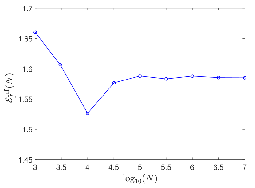
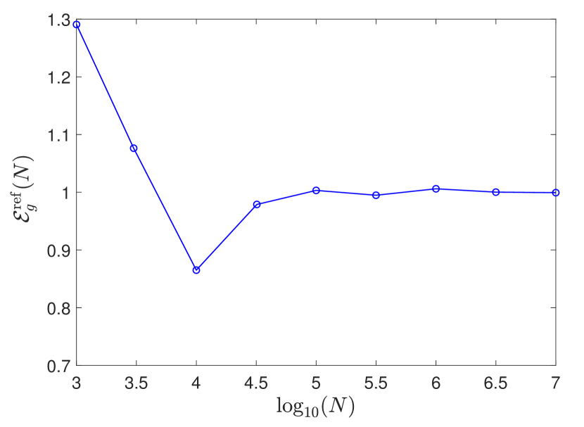
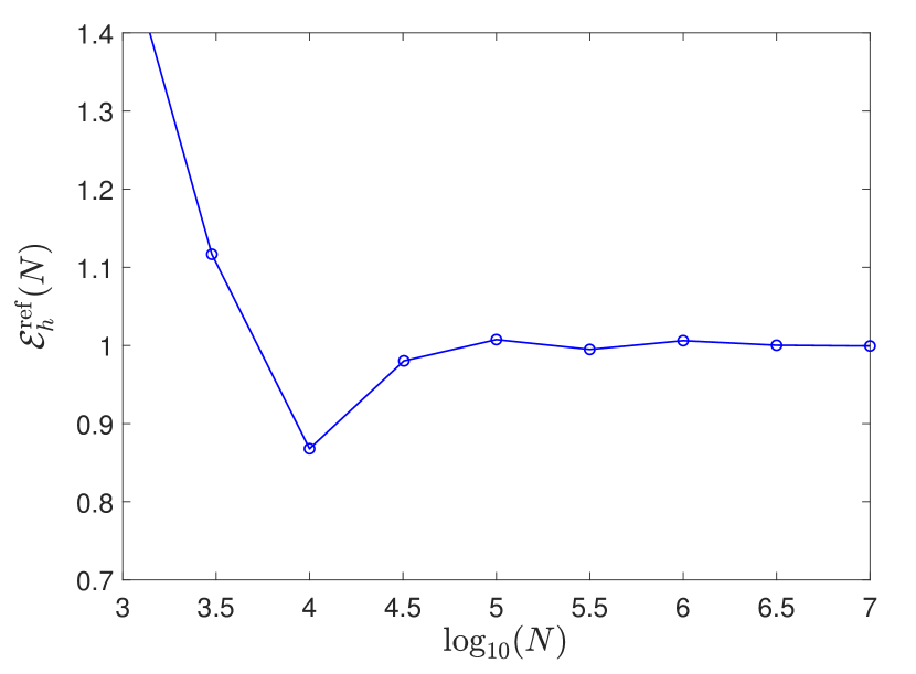
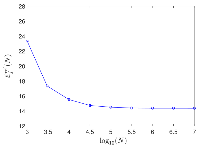
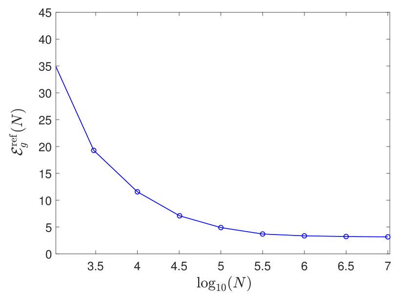
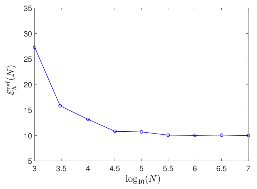
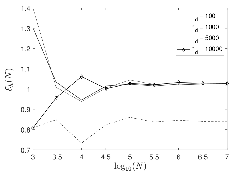
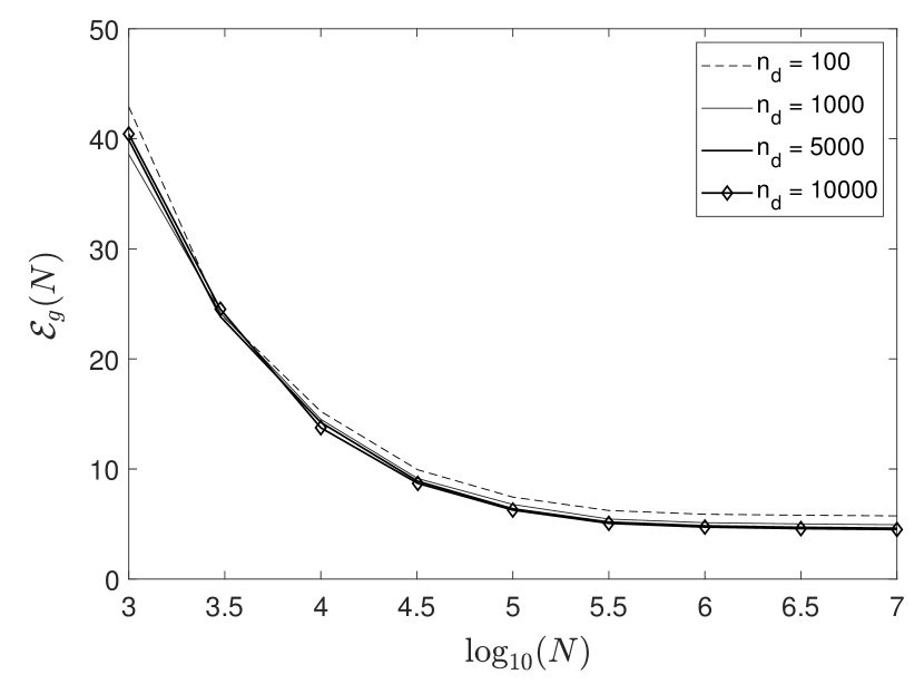
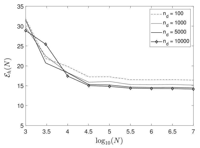
The convergence analysis with respect to is done for two values of . Fig. 1 concerns the results for , while Fig. 2 concerns the results for .
(i) Gaussian reference case. For the Gaussian reference case, for which the probability density function of is defined at the beginning of Section 5, the use of formulas defined by Eqs. (5.5) to (5.7) yields for and for .
For analyzing the convergence of the polynomial chaos expansions of this Gaussian reference case, the functions , and are computed using Eqs. (5.2), (5.3), and (5.4), respectively. The graphs of these functions are displayed in Figs. 1(a), 1(b), and 1(c) for , and in
Figs. 1(d), 1(e), and 1(f) for .
For , we have for and
for . These values are very close to the reference values that show a complete convergence and a full validation of the software code devoted to the computation of the polynomial-chaos-expansion coefficients based on the theory presented in Section 4.
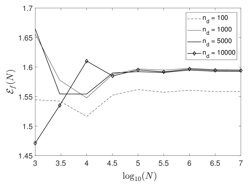
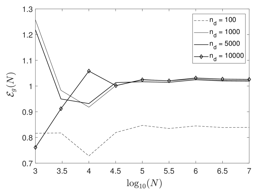
(ii) Gaussian case with GKDE representation. With respect to software code validation, this case does not provide anything more than the Gaussian reference case presented in (i), because the algorithms for calculating the coefficients of polynomial chaos expansions are independent of the choice of the probability density of . What this analysis shows for this Gaussian case is the influence of the number of points in the training dataset on the estimation of by the GKDE method (given by Eq. (2.3)), compared to the exact expression (which corresponds to as ). Therefore, for the Gaussian case with the GKDE estimation of defined by Eq. (2.3), we have considered four values of , which are , , , and . For the convergence analysis of the polynomial chaos expansions, the functions , and are computed using Eqs. (5.2), (5.3), and (5.4), respectively. The graphs of these functions are displayed in Figs. 2(a), 2(b), and 2(c) for , and in Figs. 2(d), 2(e), and 2(f) for . For , we have for and for . These values are close to the reference values for and slightly further away for . This does not call into question either the theoretical formulation proposed or the validation of the software code. This difference is simply due to the convergence of towards as a function of for a fixed value of . We know that the larger is, the larger must be. However, in the context of the probabilistic learning on manifolds approach, the eigenfunctions associated with the first eigenvalues of the Fokker-Planck operator that we are looking for are only used to construct a vector basis for the projection of the data, and replacing the exact operator with an approximate operator, constructed with a small training dataset, does not introduce any difficulties (see, for example, [1]).
6 Quantum computing formulation
The eigenproblem given in Eq. (3.17) is fully equivalent to a time-independent Schrödinger equation, where acts as the Hamiltonian and represents the corresponding eigenstate (or wavefunction). Solving this eigenproblem is commonly approached in the quantum mechanics community via projection (using the variational principle) onto a tensor-product basis spanning the full space [42, 43, 44, 45]. This approach is feasible only for low dimensionality , as its computational cost scales exponentially with . For large dimensional problems, alternative approximations using specific tensor decompositions are sometimes employed [46, 47, 48], though these schemes do not completely alleviate the exponential scaling. Recent advances in quantum computing offer potential for encoding the wavefunctions and their operations, even in high-dimensional problems (see for instance that quantum computers now have more than 1000 qubits [49]). This encoding becomes possible by mapping the system, as defined by the operator , onto a quantum computer, thereby representing wavefunctions and operations as qubits. While much of the research community is focused on electronic structure problems [50], new efforts are emerging to adapt other quantum problems for quantum computation [13, 14, 51]. For completeness, we depict here the general approach as follows: (i) choice of a basis, (ii) second quantization, and (iii) mapping onto qubits.
6.1 Choice of the basis
The first step is to adopt a finite basis representation (spectral method), for which we can easily rewrite Eq. (3.17) in a second quantized form. In our case, all dimensions are distinguishable, such that operators acting on different coordinates commute, and we must use different basis functions for each dimension. In line with section 3.7, we employ a basis of Hermite polynomials as a working basis. A common practice in the quantum mechanical community is to absorb the measure into the basis, where is defined in Definition 2. We also switch to the physicists’ convention for the Hermite polynomials during the process of building the basis. Furthermore, we perform an affine transformation on each coordinate, , to adapt the basis to improve convergence, where allows for a shift of the coordinate , if needed. For coordinate , the resulting basis is such that
for which the measure is and where is defined in Definition 2. These basis functions are the normalized eigenfunctions of the operator . By projecting Eq. (3.17) onto this basis, the eigenproblem becomes a matrix diagonalization, where the eigenstate is expanded as
| (6.1) |
where , , and , where are the maximum index that basis functions of the degree of freedom can have. Therefore, there are basis functions per degree of freedom, and the total number of one-dimensional basis functions, including all degrees of freedom, is . It should be noted that does not represent the number of basis functions in the tensor product space, which is not explicitly used in quantum computing. This concept lies at the heart of the advantage offered by quantum computing and is reminiscent of analog computing, but in the quantum realm.
6.2 Second quantization
On our way to express the eigenproblem on a quantum computer, we use the second quantization formalism [52, 53], which is particularly suited for encoding the qubits. In this formalism, all the basis functions can be generated from by employing the so-called creation operator
with such that with . By use of the creation operator, one can rewrite the solution in the so-called Fock space, where the basis functions are described by occupation numbers that we denote by
Similarly, we define the annihilation operator
with . Note that and are adjoint one to the other. Knowing the effect of and on the basis, we can rewrite all operators involved in Eq. (4.32) using the identities
Then, using the commutator , one can express and all monomials in the so-called normal ordering (with creation operators on the left of the annihilation operators) as follows,
| (6.2) | ||||
| (6.3) |
where is the double factorial, and returns the integer part of . For example, a quadratic term is given by . Note that Eq. (6.3) results from the expansion of the operator . The double sum and the double factorial reflect the combinatorics arising from the commutation relation . With these expressions at hand, the approximation of the Fokker-Planck operator , as defined by Eq. (3.19), can be expressed in a general form for a truncation at order with realizations of the Gaussian random variable ,
| (6.4) |
where the coefficients are obtained by substituting the expression from Eq. (6.3) into Eq. (4.32) and combining it with Eq. (6.2) into Eq. (3.19). Employing the form given in Eq. (6.4) is convenient, as the action of the creation and annihilation operators can easily be computed using the fact that
6.3 Map onto a system of qbits
Qubits are 2-level quantum systems, expressed as , that compose the quantum computers. To exploit quantum computing, we need to map the system of interest to the system of qubits. Rewriting the Fokker-Planck operator in a basis of qubits is not unique. Two mappings exist: the “direct” map [54], which we employ here due to its simplicity, and the “compact” map [55], which reduces the number of required qubits. An alternative approach involves using quantum computers based on bosonic modes (harmonic oscillators) instead of qubits, or hybrid architectures combining oscillators and qubits, where additional mappings and other quantum circuits construction stategies can also be explored [56, 57]. Here, we utilize the direct map [54, 13, 51]: the occupation of is represented by the occupation of a corresponding qubit state , such that a single qubit describes the occupation of a single basis function for a given degree of freedom, . In the direct map, the total number of qubit is given by , the total number of basis functions across all degrees of freedom as defined in Section 6.1. The qubit state corresponding to , associated with the degree of freedom , is rewritten, assuming that excatly one qubit is in the state at position , while all others are in the state :
| (6.5) |
By employing this notation, products of creation and annihilation operators on a basis function take the form
| (6.6) |
where is the imaginary number, . The operators and are Pauli matrices associated with the qubit used in the description of the degree of freedom . The hat indicates the matrix representation in the basis where individual qubits are represented as vectors and . Then, we can build the operator as
| (6.7) |
Equation (6.7) sums over all valid to form the full operator in qubit space, ensuring that each can transition to with the usual harmonic‐oscillator amplitude.
7 Quantum operations and measurements: quantum circuit
The construction of quantum states and the measurement of their observables are fundamental steps in the development of more advanced quantum algorithms. In this section, we provide an overview of these foundational concepts, particularly for readers who may be less familiar with quantum computing.
Manipulating qubits is achieved through quantum operations that are unitary transformations. Hence, the eigensolution that we seek can be expressed as , where represents the vacuum state of qubits (i.e., all qubits initialized in their ground state). Because individual qubits are 2-level systems, we can employ single-qubit transformations from , such as , , and , where , , and are the Pauli matrices (noting that ). Transformations acting on pairs, triplets, or more qubits can be built as tensor products of unitaries from , and more complex multi-qubit transformations generally involve entanglement and interactions between qubits. For example, the Pauli group (composed of tensor products of Pauli operators and the identity) forms a complete basis for constructing any multi-qubit unitary transformation [58]. In view of Eq. (6.5), constructing a specific state is equivalent to creating a superposition of collective qubit states by applying suitable unitary transformations to single qubits, pairs of qubits, or larger subsets of qubits. Such transformations are implemented on quantum computers via quantum gates, which are the fundamental building blocks of quantum circuits. Examples of commonly used quantum gates [59, 60] include the Hadamard gate , the phase gate , and the Controlled-NOT gate for two qubits, such that
where is the identity and is the Pauli-x matrix. To construct eigenstates, one needs a set of universal quantum gates that can reconstruct any unitary transformation in the qubit Hilbert space can be approximated to arbitrary precision [59, 58]. By successively applying these gates, one can construct quantum circuits that generate specific quantum states.
The target solutions of the FKP equation span only a subset of the qubits’ Hilbert space. This subset is restricted because certain qubit states are not valid representations of the basis states defined in Section 6.1. For instance, qubit states of the form do not correspond to any valid basis state. This is due to the constraint that, for each degree of freedom , only one qubit can take the value among the qubits assigned to describe . Mathematically, this constraint is expressed as
To address this issue, two possible strategies can be employed: i) adding constraints to the optimization process to explicitly enforce the condition for all , or ii) restricting the set of unitary transformations so that they inherently respect the constraint. This can be achieved by constructing transformations exclusively from the creation and annihilation operators, ensuring that and are always employed in pairs of the form .
Extracting information from quantum states is accomplished through quantum measurements of physical observables of interest. This measurement process is inherently probabilistic and results in the irreversible collapse of the quantum state. For example, assuming that an observable has an eigendecomposition , where is the number of qubits, measuring on a quantum state returns an eigenvalue with probability . After the measurement, the quantum state collapses to the corresponding eigenstate . As a result, many measurements (realizations) are required to statistically estimate the expectation value . For example, in quantum chemical applications using the Variational Quantum Eigensolver (VQE) framework, the number of measurements typically required is on the order of [61]. Only observables that are diagonal in the computational (qubit) basis can be directly measured, i.e., observables built as tensor products of and for each qubit. Hence, it is necessary to decompose the observable as , where each fragment can be efficiently transformed into a diagonal form via a suitable unitary transformation . This decomposition implies that the state of interest must also be transformed according to the same unitary operation before measuring each fragment. Reconstructing the expectation value requires combining all measurement outcomes on a classical computer (see, for instance, [62, 63, 64] for efficient measurement strategies). An alternative approach to measurement involves using the Hadamard test [58], which will be discussed in Section 8.2 and serves as an example of a measurement technique.
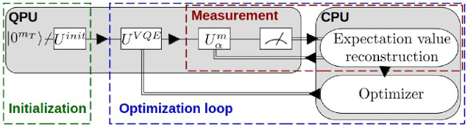
Considering the two key steps—construction and measurement of a quantum state—a quantum processing unit operates in two corresponding phases: (i) construction and (ii) measurement, as illustrated in Fig. 3. The measurement process must be repeated a sufficient number of times to ensure convergence to the expectation value for a given fragment. Since each measurement irreversibly collapses the quantum state, the entire process, including the state construction, must be repeated for every realization. Then, a classical computer combines the results from all fragments to reconstruct the total expectation value .
8 Proposal for eigenstates construction and overlap extraction
As explained in Section 3.8, we have to compute , for all and for all , that is to say, using Eq. (3.31), to compute . This is achieved by first generating eigenstates as solution of Eq. (3.24), and second by calculating the following overlap .
8.1 Eigenstates construction
Some of the most extensively studied algorithms for solving eigenproblems are the Variational Quantum Eigensolver (VQE) [65, 61] and the Quantum Phase Estimation (QPE) [66, 58].
(i) QPE algorithm. The QPE algorithm typically involves the following steps:
1) Preparing an initial quantum state with a significant overlap with the target eigenstates.
2) Decomposing the propagator into a sequence of quantum gates for various times .
3) Computing and storing the overlaps between the resulting states and the initial state, also referred to as the autocorrelation function, for the chosen time intervals.
4) Performing a Fourier transform on the autocorrelation function to extract the eigenspectrum and measuring the resulting state to identify eigenstates with significant overlap with the initial state.
(ii) Rationale for presenting the QPE or VQE algorithm. One objective of this section is to illustrate for readers who are not specialists in scientific quantum computing how the essential coupling between a quantum computer and a classical computer operates. Given the complexity and non-trivial nature of the QPE algorithm, we choose to focus on the VQE approach, which can be introduced using simpler concepts. Furthermore, QPE requires substantially longer quantum circuits than VQE [67, 61], making the latter more practical for quantum computers in the Noisy Intermediate-Scale Quantum (NISQ) era, where quantum hardware remains limited [68]. We therefore focus on the VQE approach and provide here a brief overview.
(iii) VQE algorithm. The VQE approach is a hybrid quantum-classical algorithm [69] designed to approximate the lowest, “ground state”, eigensolutions of an eigenequation (see Fig. 4). It is based on the Rayleigh-Ritz variational principle, which states that any normalized trial wavefunction satisfies the inequality , where
is the Rayleigh quotient of the symmetric and positive operator (see Sections 3.5 and 3.6).
Equality occurs when is the ground-state wavefunction.
Algorithm VQE combines the capabilities of quantum and classical computers to iteratively refine a parameterized trial wavefunction in order to minimize .
The quantum computer is used to construct the trial wavefunction and estimate the Rayleigh quotient, while the classical computer optimizes the parameters of the wavefunction.
(iii-1) Initial guess, assumed to be a good approximation to the exact solution.
The first step in VQE is to define an initial guess , which serves as an approximation to the exact eigenstate.
A good initial guess reduces the number of iterations required for convergence.
The construction of is performed on a classical computer, using a mean-field approximation (e.g., a single Hartree product solution), or by solving a zeroth-order Hamiltonian [70, 53].
The initial guess is then encoded on the quantum computer using a unitary transformation , such that .
(iii-2) Parameterization of the trial wavefunction. The second step is parameterizing the trial wavefunction using a unitary ansatz , where are the parameters to be optimized.
Ideally, the ansatz would explore the entire Hilbert space, for example employing operations from the Pauli group.
However, the exponential scaling of the number of elements with the number of qubits makes this computationally infeasible, as the optimization is performed on a classical computer.
Instead, a structured, parameterized ansatz, named the VQE ansatz, is employed.
Common choices include Unitary Coupled Cluster [65], Hardware-Efficient Ansatz [71], and Quantum Coupled Cluster [72].
The ansatz is typically expressed as a product of parameterized unitary operations, , and the trial state is now expressed as
.
(iii-3) Optimization employing the classical computer. Once the ansatz is defined, the parameters are optimized to minimize the Rayleigh quotient , which corresponds to the expectation value of .
The optimization process is carried out on a classical computer using gradient-free methods, such as the Nelder-Mead simplex algorithm [73], or gradient-based methods like gradient descent. Gradients can be computed either analytically or through finite-difference approximations (see, for instance, [74, 75, 76]).
These methods require additional quantum measurements to compute extra points or derivatives, which increases the computational overhead.
(iii-4) Computing other eigenstates. Generating other eigenstates with , the “excited states”, is possible within the VQE framework. Assuming that has already been obtained, the algorithm can be modified to target excited states by either adding a penalty or imposing a constraint on the symmetry of the excited state, when applicable [77], or by enforcing the orthogonality requirement [78].
8.2 Overlap extraction
Assuming that eigenstates are obtained, it becomes possible to extract overlaps of the form . To achieve this, we first express the overlap as , where . Note that is the tensor-product basis; consequently, this expression cannot be computed directly. This is why we rewrite it as a manageable single product. Then, the objectives are twofold: i) construct and on the quantum computer, and ii) extract the overlap as a measurement process.
The construction of depicted in Sec. 8.1. Regarding the construction of , we rewrite this state as a direct product:
| (8.1) |
where and are written as
| (8.2) |
Note that substituting Eq. (8.2) into (8.1) effectively yields . Each factor in the product on the right-hand-side of Eq. (8.1) is constructed on the quantum computer by using a product of unitaries. We give here a simple algorithm for their constructions. Starting with all qubits associated with in their ground state, the vacuum state, we apply successive rotations to distribute the coefficients on the qubit states that encode . These rotations are defined by
| (8.3) |
As expected, the first rotation applied on the vacuum gives a superposition of two terms: , the second term being the one of interest. If we apply the second rotation on this last obtained superposition, it would destroy . Instead, we must apply the second rotation only on the term containing . This is achieved by using an “anti-controlled” rotation,
which applies the rotation only if . Indeed, with the controlled rotation, we now obtain
| (8.4) |
To generalize this scheme, we need to define anti-controlled rotations of the form , where the anti-control test is applied on all preceeding qubits, . These anti-controlled rotations are then used in place of the rotations . The circuits that achieve this construction of a factor is depicted in Fig. 5.
Equipped with this circuit, the unitary transformation,, that builds is given by
To extract the overlap , we propose using the Hadamard test [58]. In combination with the qubits used to construct , the Hadamard test employs an additional “ancilla” qubit. Using the Hadamard gate and controlled-unitaries, this ancilla qubit is used to construct a superposition of and in the entangled form (see Fig. 6),
By measuring for the ancilla qubit, the result will be with probability , or with probability , and where denotes the real part. After reconstructing the probabilities , the overlap is extracted as (accounting for the fact that ).
9 Conclusions
In this paper, we have developed a methodology and demonstrated a quantum computing framework to address a key challenge in probabilistic learning on manifolds (PLoM). This challenge involves solving the spectral problem of the high-dimensional FKP operator, a task that classical computational methods cannot efficiently handle. Notably, this problem may also be relevant to frameworks and applications beyond those that motivated the developments presented in this work.
In addition to the methodological aspects, we introduced a polynomial chaos expansion in the Gaussian Sobolev space for the potential in the Schrödinger operator associated with the FKP operator. This approach preserves the algebraic properties of the potential and enables second quantization through the introduction of creation and annihilation operators. By reformulating the eigenvalue problem in Fock space, we derived explicit formulas for both the Laplacian and the potential, facilitating the implementation of the FKP operator as a Hamiltonian in quantum circuits.
To provide a comprehensive perspective, we also included a brief overview of foundational concepts related to the construction of quantum states and the measurement of their observables, particularly for readers less familiar with quantum computing. To illustrate the essential coupling between a quantum computer and a classical computer, we chose to present the Variational Quantum Eigensolver (VQE) approach instead of the Quantum Phase Estimation (QPE) algorithm, given the latter’s greater complexity and non-trivial nature. Furthermore, QPE requires longer quantum circuits, with a larger the number of qubits than what is currently available in the NISQ era [49] and the ability for error correction [67, 79].
The next step in this work will be the implementation of the proposed method on a quantum computer.
Conflict of interest
The author declares that he has no conflict of interest.
References
- [1] C. Soize, R. Ghanem, Transient anisotropic kernel for probabilistic learning on manifolds, Computer Methods in Applied Mechanics and Engineering 432 (2024) 117453. doi:10.1016/j.cma.2024.117453.
- [2] B. Liu, M. Ortiz, F. Cirak, Towards quantum computational mechanics, Computer Methods in Applied Mechanics and Engineering 432 (2024) 117403. doi:10.1016/j.cma.2024.117403.
- [3] A. Wulff, B. Chen, M. Steinberg, Y. Tang, M. Möller, S. Feld, Quantum computing and tensor networks for laminate design: a novel approach to stacking sequence retrieval, Computer Methods in Applied Mechanics and Engineering 432 (2024) 117380. doi:10.1016/j.cma.2024.117380.
- [4] Y. Xu, J. Yang, Z. Kuang, Q. Huang, W. Huang, H. Hu, Quantum computing enhanced distance-minimizing data-driven computational mechanics, Computer Methods in Applied Mechanics and Engineering 419 (2024) 116675. doi:10.1016/j.cma.2023.116675.
- [5] H. Ma, M. Govoni, G. Galli, Quantum simulations of materials on near-term quantum computers, npj Computational Materials 6 (1) (2020) 85. doi:10.1038/s41524-020-00353-z.
- [6] C. Micheletti, P. Hauke, P. Faccioli, Polymer physics by quantum computing, Physical Review Letters 127 (8) (2021) 080501. doi:10.1103/PhysRevLett.127.080501.
- [7] K. Mizuta, M. Fujii, S. Fujii, K. Ichikawa, Y. Imamura, Y. Okuno, Y. O. Nakagawa, Deep variational quantum eigensolver for excited states and its application to quantum chemistry calculation of periodic materials, Physical Review Research 3 (4) (2021) 043121. doi:10.1103/PhysRevResearch.3.043121.
- [8] O. M. Raisuddin, S. De, Feqa: Finite element computations on quantum annealers, Computer Methods in Applied Mechanics and Engineering 395 (2022) 115014. doi:10.1016/j.cma.2022.115014.
- [9] Y. Wang, J. E. Kim, K. Suresh, Opportunities and challenges of quantum computing for engineering optimization, Journal of Computing and Information Science in Engineering 23 (6) (2023) 060817. doi:10.1115/1.4062969.
- [10] Z. Ye, X. Qian, W. Pan, Quantum topology optimization via quantum annealing, IEEE Transactions on Quantum Engineering 4 (2023) 1–15. doi:10.1109/TQE.2023.3266410.
- [11] H. Risken, The Fokker-Planck Equation, Second Edition, Springer Verlag, Berlin, Heidelberg, 1989.
- [12] C. W. Gardiner, Handbook of Stochastic Methods, Second Edition, Springer Verlag, Berlin, Heidelberg, 1985.
- [13] S. McArdle, A. Mayorov, X. Shan, S. Benjamin, X. Yuan, Digital quantum simulation of molecular vibrations, Chem. Sci. 10 (22) (2019) 5725–5735. doi:10.1039/C9SC01313J.
- [14] N. P. D. Sawaya, J. Huh, Quantum Algorithm for Calculating Molecular Vibronic Spectra, J. Phys. Chem. Lett. 10 (13) (2019) 3586–3591. doi:10.1021/acs.jpclett.9b01117.
- [15] Ó. Amaro, L. I. I. Gamiz, M. Vranic, Variational Quantum Simulation of the Fokker-Planck Equation applied to Quantum Radiation Reaction, arXiv (Nov. 2024). arXiv:2411.17517, doi:10.48550/arXiv.2411.17517.
- [16] P. Malliavin, Gaussian Sobolev spaces and stochastic calculus of variations, in: Integration and Probability, Vol. 157 of Graduate Texts in Mathematics, Springer, New York, NY, 1995, pp. 229–252. doi:10.1007/978-1-4612-4202-4_5.
- [17] C. Soize, R. Ghanem, Data-driven probability concentration and sampling on manifold, Journal of Computational Physics 321 (2016) 242–258. doi:10.1016/j.jcp.2016.05.044.
- [18] C. Soize, R. Ghanem, Probabilistic learning on manifolds, Foundations of Data Science 2 (3) (2020) 279–307. doi:10.3934/fods.2020013.
- [19] C. Soize, R. Ghanem, Physics-constrained non-Gaussian probabilistic learning on manifolds, International Journal for Numerical Methods in Engineering 121 (1) (2020) 110–145. doi:10.1002/nme.6202.
- [20] C. Soize, R. Ghanem, Probabilistic learning on manifolds constrained by nonlinear partial differential equations for small datasets, Computer Methods in Applied Mechanics and Engineering 380 (2021) 113777. doi:10.1016/j.cma.2021.113777.
- [21] C. Soize, Probabilistic learning inference of boundary value problem with uncertainties based on Kullback-Leibler divergence under implicit constraints, Computer Methods in Applied Mechanics and Engineering 395 (2022) 115078. doi:10.1016/j.cma.2022.115078.
- [22] C. Soize, R. Ghanem, Probabilistic-learning-based stochastic surrogate model from small incomplete datasets for nonlinear dynamical systems, Computer Methods in Applied Mechanics and Engineering 418 (2024) 116498. doi:10.1016/j.cma.2023.116498.
- [23] C. Soize, R. Ghanem, Probabilistic learning on manifolds (PLoM) with partition, International Journal for Numerical Methods in Engineering 123 (1) (2022) 268–290. doi:10.1002/nme.6856.
- [24] C. Soize, Probabilistic learning constrained by realizations using a weak formulation of fourier transform of probability measures, Computational Statistics 38 (4) (2023) 1879–1925. doi:10.1007/s00180-022-01300-w.
- [25] R. Coifman, S. Lafon, A. Lee, M. Maggioni, B. Nadler, F. Warner, S. Zucker, Geometric diffusions as a tool for harmonic analysis and structure definition of data: Diffusion maps, PNAS 102 (21) (2005) 7426–7431. doi:10.1073/pnas.0500334102.
- [26] R. Coifman, S. Lafon, Diffusion maps, Applied and Computational Harmonic Analysis 21 (1) (2006) 5–30. doi:10.1016/j.acha.2006.04.006.
- [27] C. Soize, Polynomial chaos expansion of a multimodal random vector, SIAM-ASA Journal on Uncertainty Quantification 3 (1) (2015) 34–60. doi:10.1137/140968495.
- [28] A. Bowman, A. Azzalini, Applied Smoothing Techniques for Data Analysis: The Kernel Approach With S-Plus Illustrations, Vol. 18, Oxford University Press, Oxford: Clarendon Press, New York, 1997. doi:10.1007/s001800000033.
- [29] T. Duong, A. Cowling, I. Koch, M. Wand, Feature significance for multivariate kernel density estimation, Computational Statistics & Data Analysis 52 (9) (2008) 4225–4242. doi:10.1016/j.csda.2008.02.035.
- [30] J. E. Gentle, Computational statistics, Springer, New York, 2009. doi:10.1007/978-0-387-98144-4.
- [31] G. Givens, J. Hoeting, Computational Statistics, 2nd Edition, John Wiley and Sons, Hoboken, New Jersey, 2013.
- [32] J. L. Doob, Stochastic processes, John Wiley & Sons, New York, 1953.
- [33] I. I. Guikhman, A. Skorokhod, Introduction à la Théorie des Processus Aléatoires, Edition Mir, 1980.
- [34] A. Friedman, Stochastic Differential Equations and Applications, Dover Publications, Inc., Mineola, New York, 2006.
- [35] C. Soize, The Fokker-Planck Equation for Stochastic Dynamical Systems and its Explicit Steady State Solutions, Vol. Series on Advances in Mathematics for Applied Sciences: Vol 17, World Scientific, Singapore, 1994. doi:10.1142/2347.
- [36] C. Soize, R. Ghanem, C. Safta, X. Huan, Z. P. Vane, J. C. Oefelein, G. Lacaze, H. N. Najm, Q. Tang, X. Chen, Entropy-based closure for probabilistic learning on manifolds, Journal of Computational Physics 388 (2019) 528–533. doi:10.1016/j.jcp.2018.12.029.
- [37] N. Wiener, The homogeneous chaos, American Journal of Mathematics 60 (1) (1938) 897–936.
- [38] R. H. Cameron, W. T. Martin, The orthogonal development of non-linear functionals in series of Fourier-Hermite functionals, Annals of Mathematics 48 (2) (1947) 385–392. doi:10.2307/1969178.
- [39] P. Krée, C. Soize, Mathematics of Random Phenomena, Reidel Pub. Co, 1986, (first published by Bordas in 1983 and also published by Springer Science & Business Media in 2012).
- [40] R. J. Serfling, Approximation theorems of mathematical statistics, Vol. 162, John Wiley & Sons, 1980.
- [41] C. Soize, Uncertainty Quantification. An Accelerated Course with Advanced Applications in Computational Engineering, Springer, New York, 2017. doi:10.1007/978-3-319-54339-0.
-
[42]
D. Gottlieb, S. A. Orszag,
Numerical
Analysis of Spectral Methods, Society for Industrial and Applied
Mathematics, 1977.
arXiv:https://epubs.siam.org/doi/pdf/10.1137/1.9781611970425, doi:10.1137/1.9781611970425.
URL https://epubs.siam.org/doi/abs/10.1137/1.9781611970425 - [43] J. C. Light, T. Carrington, Discrete-Variable Representations and their Utilization, in: Advances in Chemical Physics, John Wiley & Sons, Inc., Hoboken, NJ, USA, 2000, pp. 263–310. doi:10.1002/9780470141731.ch4.
-
[44]
D. J. Tannor,
Introduction
to Quantum Mechanics: A Time-Dependent Perspective, Harvard, 2007.
URL https://ui.adsabs.harvard.edu/abs/2007iqm..book.....T/abstract - [45] F. Gatti, B. Lasorne, H.-D. Meyer, A. Nauts, Applications of quantum dynamics in chemistry, Vol. 98, Springer, 2017.
- [46] H.-D. Meyer, F. Gatti, G. A. Worth, Multidimensional quantum dynamics: MCTDH theory and applications, John Wiley & Sons, 2009.
- [47] U. Schollwöck, The density-matrix renormalization group in the age of matrix product states, Ann. Phys. 326 (1) (2011) 96–192. doi:10.1016/j.aop.2010.09.012.
- [48] M. Bachmayr, Low-rank tensor methods for partial differential equations, Acta Numer. 32 (2023) 1–121.
- [49] D. Castelvecchi, Ibm releases first-ever 1,000-qubit quantum chip, Nature 624 (2023) 238. doi:10.1038/d41586-023-03854-1.
- [50] B. Fauseweh, Quantum many-body simulations on digital quantum computers: State-of-the-art and future challenges, Nat. Commun. 15 (2123) (2024) 1–13. doi:10.1038/s41467-024-46402-9.
- [51] Y. Wang, L. M. Sager-Smith, D. A. Mazziotti, Quantum simulation of bosons with the contracted quantum eigensolver, New J. Phys. 25 (10) (2023) 103005. doi:10.1088/1367-2630/acf9c3.
- [52] P. R. Surján, Second Quantized Approach to Quantum Chemistry, Springer, Berlin, Germany, 1989.
- [53] J. M. Bowman, Vibrational Dynamics of Molecules, World Scientific Publishing Company, Singapore, 2021. doi:10.1142/12305.
- [54] R. Somma, G. Ortiz, J. E. Gubernatis, E. Knill, R. Laflamme, Simulating physical phenomena by quantum networks, Phys. Rev. A 65 (4) (2002) 042323. doi:10.1103/PhysRevA.65.042323.
- [55] L. Veis, J. Višňák, H. Nishizawa, H. Nakai, J. Pittner, Quantum chemistry beyond Born–Oppenheimer approximation on a quantum computer: A simulated phase estimation study, Int. J. Quantum Chem. 116 (18) (2016) 1328–1336. doi:10.1002/qua.25176.
- [56] E. Crane, K. C. Smith, T. Tomesh, A. Eickbusch, J. M. Martyn, S. Kühn, L. Funcke, M. A. DeMarco, I. L. Chuang, N. Wiebe, A. Schuckert, S. M. Girvin, Hybrid Oscillator-Qubit Quantum Processors: Simulating Fermions, Bosons, and Gauge Fields, arXiv (Sep. 2024). arXiv:2409.03747, doi:10.48550/arXiv.2409.03747.
- [57] S. Malpathak, S. D. Kallullathil, A. F. Izmaylov, Simulating Vibrational Dynamics on Bosonic Quantum Devices, arXiv (Nov. 2024). arXiv:2411.17950, doi:10.48550/arXiv.2411.17950.
- [58] M. A. Nielsen, I. L. Chuang, Quantum computation and quantum information, Cambridge university press, 2010.
- [59] A. Barenco, C. H. Bennett, R. Cleve, D. P. DiVincenzo, N. Margolus, P. Shor, T. Sleator, J. A. Smolin, H. Weinfurter, Elementary gates for quantum computation, Phys. Rev. A 52 (5) (1995) 3457–3467. doi:10.1103/PhysRevA.52.3457.
- [60] I. Djordjevic, Chapter 3 - Quantum Circuits and Quantum Information Processing Fundamentals, in: Quantum Information Processing and Quantum Error Correction, Academic Press, Cambridge, MA, USA, 2012, pp. 91–117. doi:10.1016/B978-0-12-385491-9.00003-4.
- [61] J. Tilly, H. Chen, S. Cao, D. Picozzi, K. Setia, Y. Li, E. Grant, L. Wossnig, I. Rungger, G. H. Booth, J. Tennyson, The Variational Quantum Eigensolver: A review of methods and best practices, Phys. Rep. 986 (2022) 1–128. doi:10.1016/j.physrep.2022.08.003.
- [62] V. Verteletskyi, T.-C. Yen, A. F. Izmaylov, Measurement optimization in the variational quantum eigensolver using a minimum clique cover, The Journal of chemical physics 152 (12) (2020). doi:10.1063/1.5141458.
- [63] T.-C. Yen, A. F. Izmaylov, Cartan Subalgebra Approach to Efficient Measurements of Quantum Observables, PRX Quantum 2 (4) (2021) 040320. doi:10.1103/PRXQuantum.2.040320.
- [64] T.-C. Yen, A. Ganeshram, A. F. Izmaylov, Deterministic improvements of quantum measurements with grouping of compatible operators, non-local transformations, and covariance estimates, npj Quantum Inf. 9 (14) (2023) 1–7. doi:10.1038/s41534-023-00683-y.
- [65] A. Peruzzo, J. McClean, P. Shadbolt, M.-H. Yung, X.-Q. Zhou, P. J. Love, A. Aspuru-Guzik, J. L. O’Brien, A variational eigenvalue solver on a photonic quantum processor, Nature Communications 5 (1) (2014) 4213. doi:10.1038/ncomms5213.
- [66] A. Yu. Kitaev, Quantum measurements and the Abelian Stabilizer Problem, arXiv (Nov. 1995). arXiv:quant-ph/9511026, doi:10.48550/arXiv.quant-ph/9511026.
- [67] M. Reiher, N. Wiebe, K. M. Svore, D. Wecker, M. Troyer, Elucidating reaction mechanisms on quantum computers, Proc. Natl. Acad. Sci. U.S.A. 114 (29) (2017) 7555–7560. doi:10.1073/pnas.1619152114.
- [68] J. Preskill, Quantum Computing in the NISQ era and beyond, Quantum 2 (2018) 79. arXiv:1801.00862v3, doi:10.22331/q-2018-08-06-79.
- [69] J. R. McClean, J. Romero, R. Babbush, A. Aspuru-Guzik, The theory of variational hybrid quantum-classical algorithms, New Journal of Physics 18 (2) (2016) 023023. doi:10.1088/1367-2630/18/2/023023.
-
[70]
E. B. Wilson, Jr., J. C. Decius, P. C. Cross,
Molecular
Vibrations: The Theory of Infrared and Raman Vibrational Spectra (Dover Books
on Chemistry), Dover Publications, Mineola, NY, USA, 1980.
URL https://www.amazon.com/Molecular-Vibrations-Infrared-Vibrational-Chemistry/dp/048663941X - [71] A. Kandala, A. Mezzacapo, K. Temme, M. Takita, M. Brink, J. M. Chow, J. M. Gambetta, Hardware-efficient variational quantum eigensolver for small molecules and quantum magnets, Nature 549 (2017) 242–246. doi:10.1038/nature23879.
- [72] I. G. Ryabinkin, T.-C. Yen, S. N. Genin, A. F. Izmaylov, Qubit coupled cluster method: a systematic approach to quantum chemistry on a quantum computer, Journal of chemical theory and computation 14 (12) (2018) 6317–6326. doi:10.1021/acs.jctc.8b00932.
- [73] I. Miháliková, M. Friák, M. Pivoluska, M. Plesch, M. Saip, M. Šob, Best-Practice Aspects of Quantum-Computer Calculations: A Case Study of the Hydrogen Molecule, Molecules 27 (3) (2022) 597. doi:10.3390/molecules27030597.
- [74] J. Romero, R. Babbush, J. R. McClean, C. Hempel, P. J. Love, A. Aspuru-Guzik, Strategies for quantum computing molecular energies using the unitary coupled cluster ansatz, Quantum Sci. Technol. 4 (1) (2018) 014008. doi:10.1088/2058-9565/aad3e4.
- [75] L. Wang, J. Zhu, J. C. Spall, Mixed simultaneous perturbation stochastic approximation for gradient-free optimization with noisy measurements, in: 2018 Annual American Control Conference (ACC), IEEE, 2018, pp. 27–29. doi:10.23919/ACC.2018.8430974.
- [76] X. Bonet-Monroig, H. Wang, D. Vermetten, B. Senjean, C. Moussa, T. Bäck, V. Dunjko, T. E. O’Brien, Performance comparison of optimization methods on variational quantum algorithms, Phys. Rev. A 107 (3) (2023) 032407. doi:10.1103/PhysRevA.107.032407.
- [77] I. G. Ryabinkin, S. N. Genin, A. F. Izmaylov, Constrained Variational Quantum Eigensolver: Quantum Computer Search Engine in the Fock Space, J. Chem. Theory Comput. 15 (1) (2019) 249–255. doi:10.1021/acs.jctc.8b00943.
- [78] O. Higgott, D. Wang, S. Brierley, Variational Quantum Computation of Excited States, Quantum 3 (2019) 156. arXiv:1805.08138v5, doi:10.22331/q-2019-07-01-156.
- [79] L. Postler, S. Heuen, I. Pogorelov, M. Rispler, T. Feldker, M. Meth, C. D. Marciniak, R. Stricker, M. Ringbauer, R. Blatt, P. Schindler, M. Müller, T. Monz, Demonstration of fault-tolerant universal quantum gate operations, Nature 605 (2022) 675–680. doi:10.1038/s41586-022-04721-1.