2025 \startpage1
Han Bao et al.
Han Bao
Addressing Positivity Violations in Continuous Interventions through Data-Adaptive Strategies
Abstract
[Abstract]Positivity violations pose a key challenge in the estimation of causal effects, particularly for continuous interventions. Current approaches for addressing this issue include the use of projection functions or modified treatment policies. While effective in many contexts, these methods can result in estimands that potentially do not align well with the original research question, thereby leading to compromises in interpretability. In this paper, we introduce a novel diagnostic tool—the non-overlap ratio—to detect positivity violations. To address these violations while maintaining interpretability, we propose a data-adaptive solution, specially a "most feasible" intervention strategy. Our strategy operates on a unit-specific basis. For a given intervention of interest, we first assess whether the intervention value is feasible for each unit. For units with sufficient support –conditional on confounders– , we adhere to the intervention of interest. However, for units lacking sufficient support –as identified through the assessment of the non-overlap ratio– we do not assign the actual intervention value of interest. Instead, we assign the closest feasible value within the support region. We propose an estimator using g-computation coupled with flexible conditional density estimation to estimate high- and low support regions to estimate this new estimand. Through simulations, we demonstrate that our method effectively reduces bias across various scenarios by addressing positivity violations. Moreover, when positivity violations are absent, the method successfully recovers the standard estimand. We further validate its practical utility using real-world data from the CHAPAS-3 trial, which enrolled HIV-positive children in Zambia and Uganda.
keywords:
data-adaptive interventions; causal inference; positivity violations; HIV treatment1 Introduction
Causal inference methods have been extensively studied for binary treatments, where individuals are either exposed to a treatment or assigned to a control condition 1, 2. In this framework, the positivity assumption—requiring that each individual has a non-zero probability of receiving any treatment level under consideration within confounder strata—is crucial for the identifiability and unbiased estimation of causal effects.
Violations of the positivity assumption can be categorized as structural or practical 3, 4, 5. Structural violations occur when an intervention is inherently impossible, whereas practical violations arise when certain treatment levels are theoretically possible but are not observed in the data. Both types lead to non-overlap in the confounder space, where certain confounder patterns have a zero probability, either theoretical or estimated, of receiving specific treatment levels. These violations hinder the estimation of causal effects, making it challenging to draw reliable inferences.
In pharmacoepidemiological and public health studies, researchers often extend their focus to continuous interventions, where the treatment variable can take on a range of values. In this context, the estimation of the causal dose-response curve (CDRC)—which describes the relationship between the continuous treatment and the outcome—has gained increasing attention in the causal inference literature. The CDRC provides a nuanced understanding of causal effects of continuous interventions. However, estimating the CDRC introduces new challenges, particularly because the positivity assumption becomes more stringent with continuous interventions.
For continuous interventions, the positivity assumption is commonly violated due to the infinite dimensionality of the treatment space. This makes it virtually impossible to observe all potential treatment levels across all confounder combinations. The resulting sparsity in certain regions of the intervention space can lead to unstable or biased estimates, a challenge frequently overlooked in existing studies.
While methods adapted from binary treatments can be applied, they have limitations. Trimming, for example, excludes regions of the confounder space with poor overlap 6, removing individuals with extreme probabilities of treatment given their confounders. However, this approach may result in the loss of valuable data.
To tackle these challenges, researchers have developed specialized methods, including projection functions and g-computation-type plug-in estimators, which aim to mitigate the violation of the positivity assumption 4. One such approach is the weighted CDRC, which reweights and redefines the estimand of interest based on functions of the conditional support for the respective interventions 7. Additionally, machine learning techniques have proven effective in enhancing estimation accuracy by minimizing the risk of bias caused by model misspecification 8.
Another notable strategy involves modified treatment policies (MTPs) 9, 10, which redefine the intervention of interest based on the natural intervention (i.e., the level of treatment actually received). While MTPs can sometimes, if designed cleverly, substantially reduce the reliance on the positivity assumption, they (typically) alter the original research question, which may not be ideal in many cases (including the data example discussed in Section 5).
In this paper, we aim to improve both interpretability and applicability in addressing positivity violations for continuous interventions. Our contributions are:
-
1.
Defining and diagnosing positivity violations in practice: we introduce a practical framework for diagnosing positivity violations in continuous interventions. Specifically, we define the support using the high-density region of the conditional intervention distribution and propose a diagnostic metric, the non-overlap ratio, to quantify the severity of positivity violations.
-
2.
Introducing novel estimands to address positivity violations: we propose a framework of data-adaptive interventions—specifically, the most feasible intervention—to construct a new estimand that replaces unfeasible interventions with the closest feasible values based on the observed data. This approach improves both interpretability and applicability, allowing researchers to approximate the standard CDRC without significantly deviating from the original intervention strategy.
By addressing the challenges posed by positivity violations in continuous interventions, our proposed methods provide a practical and reliable framework for causal inference. We demonstrate the effectiveness of our approach through simulations and real data analysis, highlighting the advantages of our method in mitigating positivity violations while preserving interpretability through minimal adjustments to the infeasible interventions.
2 From Identification Assumptions to Positivity Violations
2.1 Notation
Consider cross-sectional data at a single time point. In this setup:
-
•
is the outcome, with representing the outcome space.
-
•
stands for the intervention, with being the intervention space.
-
•
represents a set of confounders, where . The space of all such confounders is given by .
We use uppercase letters to denote random variables and lowercase letters for their particular realizations. The temporal order of these variables ranges from to , followed by and . Central to our analysis is the concept of counterfactual outcomes. For any subject , the counterfactual outcome denotes the potential outcome had the intervention been set to a specific level in the intervention space .
Given a probability space defined by , where is the product space , the observed data structure can be expressed as:
Here, is distributed according to , and the observations are independent and identically distributed.
For a sample of observations from the distribution , the dataset is given by .
Further notation:
-
•
The marginal probability distribution of treatment is represented by , and its probability density function is .
-
•
For confounders , their marginal probability distribution and density functions are and , respectively.
-
•
The conditional probability distribution of the treatment given the confounders is , and its density function is .
2.2 Consequences of Positivity Violations
In causal inference, assumptions like consistency, exchangeability, and positivity are critical for identifying causal effects. Among these, positivity, often considered as a well-understood assumption, plays a unique role in ensuring that causal treatment effects can be properly identified.
The widely accepted positivity assumption, often referred to as the strong positivity assumption, states that each possible treatment level must have a positive probability of occurring within every stratum of the confounders 4:
| (1) |
The positivity assumption requires a non-zero infimum of density in the entire intervention space , yet depending on the intervention distribution. While much attention has been focused on understanding positivity as an abstract assumption for identification, there is a gap in the literature when it comes to detecting positivity violations in real-world data. Moreover, even when the identification assumptions are met, regions with sparse data can significantly impact the extent of bias and precision at the estimation stage, see Appendix Addressing Positivity Violations in Continuous Interventions through Data-Adaptive Strategies for details. Reliable causal estimation becomes challenging due to inadequate representation across the entire intervention domain for all confounder patterns, which can introduce biases and limit the generalizability of the estimated causal effects.
2.3 Determination of Positivity Violations
Determining whether data sufficiently supports a given intervention requires assessing if the density of the data is so low that it becomes nearly impossible to observe it in finite sample settings. This leads to a crucial insight: introducing a threshold, , for the density function to identify potential positivity violations. Given a specific realization of confounders, , an intervention of interest can be classified as follows:
| (2) |
In the case of binary interventions, (near) positivity violations occur when the conditional probability of observing an intervention is extremely low or even zero. Given the discrete nature of the intervention, the concepts of density and probability coincide, making the detection of violations relatively straightforward. However, for continuous interventions, the situation is more complex. The density function must satisfy the property , meaning the range of is contingent on the span of the intervention space . This variability complicates the establishment of static thresholds; for instance, setting as "not supported" or as "sufficiently supported" may not be appropriate across different contexts.
Establishing a fixed threshold for continuous interventions thus presents significant challenges. Recognizing this, we propose a novel approach as a key contribution of this paper. This approach redefines and more accurately determines positivity violations in practical settings by utilizing a dynamic diagnostic measure.
2.3.1 Proposal 1: Definition of support and diagnostic using High-Density Region (HDR)
Conditional Support: high-density region
To address the issue of poorly supported intervention areas, we propose a method that dichotomizes the normalized -values. This approach involves identifying regions of the intervention space, , where the support is either strong or lacking, based on a probability threshold. Specifically, we partition into two parts, and its complement , according to a specified threshold depending on . Given the threshold for detection of non-overlap, named the coverage level, , the region is defined such that the probability measure satisfies . An intervention can then be categorized as follows:
| (3) |
Defining as the high-density region—essentially the practical support—is a relatively straightforward process. This is accomplished by leveraging the concept of high-density regions, proposed by Hyndman 11. Specifically, the high-density region for a continuous intervention is defined by:
| (4) |
where is the adaptive threshold constant, determined such that the condition is satisfied.
An illustrative example of this concept is provided in Figure 1, where the green regions represent the conditional support, indicating where a intervention is well-supported by the data. In contrast, the grey regions highlight areas with positivity violations, where a intervention is poorly supported. The total probability of the green region sums to the coverage level in this case.

Diagnostic measure: non-overlap ratio
We introduce a diagnostic measure called the non-overlap ratio to quantify positivity violations. The non-overlap ratio is defined as a function , given by:
| (5) |
This metric captures the extent to which a specific intervention is supported within the population. It represents the proportion of individuals for whom the confounder distributions under the intervention do not sufficiently overlap, indicating scenarios where the intervention is either highly improbable or practically infeasible for certain individuals.
The non-overlap ratio ranges from to :
-
•
A value near signifies strong support for the positivity assumption at this intervention value, indicating that almost no positivity violation occurs at the current coverage level.
-
•
A value close to indicates severe positivity violations, where the intervention is largely unsupported by the data. This lack of overlap suggests that reliable causal inferences for may be unattainable due to insufficient data support.
By identifying regions of the intervention space with inadequate overlap, the non-overlap ratio serves as a critical diagnostic tool for evaluating the validity of causal assumptions. Its practical application will be detailed in the subsequent sections.
3 Novel Estimands to Address Positivity Violations
3.1 Standard Causal Dose-Response-Curve
Estimand 1 (Standard) The standard causal dose-response curve is a function , which can be identified as
| (6) | ||||
where equality follows by the law of iterated expectation and conditional exchangeability, and equality is due to the consistency and positivity assumption (See Equation 1).
The standard causal dose-response curve, reliant on the positivity assumption in Equation (1), poses significant challenges due to frequent positivity violations, especially with continuous interventions. As the range of an intervention widens, certain regions of the confounder space often lack sufficient support, leading to extrapolation and unreliable estimates.
3.2 Causal Dose-Response-Curve with Data-Adaptive Intervention
To address these challenges, we propose a novel estimand that mitigates the impact of positivity violations by focusing on well-supported regions of the intervention space, guided by the diagnostic tool proposed in previous section. This approach can effectively relax the positivity assumption.
3.2.1 Data-Adaptive Intervention
Unlike static interventions, which assign a fixed treatment to all units, or dynamic interventions, which vary based on individual confounders, we introduce a more refined approach called the data-adaptive intervention. This strategy customizes the intervention for each individual based on their confounders and the observed data.
For a given oracle intervention value , the concept of a data-adaptive intervention can be outlined as follows:
| (7) |
Formally, the data-adaptive intervention is a data-adaptive function that maps an intervention value , confounders and the observed data into a new intervention value, which is defined as:
| (8) |
is the high-density region defined in Section 2.3. The function is a data-adaptive function selecting a substitution intervention based on the intervention value , confounders and data .
3.2.2 High Density Region
In order to determine whether an intervention is supported by the data, we adopt here the high-density regions introduced in Section 2.3 as a support indicator.
3.2.3 The Most Feasible Intervention
A natural decision for is to substitute the intervention when it is not supported given the confounders, while ensuring the substitution is as close as possible to the oracle intervention:
| (9) |
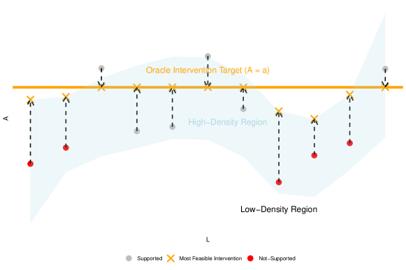
An illustration is provided in Figure 2, where the blue band represents the feasible region for the intervention given the confounders. The most feasible intervention is the closest supported intervention to the oracle intervention of interest, shown in yellow crosses.
3.2.4 Proposal 2: Fix the positivity issue detected in Proposal 1 through novel estimand
Estimand 2 (Feasible) With both definitions of support and substitution intervention function, in Equation (4) and (9), our proposed new estimand is given by:
| (10) |
This can also be written as
| (11) | ||||
Interpretation
Figure 2 illustrates the concept of the most feasible intervention and its interpretation using pseudo-data samples. The dots, shown in red or grey, represent observed data points. We begin by considering an ideal or oracle intervention target , represented by the orange horizontal line, which is intended to evaluate a causal quantity such as the standard causal dose-response curve (CDRC) at this target intervention value . This target quantity, which counterfactually assigns the fixed intervention value to each subject, assumes positivity. However, while this oracle intervention is theoretically appealing, it may not always be supported by sufficient data across all confounder combinations. The shaded blue area in the figure represents the high-density region, where data is abundant, capturing the most likely combinations of confounders and interventions. The observed data points are colored black if the target intervention is within their conditional support, and grey otherwise. The orange crosses indicate the most feasible intervention of each subject for intervention target . If the target intervention is supported, the feasible intervention coincides with ; otherwise, it corresponds to the closest intervention value to that lies within the high-density region.
Violations of the positivity assumption are not merely theoretical concerns but also reflects real-world scenarios where certain interventions are impractical or unrealistic for specific subpopulations. For example, consider drug concentration levels across patients, as discussed in Section 5. Patients with a fast metabolism, who metabolize drugs rapidly, naturally exhibit low drug concentrations even when administered standard doses. For these patients, a high drug concentration target would be unrealistic because it would require doses far beyond what is commonly observed or safely prescribed. While theoretically possible, achieving such concentrations would involve dosing regimens that are rarely practiced due to clinical and practical concerns. This leads to a situation where data corresponding to such high concentrations is either extremely sparse or non-existent, leading to biased causal inferences due to the lack of overlap and making causal conclusions drawn from this target intervention more likely to be unreliable.
The proposed CDRC with the most feasible intervention addresses these issues by adapting the intervention target to stay within regions where data is enough and well-supported. Instead of forcing an unrealistic target that fails to align with real-world conditions, this approach adjusts the intervention based on what is practically achievable and observable within the data. This has two key benefits: first, it reduces bias caused by data sparsity and positivity violations, and second, it ensures that the causal effects being estimated are relevant and actionable in practice.
In contrast to fixed interventions, which risk oversimplifying or misrepresenting causal relationships by imposing uniform targets, the most feasible intervention approach offers a more nuanced and reasonable strategy. It acknowledges the inherent variability in real-world data and adapts the intervention accordingly, leading to more robust, reliable, and meaningful causal inferences that better reflect both the data and the practical realities of clinical and observational settings.
3.3 Trimming
In causal estimation, trimming refers to the process of excluding certain observations from the analysis to improve the accuracy and robustness of estimated treatment effects 6. This is typically done by removing observations that have a low conditional density given the confounders, which can help reduce the impact of outliers or extreme values that may introduce bias or distort the results as given in Equation (12).
| (12) |
where is a critical threshold for the conditional density of the intervention given the confounders.
Estimand 3 (Trimming) The trimming estimand can also be based on the non-overlap ratio defined in Equation (5):
| (13) |
which can be identified by
| (14) |
where is defined as:
| (15) |
Here, and are defined as in Section 2.3.
3.4 Estimation
3.4.1 Causal Estimation
To estimate the standard CDRC in (6), parametric g-formula can be easily applied for the single time-point intervention scenario. Substitution estimators can be constructed to estimate (10) with detailed procedure outlined in Algorithm 1.
-
•
(a) Conditional Density Estimation: Estimate the conditional density model using the observed data .
-
•
(b) High-Density Threshold: For each subject , determine the high-density threshold by computing the -quantile of .
-
•
(a) Estimand 1 (standard): For each intervention , calculate the standard estimand:
-
•
(b) Estimand 2 (feasible): For each intervention , for each subject , evaluate the conditional density as estimated in Step 2(a). Estimate as follows: if is below the high-density threshold , adjust to the nearest feasible value in ; otherwise, retain . Then, calculate the feasible estimand:
-
•
(c) Estimand 3 (trimming): For each intervention , for each subject , evaluate the conditional density as estimated in Step 2(a). Estimate the trimming function as:
Then, calculate the trimming estimand:
3.4.2 Conditional Density Estimation
A key step in this process involves estimating the conditional density function of the intervention given the confounders. Accurate conditional density estimation is critical because it helps quantify the regions where the oracle intervention is supported by the data. Various methods can be employed for this task, including parametric models, non-parametric kernel conditional density estimation 12, and more flexible approaches like the highly adaptive lasso density estimation (Haldensify) 13, 14, 15. Inspired by Haldensify, in this paper we use a specific hazard binning conditional density estimation procedure, which we describe in Appendix Addressing Positivity Violations in Continuous Interventions through Data-Adaptive Strategies and it is similar to the approach described in an earlier proposal 16. These methods allow for the estimation of conditional densities even when the relationship between confounders and interventions is complex or highly non-linear.
4 Simulation Studies
In this section, we examine the proposed methods through three distinct simulation settings. These simulations are designed to provide insight into the performance of the methods under different conditions.
In Simulation 1, we explore how positivity violations exacerbate bias in causal estimates, particularly when the outcome models are misspecified. Simulation 2 examines the impact of positivity violations on causal estimation by comparing scenarios with and without positivity violations. Simulation 3 investigates the methods in a more complex setting, incorporating multiple confounders and intricate data-generating processes.
4.1 Simulation Settings
4.1.1 Simulation 1: Correct model specification versus misspecification under positivity violations
We consider a simple scenario with a single time point where both the intervention and the confounder are normal-distributed shown in Appendix Addressing Positivity Violations in Continuous Interventions through Data-Adaptive Strategies. The simulation study involves three variations that share the same distribution for the confounder and intervention but differ in their outcome functions.
In Simulation 1A, the outcome function is linear. In Simulation 1B, the outcome function is sinusoidal, and in Simulation 1C, it is logarithmic. These two non-linear outcome functions in Simulations 1B and 1C pose a greater challenge for estimation, particularly in regions where data is sparse, i.e. suffering from positivity violations, leading to potential estimation difficulties. In contrast, the linear outcome function in Simulation 1A is expected to be easier to estimate, even in the presence of data sparsity, as the extrapolation will work perfectly.
The primary objective of this simulation design is to evaluate and compare the bias and variability in estimating both the standard CDRC, the proposed CDRC with most feasible intervention, and also the trimming estimand under conditions with positivity violations. This comparison provides insights into the strengths of the proposed most feasible intervention, particularly when outcome functions can not be reliably extrapolated.
4.1.2 Simulation 2: Correct model specification with positivity violations versus no positivity violations
We consider a different scenario with a single time point where the confounder is binary shown in Appendix Addressing Positivity Violations in Continuous Interventions through Data-Adaptive Strategies. The simulation study involves two variations that share the same distribution for the confounder and but differ in their intervention distribution.
In both variations, the intervention distributions given the confounder follow a truncated normal distribution with the same mean value conditional on , but differ in variance. Simulation 2A has a lower variance, leading to greater deviation compared to Simulation 2B. Specifically, for and , the overlap between the distributions of is minimal, indicating a higher degree of positivity violations, as shown in Figure 4a and 4b. The outcome function is a linear combination of and with a small noise term, making it straightforward to estimate and suitable for extrapolation.
The two simulations are designed to compare the estimation of the standard CDRC and the new estimands under conditions of positivity violations (2A) and no positivity violations (2B). This comparison will highlight the performance differences between the three estimands in scenarios where the positivity assumption is either met or violated.
4.1.3 Simulation 3: Simulation study in more complex setting inspired by real data
In this scenario, we consider a complex data-generating process, detailed in Appendix Addressing Positivity Violations in Continuous Interventions through Data-Adaptive Strategies. This process is inspired by real data from the CHAPAS-3 study, an open-label, parallel-group, randomized trial 17, which is further analyzed in Section 5 and follows the setup described in Schomaker et al. 7.
The outcome variable is binary and exhibits a non-linear relationship with the continuous intervention variable, which is modeled using a truncated normal distribution. The simulation aims to validate the proposed approaches in complex scenarios involving intricate distributions and diverse confounders with real-world significance.
4.2 Estimation and Evaluation
4.2.1 Sample Size
For all simulation studies, the sample size is set to .
4.2.2 Causal Parameters
4.2.3 Causal Estimation
For simulation studies 1 and 2, we estimate using the standard parametric g-computation plug-in estimator. For simulation 3, we employed the semi-parametric version. The specific details of the estimation are given in the Algorithm 1.
4.2.4 Conditional Density Estimation
For simulation 1, we performed parametric conditional density estimation via linear regression. In simulation 2, we used non-parametric kernel conditional density estimation, offered in R package np 12. For simulation 3, we implemented super learner based conditional density estimation, as described in Appendix Addressing Positivity Violations in Continuous Interventions through Data-Adaptive Strategies.
4.2.5 Bias Metrics
To evaluate the estimation bias of each estimand, all Monte Carlo simulations are based on runs.
We define
with
and represents the result of each Monte Carlo run.
4.3 Results
4.3.1 Simulation 1
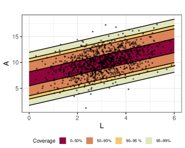
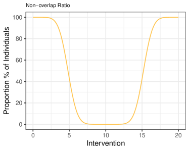
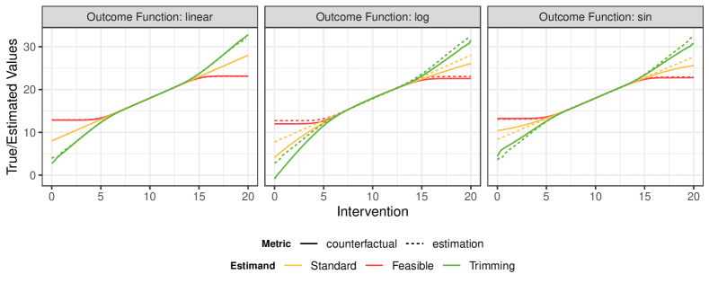
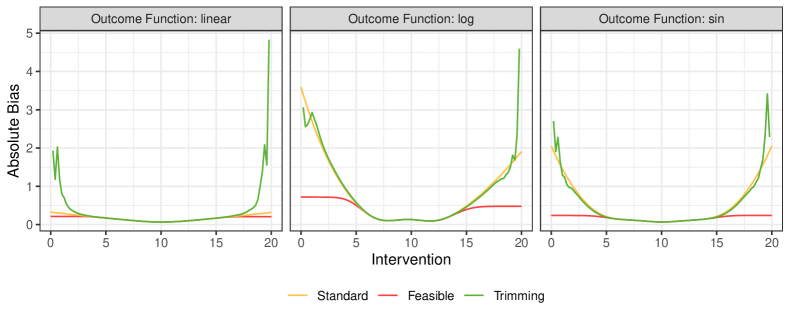
Figure 3a illustrates the estimated conditional distribution and coverage levels at , , , and , overlaid with a scatter plot of observed data from a single simulation run. Areas outside these regions highlight rare combinations of and in observation, reflecting data sparsity. Using the diagnostic approach from Section 2.3, we identify positivity violations, as shown in Figure 3b.
Figure 3b presents the non-overlap ratio, a diagnostic metric quantifying the proportion of the population for which specific interventions are infeasible at a coverage level. This ratio, ranging from to , reveals a clear pattern: in the central region, nearly all interventions have a non-overlap ratio of zero, indicating good feasibility. In contrast, the ratio rises sharply at the extremes, indicating that extremely small or large interventions are largely infeasible.
Together, Figures 3a and 3b show that certain interventions are rare or infeasible for subsets of the population. Even theoretically feasible, interventions may lack sufficient data for accurate estimation, underscoring the importance of our proposed feasible intervention framework.
Figure 3c examines the impact of non-overlap and model misspecification on the estimation of three estimands under linear, logarithmic, and sinusoidal outcome functions. In regions where the non-overlap ratio is near zero, counterfactual estimates for the three estimands are nearly identical across all outcome functions, as intended by the simulation design. At the extremes, however, the estimands diverge. The CDRC with the most feasible intervention establishes practical thresholds, avoiding unrealistic extrapolation into sparsely supported regions. The trimming estimand, by contrast, restricts the population to those for whom the intervention is feasible.
For linear outcome functions (Figure 3c, left), extrapolation is highly accurate, resulting in minimal absolute bias across all estimands (Figure 3d, left). However, for logarithmic and sinusoidal functions (Figure 3c, middle and right), extrapolation accuracy diminishes in sparsely supported regions, increasing absolute bias for all estimands (Figure 3d, middle and right).
The most feasible intervention consistently achieves lower absolute bias, particularly when outcome functions are misspecified and extrapolation is unreliable. By focusing on well-supported regions, it avoids large biases and maintains robust estimates even in areas with low non-overlap. Conversely, the trimming estimand exhibits high variability and substantial absolute bias, even in the linear case, due to its restrictive population definition.
These results emphasize the benefits of the most feasible intervention approach, which balances estimation reliability and accuracy by limiting extrapolation only in feasible intervention regions.
4.3.2 Simulation 2
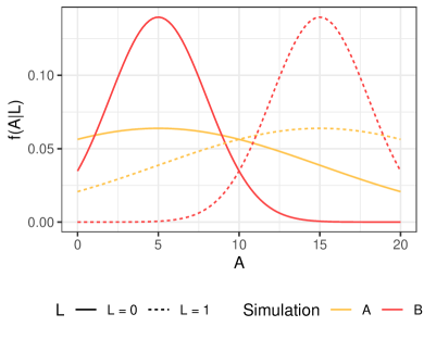
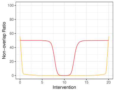
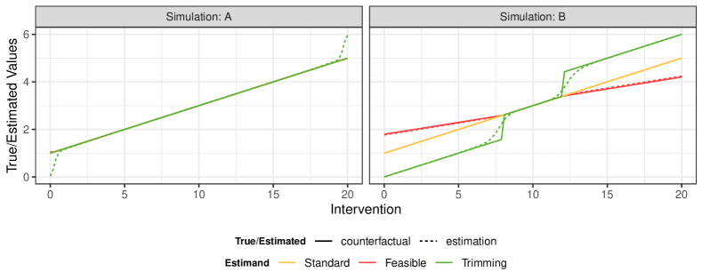
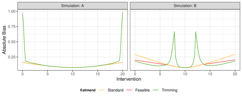
Figure 4a illustrates the conditional distribution of given . In Simulation 2A, this distribution is more concentrated, with lower variance compared to Simulation 2B. This distribution design increases the chance of non-overlap in Simulation 2B, as shown in Figure 4b.
Figure 4b presents the non-overlap ratio for each intervention. In Simulation 2B, the ratio is lower in the central region but rises sharply to 50% in the extreme intervention regions due to the divergence between the conditional distributions of for and . In contrast, Simulation 2A exhibits generally low non-overlap ratios across intervention values, except near the boundaries. This difference arises because, in Simulation 2B, the intervention distributions for and are distinct, whereas in Simulation 2A, they are more similar, exhibiting higher overlap.
Figure 4c shows the true estimand values for both the standard CDRC,the CDRC with the most feasible intervention and trimming estimand. In Simulation 2A, where non-overlap is absent, the three true curves are nearly identical because the intervention is feasible for all individuals. However, in Simulation 2B, the estimands diverge outside the central region, as the most feasible intervention shifts toward the center due to limited feasibility at extreme values, and the trimming estimand exhibits more radical counterfactual shifts. For all three curves, the estimates are very close to the true values, as the true outcome function is designed to be straightforward.
Figure 4d compares the absolute bias between Simulations 2A and 2B. Compared to Simulation 2A, Simulation 2B exhibits positivity violation issues, leading to higher absolute bias for all estimands, particularly in regions with high non-overlap. Nonetheless, the most feasible intervention shows lower bias under both conditions compared to the standard estimand and does not exceed the bias level of the standard estimand when positivity violations are minimal, as observed in Simulation 2A. The trimming estimand performs well at times, but it is unstable in certain areas.
4.3.3 Simulation 3
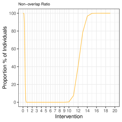
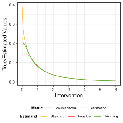
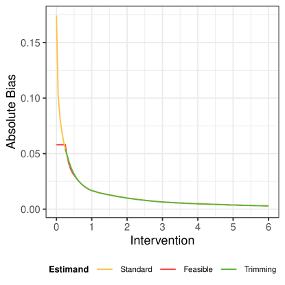
Figure 5a illustrates the non-overlap ratio in the range of , which shows a sharp increase at very low intervention values below and above . In the following, we focus on the intervention region of .
Figure 5b presents the true and estimated values for the three estimands. In regions where the non-overlap ratio is zero, the three estimands are indistinguishable. However, the standard estimand increases dramatically near an intervention value of . As indicated by the non-overlap ratio, such values are nearly impossible to intervene on. In the data-generating process (see Appendix Addressing Positivity Violations in Continuous Interventions through Data-Adaptive Strategies), the truncated normal distribution excludes values below , causing the true curve of the trimmed estimand to terminate near this intervention value. This indicates that intervention values below are strictly infeasible, representing a theoretical positivity violations and thus making counterfactual curve of trimming estimand unidentifiable below that threshold. Unlike the standard estimand, the proposed most feasible intervention estimand does not exhibit extreme values in regions with very low intervention, making it more robust and less prone to positivity issues.
Figure 5c demonstrates that the most feasible intervention estimand consistently achieves lower absolute bias, particularly in regions with positivity violations. It effectively avoids large biases and maintains robust estimates even in areas with low or no non-overlap. While the trimming estimand also reduces bias, it becomes not estimable when the non-overlap ratio approaches , as no samples are available in such scenarios.
These findings underscore the practical utility of the proposed methods for complex data-generating processes with real-world significance.
5 Data Analysis
We demonstrate our approach using pharmacoepidemiological data of HIV-positive children from the CHAPAS-3 trial, which enrolled children aged 1 month to 13 years in Zambia and Uganda 17, 18. We focus on those 125 children who received efavirenz as part of antiretroviral therapy, together with both lamivudine and either stavudine, zidovudine, or abacavir.
In line with previous studies 19, 20, 21, we are interested in how counterfactual viral failure probabilities (VLt), defined as a viral load exceeding copies/mL, vary as a function of different efavirenz concentrations (EFVt, defined as the plasma concentration (in mg/L) measured hours after dosing). Briefly, different patients who take the same efavirenz dose, may still have different drug concentrations in their blood, for example because of their individual metabolism. Patients exposed to suboptimal concentrations may experience negative outcomes and one may ask at which concentration level antiretroviral activity is too low to guarantee suppression for most patients. Thus, one may be interested in the concentration-response curve mg/L; although it is known that not every child can achieve every possible concentration level, depending on their clinical and metabolic profile and thus positivity violations may be likely 7.
For illustration, we use baseline data and data from the scheduled visit at (weeks). The relevant part of the assumed data-generating process is, in line with previous studies 21, 22, 7, summarized by the directed acyclic graph (DAG) in Figure 6:
Our analysis illustrates the ideas based on a complete case analysis of all measured variables at (weeks) represented in the DAG . The analysis was conducted using three coverage levels for detecting non-overlap: , , and . Our target estimand is the standard causal concentration-response curve, defined in Section 3.1. We compare this estimand to the proposed estimand with most feasible intervention strategy, described in Section 3.2.4, as well as the trimming estimand in Section 3.3. The estimation process closely follows the detailed methodology described in Section 3.4 and algorithm outlined in Algorithm 1. Bootstrap resampling was used to estimate compatibility intervals.
5.1 Results
The results of the analysis are presented in Figure 7 and are discussed in two parts: (1) diagnostics assessing the extent of positivity violations based on intervention values, and (2) estimates of three estimands.
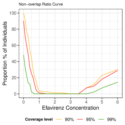
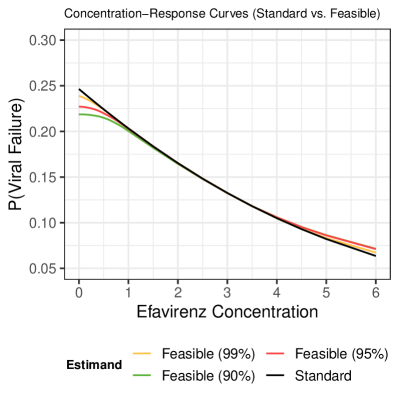
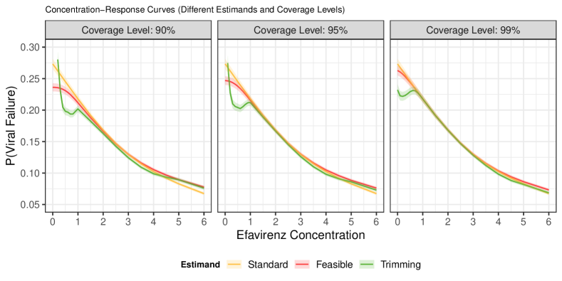
Figure 7a illustrates the proposed non-overlap ratios as diagnostics for identifying positivity violations in continuous interventions. These ratios, calculated as a function of the intervention , represent the proportion of the population where the intervention is not feasible, based on 3 coverage levels of non-overlap detection.
The non-overlap ratios remain low across all coverage levels within the central intervention range (approximately to mg/L), suggesting minimal violations of positivity in this region and supporting reliable causal estimation. However, at the boundaries of the intervention range—below mg/L or above mg/L—the ratios increase, indicating more frequent violations. Notably, near mg/L, the non-overlap ratio rises sharply, signaling strong violations of the positivity assumption, consistent with the fact that concentrations this low are virtually impossible to observe.
Figure 7b show the estimated curves of the most feasible intervention across three coverage levels compared with the standard causal concentration-response curve. In regions with positivity violations, using the most feasible intervention strategy differs from the CDRC, while closely aligning with standard estimates in well-supported regions. This means whenever a concentration value seems unlikely or implausible, we do not enforce this intervention but rather use the closest value that is possible. This may happen, for example, if there are patients with a very slow metabolism who will never be able to clear the drug fast enough to ever achieve concentrations under mg/L.
Figure 7c compares all estimated causal curves across three coverage levels. As the coverage level increases, more positivity violations are tolerated for both the feasible intervention and triming estimands. However, the triming estimand exhibits instability in regions with strong positivity violations, suggesting that it may not be the optimal approach in this analysis.
6 Conclusion
Positivity violations are a common issue with continuous interventions, presenting significant challenges when the outcome function cannot be extrapolated reliably from observed to unobserved regions. These violations occur when certain values of the intervention are not adequately represented in the data, leading to a lack of support and, consequently, unreliable estimations.
One of the key consequences of positivity violations is an increase in absolute bias. This issue persists even when the underlying model is correctly specified. In essence, the model’s ability to provide accurate estimates is compromised not only by incorrect specifications but also by the absence of sufficient data in certain regions of the intervention space, which implies addressing positivity violations is not a problem that can be resolved merely by employing robust estimators against misspecification.
Estimating the standard causal dose-response curve (CDRC), an idealized causal representation of the relationship between the intervention and outcome, becomes particularly complex when the range of interventions is extensive. The broad spectrum of interventions can exacerbate the difficulty of making accurate estimations, as it requires the model to reliably estimate across a wide range of values, including those not well-represented in the data.
To address this challenge, we propose using a data-adaptive intervention as a novel strategy to construct a new estimand that tackles positivity issues. The key idea is to adhere as closely as possible to the actual CDRC, deviating only for individuals where the target intervention is clearly infeasible based on the data. In such cases, we substitute the intervention with the most feasible value, ensuring the interpretation remains meaningful: we either apply the intervention of interest or the nearest feasible alternative. By focusing on a more practical and adaptive range of interventions, this approach reduces bias and improves robustness. Consequently, the resulting causal dose-response curve accurately reflects relationships where sufficient data exists, enhancing both precision and interpretability.
In summary, while positivity violations present significant challenges, careful selection of estimands can substantially mitigate variability and enhance the interpretability of the estimates. Future research should explore adapting the concept of the data-adaptive intervention to longitudinal settings, as well as developing and applying different estimators and estimation methods to further refine and validate these approaches. Additionally, there is considerable room for improvement in defining the practical support and refining substitution intervention functions, especially in addressing limitations related to the reliance on conditional density estimation.
*Acknowledgments We sincerely thank the CHAPAS-3 trial team for their support, valuable advice on the illustrative data analysis, and for providing access to their data.
We extend our special thanks to Sarah Walker, Di Gibb, Andrzej Bienczak, David Burger, Elizabeth Kaudha, Paolo Denti, and Helen McIlleron for valuable advice regarding the data and continuous support. Additionally, we are deeply grateful to Iván Díaz for his constructive and insightful feedback on earlier versions of this manuscript.
The research is supported by the German Research Foundations (DFG) Heisenberg Program (grants 465412241 and 465412441).
References
- 1 Imbens GW, Rubin DB. Causal inference for statistics, social, and biomedical sciences: An introduction. Cambridge University Press, 2015.
- 2 Hernán MA, Robins JM. Causal inference: What if. Boca Raton: Chapman & Hall/CRC, 2020.
- 3 Zivich PN, Cole SR, Westreich D. Positivity: Identifiability and estimability. arXiv preprint arXiv:2207.05010. 2022.
- 4 Petersen ML, Porter KE, Gruber S, Wang Y, Van Der Laan MJ. Diagnosing and responding to violations in the positivity assumption. Statistical methods in medical research. 2012;21(1):31–54.
- 5 Westreich D, Cole SR. Invited commentary: positivity in practice. American journal of epidemiology. 2010;171(6):674–677.
- 6 Crump RK, Hotz VJ, Imbens GW, Mitnik OA. Dealing with limited overlap in estimation of average treatment effects. Biometrika. 2009;96(1):187–199.
- 7 Schomaker M, McIlleron H, Denti P, Díaz I. Causal Inference for Continuous Multiple Time Point Interventions. Statistics in Medicine. 2024;43(28):5380-5400.
- 8 Moccia C, Moirano G, Popovic M, et al. Machine learning in causal inference for epidemiology. European Journal of Epidemiology. 2024:1–12.
- 9 Haneuse S, Rotnitzky A. Estimation of the effect of interventions that modify the received treatment. Statistics in medicine. 2013;32(30):5260–5277.
- 10 Díaz I, Williams N, Hoffman KL, Schenck EJ. Nonparametric causal effects based on longitudinal modified treatment policies. Journal of the American Statistical Association. 2023;118(542):846–857.
- 11 Hyndman RJ. Computing and graphing highest density regions. The American Statistician. 1996;50(2):120–126.
- 12 Hayfield T, Racine JS. Nonparametric econometrics: The np package. Journal of statistical software. 2008;27:1–32.
- 13 Hejazi NS, Benkeser D, Díaz I, van der Laan MJ. Efficient estimation of modified treatment policy effects based on the generalized propensity score. 2022.
- 14 Hejazi NS, van der Laan MJ, Benkeser DC. haldensify: Highly adaptive lasso conditional density estimation in R. Journal of Open Source Software. 2022. doi: 10.21105/joss.04522
- 15 Hejazi NS, Benkeser DC, van der Laan MJ. haldensify: Highly adaptive lasso conditional density estimation. https://github.com/nhejazi/haldensify; 2022. R package version 0.2.5
- 16 Díaz Muñoz I, Laan v. dMJ. Super learner based conditional density estimation with application to marginal structural models. The international journal of biostatistics. 2011;7(1):0000102202155746791356.
- 17 Mulenga V, Musiime V, Kekitiinwa A, et al. Abacavir, zidovudine, or stavudine as paediatric tablets for African HIV-infected children (CHAPAS-3): an open-label, parallel-group, randomised controlled trial. The Lancet Infectious diseases. 2016;16(2):169-79.
- 18 Abongomera G, Cook A, Musiime V, et al. Improved Adherence to Antiretroviral Therapy Observed Among HIV-Infected Children Whose Caregivers had Positive Beliefs in Medicine in Sub-Saharan Africa. Aids and Behavior. 2017;21(2):441-449.
- 19 Bienczak A, Denti P, Cook A, et al. Plasma efavirenz exposure, sex, and age predict virological response in HIV-infected African children. JAIDS Journal of Acquired Immune Deficiency Syndromes. 2016;73(2):161–168.
- 20 Bienczak A, Denti P, Cook A, et al. Determinants of virological outcome and adverse events in African children treated with paediatric nevirapine fixed-dose-combination tablets. Aids. 2017;31(7):905–915.
- 21 Schomaker M, Denti P, Bienczak A, et al. Determining Targets for Antiretroviral Drug Concentrations: a Causal Framework Illustrated with Pediatric Efavirenz Data from the CHAPAS-3 Trial. Pharmacoepidemiology and Drug Safety. 2024;in press.
- 22 Holovchak A, McIlleron H, Denti P, Schomaker M. Recoverability of Causal Effects in a Longitudinal Study under Presence of Missing Data. Biostatistics. 2024;in press, https://arxiv.org/abs/2402.14562.
- 23 Léger M, Chatton A, Le Borgne F, Pirracchio R, Lasocki S, Foucher Y. Causal inference in case of near-violation of positivity: comparison of methods. Biometrical Journal. 2022;64(8):1389–1403.
- 24 Hejazi NS, Laan v. dMJ, Benkeser D. haldensify: Highly adaptive lasso conditional density estimation inR. Journal of Open Source Software. 2022;7(77):4522.
Additional Information
In the literature, positivity violations are usually classified into two types: structural and practical, typically for binary interventions 3, 4, 5. We could formulate these definitions for continuous interventions similarly.
Near positivity violations This occurs when the positivity assumption is almost violated. In these situations, the probability of receiving certain treatment levels given specific confounder combinations is very close to zero but not exactly zero. Although this is not a complete violation, it has similar practical implications. Near positivity violations affect the bias and precision of causal estimation 23, leading to unreliable treatment effect estimates in these regions due to sparse data. Common causal methods are particularly sensitive to such violations 23.
Structural positivity violations A structural positivity violation occurs when, due to the structure of the data or the study design, certain groups of individuals (defined by their confounders) have no chance of receiving some treatment value. In such cases, we simply define that .
Practical positivity violations Also known as stochastic positivity violations, it occurs when a treatment, although clinically possible for patients with specific confounders, is not observed in the data, which results in .
However, for continuous interventions, defining practical positivity violations is more complex because we cannot observe the exact intervention value, and depends on the density function estimation.
Positivity violations, both structural and practical violations, have a non-negligible impact on plug-in estimation of Equation 6. In the process of estimating the causal CDRC via the standard parametric g-formula, the conditional expectation , typically as a (generalized) linear regression, is estimated by minimizing the expectation of square loss:
| (16) | ||||
The standard causal CDRC is identified by:
| (17) |
The Mean Squared Error (MSE) of is given by:
| (18) |
We apply the estimator in Equation (16) to the observed data . When the conditional density are very small, indicating that certain treatment-confounder combinations are sparse or even impossible, their contribution to the overall loss function is minimal. However, during the estimation of the causal dose-response curve, the MSE (Equation 18) from these rare treatment-confounder combinations can be significantly amplified across the entire population.
In other words, deriving the outcome model from observed data where rare treatment-confounder combinations are poorly represented leads to inaccurate extrapolations in these sparse regions. When this model is applied to the entire population, the variability of the estimation increases dramatically.
Simulation Parameters
Data Generating Process for Simulation 1
Simulation 1A: Linear outcome function
Simulation 1B: Sinusoidal outcome function
Simulation 1C: Logarithmic outcome function
Data Generating Process for Simulation 2
Simulation 2A
Simulation 2B
Data Generating Process for Simulation 3
| Sex | |||
| Genotype | |||
| Age | |||
| NRTI | |||
| MEMS | |||
| Weight | |||
| CoMo | |||
| Dose | |||
| EFV | |||
| VL | |||
The distribution represents a truncated normal distribution, where and are the truncation thresholds. Values less than are replaced with random draws from a distribution, while values greater than are replaced with random draws from a distribution. Here, denotes a continuous uniform distribution.
Estimate the Conditional Density via Hazard Binning
Consider discretizing the observed variable into bins using an appropriate binning procedure. Given this, we can estimate the probability of falling into the interval , using a standard classification model. Within each bin , the density is assumed to undergo a uniform transformation, leading to the following expressions:
To obtain the density, we can apply either parametric or non-parametric estimation to the hazard model and then transform the results into a density for each bin. This approach is adapted from Haldensify, proposed by Nima S. Hejazi et al. 24, 15, 14, and it is similar to the approach described in an earlier proposal 16.