Corresponding author: E-mail: ]shubh.iiitj@gmail.com
Thermal phototactic bioconvection in an isotropic porous medium heated from above
Abstract
This study investigates thermal phototactic bioconvection in an isotropic porous medium using the Darcy-Brinkman model. The top boundary of the medium is exposed to normal collimated light and subjected to heating. A linear analysis of bio-thermal convection is performed using a fourth-order accurate finite difference scheme, employing Newton-Raphson-Kantorovich iterations for both rigid-free and rigid-rigid boundary conditions. The effects of the Lewis number, Darcy number, and thermal Rayleigh number on bioconvective processes are examined and presented graphically. The findings reveal that increasing the thermal Rayleigh number stabilizes the suspension, whereas a higher Lewis number enhances instability.
I INTRODUCTION
Bioconvection is a fluid dynamics phenomenon driven by the collective motion of self-propelled microorganisms that are slightly denser than their surrounding fluid. This process plays a crucial role in various biological and industrial applications Platt (1961); Pedley and Kessler (1992); Hill and Pedley (2005); Bees (2020); Javadi et al. (2020). Motile microorganisms, such as algae and bacteria, generate density variations as they respond to external stimuli, a behavior known as taxis, leading to convective instability. Key examples of taxis include phototaxis, gravitaxis, gyrotaxis, chemotaxis, and thermotaxis. Understanding bioconvection is particularly relevant in environmental science, biotechnology, and engineering, where it influences nutrient transport, bioreactor efficiency, and microbial ecology.
Early research primarily focused on suspensions under isothermal conditions. However, many microorganisms, particularly thermophiles inhabiting hot springs, thrive in environments with significant temperature variations Kuznetsov (2005); Alloui et al. (2006); Nield and Kuznetsov (2006). Among the various types of taxis influencing microbial movement, phototaxis (response to light) and thermotaxis (response to temperature gradients) play a crucial role in shaping bioconvective patterns Rajput and Panda (2025a). While substantial research has been dedicated to phototactic and gravitactic bioconvection in non-porous media, thermal bioconvection in porous media saturated with algal suspensions remains relatively under-explored. The presence of a porous matrix introduces additional complexities, such as flow resistance and modified convective dynamics, making it a critical area of study for both natural ecosystems and industrial fluid systems.
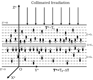
The formation and characteristics of bioconvection patterns influenced by phototaxis depend on various environmental light conditions, including direct and oblique collimated solar irradiation Wager (1911); Kitsunezaki et al. (2007); Kessler (1985); Williams and Bees (2011); Kessler (1986); Kessler and Hill (1997); Vincent and Hill (1996). High-intensity light can either disrupt established patterns or inhibit their development Kessler (1985); Williams and Bees (2011); Kessler (1989). Variations in illumination levels contribute to changes in the spatial structure and size of these patterns. These alterations can be attributed to specific mechanisms. Photosynthetic microorganisms exhibit directional movement in response to light intensity. When the intensity remains below a critical threshold , they exhibit positive phototaxis, migrating toward brighter regions. However, when surpasses , they exhibit negative phototaxis, moving toward lower light intensities to avoid potential damage. This behavior results in the accumulation of microorganisms in regions where , forming structured bioconvective patterns (see Fig. 1) Häder (1987). Additionally, the process of light absorption significantly influences pattern formation by affecting the spatial distribution of microorganisms within the suspension Ghorai et al. (2010); Straughan (1993).
Over the years, significant progress has been made in understanding the mechanisms of bioconvection. Early research primarily focused on gravitactic microorganisms, where the swimming behavior of dense motile microbes was analyzed to determine the instability conditions that lead to convective flow Kessler (1989). Later, studies on phototactic bioconvection emerged, emphasizing the interactions between microbial responses to light intensity, absorption effects, and microorganism concentration Vincent and Hill (1996). Ghorai and Hill Ghorai and Hill (2005) extended this research by developing two-dimensional phototactic bioconvection models, emphasizing the role of shading effects. Further studies by Ghorai et al. Ghorai et al. (2010) investigated phototactic bioconvection in isotropically scattering algal suspensions, while Panda and Singh Panda and Singh (2016) analyzed its onset in a two-dimensional system with free side walls. The scattering properties of algae, influenced by their shape and size, affect light propagation. Early studies suggested that algae predominantly scatter light in the forward direction. To explore the role of forward scattering at the onset of bioconvection, Ghorai and Panda Ghorai and Panda (2013) developed a mathematical model. Panda et al. Panda et al. (2016) later investigated the combined effects of diffuse and collimated light fluxes in an isotropic scattering medium, while Panda Panda (2020) extended this research to anisotropic scattering media. Further work by Panda et al. Panda et al. (2022) examined the impact of oblique collimated flux on bioconvective instability in algal suspensions, whereas Panda and Rajput Panda and Rajput (2023) studied the combined effects of diffuse and oblique collimated flux in a uniformly (isotropic) scattering suspension. Recent studies by Rajput and Panda Rajput and Panda (2024, 2025b) focused on the influence of a diffuse flux alone on photo-bioconvective instability in an isotropically scattering suspension with both rigid and free top walls. More recently, the same authors Rajput and Panda (2025c, d) analyzed bioconvective instability in an anisotropic suspension within the same geometric framework.
In addition to phototaxis, thermal effects on bioconvection have attracted considerable interest due to their influence on microorganism motility, metabolic activity, and fluid density variations. Kuznetsov Kuznetsov (2006) investigated thermo-bioconvection in a shallow porous layer heated from below, highlighting the role of thermal Rayleigh numbers in convective instability. Sheremet and Pop Sheremet and Pop (2014) examined thermo-bioconvection within a square porous cavity, focusing on the behavior of oxytactic microorganisms in the presence of thermal gradients. Zhao et al. Zhao et al. (2019) explored the impact of porous matrices on thermal bioconvection, providing insights into heat transfer mechanisms governing bioconvective flows. Further studies have examined external influences on thermal bioconvection. Biswas et al. Biswas et al. (2021) analyzed the role of magnetic fields in thermo-bioconvection, proposing new strategies for regulating convection in bio-suspensions. More recently, Kopp and Yanovsky Kopp and Yanovsky (2024) incorporated weakly nonlinear stability analysis to investigate bio-thermal convection under rotation, gravity modulation, and heat sources, contributing to a deeper theoretical understanding of the phenomenon.
Despite significant advancements, the intricate interplay between thermal effects, porous media, and phototaxis in bioconvection remains under-explored. This study seeks to bridge these gaps by formulating a mathematical model for thermal bioconvection in a porous medium. The model incorporates the Navier-Stokes equations with the Boussinesq approximation, a microorganism conservation equation, and an energy equation. The primary objectives include analysing stability conditions, examining the influence of various physical parameters on convection onset, and assessing practical implications for biotechnological applications. These applications span diverse fields, including biofuel production, water filtration, and environmental remediation.
This paper is structured as follows: Section 2 introduces the mathematical formulation, defining the governing equations and boundary conditions. Section 3 discusses the steady-state solution, outlining the equilibrium conditions. Section 4 presents the linear stability analysis, which establishes the criteria for instability. Section 5 describes the numerical solution methodology, followed by Section 6, which provides numerical results and examines the influence of various parameters on bioconvection behavior. Finally, Section 7 summarizes the key findings and proposes potential directions for future research.
II Problem formulation
A porous medium filled with an algal suspension is considered, confined between two horizontal planes located at and , extending infinitely in the horizontal directions. The study examines two boundary configurations: (i) a free-rigid setup, where the upper boundary is stress-free and the lower boundary is rigid, and (ii) a rigid-rigid setup, where both boundaries are rigid. The system is illuminated by collimated irradiation from above, while thermal effects are incorporated by applying heat at the bottom boundary. To ensure microbial viability and preserve phototactic behavior, the imposed temperature variations are assumed to be minimal. The upper boundary is maintained at a constant temperature , while the lower boundary is kept at .
II.1 THE GOVERNING EQUATIONS
A dilute, incompressible suspension of phototactic microorganisms is considered. The governing equations are formulated based on the models introduced by Kuznetsov Kuznetsov (2005) and Vincent and Hill Vincent and Hill (1996). It is assumed that the heating process does not alter the microorganisms’ phototactic behavior, including their swimming orientation and velocity.
Each microorganism is characterized by a volume and a density contrast relative to the fluid density . The mean velocity of the suspension is represented by . The fundamental equations governing this system are given as follows:
Continuity equation
| (1) |
Momentum equation
| (2) |
Here, , , , and represent the hydrostatic pressure, viscosity, thermal expansion coefficient, and unit vector in the vertical direction. Also and denote the porosity and permeability of the medium.
Cell conservation equation
| (3) |
where the total flux is
The thermal energy equation
| (4) |
where the thermal conductivity and the volumetric heat capacity of water are denoted by and , respectively.
The cell flux formulation is based on the assumption that microorganisms are purely phototactic, neglecting viscous torque effects in horizontal swimming. The diffusion tensor is considered isotropic, Ghorai and Hill (2005).
Light Intensity Equation:
| (5) |
Here, is the vector from the microorganism to the light source, is the incident light intensity, represents the microorganism concentration, and is the extinction coefficient. This formulation is based on the Lambert-Beer law, considering only absorption by microorganisms while neglecting scattering.
II.2 SWIMMING ORIENTATION
The mean swimming direction of cells is represented by . For many microorganism species, the swimming speed remains independent of factors such as illumination, position, time, and direction Hill and Häder (1997). The average swimming speed is denoted by . Consequently, the mean velocity of the swimming cells is given by:
The mean swimming direction, , is expressed as:
| (6) |
where is the unit vector along the vertical -axis, and is the phototaxis function, defined as:
The mean swimming direction becomes zero when or when .
For an algal suspension exposed to uniform illumination, the light intensity is influenced by the concentration of cells, as those closer to the light source cast shadows on those farther away. Thus, the light intensity at a given position within the suspension is determined by:
| (7) |
II.3 BOUNDARY CONDITIONS
In this analysis, results will be presented for both free and rigid upper horizontal boundaries. In experimental settings, the lower boundary is typically rigid, while the upper boundary may be either free or rigid.
The boundary conditions governing the system are given by
| (8) |
| (9) |
For a rigid boundary
| (10) |
For a free boundary
| (11) |
Also, the thermal boundary conditions
| (12) |
| (13) |
II.4 SCALING OF THE EQUATIONS
The equations have been scaled following the parameters used by Ghorai & Hill Ghorai and Hill (2005) and Kuznetsov Kuznetsov (2005). The both dimensional and nondimensional variables are shown by same symbol. The governing bioconvection equations in dimensionless form are
| (14) |
| (15) |
| (16) |
where
and
| (17) |
The non-dimensional parameters considered in this study include the Prandtl number, and the dimensionless swimming speed is given by . The bio-convective Rayleigh number is defined as and the thermal Rayleigh number is given by . The basic density Rayleigh number is and the Lewis number is defined as . Additionally, the Darcy number, which characterizes the permeability of the porous medium, is given by .
The dimensionless form of the light intensity at position is
| (18) |
where is the non-dimensional extinction coefficient.
After scaling, the boundary conditions are given by
| (19) |
| (20) |
For a rigid boundary
| (21) |
whereas for a free boundary
| (22) |
Also, the thermal boundary conditions
| (23) |
| (24) |
III The steady solution
| (25) |
The steady-state concentration satisfies the equation
| (26) |
where represents the phototaxis function evaluated at steady-state light intensity , given by
| (27) |
Introducing the transformation , Eq. (27) is rewritten as
| (28) |
The boundary conditions for are given by
| (29) |
| (30) |
The temperature profile is governed by
| (31) |
| (32) |
Next, Eq. (28) along with boundary conditions (29) and (30), define a boundary value problem which is solved by using a shooting method.
In this study, the phototaxis function is modeled as
| (33) |
where . The parameter is related to , and its specific form depends on the type of microorganisms considered.
IV The perturbed system
To analyze the stability of the system, a small perturbation of amplitude (where ) is introduced to the steady-state solution, leading to
| (34) |
where .
Substituting these perturbed variables into Eqs. (1)–(4) and retaining only terms of order results in the following linearized system
| (35) |
| (36) |
| (37) |
| (38) |
If , the perturbed light intensity , after expanding and retaining terms of order , is given by
| (39) |
Expanding to first order in gives
| (40) |
To eliminate and the horizontal components of , we take the double curl and extract the vertical component, reducing Eqs. (35)– (38) to three equations for , , and . These are then expressed in normal modes as
| (42) |
Thus, the governing equations simplify to
| (43) |
| (44) |
| (45) |
The boundary conditions are
| (46) |
| (47) |
For a rigid upper boundary, the condition in Eq. (47) is replaced by
| (48) |
The thermal boundary conditions are
| (49) |
The system Eqs. (IV)–(45) form an eigenvalue problem for , determining the stability of the perturbations.
Introducing a new variable:
The perturbed equations, rewritten using , take the form
| (50) |
| (51) |
| (52) |
The boundary conditions are
| (53) |
| (54) |
Additionally, an extra boundary condition
| (57) |
V SOLUTION technique
The stability analysis of the system described by Eqs. (50)–(52) is carried out using a fourth-order finite difference scheme combined with Newton-Raphson-Kantorovich (NRK) iterations Cash and Moore (1980). This numerical technique allows for the evaluation of the growth rate, Re, and the construction of neutral stability curves in the -plane under different parameter conditions, where can take values or .
The neutral stability curve, expressed as , contains an infinite sequence of branches indexed by , each corresponding to a distinct solution of the linear stability problem. The most unstable mode is associated with the lowest value, defining the critical solution as , where the critical Rayleigh number corresponds to either or .
VI NUMERICAL RESULTS
This study systematically investigates the influence of thermal effects on algal suspensions by exploring the parameter space. A controlled approach is adopted, where specific parameters remain fixed while others are varied to assess their impact on bioconvection onset. To maintain consistency, the governing parameters are set as and , while different values of other parameters are considered to analyse their effects.
To account for variations in light absorption properties, two cases are examined: and . Furthermore, the critical light intensity, , is chosen such that the steady-state condition occurs at different depths within the suspension, specifically at the top, three-quarters, or mid-height. The primary objective of this analysis is to determine the critical bioconvective Rayleigh number, , as a function of the thermal Rayleigh number, , providing insights into the stability conditions under varying thermal influences.
VI.1
The results of this section is divided into two categories based on the top surface conditions.
VI.1.1 WHEN TOP SURFACE IS STRESS FREE
Figure 2 shows the neutral curves for different values of the thermal Rayleigh numbers. Here the other parameters , and are fixed. It is clear that the as the thermal Rayleigh number increases, the critical bioconvective Rayleigh number increases. Thus the suspension becomes more stable as the thermal Rayleigh number increases.

Also, Fig. 3 illustrates the neutral curves for different values of the Lewis numbers. Here the other parameters , and are fixed. The critical bioconvective Rayleigh number decreases as the thermal Rayleigh number increases.

VI.1.2 WHEN TOP SURFACE IS RIGID
Figure 4 shows the neutral curves for different values of the thermal Rayleigh numbers. Here the other parameters , and are fixed. It is clear that the as the thermal Rayleigh number increases, the critical bioconvective Rayleigh number increases. Thus the suspension becomes more stable as the thermal Rayleigh number increases.

Also, Fig. 3 illustrates the neutral curves for different values of the Lewis numbers. Here the other parameters , and are fixed. The critical bioconvective Rayleigh number decreases as the thermal Rayleigh number increases.

VII Conclusion
This study presents a novel thermal phototactic bioconvection model that integrates thermal effects into the dynamics of bioconvective systems in a porous medium. The suspension is exposed to collimated light from above and also subjected to heating from the same side. The primary objective is to examine how thermal variations impact the onset and behavior of phototactic bioconvection in a porous environment. The numerical results, obtained through a linear stability analysis under specific control parameters, are summarized below.
The accumulation of algal cells within the suspension forms a sublayer, whose position is governed by the critical light intensity. When the critical intensity matches the incident light intensity, cells cluster at the top; as the critical intensity decreases, this aggregation shifts downward. Moreover, a reduction in light intensity corresponds to a decrease in the maximum concentration at the sublayer.
The linear stability analysis reveals both steady and oscillatory solutions, with oscillations becoming particularly pronounced when the microorganism layer is positioned around three-quarters of the suspension height, dictated by the critical light intensity. Notably, these oscillations transition to a stationary state as the critical thermal Rayleigh number increases. As the thermal Rayleigh number increases, the critical bioconvective Rayleigh number increase. On the other hand, the critical bioconvective Rayleigh number decreases as the Lewis number increases. Thus the suspension become stable (unstable) as the thermal Rayleigh number (Lewis number) increases.
CONFLICT OF INTEREST
The authors state that they have no conflicts of interest.
DATA AVAILABILITY
The findings of this study are supported by the data contained within this article.
REFERENCES
References
- Platt (1961) J. R. Platt, Science 133, 1766 (1961).
- Pedley and Kessler (1992) T. J. Pedley and J. O. Kessler, Annual Review of Fluid Mechanics 24, 313 (1992).
- Hill and Pedley (2005) N. A. Hill and T. J. Pedley, Fluid Dynamics Research 37, 1 (2005).
- Bees (2020) M. A. Bees, Annual Review of Fluid Mechanics 52, 449 (2020).
- Javadi et al. (2020) A. Javadi, J. Arrieta, I. Tuval, and M. Polin, Philosophical Transactions of the Royal Society A 378, 20190523 (2020).
- Kuznetsov (2005) A. V. Kuznetsov, International communications in heat and mass transfer 32, 991 (2005).
- Alloui et al. (2006) Z. Alloui, T. H. Nguyen, and E. Bilgen, International communications in heat and mass transfer 33, 1198 (2006).
- Nield and Kuznetsov (2006) D. Nield and A. Kuznetsov, International journal of thermal sciences 45, 990 (2006).
- Rajput and Panda (2025a) S. K. Rajput and M. K. Panda, Eur. Phys. J. Plus 140, 80 (2025a).
- Wager (1911) H. Wager, Philosophical Transactions of the Royal Society of London. Series B, Containing Papers of a Biological Character 201, 333 (1911).
- Kitsunezaki et al. (2007) S. Kitsunezaki, R. Komori, and T. Harumoto, Physical Review E 76, 046301 (2007).
- Kessler (1985) J. O. Kessler, Contemporary Physics 26, 147 (1985).
- Williams and Bees (2011) C. R. Williams and M. A. Bees, Journal of Experimental Biology 214, 2398 (2011).
- Kessler (1986) J. O. Kessler, Progress in phycological research 4, 258 (1986).
- Kessler and Hill (1997) J. O. Kessler and N. A. Hill, in Physics of biological systems (Springer, 1997) pp. 325–340.
- Vincent and Hill (1996) R. V. Vincent and N. A. Hill, Journal of Fluid Mechanics 327, 343 (1996).
- Kessler (1989) J. Kessler, Comments Theor. Biol. 1, 85 (1989).
- Häder (1987) D.-P. Häder, Archives of microbiology 147, 179 (1987).
- Ghorai et al. (2010) S. Ghorai, M. K. Panda, and N. A. Hill, Physics of Fluids 22, 071901 (2010).
- Straughan (1993) B. Straughan, Mathematical aspects of penetrative convection (CRC Press, 1993).
- Ghorai and Hill (2005) S. Ghorai and N. A. Hill, Physics of fluids 17, 074101 (2005).
- Panda and Singh (2016) M. K. Panda and R. Singh, Physics of Fluids 28, 054105 (2016).
- Ghorai and Panda (2013) S. Ghorai and M. K. Panda, European Journal of Mechanics-B/Fluids 41, 81 (2013).
- Panda et al. (2016) M. K. Panda, R. Singh, A. C. Mishra, and S. K. Mohanty, Physics of Fluids 28, 124104 (2016).
- Panda (2020) M. K. Panda, Physics of Fluids 32, 091903 (2020).
- Panda et al. (2022) M. K. Panda, P. Sharma, and S. Kumar, Physics of Fluids 34, 024108 (2022).
- Panda and Rajput (2023) M. K. Panda and S. K. Rajput, Physics of Fluids 35 (2023).
- Rajput and Panda (2024) S. K. Rajput and M. K. Panda, Physics of Fluids 36, 064108 (2024).
- Rajput and Panda (2025b) S. K. Rajput and M. K. Panda, Chin. J. Phys. 94, 163 (2025b).
- Rajput and Panda (2025c) S. K. Rajput and M. K. Panda, Fluid Dyn. Res. 57, 015502 (2025c).
- Rajput and Panda (2025d) S. K. Rajput and M. K. Panda, Phys. Fluids 37, 014128 (2025d).
- Kuznetsov (2006) A. V. Kuznetsov, Eur. J. Mech. B Fluids 25, 223 (2006).
- Sheremet and Pop (2014) M. A. Sheremet and I. Pop, Transp. Porous Media 103, 191 (2014).
- Zhao et al. (2019) M. Zhao, S. Wang, H. Wang, and U. S. Mahabaleshwar, Neural Comput. Appl. 31, 1061 (2019).
- Biswas et al. (2021) N. Biswas, A. Datta, N. K. Manna, D. K. Mandal, and R. S. R. Gorla, Int. J. Numer. Methods Heat Fluid Flow 31, 1638 (2021).
- Kopp and Yanovsky (2024) M. I. Kopp and V. V. Yanovsky, East Eur. J. Phys. , 175 (2024).
- Hill and Häder (1997) N. A. Hill and D.-P. Häder, Journal of theoretical biology 186, 503 (1997).
- Cash and Moore (1980) J. R. Cash and D. R. Moore, BIT Numerical Mathematics 20, 44 (1980).
- Panda and Ghorai (2013) M. K. Panda and S. Ghorai, Physics of Fluids 25, 071902 (2013).
- Alloui et al. (2007) Z. Alloui, T. Nguyen, and E. Bilgen, International journal of heat and mass transfer 50, 1435 (2007).
- Taheri and Bilgen (2008) M. Taheri and E. Bilgen, International journal of heat and mass transfer 51, 3535 (2008).
- Kuznetsov (2011) A. Kuznetsov, International Communications in Heat and Mass Transfer 38, 548 (2011).
- Saini and Sharma (2018) S. Saini and Y. Sharma, Chinese journal of physics 56, 2031 (2018).
- Zhao et al. (2018) M. Zhao, Y. Xiao, and S. Wang, International Journal of Heat and Mass Transfer 126, 95 (2018).