MHD Modeling of the Near-Sun Evolution of Coronal Mass Ejection Initiated from a Sheared Arcade

Abstract

Coronal mass ejections (CMEs) are phenomena in which the Sun suddenly releases a mass of energy and magnetized plasma, potentially leading to adverse space weather. Numerical simulation provides an important avenue for comprehensively understanding the structure and mechanism of CMEs. Here we present a global-corona MHD simulation of a CME originating from sheared magnetic arcade and its interaction with the near-Sun solar wind. Our simulation encompasses the pre-CME phase with gradual accumulation of free magnetic energy (and building up of a current sheet within the sheared arcade) as driven by the photospheric shearing motion, the initiation of CME as magnetic reconnection commences at the current sheet, and its subsequent evolution and propagation to around $0.1$ AU. A twisted magnetic flux rope (MFR), as the main body of the CME, is created by the continuous reconnection during the eruption. By interacting with the ambient field, the MFR experiences both rotation and deflection during the evolution. The CME exhibits a typical three-part structure, namely a bright core, a dark cavity and a bright front. The bright core is mainly located at the lower part of the MFR, where plasma is rapidly pumped in by the high-speed reconnection outflow. The dark cavity contains both outer layer of the MFR and its overlying field that expands rapidly as the whole magnetic structure moves out. The bright front is formed due to compression of plasma ahead of the fast-moving magnetic structure. Future data-driven modeling of CME will be built upon this simulation with real observations used for the bottom boundary conditions.

1 Introduction

Coronal mass ejections (CMEs) are the largest scale solar activities, characterized by a mass of magnetized plasma being ejected from the solar atmosphere into interplanetary space, potentially impacting Earth and causing harmful space weather effects. Since they were first observed from space with the coronagraph onboard NASA’s Seventh Orbiting Solar Observatory (OSO-7) on 14 December 1971, CMEs have garnered widespread attention, leading to extensive research across observations, theoretical analysis, and numerical simulations. The recent decades of research have provided valuable models and explanations regarding the precursor structures, triggering mechanisms, and propagation evolution of CMEs (Gopalswamy, 2004; Forbes et al., 2006; Chen, 2011; Webb & Howard, 2012; Kleimann, 2012; Manchester et al., 2017; Chen, 2017; Luhmann et al., 2020; Jiang et al., 2021; Zhang et al., 2021; Jiang, 2024).

Nevertheless, due to the limitations of current observations, we are still far away from a comprehensive understanding of the 3D structure and evolution of CMEs and the underlying mechanisms (Lugaz et al., 2023; Török et al., 2023; Temmer et al., 2023). For example, primarily due to the difficulty in obtaining the 3D magnetic field structure in the low corona, the initiation mechanism of CMEs is a topic of controversy for many years (Forbes et al., 2006; Chen, 2011; Aulanier, 2013; Schmieder et al., 2015). Some argued that CMEs are caused by the loss of equilibrium of pre-existing twisted magnetic flux ropes (MFRs) due to some kind of ideal MHD instability (e.g., Amari et al., 2003; Török & Kliem, 2005; Aulanier et al., 2010), while others emphasized the key role of magnetic reconnection due to complex magnetic topology in initiating the eruption (e.g., Antiochos et al., 1999; Chen & Shibata, 2000; Kusano et al., 2012). In observations, it is difficult to distinguish the specific mechanisms (Howard & DeForest, 2012; Kumar & Innes, 2013; Cheng et al., 2014). Another unresolved issue is the nature of the classic three-part structure of many CMEs as seen in coronagraph: a bright core, a dark cavity and a bright leading edge (Illing & Hundhausen, 1985). A conventional view is that the bright front is formed by plasma pileup along the outer edge of the MFR, the cavity corresponds to the main body of the MFR and the bright core is the erupted prominence (or filament) at the dipped portion of the MFR (e.g. Bothmer & Schwenn, 1998; Forbes, 2000), as early studies suggested that CMEs were more closely related to filaments than flares (Gosling et al., 1976; Joselyn & McIntosh, 1981). However, subsequent statistical researches found that only a very small portion of CMEs are associated with filament eruptions (Lepri & Zurbuchen, 2010; Wood et al., 2016), prompting Howard & Pizzo (2016) to question whether the bright cores of CMEs are not filaments but rather the natural result of MFR propagation or the visual effect presented by 3D extended MFRs. Later, it is demonstrated that many CMEs unrelated to filaments also exhibit a three-part structure (Song et al., 2017), and a different view is proposed that the core and front correspond to the MFR plasma and plasma pileup along the coronal loops, respectively, while the cavity is either a part of the MFR, or a low-density zone between the front and the MFR (Song et al., 2023, 2025).

Numerical simulation has long been an important way of investigating the initiation mechanism, structure and evolution of CMEs (e.g., Mikic & Linker, 1994; Groth et al., 2000; Manchester, 2004; Van der Holst et al., 2005; Riley et al., 2006; Kataoka et al., 2009; Lugaz et al., 2011; Lionello et al., 2013; Zhou et al., 2014; Shen et al., 2016; Jin et al., 2017; Török et al., 2018; Yang et al., 2021; Koehn et al., 2022; Mei et al., 2023; Guo et al., 2024; Linan et al., 2024). Recently, with a high-resolution MHD simulation, Jiang et al. (2021) established a fundamental mechanism for CME initiations, in which an internal current sheet forms gradually within a continuously sheared magnetic arcade as driven by photospheric motions and fast reconnection at this current sheet initiating the eruption. However, their simulation region is limited to a local Cartesian box, which only approximates the corona of active region size, while the evolution of a CME is often a global behavior due to its fast expansion. Furthermore, the interaction of CME with the background solar wind is also an important factor in shaping the CME structure. In this paper, we extend Jiang et al. (2021)’s simulation to the global corona with a polytropic solar wind background from the solar surface to around $0.1$ AU. This advanced simulation allows us to the study the initiation and near-Sun evolution of CMEs.

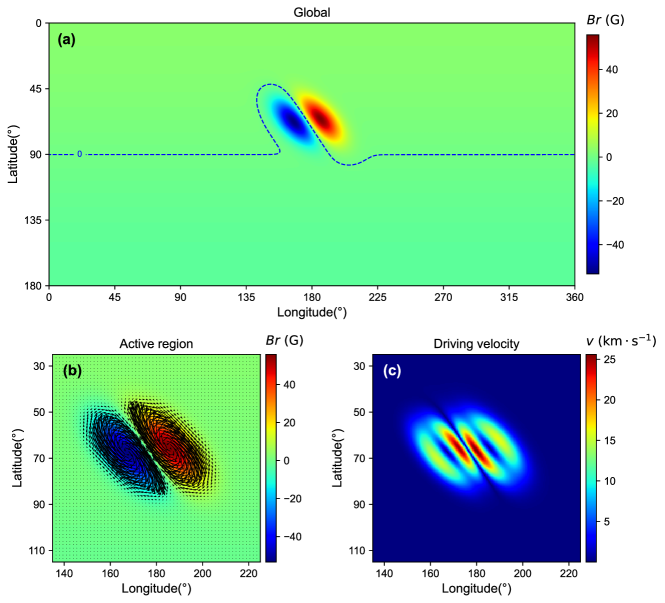
Figure 1: Map of magnetic flux density on the solar surface. (a) The global map. The PIL is shown by the dashed curve. (b) The active region; the arrows show the surface driving flow. (c) The driving velocity.

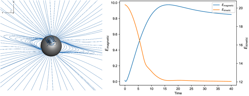
Figure 2: Simulation of the steady-state solar wind. In the left panel, the sphere shows the solar surface with contour of magnetic flux density $B_{r}$. The lines are magnetic field lines. The right panel shows temporal evolution of the magnetic and kinetic energies in the relaxation process.

2 Numerical Model

2.1 The control equations

We numerically solve the 3D MHD equations in 3D using the AMR–CESE–MHD code (Jiang et al., 2010). The MHD equations are given as

$$\frac{\partial\rho}{\partial t}+\nabla\cdot(\rho{\mathbf{v}})=0,$$

$$\rho\frac{D{\mathbf{v}}}{Dt}=-{\mathbf{\nabla}p+{\mathbf{J}}\times{\mathbf{B}}}+\rho{\mathbf{g}}+\nabla\cdot(\nu\rho\nabla{\mathbf{v}}),$$

$$\frac{\partial{\mathbf{B}}}{\partial t}=\nabla\times({\mathbf{v}\times{\mathbf{B}}}),$$

$$\frac{\partial T}{\partial t}+\nabla\cdot(T{\mathbf{v}})=(2-\gamma)T\nabla\cdot{\mathbf{v}}.$$ (1)

Here ${\mathbf{v}}$ represents the velocity, ${\mathbf{J}=\nabla\times{\mathbf{B}}}/\mu_{0}$ (with $\mu_{0}$ denotes the magnetic permeability in a vacuum) is the current density, ${\mathbf{g}}$ refers to the gravitational acceleration exerted by the Sun, $T$ is the temperature, and $\gamma$ is the adiabatic index, which is given as $\gamma=1.05$ to approximate a near-isothermal process.

In the code, all the variables are normalized by typical values in the corona. The values are, respectively, $L_{s}=6.96\times 10^{2}$ Mm (i.e., solar radius) for length, $\rho_{s}=1.67\times 10^{-15}$ g cm^-3 for density, $T_{s}=10^{6}$ K for temperature, $p_{s}=\rho_{s}RT_{s}$ (where $R$ is the gas constant) for pressure, $v_{s}=\sqrt{p_{s}/\rho_{s}}=1.28\times 10^{2}$ km s^-1 for velocity, $B_{s}=\sqrt{\mu_{0}p_{s}}=1.86$ G for magnetic field, $t_{s}=L_{s}/v_{s}=5.42\times 10^{3}$ s for time, and $E_{s}=\rho_{s}v_{s}^{2}L_{s}^{3}=9.31\times 10^{31}$ erg for energy.

In the magnetic induction equation, the trigger of the magnetic reconnection depends on the specific choice of magnetic diffusivity $\eta$. To avoid this sensitivity issue, we use no explicit form of $\eta$ in the magnetic induction equation, following Jiang et al. (2021). This approach minimizes resistivity and maximizes the Lundquist number at given spatial resolutions, as any non-zero $\eta$ would lead to greater resistivity than the numerical resistivity alone. Consequently, magnetic reconnection occurs only when the current layer becomes sufficiently narrow, approaching the grid resolution, where numerical diffusivity becomes significant.

2.2 Grid settings

The computational domain is a spherical shell ranging from the solar surface to around $20$ solar radii, where the solar wind becomes already supersonic and super-Alfvénic. The lower boundary is set at the solar surface, and more exactly, the base of the corona, while the upper boundary is positioned far enough to study the near-Sun propagation of a CME. We used a Yin-Yang grid to avoid the polar problems (i.e., grid singularity) of the standard spherical grid (Jiang et al., 2012). The Yin-Yang grid is composed by two low latitude partial-sphere grids, identical but with different orientations, to cover the full sphere with small patches overlapped (see Figure 1 of Jiang et al. (2012)). The computation utilizes block-structured adaptive mesh refinement (AMR), which dynamically adjusts grid resolution based on the evolving features during the simulation to improve accuracy and efficiency. For this study, the base resolution in latitude ($\Delta\theta$) and longitude ($\Delta\phi$) is set to $2^{\circ}$, and the AMR is configured to achieve a maximum refinement level of $4$. Therefore, the highest resolution is $0.25^{\circ}$. The grid cells are configured to be close to regular cubes by setting $\Delta r=r\Delta\theta$ (therefore not uniform in radial direction), and the highest resolution near the solar surface is $\Delta r\approx 4\times 10^{-3}$. We pay particular attention to the formation and reconnection of the current sheet in the simulation. The formation and evolution of current sheet are tracked by refining regions with both $J/B>4.0$ and plasma beta $\beta<0.25$ to the highest level. Additionally, areas where $|\nabla(B^{2}/2)|\Delta/\rho>15$ and $|(B\cdot\nabla)B|\Delta/\rho>15$ (where $\Delta$ is the grid resolution) are also refined to ensure high resolution in regions with strong magnetic field gradients and curvatures.

2.3 Initial conditions

The simulation is initialized with a plasma specified by the Parker’s classic spherically symmetrical model of solar wind and a potential (i.e., current free) magnetic field. The Parker model is solved by assuming an ideal adiabatic gas with $\gamma=1.05$, and constrained by a solar surface density $\rho=\rho_{s}$ and temperature $T=1.8~T_{s}$. The magnetic field comprises a background dipole field to represent the global coronal magnetic structure during solar minimum and an embedded small bipolar field representing an active region. We first specify the magnetogram, i.e., a map of the radial magnetic field component $B_{r}$ on the solar surface, and then compute the corresponding potential field for the whole simulation volume, using a fast solver (Jiang & Feng, 2012). The map is given by $B_{r}=B_{r}^{\rm g}+B_{r}^{\rm a}$, with $B_{r}^{\rm g}$ for the global field and $B_{r}^{\rm a}$ for the active region. The global component $B_{r}^{\rm g}$ is assumed to the solar surface flux of a dipole ${\mathbf{B}}_{\rm d}$ with magnetic moment ${\mathbf{m}}=(0,0,1.5)$ placed at the solar center,

$${\mathbf{B}}_{\rm d}=\frac{3({\mathbf{m}}\cdot{\mathbf{r}}){\mathbf{r}}}{r^{5}}-\frac{{\mathbf{m}}}{r^{3}}.$$ (2)

The active region component is given by the sum of two 2D Gaussian functions on the $(\theta,\phi)$ plane,

$$B_{r}^{\rm a}= B_{0}e^{-\frac{\theta^{\prime 2}}{\sigma_{\theta}^{2}}}e^{-\frac{(\varphi^{\prime}-\varphi_{\text{offset}})^{2}}{\sigma_{\varphi}^{2}}}-$$

$$B_{0}e^{-\frac{(\theta^{\prime}+\theta_{\text{slip}})^{2}}{\sigma_{\theta}^{2}}}e^{-\frac{(\varphi^{\prime}+\varphi_{\text{offset}})^{2}}{\sigma_{\varphi}^{2}}}.$$ (3)

Here $(\theta^{\prime},\phi^{\prime})$ are rotated coordinates with respect to the original coordinates $(\theta,\phi)$ given by

$$\begin{pmatrix}\varphi^{\prime}\\ \theta^{\prime}\end{pmatrix}=\begin{pmatrix}\cos\alpha&-\sin\alpha\\ \sin\alpha&\cos\alpha\end{pmatrix}\begin{pmatrix}\varphi-\phi_{0}\ \\ \theta-\theta_{0}\end{pmatrix}$$ (4)

where $(\theta_{0},\phi_{0})$ is the center of the active region, and $\alpha$ the rotation angle. By rotating the coordinate system, it is convenient to mimic active regions with different orientations. $\sigma_{\theta}$ and $\sigma_{\phi}$ control the extent of the magnetic flux distribution in the $\theta^{\prime}$ and $\phi^{\prime}$ directions, respectively, and $\phi_{\rm offset}$ controls the separation of the two polarities. Here the parameters are given as $B_{0}=48$ G, $\theta_{0}=70^{\circ}$, $\sigma_{\theta}=9^{\circ}$, $\phi_{0}=180^{\circ}$, $\sigma_{\phi}=9^{\circ}$, $\phi_{\rm offset}=6^{\circ}$, and $\alpha=45^{\circ}$. We further used a parameter $\theta_{\rm slip}=10^{\circ}$ to form a shearing shape between the positive and negative polarities along the polarity inversion line (PIL). Figure 1 shows the $B_{r}$ map. As can be seen, the field configuration resembles a typical bipolar solar active region located in the northern hemisphere during it’s decaying phase, and sheared by the differential rotation of the Sun.

2.4 Boundary conditions

Our simulation consists of different stages featured by specifying different velocity at the inner boundary (i.e., the solar surface). One is a relaxation stage, i.e., no external driver is applied, in which the surface velocity is simply given as $v_{r}=v_{\theta}=v_{\phi}=0$. The other is a driving stage in which the surface velocity is given as a surface rotation flow at each polarity of the AR to inject free magnetic energy into the AR. Following Jiang et al. (2021), the driving flow is incompressible with streamlines aligning with the contour lines of $B_{r}$, therefore not altering the profile of $B_{r}$ on the surface. Specifically, the surface velocity is set as

$$v_{r}=0,v_{\theta}=\frac{1}{R\sin\theta}\frac{\partial\Psi(B_{r})}{\partial\phi},v_{\phi}=-\frac{1}{R}\frac{\partial\Psi(B_{r})}{\partial\theta}$$ (5)

with $\Psi$ given by

$$\Psi=kB_{r}^{2}e^{-(B_{r}^{2}-B_{r,\mathrm{max}}^{2})/B_{r,\mathrm{max}}^{2}}$$ (6)

where $B_{r,\mathrm{max}}$ is the maximum value of $B_{r}$ at the surface, and $k$ is a scaling constant chosen so that the maximum surface velocity is $25.6$ km s^-1. The flow pattern is depicted in Figure 1. We note that this velocity is about an order of magnitude higher than typical photospheric motion speeds, which are approximately a few km s^-1 (Amari et al., 1996; Tokman & Bellan, 2002; Török & Kliem, 2003; DeVore & Antiochos, 2008). We intend to accelerate the surface driving to compete the effects of numerical dissipation of the accumulated free energy in the simulation, such that enough free energy can be stored in the simulated active region to produce an eruption. In Jiang et al. (2021)’s simulation they used a very high resolution to reduce the numerical diffusion and thus they were able to apply a rather slow driving speed of a few km s^-1 that is close to the actual photospheric motion. However, for a global simulation in this paper, it is expensive to use a high resolution to reduce the numerical diffusion, and therefore we choose to enlarge the driving speed.

We fix the plasma density and temperature at the bottom surface to its initial uniform value since the surface flow is incompressible. With the velocity prescribed (either as zero or by Equation 5) and $B_{r}$ unchanged, only the evolution of the horizontal magnetic field needs to be solved, by using the magnetic induction equation,

$$\frac{\partial{\mathbf{B}}}{\partial t}=-\nabla\times{\mathbf{E}}$$ (7)

The equation is discretized using a 2nd-order difference in space and a forward difference scheme in time. Specifically, we first compute the electric field at the grid points by assuming that ${\mathbf{E}}=-{\mathbf{v}}\times{\mathbf{B}}$, and then using a central different in $\theta$ and $\phi$ directions and a one-sided 2nd-order difference in $r$ direction. Taking the $B_{\theta}$ component as an example, the induction equation is casted in spherical coordinates as

$$\frac{\partial B_{\theta}}{\partial t}=\frac{1}{r\sin\theta}\frac{\partial(-E_{r})}{\partial\phi}-\frac{1}{r}\frac{\partial(-rE_{\phi})}{\partial r},$$ (8)

for which the numerical scheme is given by

$$\frac{(B_{\theta})_{i,j,0}^{n+1}-(B_{\theta})_{i,j,0}^{n}}{\Delta t}=\frac{(-E_{r})_{i,j+1,0}^{n+1/2}-(-E_{r})_{i,j-1,0}^{n+1/2}}{2r_{0}\sin{\theta_{i}}\Delta\phi}-$$

$$\frac{(\Delta r_{1}+\Delta r_{0})^{2}\Gamma_{1}-\Delta r_{0}^{2}\Gamma_{2}-\Delta r_{1}(\Delta r_{1}+2\Delta r_{0})\Gamma_{0}}{r_{0}\Delta r_{0}\Delta r_{1}(\Delta r_{0}+\Delta r_{1})}$$ (9)

where $\Gamma_{k}=r_{k}(-E_{\phi})_{i,j,k}$, the subscripts $i$, $j$, $k$ represent the grid points in the $\theta$, $\phi$, $r$ directions respectively, with $k=0$ corresponding to the points at the bottom boundary (note that no ghost layer is used in our code), and $\Delta r_{k}=r_{k+1}-r_{k}$. This approach allows for a self-consistently update of the magnetic field and facilitates simulation of the line-tied effect at the bottom boundary, which is crucial for the success of this simulation. For the outer boundary, we implemented non-reflecting conditions for all variables using the projected-characteristic method (see details in, e.g., Hayashi, 2005; Wu et al., 2006; Jiang et al., 2011; Feng et al., 2012).

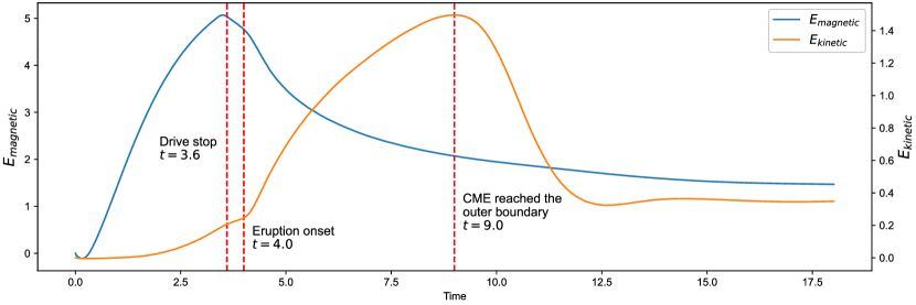
Figure 3: Evolution of magnetic energy (blue line) and kinetic energy (orange line) in the driving and eruption phases. The vertical dashed lines from left to right denote respectively the stopping time of surface driving, the eruption onset time, and the time when the leading edge of CME starts to leave the simulation volume.

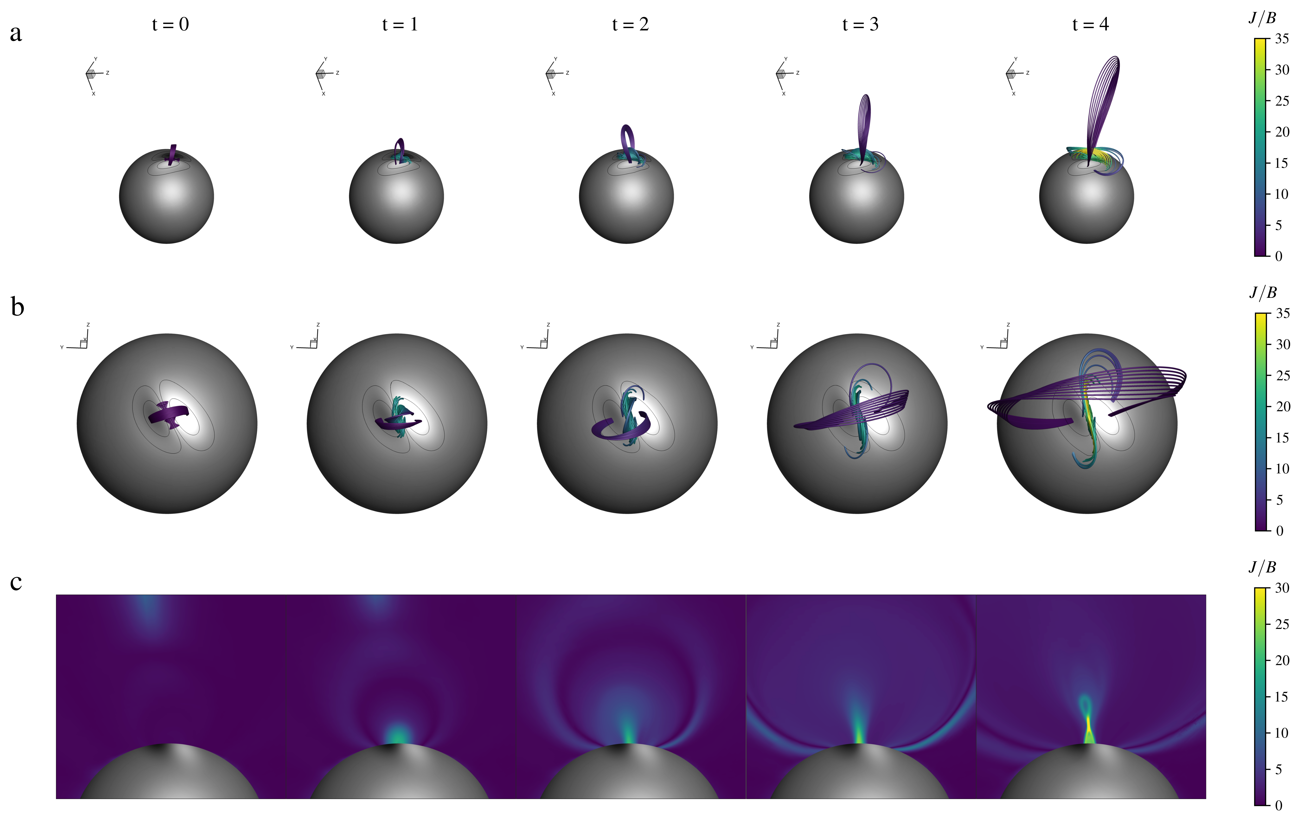
Figure 4: Evolution of magnetic field lines and electric currents prior to eruption. (a) Top view of magnetic field lines at different times in the simulation. The colored thick lines represent magnetic field lines, with colors denoting the value of the current density normalized by magnetic field strength ($J/B$). (b) 3D prospective view of the same field lines shown in panel a. (c) Vertical cross-section of $J/B$.

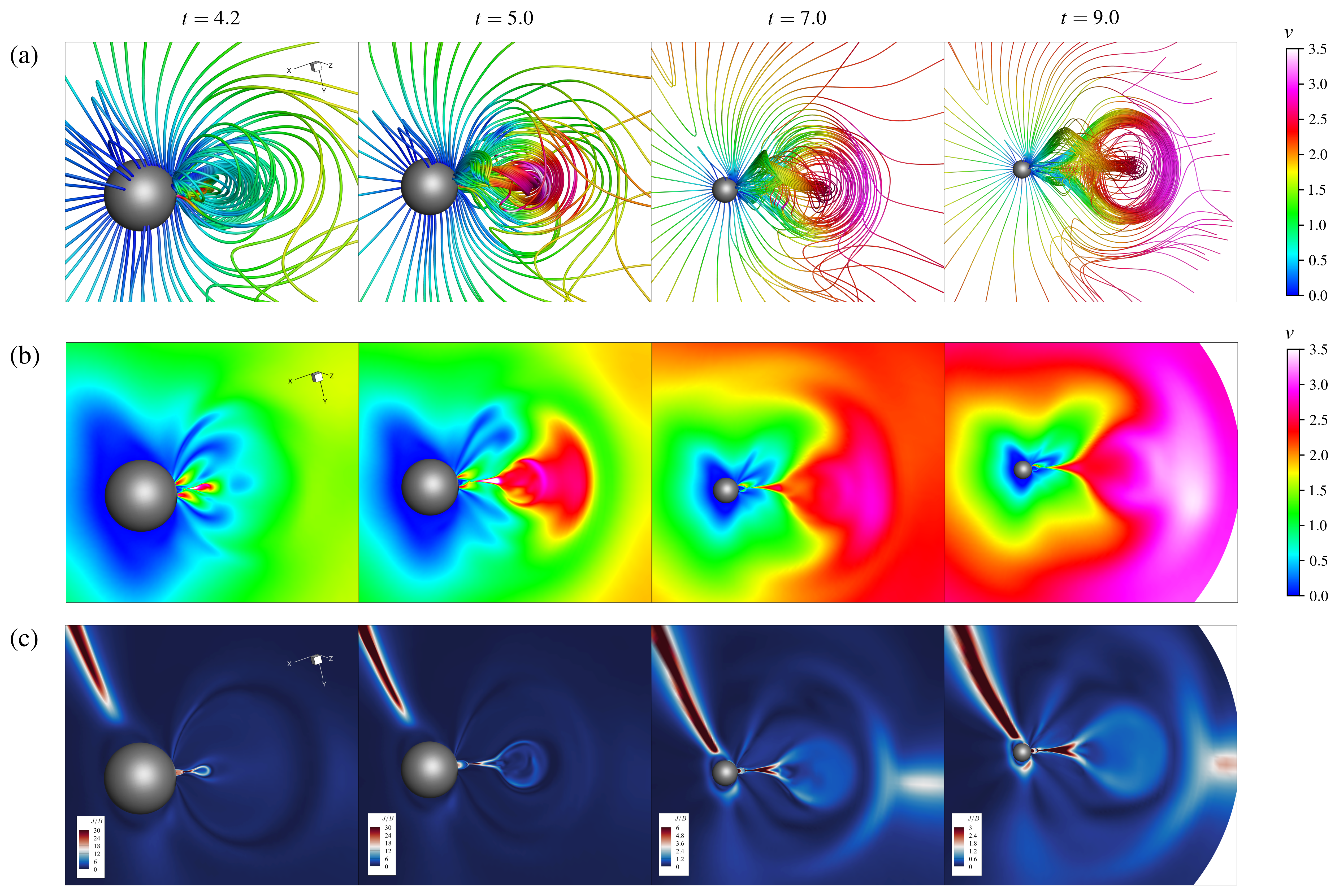
Figure 5: Evolution of magnetic field lines (a), velocity (b) and current density (c) of the CME. In all the panels, the gray sphere represents the surface of the Sun, and different fields of view are shown for different times. The magnetic field lines are pseudo-colored by velocity. The current density is shown normalized by the magnetic field strength (i.e., $J/B$). The velocity and current density are shown on the same cross section of the volume.

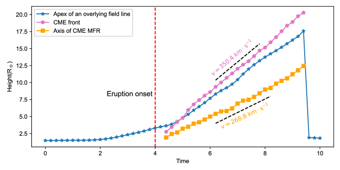
Figure 6: Variation of heights of the apex of an overlying magnetic field line of the active region’s sheared core, the CME front and the axis of the CME MFR. The velocity of the structures is shown by the dashed lines with numbers.

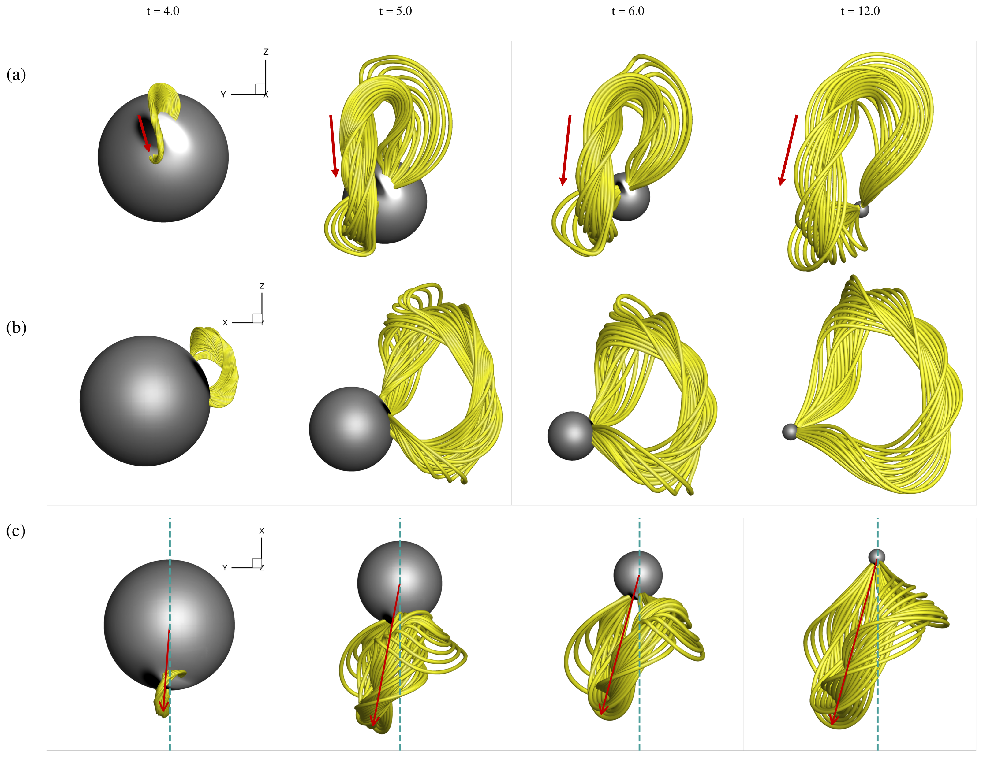
Figure 7: Evolution of the CME MFR at four different times (from left to right). Three view angles are shown from top to bottom. The sphere represents the solar surface shown with magnetic flux distribution. The thick lines show the magnetic field lines traced close to the axis of the MFR. In (a), the arrows show the direction of the axis of the MFR of CME at different times. In (c) the arrows the propagation direction of the MFR.

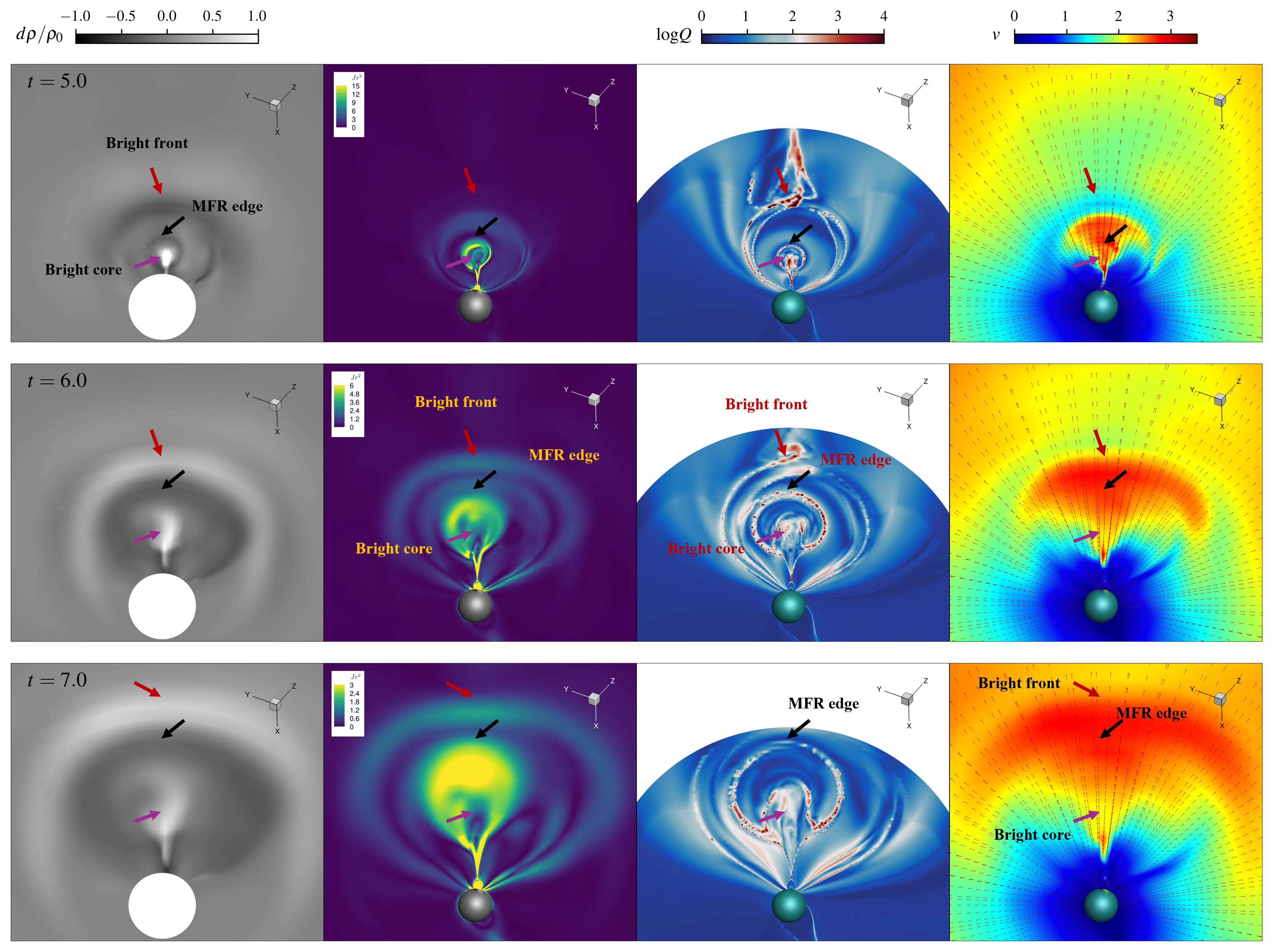
Figure 8: Cross section profiles of the density (the first column), current density (the second column), magnetic squashing factor (the third column) and the velocity (the last column) at three different times (from top to bottom). All panels show the same cross section of the volume with strictly the same view angle and field of view. For density, the ratio is defined as $d\rho/\rho_{0}=[\rho(t)-\rho(0)]/\rho(0)$, and the area within 2 solar radii is blanked to mimic the occulter of coronagraph. For current density, a factor of $r^{2}$ is multiplied. The squashing factor is computed only up to 12 solar radii. For the velocity, the thin arrows show the direction of the flow. In all the panels, the three thick arrows, from top to bottom, denote respectively the location of the bright front, the edge of the MFR, and the bright core. Not that for comparison, the location of each arrow in the same time is identical in the four different panels.

3 Results

We first perform a relaxation process (i.e., no surface driving flow) to achieve a steady-state solar wind solution, which provides a background for the subsequent simulation of CME triggering and evolution. Figure 2 shows the relaxed magnetic field lines and the evolution of energies during the relaxation process. As driven by the solar wind, the magnetic field lines from the two poles become eventually open, while at the low latitudes forms the helmet-like coronal streamer. With opening of the field lines, the magnetic energy is increased at the price of the kinetic energy loss. The relaxation process is stopped at $t=40$, when both the two energies become almost unchanged (albeit that the magnetic energy shows slow decrease due to the numerical resistivity). Once this relaxed state is established, we then introduce the rotational velocity to the active region to simulate photospheric motion that injects free magnetic energy into the system.

Figure 3 shows the energy evolution, and the time is reset with $t=0$ for the start of applying the surface driving flow. Note that the background values are subtracted from the energies, and therefore at $t=0$ both the energies are zero. As can be seen, with the driving flow applied, the magnetic energy keeps increasing. The kinetic energy also increased but is much slower. This indicates that the AR system evolves mostly quasi-statically. Since the driving speed is much higher than the real photospheric speed, to avoid a too much twisting of the field lines, we turn off the surface driving at $t=3.6$, shortly before the eruption onset time of $t=4.0$. At $t=4.0$, i.e., onset of the eruption, the kinetic energy shows a rapid increase and the magnetic energy shows a rapid decrease. This transition corresponds to fast release of the free magnetic energy, which drives an impulsive acceleration of the plasma.

Figures 4 and 5 illustrate the evolution of magnetic field lines and current density structures before and during the eruption. The evolution is almost identical to that of Jiang et al. (2021)’s simulation in a local Cartesian coordinates. The pre-eruption stage is featured by a slow shearing and expansion of the active region field within which a current sheet is gradually formed above the PIL. Due to the maximum gradient of velocity along the PIL, strong shear develops in the magnetic field lines at that location, forming an S-shaped structure. This S-shape is essentially composed of two sets of J-shaped magnetic field lines, which are created as the magnetic field in the active region is sheared in opposite directions by the rotational flow. Initially, the current is distributed volumetrically, but it is subsequently compressed into a vertical, narrow layer extending above the PIL, i.e., the current sheet (Figure 4c).

The eruption is triggered once magnetic reconnection starts in the current sheet. An MFR originates from the tip of the current sheet and quickly ascends, leaving behind a cusp-shaped structure that separates the post-flare loops from the un-reconnected magnetic field regions (Figure 5). As driven by the ongoing reconnection, the MFR rapidly grows, forming a CME. Figure 6 shows the time-height profile of the CME, including the leading edge of the CME and the apex of the MFR axis. As can be seen, the leading edge of the CME shows a radial velocity of approximately $350$ km s^-1, and the rope axis has a velocity of $270$ km s^-1. In addition, we traced the motion of the field line with footpoint fixed at the center of the positive polarity of the AR. This field line can correspond to a coronal loop in observation, initially located in the core of the active region. The coronal loop rises slowly from $t=2$ to around $4.5$, resembling the slow-rise phase in observed initiation process of many CMEs (Zhang & Dere, 2006; Cheng et al., 2020). The kinetic energy gained by the plasma, primarily in the CME, accounts for approximately one-third of the released magnetic energy (Figure 4). This suggests that the remaining two-thirds of the energy is consumed by the flare, which aligns with the typical energy partitioning between flares and CMEs in eruptive events (Emslie et al., 2012). At around $t=9$, the leading edge of CME reaches the outer boundary, and with the leaving of the CME from the computational volume, the kinetic energy decreases and is eventually restored to its pre-eruption value.

Figure 7 shows the evolution of the MFR, for which sampled magnetic field lines near the axis are plotted. Besides the growth (due to reconnection) and expansion, the MFR experiences a noticeable rotation that is often observed in the early phase of CME evolution (Manchester et al., 2017). At the very beginning of the eruption, the MFR axis directs mainly along the PIL of the AR (see the panels for $t=4$) since the MFR is formed from reconnection of the highly sheared arcade. Subsequently, the MFR rotates clockwise into a mainly southward direction. If direct to the Earth, this simulated CME could render a strong geomagnetic effect as it has a southward magnetic field component. The direction of rotation is consistent with the findings in Zhou et al. (2020) that during its eruption an forward (reverse) S-shaped MFR, as manifested by eruptive filament, rotates clockwise (anti-clockwise), and can be explained by the interaction of the erupting MFR with the background field (Zhou et al., 2023). The MFR is also deflected to the east, although slightly, during its propagation, which can be seen in the bottom panels of Figure 7. It is known that the deflection of CME can be attributed to the interaction of CME with the solar wind (Wang et al., 2004), e.g., a CME faster (slower) than the ambient solar wind would be deflected to the east (west). Our simulation supports this, as here the CME has a speed larger than that of the ambient solar wind during the simulated time interval (see Figure 5). The deflection of CME is also an important factor in determining the geomagnetic effect by changing the propagation path.

Figure 8 (left column) shows the density profile on a central cross section of the CME. The cross section is roughly perpendicular to axis of the MFR. We used the ratio $d\rho/\rho_{0}=[\rho(t)-\rho(0)]/\rho(0)$ to highlight the variation of the density relative to its background value. As can be seen, the density profile presents a three-part structure, namely a bright core, a dark cavity and a bright front, which resembles typical coronagraph observations. To understand the relationship between the three parts and the corresponding magnetic configuration, we plot the distribution of current density in the second column of Figure 8. Due to the fast expansion of the MFR, the current density is multiplied by a factor of $r^{2}$ to more clearly show the entire structure of the MFR. For more precisely locating the interface between the MFR and the overlying field, we also computed the magnetic squashing factor (Titov & Démoulin, 1999; Démoulin, 2006), from which the quasi-separatrix layer corresponding to the boundary of the MFR can be identified. Compared in the right column of Figure 8 is the distribution of velocity on the cross section, which is useful to analyze how the different structures of the density is formed. Since there is no filament in our simulation, the bright core does not correspond to a filament. By comparing the density profile and the current distribution, we can see that the bright core is located mainly at the lower part of the erupting MFR. Furthermore, the formation of the bright core can be understood from structure of the velocity; the fast reconnection outflow, driven by the strong slingshot effect (i.e., the outward magnetic tension force) of the newly-reconnected field lines, injects continuously plasma into the MFR, and this plasma is piled up at the lower part of the MFR because the fast reconnection jet is decelerated briefly after merging into the MFR (see also Jiang et al., 2021). As a result, the density becomes high there, forming the bright core. The dark cavity initially corresponds to the weakly sheared field overlying the highly-sheared core. During subsequent evolution, this field gradually reconnects and joins into the MFR as its envelope part, and thus part of the dark cavity now corresponds to this envelope part of the MFR. The low density in the cavity is a result of the fast expansion of the magnetic flux as it moves out and the ambient magnetic pressure decreases. Ahead of the dark cavity is the bright front, which is formed due to the compression of the plasma ahead of the CME’s high-speed region.

4 Conclusions

In this study, we presented a global-corona MHD simulation of the formation of a CME and its interaction with the ambient solar wind. We first constructed a background solar wind by relaxing the Parker’s solution with a global dipole field, which embeds a local bipolar field that represents an active region, to an MHD equilibrium. Then we energized the active region field using continuous shearing motion along the PIL until an eruption is produced. Our simulation encompassed the entire process from the gradual accumulation of magnetic energy to the catastrophic release of magnetic free energy that initiates the CME. The mechanism of CME initiation is in line with what has been shown in a previous simulation casted in local Cartesian coordinates (Jiang et al., 2021); an internal current sheet gradually forms within a sheared magnetic arcade and fast reconnection at this current sheet triggers and drives the eruption.

We further analyzed the subsequent evolution and propagation of the CME to around $0.1$ AU, highlighting key aspects such as the formation of MFR and its kinematic characteristics, deflection, rotation, and morphology, which may shed light on interpretation of observations. The MFR is originated and grows from the ongoing reconnection in the current sheet. Its axis reaches a speed of around $270$ km s^-1, while the CME front has a speed of $350$ km s^-1, somewhat faster than the simulated solar wind. As a forward S shaped MFR, it rotates clockwise during the evolution, and also exhibits a eastward deflection by interacting with the ambient solar wind. From the cross section profile of plasma density, the CME exhibits a typical three-part configuration. The bright core is mainly located at the lower part of the MFR and is produced by the plasma that is first rapidly ejected by the high-speed reconnection outflow and then piled up at the lower part of the MFR due to the brake down of the reconnection outflow. Therefore, a CME owning a bright core does not necessarily to contain a erupting filament, but with a filament, the core should be of course more prominent. The dark cavity contains both outer layer of the MFR and its overlying field (which is gradually integrated into the MFR due to the reconnection) that expands rapidly as the whole magnetic structure moves out. The bright front is formed due to the compression of the plasma ahead of the fast-moving magnetic structure.

We note that our model is still far from a realistic description of CME initiation and evolution. Future developments are needed, for example, by constructing a more realistic background solar wind with empirical coronal heating and acceleration that can produce a two-mode (i.e., fast and slow) wind structure (Feng et al., 2011); the observed synoptic magnetograms should be used to construct the global coronal magnetic field such that the CME can be initiated in a realistic magnetic environment (Mikić et al., 2018; Török et al., 2018); furthermore, the data-driven technique based on vector magnetograms should be used to follow the evolution and eruption of real active regions (Jiang et al., 2022). With these improvements, a in-depth understanding of the birth, 3D structure and evolution of CME is hopeful to achieve, and the model can be incorporated into Sun-to-Earth space weather modelling framework.

Data Availability

All the data generated for this paper are available from the authors upon request.

References

- Amari et al. (1996) Amari T., Luciani JF., Aly JJ., Tagger M., 1996, ASTROPHYSICAL JOURNAL, 466, L39+
- Amari et al. (2003) Amari T., Luciani JF., Aly JJ., Mikic Z., Linker J., 2003, ASTROPHYSICAL JOURNAL, 585, 1073
- Antiochos et al. (1999) Antiochos S. K., DeVore C. R., Klimchuk J. A., 1999, The Astrophysical Journal, 510, 485
- Aulanier (2013) Aulanier G., 2013, Proceedings of the International Astronomical Union, 8, 184
- Aulanier et al. (2010) Aulanier G., Toeroek T., Demoulin P., DeLuca E. E., 2010, ASTROPHYSICAL JOURNAL, 708, 314
- Bothmer & Schwenn (1998) Bothmer V., Schwenn R., 1998, ANNALES GEOPHYSICAE-ATMOSPHERES HYDROSPHERES AND SPACE SCIENCES, 16, 1
- Chen (2011) Chen P. F., 2011, Living Reviews in Solar Physics, 8, 1
- Chen (2017) Chen J., 2017, Physics of Plasmas, 24, 090501
- Chen & Shibata (2000) Chen P. F., Shibata K., 2000, The Astrophysical Journal, 545, 524
- Cheng et al. (2014) Cheng X., et al., 2014, ASTROPHYSICAL JOURNAL, 780
- Cheng et al. (2020) Cheng X., Zhang J., Kliem B., Torok T., Xing C., Zhou Z. J., Inhester B., Ding M. D., 2020, ASTROPHYSICAL JOURNAL, 894
- DeVore & Antiochos (2008) DeVore C. R., Antiochos S. K., 2008, ASTROPHYSICAL JOURNAL, 680, 740
- Démoulin (2006) Démoulin P., 2006, Advances in Space Research, 37, 1269
- Emslie et al. (2012) Emslie A. G., et al., 2012, The Astrophysical Journal, 759, 71
- Feng et al. (2011) Feng X., Zhang S., Xiang C., Yang L., Jiang C., Wu S. T., 2011, The Astrophysical Journal, 734, 50
- Feng et al. (2012) Feng X., Jiang C., Xiang C., Zhao X., Wu S. T., 2012, The Astrophysical Journal, 758, 62
- Forbes (2000) Forbes TG., 2000, JOURNAL OF GEOPHYSICAL RESEARCH-SPACE PHYSICS, 105, 23153
- Forbes et al. (2006) Forbes T. G., et al., 2006, Space Science Reviews, 123, 251
- Gopalswamy (2004) Gopalswamy N., 2004, in Poletto G., Suess S. T., eds, , Vol. 317, The Sun and the Heliosphere as an Integrated System. Springer Netherlands, Dordrecht, pp 201–251, doi:10.1007/978-1-4020-2831-1_8
- Gosling et al. (1976) Gosling J. T., Hildner E., MacQueen R. M., Munro R. H., Poland A. I., Ross C. L., 1976, Solar Physics, 48, 389
- Groth et al. (2000) Groth C. P. T., De Zeeuw D. L., Gombosi T. I., Powell K. G., 2000, Journal of Geophysical Research: Space Physics, 105, 25053
- Guo et al. (2024) Guo J. H., et al., 2024, Astronomy & Astrophysics, 690, A189
- Hayashi (2005) Hayashi K., 2005, The Astrophysical Journal Supplement Series, 161, 480
- Howard & DeForest (2012) Howard T. A., DeForest C. E., 2012, ASTROPHYSICAL JOURNAL, 746
- Howard & Pizzo (2016) Howard T. A., Pizzo V. J., 2016, ASTROPHYSICAL JOURNAL, 824
- Illing & Hundhausen (1985) Illing R. M. E., Hundhausen A. J., 1985, Journal of Geophysical Research: Space Physics, 90, 275
- Jiang (2024) Jiang C., 2024, Science China Earth Sciences, 67, 3765
- Jiang & Feng (2012) Jiang C., Feng X., 2012, Solar Physics, 281, 621
- Jiang et al. (2010) Jiang C., Feng X., Zhang J., Zhong D., 2010, SOLAR PHYSICS, 267, 463
- Jiang et al. (2011) Jiang C., Feng X., Fan Y., Xiang C., 2011, The Astrophysical Journal, 727, 101
- Jiang et al. (2012) Jiang C., Feng X., Xiang C., 2012, The Astrophysical Journal, 755, 62
- Jiang et al. (2021) Jiang C., et al., 2021, Nature Astronomy, 5, 1126
- Jiang et al. (2022) Jiang C., Feng X., Guo Y., Hu Q., 2022, The Innovation, 3, 100236
- Jin et al. (2017) Jin M., et al., 2017, The Astrophysical Journal, 834, 173
- Joselyn & McIntosh (1981) Joselyn J. A., McIntosh P. S., 1981, Journal of Geophysical Research: Space Physics, 86, 4555
- Kataoka et al. (2009) Kataoka R., Ebisuzaki T., Kusano K., Shiota D., Inoue S., Yamamoto T. T., Tokumaru M., 2009, Journal of Geophysical Research: Space Physics, 114, n/a
- Kleimann (2012) Kleimann J., 2012, Solar Physics
- Koehn et al. (2022) Koehn G. J., Desai R. T., Davies E. E., Forsyth R. J., Eastwood J. P., Poedts S., 2022, The Astrophysical Journal, 941, 139
- Kumar & Innes (2013) Kumar P., Innes D. E., 2013, SOLAR PHYSICS, 288, 255
- Kusano et al. (2012) Kusano K., Bamba Y., Yamamoto T. T., Iida Y., Toriumi S., Asai A., 2012, The Astrophysical Journal, 760, 31
- Lepri & Zurbuchen (2010) Lepri S. T., Zurbuchen T. H., 2010, ASTROPHYSICAL JOURNAL LETTERS, 723, L22
- Linan et al. (2024) Linan L., Baratashvili T., Lani A., Schmieder B., Brchnelova M., Guo J., Poedts S., 2024, Astronomy & Astrophysics
- Lionello et al. (2013) Lionello R., Downs C., Linker J. A., Török T., Riley P., Mikić Z., 2013, The Astrophysical Journal, 777, 76
- Lugaz et al. (2011) Lugaz N., Downs C., Shibata K., Roussev I. I., Asai A., Gombosi T. I., 2011, The Astrophysical Journal, 738, 127
- Lugaz et al. (2023) Lugaz N., et al., 2023, Bulletin of the AAS
- Luhmann et al. (2020) Luhmann J. G., Gopalswamy N., Jian L. K., Lugaz N., 2020, Solar Physics, 295, 61
- Manchester (2004) Manchester W. B., 2004, Journal of Geophysical Research, 109, A01102
- Manchester et al. (2017) Manchester W., Kilpua E. K. J., Liu Y. D., Lugaz N., Riley P., Török T., Vršnak B., 2017, Space Science Reviews, 212, 1159
- Mei et al. (2023) Mei Z., Ye J., Li Y., Xu S., Chen Y., Hu J., 2023, The Astrophysical Journal, 958, 15
- Mikic & Linker (1994) Mikic Z., Linker J. A., 1994, The Astrophysical Journal, 430, 898
- Mikić et al. (2018) Mikić Z., et al., 2018, Nature Astronomy, 2, 913
- Riley et al. (2006) Riley P., Linker J., Mikic Z., Odstrcil D., 2006, Advances in Space Research, 38, 535
- Schmieder et al. (2015) Schmieder B., Aulanier G., Vršnak B., 2015, Solar Physics, 290, 3457
- Shen et al. (2016) Shen F., Wang Y., Shen C., Feng X., 2016, Scientific Reports, 6, 19576
- Song et al. (2017) Song H. Q., et al., 2017, The Astrophysical Journal, 848, 21
- Song et al. (2023) Song H., Li L., Zhou Z., Xia L., Cheng X., Chen Y., 2023, The Astrophysical Journal Letters, 952, L22
- Song et al. (2025) Song H., Li L., Wang B., Xia L., Chen Y., 2025, The Astrophysical Journal, 978, 40
- Temmer et al. (2023) Temmer M., et al., 2023, Advances in Space Research, p. S0273117723005239
- Titov & Démoulin (1999) Titov V. S., Démoulin P., 1999, Astronomy & Astrophysics, 351, 707
- Tokman & Bellan (2002) Tokman M., Bellan PM., 2002, ASTROPHYSICAL JOURNAL, 567, 1202
- Török & Kliem (2003) Török T., Kliem B., 2003, ASTRONOMY & ASTROPHYSICS, 406, 1043
- Török & Kliem (2005) Török T., Kliem B., 2005, The Astrophysical Journal, 630, L97
- Török et al. (2018) Török T., et al., 2018, The Astrophysical Journal, 856, 75
- Török et al. (2023) Török T., et al., 2023, Bulletin of the AAS
- Van der Holst et al. (2005) Van der Holst B., Poedts S., Chané E., Jacobs C., Dubey G., Kimpe D., 2005, Space Science Reviews, 121, 91
- Wang et al. (2004) Wang Y., Shen C., Wang S., Ye P., 2004, Solar Physics, 222, 329
- Webb & Howard (2012) Webb D. F., Howard T. A., 2012, Living Reviews in Solar Physics, 9
- Wood et al. (2016) Wood B. E., Howard R. A., Linton M. G., 2016, ASTROPHYSICAL JOURNAL, 816
- Wu et al. (2006) Wu S. T., Wang A. H., Liu Y., Hoeksema J. T., 2006, The Astrophysical Journal, 652, 800
- Yang et al. (2021) Yang L., et al., 2021, The Astrophysical Journal, 918, 31
- Zhang & Dere (2006) Zhang J., Dere K. P., 2006, ASTROPHYSICAL JOURNAL, 649, 1100
- Zhang et al. (2021) Zhang J., et al., 2021, Progress in Earth and Planetary Science, 8, 56
- Zhou et al. (2014) Zhou Y., Feng X., Zhao X., 2014, Journal of Geophysical Research: Space Physics, 119, 9321
- Zhou et al. (2020) Zhou Z., Liu R., Cheng X., Jiang C., Wang Y., Liu L., Cui J., 2020, The Astrophysical Journal, 891, 180
- Zhou et al. (2023) Zhou Z., Jiang C., Yu X., Wang Y., Hao Y., Cui J., 2023, Frontiers in Physics, 11, 1119637