Convergence analysis of decoupled mixed FEM for the Cahn-Hilliard-Navier-Stokes equations

Abstract

We develop a decoupled, first-order, fully discrete, energy-stable scheme for the Cahn-Hilliard-Navier-Stokes equations. This scheme calculates the Cahn-Hilliard and Navier-Stokes equations separately, thus effectively decoupling the entire system. To further separate the velocity and pressure components in the Navier-Stokes equations, we use the pressure-correction projection method. We demonstrate that the scheme is primitively energy stable and prove the optimal $L^{2}$ error estimate of the fully discrete scheme in the $P_{r}\times P_{r}\times P_{r}\times P_{r-1}$ finite element spaces, where the phase field, chemical potential, velocity and pressure satisfy the first-order accuracy in time and the $\left(r+1,r+1,r+1,r\right)th$-order accuracy in space, respectively. Furthermore, numerical experiments are conducted to support these theoretical findings. Notably, compared to other numerical schemes, our algorithm is more time-efficient and numerically shown to be unconditionally stable.

Keywords: Phase field models; Cahn-Hilliard-Navier-Stokes; convex-splitting; energy stability; optimal error estimates.

1 Introduction

The Cahn-Hilliard-Navier-Stokes (CHNS) model features a nonlinear interaction between the incompressible Navier-Stokes (NS) equations [1] and the Cahn-Hilliard (CH) equations [2]. This model captures the interfacial dynamics of two-phase, incompressible, and macroscopically immiscible Newtonian fluids that exhibit matched densities [3, 4] as follows:

$$\frac{\partial\phi}{\partial t}+(\mathbf{u}\cdot\nabla)\phi-M\Delta\mu=0,\quad\text{in}\quad\Omega\times(0,T],$$ (1.1a)

$$\mu+\lambda\Delta\phi-\lambda F^{\prime}(\phi)=0,\quad\text{in}\quad\Omega\times(0,T],$$ (1.1b)

$$\frac{\partial\mathbf{u}}{\partial t}+(\mathbf{u}\cdot\nabla)\mathbf{u}-\nu\Delta\mathbf{u}+\nabla p-\mu\nabla\phi=0,\quad\text{in}\quad\Omega\times(0,T],$$ (1.1c)

$$\nabla\cdot\mathbf{u}=0,\quad\text{in}\quad\Omega\times(0,T],$$ (1.1d)

with the following boundary and initial conditions of (1.1):

$$\frac{\partial\phi}{\partial\mathbf{n}}=\frac{\partial\mu}{\partial\mathbf{n}}=0,\quad\mathbf{u}=0, \quad\text{on}\quad\partial\Omega\times(0,T],$$ (1.2a)

$$\phi(\mathbf{x},0)=\phi^{0},\quad\mathbf{u}(\mathbf{x},0)=\mathbf{u}^{0}, \quad\text{in}\quad\Omega.$$ (1.2b)

Here $\Omega\subset\mathbb{R}^{d},~(d=2,3)$ is a bounded convex polygonal or polyhedral domain, and for $t\in(0,T]$, and $F(\phi)=\frac{1}{4\epsilon^{2}}\left(\phi^{2}-1\right)^{2}$. In the model, $\phi$ represents the phase field variable, and $\mu$ denotes the chemical potential, and the $\mathbf{u}$ and $p$ are the velocity and pressure of the fluid, respectively. $\epsilon$ is the interfacial width between the two phases field, and the parameters $M$, $\lambda$ and $\nu$ represent the mobility constant, the mixing coefficient and the fluid viscosity, respectively. It is well know that the energy of CHNS model is defined by

$$E(\phi,\mathbf{u})=\int_{\Omega}\left(\frac{1}{2}|\mathbf{u}|^{2}+\frac{\lambda}{2}|\nabla\phi|^{2}+\lambda F(\phi)\right)dx.$$ (1.3)

The system (1.1)-(1.2) satisfies the following energy dissipation law at $\forall t\in(0,T]$,

$$\frac{\partial E(\phi(t),\mathbf{u}(t))}{\partial t}=-M\|\nabla\mu\|^{2}-\nu\|\nabla\mathbf{u}\|^{2}.$$ (1.4)

Over the past decade or so, one of the primary challenges for the CH equations have been the efficient treatment of nonlinear terms to ensure that the resulting discretized system is solved efficiently while maintaining energy stability. Some of the techniques for dealing with the nonlinear terms in the numerical format of the CH equation include the convex splitting [5], stabilized semi-implicit methods [6], invariant energy quadratization (IEQ) [7], and the scalar auxiliary variable (SAV) approach [8, 9]. On the other hand, the main challenges in solving the NS equations lie in the treatment of nonlinear terms and the coupling between velocity and pressure under incompressible conditions. For the coupling between velocity and pressure, a widely adopted strategy is the projection method [10], originally proposed by Chorin and Temam [11]. The nonlinear terms in the NS equations can be handled either in an fully implicit, semi-implicit, or through SAV full explicatization. Wang et al. [12] presented a novel second order in time mixed finite element scheme for the Cahn–Hilliard–Navier–Stokes equations with matched densities, and they [13] proposed and analyze a time second-order accurate numerical scheme for the Cahn–Hilliard-Magnetohydrodynamics equations. As a result, based on the several challenges mentioned earlier, a large number of scholars have worked on proposing energy-stable and efficient numerical schemes for CHNS [14, 15, 16, 17, 18, 19, 20, 21, 22, 12, 23].

Recently, Xu et al. [20] proposed a first-order in time, linear, fully decoupled, and energy stable scheme for the CHNS model. They introduced a velocity intermediate quantity in the discretization of the CH equation, thus explicitly dealing with the coupling term between the velocity and phase functions. The introduction of this intermediate variable makes error estimation involved, especially if one also wants to obtain optimal $L^{2}$ error estimates for the spatial variables. Then, Wen et al. [24] proposed a novel fully discrete stabilized finite element method using the lowest equal-order finite elements, and they analyzed the optimal $H^{1}$ error estimates for the phase field function, chemical potential and velocity. Cai et al. [25] first presented optimal $L^{2}$ error estimates of the convex splitting finite element method for the CHNS system. However, these schemes are a coupled system, whose numerical results in relatively long computation time. Soon after, Yang et al. [26] proposed a step-by-step decoupling method that utilizes the SAV approach to split the CHNS model into CH and NS components, enabling the solution of these two equations separately, and also analyzed the optimal $L^{2}$ error estimates for the numerical solution, but their scheme did not achieve original energy stabilization.

To the best of our knowledge, there is no literature on the optimal $L^{2}$ error estimates for the fully decoupled, original energy stable numerical scheme of CHNS model. To achieve this purpose, we firstly decouple the CH and NS equations by handling the convective term implicitly/explicitly in the CH equation, thus resulting in a fully decoupled and original energy stable semi-discrete scheme. Secondly, we discretize the spatial variables using the mixed finite element method to obtain a fully decoupled, fully discretized scheme with original energy stable, which is analyzed to obtain the optimal $L^{2}$ error estimate. We notice that Kay et al. [4] also constructed a fully decoupled numerical scheme with original energy stabilization, they, however, did not provide the optimal $L^{2}$ error estimates. Additionally, Cai et al. [25] analytically derived the optimal $L^{2}$ error estimates for the scheme with original energy stabilization, but the coupled nature of their scheme made computation expensive. We emphasize that despite a mild time-step restriction is imposed in our energy stability, our numerical experiment demonstrates that our fully decoupled scheme is unconditionally energy stable.

This manuscript is organized as follows: The Section 2 introduces fundamental notations and lemmas. In Section 3, we propose a fully decoupled, energy-stable scheme utilizing fully discrete mixed finite element methods based on pressure-correction and convex splitting techniques for the CHNS model; we then prove the energy stability of our scheme. In Section 4, we provide the corresponding error estimates and establish optimal $L^{2}$ error estimates for the fully discrete scheme. Numerical experiments are conducted in Section 5 to validate the theoretical results of our scheme.

2 The mathematical prelimilaries

In the section, we introduce some mathematical notations. For any integer $k\geq 0$ and $1\leq p\leq\infty$, let $W^{k,p}(\Omega)$ be the Sobolev space, we denote $H^{k}(\Omega)=W^{k,2}(\Omega)$ and $L^{p}(\Omega)=W^{0,p}(\Omega)$. The norm of $L^{2}$ denote by $\|\cdot\|$ and the closure of $C_{0}^{\infty}(\Omega)$ in $W^{k,p}$ space denotes by $W_{0}^{k,p}$ and $H_{0}^{k}(\Omega)=W_{0}^{k,p}$. Let $\mathbf{L}^{p}(\Omega)=[L^{p}(\Omega)]^{d}$, $\mathbf{H}_{0}^{1}(\Omega)=[H_{0}^{1}(\Omega)]^{d}$, $\mathbf{W}^{k,p}(\Omega)=[W^{k,p}(\Omega)]^{d}$ the corresponding vector valued Sobolev spaces with the norms $\|\cdot\|_{H^{k}}$ and $\|\cdot\|_{L^{p}}$. For $\bm{v}\in\mathbf{H}^{1}(\Omega)$ and $\phi,~w\in H^{1}(\Omega)$, we define the trilinear form $b(\cdot,\cdot,\cdot)$ by

$$b(\phi,\bm{v},w)=\left(\nabla\phi\cdot\bm{v},w\right),$$ (2.1)

and for $\bm{u},\bm{v},\bm{w}\in\mathbf{H}^{1}(\Omega)$, we define the trilinear form $\bm{B}(\cdot,\cdot,\cdot)$ by

$$\bm{B}(\bm{u},\bm{v},\bm{w})=\frac{1}{2}\left(\left(\bm{u}\cdot\nabla\right)\bm{v},\bm{w}\right)-\frac{1}{2}\left((\bm{u}\cdot\nabla)\bm{w},\bm{v}\right).$$ (2.2)

It is well-know result that

$$\bigg{|}b(\phi,\bm{v},w)\bigg{|}=\bigg{|}\int_{\Omega}w\nabla\phi\cdot\bm{v}dx\bigg{|}\leq\|\phi\bm{v}\|\|\nabla w\|\leq\|\phi\|_{L^{4}}\|\bm{v}\|_{L^{4}}\|\nabla w\|\leq\|\phi\|_{H^{1}}\|\bm{v}\|_{H^{1}}\|\nabla w\|.$$ (2.3)

We next introduce the Ritz and Stokes projections. Let $\mathcal{T}_{h}$ denotes a quasi-uniform partition of $\Omega$ into triangles $\mathcal{K}_{j},~j=1,\cdots,M$, in $\mathbb{R}^{2}$ with mesh size $h=\max_{1\leq j\leq M}\{\dim\mathcal{K}_{j}\}$. For a given positive integer $r\geq 2$, we set the phase field-velocity-pressure finite element spaces

$$S_{h}^{r}=\left\{v_{h}\in C(\Omega):\left.v_{h}\right|_{\mathcal{K}_{j}}\in P_{r}\left(\mathcal{K}_{j}\right),\forall\mathcal{K}_{j}\in\mathcal{T}_{h}\right\},$$ (2.4)

$$\mathring{S}_{h}^{r-1}=S_{h}^{r-1}\cap L_{0}^{2}(\Omega),$$

$$\mathbf{X}_{h}^{r}=\left\{\mathbf{v}_{h}\in\mathbf{H}_{0}^{1}(\Omega)^{d}:\left.\mathbf{v}_{h}\right|_{\mathcal{K}_{j}}\in\mathbf{P}_{r}\left(\mathcal{K}_{j}\right)^{d},\forall\mathcal{K}_{j}\in\mathcal{T}_{h}\right\},$$

where $P_{r}\left(\mathcal{K}_{j}\right)$ is the space of polynomials of degree $r$ on $\mathcal{K}_{j}$. For some constant $C>0$, it is well-known that both the Taylor-Hood elements satisfy the discrete inf-sup condition [27]

$$\left\|q_{h}\right\|_{L^{2}}\leq C\sup_{\mathbf{0}\neq\mathbf{v}_{h}\in\mathbf{X}_{h}^{r}}\frac{\left(q_{h},\nabla\cdot\mathbf{v}_{h}\right)}{\left\|\nabla\mathbf{v}_{h}\right\|},\quad\forall q_{h}\in\mathring{S}_{h}^{r-1}.$$ (2.5)

For the simplicity of notations and $r\geq 2$, we define

$$\mathbf{\mathcal{X}}_{h}^{r}=S_{h}^{r}\times S_{h}^{r}\times\mathbf{X}_{h}^{r}\times\mathring{S}_{h}^{r-1},$$ (2.6)

and denote $\bm{g}^{n+1}=\bm{g}\left(x,t^{n+1}\right)$, and

$$\delta_{\tau}\bm{g}^{n+1}=\frac{\bm{g}^{n+1}-\bm{g}^{n}}{\tau}.$$ (2.7)

Remark 2.1.

In an abuse of notation, we use $\bm{g}^{n+1}$ hereafter to denote the value of the exact solution $\bm{g}$ at $t^{n+1}$.

We will frequently use the following discrete version of the Grönwall lemma [28]:

Lemma 2.1 (discrete Grönwall inequality [28]).

For all $0\leq n\leq m$, let $a_{n},b_{n},c_{n},d_{n},\tau,C\geq 0$ such that

$$a_{m}+\tau\sum_{n=0}^{m}b_{n}\leq\tau\sum_{n=0}^{m}d_{n}a_{n}+\tau\sum_{n=0}^{m}c_{n}+C,$$ (2.8)

suppose that $\tau d_{n}<1$, for all $n\geq 0$, and set $\sigma_{n}=(1-\tau d_{n})^{-1}$. Then

$$a_{m}+\tau\sum_{n=0}^{m}b_{n}\leq\exp\left(\tau\sum_{n=0}^{m}\sigma_{n}d_{n}\right)\left\{a_{0}+\left(b_{0}+c_{0}\right)\tau+\tau\sum_{n=1}^{m}c_{n}\right\}.$$ (2.9)

Throughout the manuscript we use $C$ or $c$, with or without subscript, to denote a positive constant independent of discretization parameters that could have uncertain values in different places.

3 The numerical scheme

In the section, we construct first-order fully decoupled scheme, and prove that the numerical scheme satisfies energy stabilization. For $r\geq 2$, we assume that the solutions to the CHNS model (1.1) in this manuscript exist and satisfy the following regularity assumption:

$$\phi\in L^{\infty}\left(0,T;H^{r+1}(\Omega)\right),~\phi_{t}\in L^{\infty}\left(0,T;H^{1}(\Omega)\right)\cap L^{2}\left(0,T;H^{1}(\Omega)\right),\phi_{tt}\in L^{2}\left(0,T;L^{2}(\Omega)\right),$$ (3.1)

$$\mu\in L^{\infty}\left(0,T;H^{r+1}(\Omega)\right),~\mu_{t}\in L^{\infty}\left(0,T;H^{1}(\Omega)\right),~p\in L^{\infty}\left(0,T;H^{r}(\Omega)\right),~p_{t}\in L^{2}\left(0,T;H^{r}(\Omega)\right),$$

$$\mathbf{u}\in L^{\infty}\left(0,T;\mathbf{H}^{r+1}(\Omega)\right),~\mathbf{u}_{t}\in L^{\infty}\left(0,T;\mathbf{H}^{1}(\Omega)\right)\cap L^{2}\left(0,T;\mathbf{H}^{r+1}(\Omega)\right),~\mathbf{u}_{tt}\in L^{2}\left(0,T;\mathbf{H}^{-1}(\Omega)\right).$$

3.1 Fully discrete scheme

In the subsection, we construct a decoupled, first-order and fully discrete finite elements method based on Euler implicit-explict scheme for solving the CHNS system. For any test functions $w\in H^{1}(\Omega)$, $\varphi\in H^{1}(\Omega)$, $\mathbf{v}\in\mathbf{H}_{0}^{1}(\Omega)$, $q\in L_{0}^{2}(\Omega)$, the weak solutions $\left(\phi,\mu,\mathbf{u},p\right)$ of (1.1) satisfy the following variational forms:

$$\left(\partial_{t}\phi,w\right)+M\left(\nabla\mu,\nabla w\right)+b\left(\phi,\mathbf{u},w\right) =0,$$ (3.2)

$$\left(\mu,\varphi\right)-\lambda\left(\nabla\phi,\nabla\varphi\right)-\frac{\lambda}{\epsilon^{2}}\left(\phi^{3}-\phi,\varphi\right) =0,$$ (3.3)

$$\left(\partial_{t}\mathbf{u},\mathbf{v}\right)+\nu\left(\nabla\mathbf{u},\nabla\mathbf{v}\right)+\bm{B}\left(\mathbf{u},\mathbf{u},\mathbf{v}\right)+\left(\nabla p,\mathbf{v}\right)-b\left(\phi,\mathbf{v},\mu\right) =0,$$ (3.4)

$$\left(\nabla\cdot\mathbf{u},q\right) =0.$$ (3.5)

Let $N$ be a positive integer and $\left\{t^{n}=n\tau\right\}_{n=0}^{N}$ denotes a uniform partition of the time interval $[0,T]$ with a step size $\tau=T/N$. For $n\geq 0$, choosing the initial conditions $\left(\phi_{h}^{0},\mu_{h}^{0},\mathbf{u}_{h}^{0},p_{h}^{0}\right)$ and $\left(\phi_{h}^{n},\mu_{h}^{n},\mathbf{u}_{h}^{n},p_{h}^{n}\right)$, and updating $\left(\phi_{h}^{n+1},\mu_{h}^{n+1},\tilde{\mathbf{u}}_{h}^{n+1},\mathbf{u}_{h}^{n+1},p_{h}^{n+1}\right)$, we construct the following fully decoupled, energy stable scheme for the CHNS system.
$\mathbf{Step1.}$ Find $\left(\phi_{h}^{n+1},\mu_{h}^{n+1}\right)\in\left(S_{h}^{r},S_{h}^{r}\right)$ such that

$$\left(\delta_{\tau}\phi_{h}^{n+1},w_{h}\right)+b\left(\phi_{h}^{n+1},\mathbf{u}_{h}^{n},w_{h}\right)+M\left(\nabla\mu_{h}^{n+1},\nabla w_{h}\right)=0,$$ (3.6)

$$\left(\mu_{h}^{n+1},\varphi_{h}\right)-\lambda\left(\nabla\phi_{h}^{n+1},\nabla\varphi_{h}\right)-\frac{\lambda}{\epsilon^{2}}\left(\left(\phi_{h}^{n+1}\right)^{3}-\phi_{h}^{n},\varphi_{h}\right)=0,$$ (3.7)

$$\partial_{n}\phi_{h}^{n+1}|_{\partial\Omega}=0,~\partial_{n}\mu_{h}^{n+1}|_{\partial\Omega}=0.$$ (3.8)

$\mathbf{Step2.}$ Find $\tilde{\mathbf{u}}_{h}^{n+1}\in\mathbf{X}_{h}^{r}$ such that

$$\left(\frac{\tilde{\mathbf{u}}_{h}^{n+1}-\mathbf{u}_{h}^{n}}{\tau},\mathbf{v}_{h}\right)+\bm{B}\left(\mathbf{u}_{h}^{n},\tilde{\mathbf{u}}_{h}^{n+1},\mathbf{v}_{h}\right)+\nu\left(\nabla\tilde{\mathbf{u}}_{h}^{n+1},\nabla\mathbf{v}_{h}\right)+\left(\nabla p_{h}^{n},\mathbf{v}_{h}\right)-b\left(\phi_{h}^{n+1},\mathbf{v}_{h},\mu_{h}^{n+1}\right)=0,$$ (3.9)

$$\tilde{\mathbf{u}}_{h}^{n+1}|_{\partial\Omega}=0.$$ (3.10)

$\mathbf{Step3.}$ Find $\left(p_{h}^{n+1},\mathbf{u}_{h}^{n+1}\right)\in\left(\mathring{S}_{h}^{r-1},\mathbf{X}_{h}^{r}\right)$ such that

$$\frac{\mathbf{u}_{h}^{n+1}-\tilde{\mathbf{u}}_{h}^{n+1}}{\tau}+\nabla\left(p_{h}^{n+1}-p_{h}^{n}\right)=0,$$ (3.11)

$$\left(\nabla\cdot\mathbf{u}_{h}^{n+1},q_{h}\right)=0,~\mathbf{u}_{h}^{n+1}\cdot\mathbf{n}|_{\partial\Omega}=0,$$ (3.12)

hold for all $\left(w_{h},\varphi_{h},\mathbf{v}_{h},q_{h}\right)\in\mathbf{\mathcal{X}}_{h}^{r}$, and $n=0,1,2,\cdots,N-1$, where $\phi_{h}^{0}=R_{h}\phi^{0},~\mathbf{u}_{h}^{0}=\mathbf{I}_{h}\mathbf{u}^{0}.$ For simplicity of description, we perform the fully discretization to prove that our numerical scheme satisfies energy stabilization. For the convenience of the following theoretical analysis, we set the parameters $\lambda,M,\nu$ to 1.

3.2 Energy stability

For the above scheme, we can establish the theorem of energy stabilization as follows:

Theorem 3.1.

Let $\phi_{h}^{n}\in S_{h}^{r}$ and $\mathbf{u}_{h}^{n}\in\mathbf{X}_{h}^{r}$ and the initial values $|\phi_{h}^{0}|\leq C_{1}$ and $E(\phi_{h}^{0},\mathbf{u}_{h}^{0})\leq C_{0}$, i.e., the initial energy is bounded. For all time partitions $\tau$ and mesh size $h$ such that $\tau\leq\min\{Ch/\left(2\|\phi_{h}^{n}\|_{L^{4}}^{2}\right)\}$, the decoupled scheme (3.6)-(3.12) is uniquely solvable and satisfies discrete energy law as follows:

$$\tilde{E}_{h}^{n+1}-\tilde{E}_{h}^{n}\leq-M\tau\|\nabla\mu_{h}^{n+1}\|^{2}-2\nu\tau\|\nabla\tilde{\mathbf{u}}_{h}^{n+1}\|^{2},$$ (3.13)

where $\tilde{E}_{h}^{n+1}$ is defined by

$$\tilde{E}_{h}^{n+1}=\lambda\|\nabla\phi_{h}^{n+1}\|^{2}+\frac{\lambda}{2\epsilon^{2}}\|(\phi_{h}^{n+1})^{2}-1\|^{2}+\|\mathbf{u}_{h}^{n+1}\|^{2}+\tau^{2}\|\nabla p_{h}^{n+1}\|^{2},$$ (3.14)

and $C_{0}$ and $C_{1}$ are constant that does depend on the initial value of $\phi$ and $\mathbf{u}$.

Proof.

Letting $w_{h}=2\tau\mu_{h}^{n+1}$ in (3.6), we can obtain

$$2\left(\phi_{h}^{n+1}-\phi_{h}^{n},\mu_{h}^{n+1}\right)+2\tau\left(\mathbf{u}_{h}^{n}\cdot\nabla\phi_{h}^{n+1},\mu_{h}^{n+1}\right)+2M\tau\|\nabla\mu_{h}^{n+1}\|^{2}=0.$$ (3.15)

Letting $\varphi_{h}=-2\left(\phi_{h}^{n+1}-\phi_{h}^{n}\right)$ in (3.7), we can obtain

$$-2\left(\mu_{h}^{n+1},\phi_{h}^{n+1}-\phi_{h}^{n}\right)+\lambda\left(\|\nabla\phi_{h}^{n+1}\|^{2}-\|\nabla\phi_{h}^{n}\|^{2}+\|\nabla\phi_{h}^{n+1}-\nabla\phi_{h}^{n}\|^{2}\right)$$ (3.16)

$$+\frac{2\lambda\tau}{\epsilon^{2}}\left(\frac{1}{4}\delta_{\tau}\|\left(\phi_{h}^{n+1}\right)^{2}-1\|^{2}+\frac{\tau}{4}\left(\|\delta_{\tau}(\phi_{h}^{n+1})^{2}\|^{2}+2\|\phi_{h}^{n+1}\delta_{\tau}\phi_{h}^{n+1}\|^{2}+2\|\delta_{\tau}\phi_{h}^{n+1}\|^{2}\right)\right) =0.$$

Letting $\mathbf{v}_{h}=2\tau\tilde{\mathbf{u}}_{h}^{n+1}$ in (3.9), we derive that

$$\|\tilde{\mathbf{u}}_{h}^{n+1}\|^{2}-\|\mathbf{u}_{h}^{n}\|^{2}+\|\tilde{\mathbf{u}}_{h}^{n+1}-\mathbf{u}_{h}^{n}\|^{2}+2\nu\tau\|\nabla\tilde{\mathbf{u}}_{h}^{n+1}\|^{2}+2\tau\left(\nabla p_{h}^{n},\tilde{\mathbf{u}}_{h}^{n+1}\right)-2\tau\left(\mu_{h}^{n+1}\nabla\phi_{h}^{n+1},\tilde{\mathbf{u}}_{h}^{n+1}\right)=0.$$ (3.17)

Next, we rewrite (3.11) as

$$\mathbf{u}_{h}^{n+1}+\tau\nabla p_{h}^{n+1}=\tilde{\mathbf{u}}_{h}^{n+1}+\tau\nabla p_{h}^{n}.$$ (3.18)

Then we derive from (3.18) that

$$\|\mathbf{u}_{h}^{n+1}\|^{2}-\|\tilde{\mathbf{u}}_{h}^{n+1}\|^{2}-2\tau\left(\nabla p_{h}^{n},\tilde{\mathbf{u}}_{h}^{n+1}\right)+\tau^{2}\left(\|\nabla p_{h}^{n+1}\|^{2}-\|\nabla p_{h}^{n}\|^{2}\right)=0.$$ (3.19)

Adding the (3.19) and (3.17), we can obtain

$$\|\mathbf{u}_{h}^{n+1}\|^{2} -\|\mathbf{u}_{h}^{n}\|^{2}+\|\tilde{\mathbf{u}}_{h}^{n+1}-\mathbf{u}_{h}^{n}\|^{2}+2\tau\|\nabla\tilde{\mathbf{u}}_{h}^{n+1}\|^{2}+\tau^{2}\left(\|\nabla p_{h}^{n+1}\|^{2}-\|\nabla p_{h}^{n}\|^{2}\right)$$ (3.20)

$$=2\tau\left(\mu_{h}^{n+1}\nabla\phi_{h}^{n+1},\tilde{\mathbf{u}}_{h}^{n+1}\right).$$

Combining the (3.15), (3.16) with (3.20), we get

$$\lambda\left(\|\nabla\phi_{h}^{n+1}\|^{2}\right. \left.-\|\nabla\phi_{h}^{n}\|^{2}+\|\nabla\phi_{h}^{n+1}-\nabla\phi_{h}^{n}\|^{2}\right)$$ (3.21)

$$+\frac{2\lambda\tau}{\epsilon^{2}}\left(\frac{1}{4}\delta_{\tau}\|\left(\phi_{h}^{n+1}\right)^{2}-1\|^{2}+\frac{\tau}{4}\left(\|\delta_{\tau}(\phi_{h}^{n+1})^{2}\|^{2}+2\|\phi_{h}^{n+1}\delta_{\tau}\phi_{h}^{n+1}\|^{2}+2\|\delta_{\tau}\phi_{h}^{n+1}\|^{2}\right)\right)$$

$$+\|\mathbf{u}_{h}^{n+1}\|^{2}-\|\mathbf{u}_{h}^{n}\|^{2}+\|\tilde{\mathbf{u}}_{h}^{n+1}-\mathbf{u}_{h}^{n}\|^{2}+\tau^{2}\left(\|\nabla p_{h}^{n+1}\|^{2}-\|\nabla p_{h}^{n}\|^{2}\right)$$

$$= -2M\tau\|\nabla\mu_{h}^{n+1}\|^{2}-2\nu\tau\|\nabla\tilde{\mathbf{u}}_{h}^{n+1}\|^{2}+2\tau\left(\mu_{h}^{n+1}\nabla\phi_{h}^{n+1},\tilde{\mathbf{u}}_{h}^{n+1}-\mathbf{u}_{h}^{n}\right).$$

Recalling inverse inequalities and choosing $\tau\leq Ch/\left(2\|\phi_{h}^{n}\|_{L^{4}}^{2}\right)$, we have

$$2\tau\bigg{|}\left(\mu_{h}^{n+1}\nabla\phi_{h}^{n+1},\tilde{\mathbf{u}}_{h}^{n+1}-\mathbf{u}_{h}^{n}\right)\bigg{|}\leq ~2\tau\|\phi_{h}^{n+1}\|_{L^{4}}\|\nabla\mu_{h}^{n+1}\|\|\tilde{\mathbf{u}}_{h}^{n+1}-\mathbf{u}_{h}^{n}\|_{L^{4}}$$ (3.22)

$$\leq ~C\tau\|\phi_{h}^{n+1}-\phi_{h}^{n}+\phi_{h}^{n}\|_{L^{4}}^{2}\|\tilde{\mathbf{u}}_{h}^{n+1}-\mathbf{u}_{h}^{n}\|_{L^{4}}^{2}+M\tau\|\nabla\mu_{h}^{n+1}\|^{2}$$

$$\leq ~\frac{1}{2}\|\nabla\phi_{h}^{n+1}-\nabla\phi_{h}^{n}\|^{2}+\frac{C_{2}\tau}{h}\|\phi_{h}^{n}\|_{L^{4}}^{2}\|\tilde{\mathbf{u}}_{h}^{n+1}-\mathbf{u}_{h}^{n}\|^{2}+M\tau\|\nabla\mu_{h}^{n+1}\|^{2},$$

where $C$ and $C_{2}$ are constant that does not depend on $\tau$ and $h$. Combining (3.22) with (3.21), and summing up form $n=0$ to $m$, we have

$$\tilde{E}_{h}^{m+1}-\tilde{E}_{h}^{0}\leq-\tau\sum_{n=0}^{m}\left(2\|\nabla\tilde{\mathbf{u}}_{h}^{n+1}\|^{2}+\|\nabla\mu_{h}^{n+1}\|^{2}\right)-\sum_{n=0}^{m}\left(1-\frac{C_{2}\tau}{h}\|\phi_{h}^{n}\|_{L^{4}}^{2}\right)\|\tilde{\mathbf{u}}_{h}^{n+1}-\mathbf{u}_{h}^{n}\|^{2}.$$ (3.23)

In order to the energy to satisfy the law of decay when $m=0$, the following conditions need to be satisfied

$$\tau\leq\frac{Ch}{\|\phi_{h}^{0}\|_{L^{4}}^{2}}.$$ (3.24)

Since $\|\phi_{h}^{0}\|_{L^{4}}\leq C\|\phi_{h}^{0}\|$ is bounded, the $\tau$ of the above equation (3.24) can be taken to a valid value such that

$$\tilde{E}_{h}^{1}-\tilde{E}_{h}^{0}\leq 0.$$ (3.25)

So we can obtain that $\|\phi_{h}^{1}\|$ is bounded. When $m=1$, we have

$$\tau\leq\min\bigg{\{}\frac{Ch}{\|\phi_{h}^{0}\|_{L^{4}}^{2}},\frac{Ch}{\|\phi_{h}^{1}\|_{L^{4}}^{2}}\bigg{\}},$$ (3.26)

then we can dervie that $\|\phi_{h}^{2}\|\leq C$. By analogy, we can obatin the following result

$$\tau\leq\min_{0\leq n\leq m}\bigg{\{}\frac{Ch}{\|\phi_{h}^{0}\|_{L^{4}}^{2}},~\frac{Ch}{\|\phi_{h}^{1}\|_{L^{4}}^{2}},~\cdots,~\frac{Ch}{\|\phi_{h}^{n}\|_{L^{4}}^{2}}\bigg{\}}.$$ (3.27)

Thus, we can always obtain a positive number $C$ such that $\|\phi_{h}^{n}\|_{L4}\leq C$ is bounded, and derive the desired result (3.13). ∎

Remark 3.1.

The existence of the solution for scheme (3.6)-(3.12) can be proved using the standard argument of the Leray-Schauder fixed point theorem (see [15, 4] for details of similar problems).

Then, we can derive the following lemma regarding the boundedness of the numerical solutions obtained from the scheme (3.6)-(3.12).

Lemma 3.1.

Let $\left(\phi_{h}^{n+1},\mu_{h}^{n+1},\tilde{\mathbf{u}}_{h}^{n+1},\mathbf{u}_{h}^{n+1},p_{h}^{n+1}\right)\in\mathbf{\mathcal{X}}_{h}^{r}$ be the unique solution of (3.6)-(3.12). Suppose that $E(\phi_{h}^{0},\mathbf{u}_{h}^{0})<C_{0}$, for any $h,\tau>0$ and $\tau\leq Ch/\left(2\|\phi_{h}^{n}\|_{L^{4}}^{2}\right)$, the following boundedness hold that

$$\max_{0\leq n\leq N-1}\left(\|\mathbf{u}_{h}^{n+1}\|^{2}+\|\nabla\phi_{h}^{n+1}\|^{2}+\frac{\tau}{2\epsilon^{2}}\|\left(\phi_{h}^{n+1}\right)^{2}-1\|^{2}+\tau^{2}\|\nabla p_{h}^{n+1}\|^{2}\right) \leq C_{0},$$ (3.28)

$$\tau\sum_{n=0}^{N-1}\left(\|\nabla\mu_{h}^{n+1}\|^{2}+\|\nabla\tilde{\mathbf{u}}_{h}^{n+1}\|^{2}\right) \leq C_{0},$$ (3.29)

$$\sum_{n=0}^{N-1}\left(\|\nabla\phi_{h}^{n+1}-\nabla\phi_{h}^{n}\|^{2}+\|\tilde{\mathbf{u}}_{h}^{n+1}-\mathbf{u}_{h}^{n}\|^{2}\right) \leq C_{0},$$ (3.30)

$$\frac{\tau^{2}}{\epsilon^{2}}\sum_{n=0}^{N-1}\left[\frac{1}{2}\|\delta_{\tau}(\phi_{h}^{n+1})^{2}\|^{2}+\|\phi_{h}^{n+1}\delta_{\tau}\phi_{h}^{n+1}\|^{2}+\|\delta_{\tau}\phi_{h}^{n+1}\|^{2}\right] \leq C_{0},$$ (3.31)

where $C_{0}$ is a positive constant dependent on the initial value of $\phi^{0}$ and $\mathbf{u}^{0}$.

The proof of this lemma can be derived from the result of Theorem 3.1, the detailed steps of which we omit.

Lemma 3.2.

For all $m\geq 0$, there exists positive constant $C$ such that

$$\|\phi_{h}^{m+1}\|_{H^{1}}^{2}+\tau\sum_{n=0}^{m}\|\mu_{h}^{n+1}\|^{2}\leq C\tau,$$ (3.32)

and

$$\|\Delta_{h}\phi_{h}^{m+1}\|^{2}+\tau\sum_{n=0}^{m}\|\Delta_{h}\mu_{h}^{n+1}\|^{2}\leq C\tau.$$ (3.33)

Proof.

Letting $w_{h}=2\tau\phi_{h}^{n+1}$ in (3.6), we obtain

$$\|\phi_{h}^{n+1}\|^{2}-\|\phi_{h}^{n}\|^{2}+\|\phi_{h}^{n+1}-\phi_{h}^{n}\|^{2}=-2\tau\left(\mathbf{u}_{h}^{n}\cdot\nabla\phi_{h}^{n+1},\phi_{h}^{n+1}\right)-2\tau\left(\nabla\mu_{h}^{n+1},\nabla\phi_{h}^{n+1}\right).$$ (3.34)

Using the Young inequality and Cauchy-Sachwarz inequality, we can obtain

$$\big{|}-2\tau\left(\mathbf{u}_{h}^{n}\cdot\nabla\phi_{h}^{n+1},\phi_{h}^{n+1}\right)\big{|}\leq ~2\tau\|\mathbf{u}_{h}^{n}\|_{L^{4}}\|\nabla\phi_{h}^{n+1}\|\|\phi_{h}^{n+1}\|_{L^{4}}$$ (3.35)

$$\leq ~\tau\|\nabla\phi_{h}^{n+1}\|^{2}+C\tau\|\nabla\mathbf{u}_{h}^{n}\|^{2}\left(\|\phi_{h}^{n+1}\|^{2}+\|\nabla\phi_{h}^{n+1}\|^{2}\right)$$

and

$$\big{|}-2\tau\left(\nabla\mu_{h}^{n+1},\nabla\phi_{h}^{n+1}\right)\big{|}\leq\tau\left(\|\nabla\mu_{h}^{n+1}\|^{2}+\|\nabla\phi_{h}^{n+1}\|^{2}\right).$$ (3.36)

Combining the above two inequalities with (3.34) and summing up for $n$ from $0$ to $m$, we obtain

$$\|\phi_{h}^{m+1}\|^{2}\leq\|\phi_{h}^{0}\|^{2}+\tau\sum_{n=0}^{m}\left(\|\nabla\mu_{h}^{n+1}\|^{2}+2\|\nabla\phi_{h}^{n+1}\|^{2}+C\|\nabla\mathbf{u}_{h}^{n}\|^{2}\left(\|\phi_{h}^{n+1}\|^{2}+\|\nabla\phi_{h}^{n+1}\|^{2}\right)\right).$$ (3.37)

Using the lemma 2.1 and 3.1, we have

$$\|\phi_{h}^{m+1}\|^{2}\leq\left(\|\phi_{h}^{0}\|^{2}+c_{1}\left(1+4\tau+c_{2}\right)\right)\exp(c)\leq C\tau.$$ (3.38)

Thererfore, we can derive

$$\|\phi_{h}^{n+1}\|_{H^{1}}^{2}\leq\|\phi_{h}^{n+1}\|^{2}+\|\nabla\phi_{h}^{n+1}\|^{2}\leq C\tau.$$ (3.39)

Testing $\varphi_{h}=\tau\mu_{h}^{n+1}$ in (3.7), we obtain

$$\tau\|\mu_{h}^{n+1}\|^{2}= ~\tau\left(\nabla\phi_{h}^{n+1},\nabla\mu_{h}^{n+1}\right)+\tau\left((\phi_{h}^{n+1})^{3}-\phi_{h}^{n},\mu_{h}^{n+1}\right)$$ (3.40)

$$\leq ~\tau\left(\|\nabla\phi_{h}^{n+1}\|^{2}+\|\nabla\mu_{h}^{n+1}\|^{2}+\|\mu_{h}^{n+1}\|^{2}+\|(\phi_{h}^{n+1})^{3}-\phi_{h}^{n}\|^{2}\right).$$

Now using the (2.37) in [29], we have

$$\|(\phi_{h}^{n+1})^{3}-\phi_{h}^{n}\|^{2}\leq 2\left(\|\phi_{h}^{n+1}\|_{L^{6}}^{6}+\|\phi_{h}^{n}\|^{2}\right)\leq C\left(\|\phi_{h}^{n+1}\|_{H^{1}}^{2}+\|\phi_{h}^{n}\|^{2}\right)\leq C.$$ (3.41)

Thus, combining the above inequalities with (3.40) and summing up for $n$ from $0$ to $m$, we obtain

$$\tau\sum_{n=0}^{m}\|\mu_{h}^{n+1}\|^{2}\leq C\tau.$$ (3.42)

From (3.39) and (3.42), we obtain the result of (3.32). We nextly prove the second term of this lemma. Letting $w_{h}=2\tau\Delta_{h}\mu_{h}^{n+1}$ in (3.6), and $\varphi_{h}=\Delta_{h}\delta_{\tau}\phi_{h}^{n+1}$ in (3.7), and combining the results of two terms, we obtain

$$~\|\Delta_{h}\phi_{h}^{n+1}\|^{2}-\|\Delta_{h}\phi_{h}^{n}\|^{2}+\|\Delta_{h}\left(\phi_{h}^{n+1}-\phi_{h}^{n}\right)\|^{2}+2\tau\|\Delta_{h}\mu_{h}^{n+1}\|^{2}$$ (3.43)

$$= ~2\tau\left(\mathbf{u}_{h}^{n}\cdot\nabla\phi_{h}^{n+1},\Delta_{h}\mu_{h}^{n+1}\right)+2\tau\left((\phi_{h}^{n+1})^{3}-\phi_{h}^{n},\Delta_{h}\delta_{\tau}\phi_{h}^{n+1}\right).$$

Using the Lemma 2.14 in [29], we can estimate the right-hand side of (3.43) as follows:

$$\big{|}2\tau\left(\mathbf{u}_{h}^{n}\cdot\nabla\phi_{h}^{n+1},\Delta_{h}\mu_{h}^{n+1}\right)\big{|}\leq ~2\tau\|\mathbf{u}_{h}^{n}\|_{L^{4}}^{2}\|\nabla\phi_{h}^{n+1}\|_{L^{4}}\|\Delta_{h}\mu_{h}^{n+1}\|$$ (3.44)

$$\leq ~C\tau\|\nabla\mathbf{u}_{h}^{n}\|\left(\|\nabla\phi_{h}^{n+1}\|+\|\Delta_{h}\phi_{h}^{n+1}\|\right)\|\Delta_{h}\mu_{h}^{n+1}\|$$

$$\leq ~C\tau\|\nabla\mathbf{u}_{h}^{n}\|^{2}\left(\|\nabla\phi_{h}^{n+1}\|^{2}+\|\Delta_{h}\phi_{h}^{n+1}\|^{2}\right)+\tau\|\Delta_{h}\mu_{h}^{n+1}\|^{2}.$$

and

$$\big{|}2\tau\left((\phi_{h}^{n+1})^{3}-\phi_{h}^{n},\Delta_{h}\delta_{\tau}\phi_{h}^{n+1}\right)\big{|}\leq ~2\tau\|(\phi_{h}^{n+1})^{3}-\phi_{h}^{n}\|\|\Delta_{h}\delta_{\tau}\phi_{h}^{n+1}\|$$ (3.45)

$$\leq ~c\tau^{2}\|\Delta_{h}\delta_{\tau}\phi_{h}^{n+1}\|^{2}+C.$$

Combining the above two inequalities (3.44) and (3.45) with (3.43) and summing up for $n$ from $0$ to $m$, we obtain

$$\|\Delta_{h}\phi_{h}^{m+1}\|^{2}+\tau\sum_{n=0}^{m}\|\Delta_{h}\mu_{h}^{n+1}\|^{2}\leq\|\Delta_{h}\phi_{h}^{0}\|^{2}+\tau\sum_{n=0}^{m}\|\nabla\mathbf{u}_{h}^{n}\|^{2}\left(\|\nabla\phi_{h}^{n+1}\|^{2}+\|\Delta_{h}\phi_{h}^{n+1}\|^{2}\right).$$ (3.46)

Using the lemma 2.1 and 3.1, we obtain the result of this lemma. ∎

Remark 3.2.

We note that the bound $\tau\leq Ch/\left(2\|\phi_{h}^{n}\|_{L^{4}}^{2}\right)$ in Lemma 3.1 and 3.2 is attainable, since from (4.26) and Lemma 3.2 we obtain $\|\phi_{h}^{n}\|_{L^{4}}\leq C\|\phi_{h}^{n}\|_{H^{1}}\leq C$. More similar details about energy stabilization under this discrete scheme can be found in reference [4].

4 Error analysis

In this section, we establish the error analysis for the scheme (3.6)-(3.12). Firstly, we denote $R_{h}:H^{1}(\Omega)\rightarrow S_{h}^{r}$ as the classic Ritz projection [30],

$$\left(\nabla\left(\psi-R_{h}\psi\right),\nabla\varphi_{h}\right)=0,\quad\forall~\psi\in H^{1}(\Omega),~\varphi_{h}\in S_{h}^{r}.$$ (4.1)

Now, for $s\in[2,\infty]$ and $n=1,2,\cdots,N$, from the finite element approximation theory [31], it holds that

$$\|\psi-R_{h}\psi\|_{L^{s}}+h\|\psi-R_{h}\psi\|_{W^{1,s}}\leq Ch^{r+1}\|\psi\|_{W^{r+1,s}},$$ (4.2)

$$\|\psi-R_{h}\psi\|_{H^{-1}}\leq Ch^{r+1}\|\psi\|_{H^{r+1}},$$ (4.3)

$$\|\delta_{\tau}\left(\psi^{n}-R_{h}\psi^{n}\right)\|+h\|\delta_{\tau}\left(\psi^{n}-R_{h}\psi^{n}\right)\|_{H^{1}}\leq Ch^{r+1}\|\delta_{\tau}\psi^{n}\|_{H^{r+1}},$$ (4.4)

$$\|\delta_{\tau}\left(\psi^{n}-R_{h}\psi^{n}\right)\|_{H^{-1}}\leq Ch^{r+1}\|\delta_{\tau}\psi^{n}\|_{H^{r+1}},$$ (4.5)

where $\delta_{\tau}$ is defined in (2.7). Let $I_{h}:L^{2}(\Omega)\rightarrow S_{h}^{r}$ and $\mathbf{I}_{h}:\mathbf{L}^{2}(\Omega)\rightarrow\mathbf{X}_{h}^{r}$ are defined the $L^{2}$ projection operators [32, 33] by

$$\left(v-I_{h}v,w_{h}\right)=0,~\forall w_{h}\in S_{h}^{r},$$ (4.6)

$$\left(\mathbf{v}-\mathbf{I}_{h}\mathbf{v},\mathbf{w}_{h}\right)=0,~\forall\mathbf{w}_{h}\in\mathbf{X}_{h}^{r}.$$ (4.7)

It is known to all that the $L^{2}$ projection satisfies the following estimates,

$$\left\|v-I_{h}v\right\|+h\left\|\nabla\left(v-I_{h}v\right)\right\|\leq Ch^{r+1}\|v\|_{H^{r+1}},$$ (4.8)

$$\left\|\mathbf{v}-\mathbf{I}_{h}\mathbf{v}\right\|+h\left\|\nabla\left(\mathbf{v}-\mathbf{I}_{h}\mathbf{v}\right)\right\|\leq Ch^{r+1}\|\mathbf{v}\|_{H^{r+1}}.$$ (4.9)

For $\left(\mathbf{v}_{h},q_{h}\right)\in\mathbf{X}_{h}^{r}\times\mathring{S}_{h}^{r-1}$, the Stokes projection [34] $P_{h}$ or $\mathbf{P}_{h}:\mathbf{H}_{0}^{1}(\Omega)\times L_{0}^{2}(\Omega)\rightarrow\mathbf{X}_{h}^{r}\times\mathring{S}_{h}^{r-1}$ are defined by

$$\left(\nabla\left(\mathbf{u}-\mathbf{P}_{h}(\mathbf{u},p)\right),\nabla\mathbf{v}_{h}\right)-\left(p-P_{h}(\mathbf{u},p),\nabla\cdot\mathbf{v}_{h}\right)=0,$$ (4.10)

$$\left(\nabla\cdot\left(\mathbf{u}-\mathbf{P}_{h}(\mathbf{u},p)\right),q_{h}\right)=0.$$ (4.11)

To be the simplicity of notations, we denote $P_{h}p=P_{h}(\mathbf{u},p)$ and $\mathbf{P}_{h}\mathbf{u}=\mathbf{P}_{h}(\mathbf{u},p)$.

Lemma 4.1 ([35, 25]).

Under the assumption of regularity (3.1), it holds that

$$\|\mathbf{u}-\mathbf{P}_{h}\mathbf{u}\|+h\left(\|\nabla\left(\mathbf{u}-\mathbf{P}_{h}\mathbf{u}\right)\|+\|p-P_{h}p\|\right)\leq Ch^{r+1}\left(\|\mathbf{u}\|_{H^{r+1}}+\|p\|_{H^{r}}\right),$$ (4.12)

and

$$\|\delta_{\tau}\left(\mathbf{u}^{n}-\mathbf{P}_{h}\mathbf{u}^{n}\right)\|\leq ~Ch^{r+1}\left(\|\delta_{\tau}\mathbf{u}^{n}\|_{H^{r+1}}+\|\delta_{\tau}p^{n}\|\right.$$ (4.13)

$$~\left.+\|\delta_{\tau}\phi^{n}\|_{H^{r+1}}\|\mu^{n}\|_{H^{2}}+\|\phi^{n-1}\|_{H^{r+1}}\|\delta_{\tau}\mu^{n}\|_{H^{2}}\right).$$

where $C$ is the constant the only depends on $\Omega$.

The proof of this lemma is similar to Lemma 3.2 of [25]. Here we omit the detailed procedure and refer the interested reader to [25].

Lemma 4.2 ([36]).

The Stokes projection $\mathbf{P}_{h}(\mathbf{u},p)$ is $\mathbf{H}^{1}$ stable in the case such that

$$\|\mathbf{P}_{h}(\mathbf{u},p)\|_{H^{1}}\leq C\left(\|\mathbf{u}\|_{H^{2}}+\|p\|_{H^{1}}\right).$$ (4.14)

Next we introduce the discrete Laplacian operator [37] $\Delta_{h}:\mathring{S}_{h}^{r-1}\rightarrow\mathring{S}_{h}^{r-1}$ such that

$$\left(-\Delta_{h}v_{h},\xi_{h}\right)=\left(\nabla v_{h},\nabla\xi_{h}\right),$$ (4.15)

$$\left(\nabla(-\Delta_{h}^{-1})v_{h},\nabla\xi_{h}\right)=\left(v_{h},\xi_{h}\right).$$ (4.16)

By defining the discrete Stokes operator $A_{h}=-\mathbf{I}_{h}\Delta_{h}$ [26], it holds

$$\|v_{h}\|_{H^{2}}=\|A_{h}v_{h}\|,~\|v_{h}\|_{H^{-1}}=\|A_{h}^{-1/2}v_{h}\|,~v_{h}\in\mathbf{X}_{h}^{r},$$ (4.17)

$$\|A_{h}^{1/2}v_{h}\|=\|\nabla v_{h}\|,~\|\nabla A_{h}^{-1/2}v_{h}\|=\|v_{h}\|,~v_{h}\in\mathbf{X}_{h}^{r}.$$ (4.18)

If $v_{h}$ is a constant, we denote $(-\Delta_{h})^{\frac{1}{2}}v_{h}=0$ and $(-\Delta_{h})^{-\frac{1}{2}}v_{h}=0$.

Lemma 4.3 ([25]).

For $v_{h}\in\mathring{S}_{h}^{r-1}$, and the operators $\left(-\Delta_{h}\right)^{1/2}:\mathring{S}_{h}^{r-1}\rightarrow\mathring{S}_{h}^{r-1}$ and $\left(-\Delta_{h}\right)^{-1/2}:\mathring{S}_{h}^{r-1}\rightarrow\mathring{S}_{h}^{r-1}$, we have the estimates

$$\|v_{h}\|_{H^{1}}\leq C\|\left(-\Delta_{h}\right)^{1/2}v_{h}\|\leq c\|v_{h}\|_{H^{1}},$$ (4.19)

$$\|v_{h}\|_{H^{-1}}\leq C\|\left(-\Delta_{h}\right)^{-1/2}v_{h}\|\leq c\|v_{h}\|_{H^{-1}},$$ (4.20)

and

$$\|v_{h}\|^{2}\leq\varepsilon\|\nabla v_{h}\|^{2}+C\varepsilon^{-1}\|\left(-\Delta_{h}\right)^{-1/2}v_{h}\|^{2},$$ (4.21)

where $\varepsilon$ is an arbitrary positive constant independent of $h$.

Finally, we note the well-known inverse inequalities [25]

$$\|v_{h}\|_{L^{4}}\leq Ch^{-1/2}\|v_{h}\|,\quad\forall v_{h}\in S_{h}^{r},$$ (4.22)

$$\|v_{h}\|_{L^{\infty}}\leq C\sqrt{\ln(1/h)}\|v_{h}\|_{H^{1}},\quad\forall v_{h}\in S_{h}^{r}.$$ (4.23)

Lemma 4.4 ([38, 29]).

Suppose $g\in H^{1}(\Omega)$, and $v\in\mathring{S}_{h}^{r-1}$,

$$|(g,v)|\leq C\|\nabla g\|\|v\|_{H^{-1}},$$ (4.24)

and for all $g\in L_{0}^{2}(\Omega)$, we have

$$\|g\|_{H^{-1}}\leq C\|g\|.$$ (4.25)

where $C$ is positive constant independent of $\tau$ and $h$.

The proof of the lemma 4.4 is similar to Lemma 3.2 of [38], here we omit it. The following inequalities hold [39]

$$\|\phi\|_{L^{r}}\leq C\|\phi\|_{H^{1}},~\forall\phi\in H^{1}(\Omega),~r\in[2,\infty],$$ (4.26)

$$\|\phi\|_{L^{\infty}}\leq C\|\phi\|^{\frac{1}{2}}\left(\|\phi\|^{2}+\|\Delta\phi\|^{2}\right)^{\frac{1}{2}},\forall\phi\in H^{2}(\Omega),$$ (4.27)

$$\|\bm{v}\|_{L^{r}}\leq C\|\nabla\bm{v}\|^{2},~(2\leq r\leq 6),\quad\|\bm{v}\|_{L^{4}}\leq C\|\bm{v}\|^{\frac{1}{2}}\|\nabla\bm{v}\|^{\frac{1}{2}},~\forall\bm{v}\in\mathbf{H}_{0}^{1}(\Omega),$$ (4.28)

$$\|\bm{v}\|_{H^{2}}\leq C\|A\bm{v}\|^{2},\quad\|\bm{v}\|_{L^{\infty}}\leq C\|\bm{v}\|^{\frac{1}{2}}\|A\bm{v}\|^{\frac{1}{2}},\forall\bm{v}\in\mathbf{H}^{2}(\Omega)\cap\mathbf{H}_{0}^{1}(\Omega),$$ (4.29)

where $A$ is the continuous Stokes operator [34].

And then, we denote

$$e_{\phi}^{n+1}=\phi^{n+1}-\phi_{h}^{n+1}=\phi^{n+1}-R_{h}\phi^{n+1}+R_{h}\phi^{n+1}-\phi_{h}^{n+1}=\Phi_{\phi h}^{n+1}+\Theta_{\phi h}^{n+1},$$

$$e_{\mu}^{n+1}=\mu^{n+1}-\mu_{h}^{n+1}=\mu^{n+1}-R_{h}\mu^{n+1}+R_{h}\mu^{n+1}-\mu_{h}^{n+1}=\Phi_{\mu h}^{n+1}+\Theta_{\mu h}^{n+1},$$

and

$$e_{\tilde{\mathbf{u}}}^{n+1}=\mathbf{u}^{n+1}-\tilde{\mathbf{u}}_{h}^{n+1}=\mathbf{u}^{n+1}-\mathbf{P}_{h}\mathbf{u}^{n+1}+\mathbf{P}_{h}\mathbf{u}^{n+1}-\tilde{\mathbf{u}}_{h}^{n+1}=\Phi_{\mathbf{u}h}^{n+1}+\Theta_{\tilde{\mathbf{u}}h}^{n+1},$$

$$e_{\mathbf{u}}^{n+1}=\mathbf{u}^{n+1}-\mathbf{u}_{h}^{n+1}=\mathbf{u}^{n+1}-\mathbf{P}_{h}\mathbf{u}^{n+1}+\mathbf{P}_{h}\mathbf{u}^{n+1}-\mathbf{u}_{h}^{n+1}=\Phi_{\mathbf{u}h}^{n+1}+\Theta_{\mathbf{u}h}^{n+1},$$

$$e_{p}^{n+1}=p^{n+1}-p_{h}^{n+1}=p^{n+1}-P_{h}p^{n+1}+P_{h}p^{n+1}-p_{h}^{n+1}=\Phi_{ph}^{n+1}+\Theta_{ph}^{n+1}.$$

For $\left(e_{\phi}^{n+1},e_{\mu}^{n+1},e_{\tilde{\mathbf{u}}}^{n+1},e_{\mathbf{u}}^{n+1},e_{p}^{n+1}\right)$ and the definition of Ritz projection (4.1) and Stokes projection (4.10)-(4.11), we subtract (3.2)-(3.5) from (3.6)-(3.12) to obtain the following error equations,

$$\left(\delta_{\tau}e_{\phi}^{n+1},w_{h}\right)+M\left(\nabla e_{\mu}^{n+1},\nabla w_{h}\right)+b\left(\phi^{n+1},\mathbf{u}^{n+1},w_{h}\right)-b\left(\phi_{h}^{n+1},\mathbf{u}_{h}^{n},w_{h}\right)-\left(R_{1}^{n+1},w_{h}\right) =0,$$ (4.30)

$$\left(e_{\mu}^{n+1},\varphi_{h}\right)-\lambda\left(\nabla e_{\phi}^{n+1},\nabla\varphi_{h}\right)-\frac{\lambda}{\epsilon^{2}}\left((\phi_{h}^{n+1})^{3}-(\phi^{n+1})^{3}-e_{\phi}^{n},\varphi_{h}\right) =0,$$ (4.31)

$$\left(\frac{e_{\tilde{\mathbf{u}}}^{n+1}-e_{\mathbf{u}}^{n}}{\tau},\mathbf{v}_{h}\right)+\nu\left(\nabla e_{\tilde{\mathbf{u}}}^{n+1},\nabla\mathbf{v}_{h}\right)+\left(\nabla e_{p}^{n},\mathbf{v}_{h}\right)+\left(\bm{B}\left(\mathbf{u}^{n+1},\mathbf{u}^{n+1},\mathbf{v}_{h}\right)-\bm{B}\left(\mathbf{u}_{h}^{n},\tilde{\mathbf{u}}_{h}^{n+1},\mathbf{v}_{h}\right)\right)$$

$$+\left(b\left(\phi_{h}^{n+1},\mathbf{v}_{h},\mu_{h}^{n+1}\right)-b\left(\phi^{n+1},\mathbf{v}_{h},\mu^{n+1}\right)\right)-\left(R_{2}^{n+1},\mathbf{v}_{h}\right) =0,$$ (4.32)

$$\frac{e_{\mathbf{u}}^{n+1}-e_{\tilde{\mathbf{u}}}^{n+1}}{\tau}+\nabla\left(e_{p}^{n+1}-e_{p}^{n}\right)-R_{3}^{n+1} =0,$$ (4.33)

$$\left(\nabla\cdot e_{\mathbf{u}}^{n+1},q_{h}\right) =0,$$ (4.34)

where the truncation errors $R_{1}^{n+1}$, $R_{2}^{n+1}$ and $R_{3}^{n+1}$ is denoted by

$$R_{1}^{n+1}=\delta_{\tau}R_{h}\phi^{n+1}-\partial_{t}\phi^{n+1},R_{2}^{n+1}=\delta_{\tau}\mathbf{P}_{h}\mathbf{u}^{n+1}-\partial_{t}\mathbf{u}^{n+1},R_{3}^{n+1}=\nabla\left(P_{h}p^{n+1}-P_{h}p^{n}\right),$$ (4.35)

and the $\delta_{\tau}$ in time scheme is defined by (2.7). Given the above error equations, we aim to derive the optimal $L^{2}$ error estimate for the CHNS system, which is outlined in the following main result.

Theorem 4.1.

Suppose that the model (1.1)-(1.2) has a unique solution $\left(\phi,\mu,\mathbf{u},p\right)$ satisfying the regularities (3.1). Then $\left(\phi_{h}^{n+1},\mu_{h}^{n+1},\mathbf{u}_{h}^{n+1},p_{h}^{n+1}\right)\in\mathbf{\mathcal{X}}_{h}^{r}$ is unique solution in the fully discrete scheme (3.6)-(3.12). for a positive constant $\tau_{0}$ such that $0<\tau\leq\tau_{0}$, the numerical solutions satisfy the error estimates as follows:

$$\max_{0\leq n\leq N-1}\|\phi^{n+1}-\phi_{h}^{n+1}\|+\left(\tau\sum_{n=0}^{N-1}\|\mu^{n+1}-\mu_{h}^{n+1}\|^{2}\right)^{\frac{1}{2}}\leq C(\tau+h^{r+1}),$$ (4.36)

$$\max_{0\leq n\leq N-1}\|\mathbf{u}^{n+1}-\mathbf{u}_{h}^{n+1}\|\leq C(\tau+h^{r+1}),$$ (4.37)

$$\tau\sum_{n=0}^{N-1}\|\nabla\left(\mathbf{u}^{n+1}-\mathbf{u}_{h}^{n+1}\right)\|^{2}\leq C(\tau^{2}+h^{2(r+1)}),$$ (4.38)

$$\tau\sum_{n=0}^{N-1}\|p^{n+1}-p_{h}^{n+1}\|^{2}\leq C\left(\tau^{2}+h^{2r}\right),$$ (4.39)

where $C$ is a positive constant independent of $\tau$ and $h$.

To prove the theorem, we need the following lemmas.

Lemma 4.5.

Under the assumption of regularity (3.1), for any $\tau\geq 0$ and $n=0,1,2,\cdots,N-1$, the truncation errors satisfy

$$\|R_{1}^{n+1}\|+\|R_{2}^{n+1}\|+\|R_{3}^{n+1}\|+\|R_{4}^{n+1}\|\leq C\tau.$$ (4.40)

The detailed proof of this Lemma can refer to [38, 29].

Lemma 4.6.

For any $h,\tau>0$, we have

$$\|\nabla\left((\phi^{n+1})^{3}-(\phi_{h}^{n+1})^{3}\right)\|\leq C\|\nabla e_{\phi}^{n+1}\|.$$ (4.41)

where $C$ is independent of $\tau$ and $h$, $~n=0,1,2,\cdots,N-1.$

Proof.

According to [4, 29], we have

$$\|\nabla\left((\phi^{n+1})^{3}-(\phi_{h}^{n+1})^{3}\right)\| \leq 3\|(\phi_{h}^{n+1})^{2}\nabla e_{\phi}^{n+1}\|+3\|\nabla\phi^{n+1}\left(\phi^{n+1}+\phi_{h}^{n+1}\right)e_{\phi}^{n+1}\|$$ (4.42)

$$\leq 3\|\phi_{h}^{n+1}\|_{L^{\infty}}^{2}\|\nabla e_{\phi}^{n+1}\|+3\|\nabla\phi^{n+1}\|_{L^{6}}\|\phi^{n+1}+\phi_{h}^{n+1}\|_{L^{6}}\|e_{\phi}^{n+1}\|_{L^{6}}$$

$$\leq 3\left(\|\phi_{h}^{n+1}\|_{L^{\infty}}^{2}+C\|\nabla\phi^{n+1}\|_{L^{6}}\|\phi^{n+1}+\phi_{h}^{n+1}\|_{H^{1}}\right)\|\nabla e_{\phi}^{n+1}\|$$

$$\leq C\|\nabla e_{\phi}^{n+1}\|.$$

Then, using the Lemma 3.1 and the regularity (3.1), we get the result. ∎

Lemma 4.7.

Under the assumption of regularity (3.1), for all $m\geq 0$, there exists a positive constant that does not depend on $\tau$ and $h$ such that

$$\|\Theta_{\phi h}^{m+1}\|_{H^{1}}^{2} +\tau\sum_{n=0}^{m}\|\nabla e_{\mu}^{n+1}\|_{H^{1}}^{2}$$ (4.43)

$$\leq ~C\left(\tau^{2}+h^{2r}+\tau\sum_{n=0}^{m}\left(\|\phi^{n+1}\|_{H^{2}}^{2}+\|\nabla\mathbf{u}_{h}^{n}\|^{2}+\|\nabla\mathbf{u}_{h}^{n}\|^{2}\|\nabla\phi_{h}^{n+1}\|^{2}\right)\|\Theta_{\mathbf{u}h}^{n+1}\|^{2}\right).$$

Proof.

To obtain estimates for $e_{\phi}^{n+1}$ and $e_{\mu}^{n+1}$, testing $w_{h}=2\tau\left(\Theta_{\mu h}^{n+1},\Theta_{\phi h}^{n+1}\right)$ and $\varphi_{h}=2\tau\left(\Theta_{\mu h}^{n+1},\delta_{\tau}\Theta_{\phi h}^{n+1}\right)$ in (4.30) and (4.31), we get

$$\|\Theta_{\phi h}^{n+1}\|_{H^{1}}^{2}-\|\Theta_{\phi h}^{n}\|_{H^{1}}^{2}+\|\Theta_{\phi h}^{n+1}-\Theta_{\phi h}^{n}\|_{H^{1}}^{2}+\tau\left(\|\Theta_{\phi h}^{n+1}\|_{H^{1}}^{2}+\|e_{\mu}^{n+1}\|_{H^{1}}^{2}\right)$$ (4.44)

$$= ~\tau\|\Phi_{\mu h}\|_{H^{1}}^{2}+2\tau\left(R_{1}^{n+1},\Theta_{\mu h}^{n+1}+\Theta_{\phi h}^{n+1}\right)-2\tau\left(\mathbf{u}^{n+1}\cdot\nabla\phi^{n+1}-\mathbf{u}_{h}^{n}\cdot\nabla\phi_{h}^{n+1},\Theta_{\mu h}^{n+1}+\Theta_{\phi h}^{n+1}\right)$$

$$+2\tau\left((\phi^{n+1})^{3}-\phi^{n}-\left((\phi_{h}^{n+1})^{3}-\phi_{h}^{n}\right),\Theta_{\mu h}^{n+1}-\delta_{\tau}\Theta_{\phi h}^{n+1}\right)$$

$$-2\tau\left(\delta_{\tau}\Phi_{\phi h}^{n+1},\Theta_{\mu h}^{n+1}+\Theta_{\phi h}^{n+1}\right)+2\tau\left(\Phi_{\mu h}^{n+1},\delta_{\tau}\Theta_{\phi h}^{n+1}\right)$$

$$= ~\tau\|\Phi_{\mu h}^{n+1}\|_{H^{1}}^{2}+\sum_{n=1}^{5}T_{i}.$$

We now estimate the right-hand side terms of (4.44).

$$\big{|}T_{1}\big{|}=\bigg{|}2\tau\left(R_{1}^{n+1},\Theta_{\mu h}^{n+1}+\Theta_{\phi h}^{n+1}\right)\bigg{|}\leq\frac{\tau}{7}\left(\|\Theta_{\mu h}^{n+1}\|_{H^{1}}^{2}+\|\Theta_{\phi h}\|_{H^{1}}^{2}\right)+C\tau\|R_{1}^{n+1}\|^{2},$$ (4.45)

and

$$\big{|}T_{2}\big{|}= ~\bigg{|}-2\tau\left(\mathbf{u}^{n+1}\cdot\nabla\phi^{n+1}-\mathbf{u}_{h}^{n}\cdot\nabla\phi_{h}^{n+1},\Theta_{\mu h}^{n+1}+\Theta_{\phi h}^{n+1}\right)\bigg{|}$$ (4.46)

$$= ~2\tau\bigg{|}\left(\left(\mathbf{u}^{n+1}-\mathbf{u}_{h}^{n+1}\right)\cdot\nabla\phi^{n+1},\Theta_{\mu h}^{n+1}+\Theta_{\phi h}^{n+1}\right)+\left(\mathbf{u}_{h}^{n}\cdot\nabla\left(\phi^{n+1}-\phi_{h}^{n+1}\right),\Theta_{\mu h}^{n+1}+\Theta_{\phi h}^{n+1}\right)$$

$$+\left(\left(\mathbf{u}_{h}^{n+1}-\mathbf{u}_{h}^{n}\right)\cdot\nabla\phi^{n+1},\Theta_{\mu h}^{n+1}+\Theta_{\phi h}^{n+1}\right)\bigg{|}$$

$$= ~2\tau\bigg{|}\left(e_{\mathbf{u}}^{n+1}\cdot\nabla\phi^{n+1},\Theta_{\mu h}^{n+1}+\Theta_{\phi h}^{n+1}\right)+\left(\mathbf{u}_{h}^{n}\cdot\nabla e_{\phi}^{n+1},\Theta_{\mu h}^{n+1}+\Theta_{\phi h}^{n+1}\right)$$

$$+\left(\left(\mathbf{u}_{h}^{n+1}-\mathbf{u}_{h}^{n}\right)\cdot\nabla\phi^{n+1},\Theta_{\mu h}^{n+1}+\Theta_{\phi h}^{n+1}\right)\bigg{|}$$

$$\leq ~\frac{\tau}{7}\left(\|\Theta_{\mu h}^{n+1}\|_{H^{1}}^{2}+\|\Theta_{\phi h}^{n+1}\|_{H^{1}}^{2}\right)+C\tau\|\phi^{n+1}\|_{H^{2}}^{2}\left(\|\Theta_{\mathbf{u}h}^{n+1}\|^{2}+\|\Phi_{\mathbf{u}h}^{n+1}\|^{2}\right)$$

$$+C\tau\|\nabla\mathbf{u}_{h}^{n}\|^{2}\left(\|\nabla\Phi_{\phi h}^{n+1}\|^{2}+\|\nabla\Theta_{\phi h}^{n+1}\|^{2}\right)+C\tau\left(\|\mathbf{u}_{t}\|_{L^{\infty}(0,T;L^{2}(\Omega))}^{2}\|\nabla\phi^{n+1}\|^{2}\right).$$

We can recast (4.30) by the following

$$\delta_{\tau}\Theta_{\phi h}^{n+1}=\Delta_{h}e_{\mu}^{n+1}-\delta_{\tau}\Phi_{\phi h}^{n+1}-\left(\mathbf{u}^{n+1}\cdot\nabla\phi^{n+1}-\mathbf{u}_{h}^{n}\cdot\nabla\phi_{h}^{n+1}\right)+R_{1}^{n+1}.$$ (4.47)

Using the (4.26), (4.28), Lemma 4.1 and 4.2, we can obtain

$$\|\delta_{\tau}\Theta_{\phi h}^{n+1}\|_{H^{-1}}\leq C\|\nabla e_{\mu}^{n+1}\|+\|R_{1}^{n+1}\|$$ (4.48)

$$+C\tau\left(\|\phi^{n+1}\|_{H^{2}}+\|\nabla\mathbf{u}_{h}^{n}\|+\|\nabla\mathbf{u}_{h}^{n}\|\|\phi_{h}^{n+1}\|_{H^{1}}\right)\left(\|\Phi_{\mathbf{u}h}^{n+1}\|+\|\Theta_{\mathbf{u}h}^{n+1}\|+\|\Phi_{\phi h}^{n+1}\|_{H^{1}}+\|\Theta_{\phi h}^{n+1}\|_{H^{1}}\right).$$

According to the Lemma 4.6 and the inequality (3.41), we estimate the right-hand side of (4.44) as follows

$$\big{|}T_{3}\big{|}= ~2\tau\bigg{|}\left((\phi^{n+1})^{3}-\phi^{n}-\left((\phi_{h}^{n+1})^{3}-\phi_{h}^{n}\right),\Theta_{\mu h}^{n+1}-\delta_{\tau}\Theta_{\phi h}^{n+1}\right)\bigg{|}$$ (4.49)

$$\leq ~C\tau\bigg{|}\left((\phi^{n+1})^{3}-(\phi_{h}^{n+1})^{3},\Theta_{\mu h}^{n+1}-\delta_{\tau}\Theta_{\phi h}^{n+1}\right)+\left(\phi^{n}-\phi_{h}^{n},\Theta_{\mu h}^{n+1}-\delta_{\tau}\Theta_{\phi h}^{n+1}\right)\bigg{|}$$

$$\leq ~C\tau\left(\|(\phi^{n+1})^{3}-(\phi_{h}^{n+1})^{3}\|\|\Theta_{\mu h}^{n+1}\|+\|\nabla\left((\phi^{n+1})^{3}-(\phi_{h}^{n+1})^{3}\right)\|\|\delta_{\tau}\Theta_{\phi h}^{n+1}\|_{H^{-1}}\right)$$

$$+C\tau\left(\|\phi^{n}-\phi_{h}^{n}\|\|\Theta_{\mu h}^{n+1}\|+\|\nabla\left(\phi^{n}-\phi_{h}^{n}\right)\|\|\delta_{\tau}\Theta_{\phi h}^{n+1}\|_{H^{-1}}\right)$$

$$\leq ~C\tau\left(\|\Theta_{\mu h}^{n+1}\|^{2}+\|\nabla e_{\mu}^{n+1}\|^{2}+\|R_{1}^{n+1}\|^{2}\right)+C\tau\left(\|\phi^{n+1}\|_{H^{2}}^{2}+\|\nabla\mathbf{u}_{h}^{n}\|^{2}\right.$$

$$\left.+\|\nabla\mathbf{u}_{h}^{n}\|^{2}\|\phi_{h}^{n+1}\|_{H^{1}}^{2}\right)\left(\|\Theta_{\mathbf{u}h}^{n+1}\|^{2}+\|\Phi_{\mathbf{u}h}^{n+1}\|^{2}+\|\Theta_{\phi h}^{n+1}\|_{H^{1}}^{2}+\|\Phi_{\phi h}^{n+1}\|_{H^{1}}^{2}\right)+Ch^{2(r+1)}.$$

Using the (4.3) and (4.48), we can obtain error estimates of $T_{4}$ and $T_{5}$ as follows:

$$\big{|}T_{4}\big{|}= ~\big{|}-2\tau\left(\delta_{\tau}\Phi_{\phi h}^{n+1},\Theta_{\mu h}^{n+1}+\Theta_{\phi h}^{n+1}\right)\big{|}$$ (4.50)

$$\leq ~2\tau\left(\|\Theta_{\mu h}^{n+1}\|_{H^{1}}+\|\Theta_{\phi h}^{n+1}\|_{H^{1}}\right)\|\delta_{\tau}\Phi_{\phi h}^{n+1}\|_{H^{-1}}$$

$$\leq ~2\tau\left(\|\Theta_{\mu h}^{n+1}\|_{H^{1}}^{2}+\|\Theta_{\phi h}^{n+1}\|_{H^{1}}^{2}\right)+Ch^{2(r+1)},$$

and

$$\big{|}T_{5}\big{|}= \big{|}2\tau\left(\Phi_{\mu h}^{n+1},\delta_{\tau}\Theta_{\phi h}^{n+1}\right)\big{|}\leq 2\tau\|\Phi_{\mu h}^{n+1}\|_{H^{1}}\|\delta_{\tau}\Theta_{\phi h}^{n+1}\|_{H^{-1}}$$ (4.51)

$$\leq ~C\|\nabla e_{\mu}^{n+1}\|^{2}+C\tau\|R_{1}^{n+1}\|^{2}+C\tau\left(\|\phi^{n+1}\|_{H^{2}}^{2}+\|\nabla\mathbf{u}_{h}^{n}\|^{2}\right.$$

$$\left.+\|\nabla\mathbf{u}_{h}^{n}\|^{2}\|\phi_{h}^{n+1}\|_{H^{1}}^{2}\right)\left(\|\Phi_{\mathbf{u}h}^{n+1}\|^{2}+\|\Theta_{\mathbf{u}h}^{n+1}\|^{2}+\|\Phi_{\phi h}^{n+1}\|_{H^{1}}^{2}+\|\Theta_{\phi h}^{n+1}\|_{H^{1}}^{2}\right)+Ch^{2(r+1)}.$$

Combining the inequalities $T_{1},\cdots,T_{5}$ with (4.44), and summing from $n=0$ to $m$, we can obtain

$$\|\Theta_{\phi h}^{m+1}\|_{H^{1}}^{2}+ \frac{\tau}{2}\sum_{n=0}^{m}\|e_{\mu}^{n+1}\|_{H^{1}}^{2}\leq\|\Theta_{\phi h}^{0}\|_{H^{1}}^{2}+C\tau\sum_{n=0}^{m}\|R_{1}^{n+1}\|^{2}+C\tau h^{2(r+1)}$$ (4.52)

$$+C\tau\sum_{n=0}^{m}\left(\|\phi^{n+1}\|_{H^{2}}^{2}+\|\nabla\mathbf{u}_{h}^{n}\|^{2}+\|\nabla\mathbf{u}_{h}^{n}\|^{2}\|\phi_{h}^{n+1}\|_{H^{1}}^{2}\right)\left(\|\Phi_{\mathbf{u}h}^{n+1}\|^{2}\right.$$

$$\left.\qquad+\|\Theta_{\mathbf{u}h}^{n+1}\|^{2}+\|\Phi_{\phi h}^{n+1}\|_{H^{1}}^{2}+\|\Theta_{\phi h}^{n+1}\|_{H^{1}}^{2}\right).$$

Using the (4.2), and Lemma 4.1, 3.1, 4.5, and 2.1, we can obtain the result of this Lemma. ∎

Lemma 4.8.

Under the assumption of regularity (3.1), for all $m\geq 0$, there exists a positive constant that does not depend on $\tau$ and $h$ such that

$$\|\Theta_{\mathbf{u}h}^{m+1}\|^{2} +\tau^{2}\|\nabla\Theta_{ph}^{m+1}\|^{2}+\tau\sum_{n=0}^{m}\|\nabla\Theta_{\tilde{\mathbf{u}}h}^{n+1}\|^{2}\leq C\left(\tau^{2}+h^{2r}+\frac{\tau}{4}\sum_{n=0}^{m}\|e_{\mu}^{n+1}\|_{H^{1}}^{2}\right)$$ (4.53)

$$+C\tau\sum_{n=0}^{m}\left(\|\phi^{n+1}\|_{H^{2}}^{2}+\|\mu_{h}^{n+1}\|_{H^{1}}^{2}+\|\mu_{h}^{n+1}\|_{H^{1}}^{2}\|\nabla\phi_{h}^{n+1}\|^{2}+\|\nabla\mathbf{u}_{h}^{n+1}\|^{2}\right.$$

$$\left.+\|\nabla\mathbf{u}_{h}^{n}\|^{2}\|\mathbf{u}_{h}^{n}\|^{2}\right)\|\Theta_{\phi h}^{n+1}\|_{H^{1}}^{2}.$$

Proof.

Recasting the projection step (4.33), we can obtain

$$\Theta_{\mathbf{u}h}^{n+1}+\tau\nabla\Theta_{ph}^{n+1}=\Theta_{\tilde{\mathbf{u}}h}^{n+1}+\tau\nabla\Theta_{ph}^{n}+\tau\left(R_{3}^{n+1}-\tau\delta_{\tau}\nabla\Phi_{ph}^{n+1}\right).$$ (4.54)

Taking the inner product of (4.54) with itself on both sides, we can derive

$$\|\Theta_{\mathbf{u}h}^{n+1}\|^{2}+\tau^{2}\|\nabla\Theta_{ph}^{n+1}\|^{2}= ~\|\Theta_{\tilde{\mathbf{u}}h}^{n+1}\|^{2}+\tau^{2}\|\nabla\Theta_{ph}^{n}\|^{2}+\tau^{2}\|R_{3}^{n+1}-\tau\delta_{\tau}\nabla\Phi_{ph}^{n+1}\|^{2}$$ (4.55)

$$+2\tau\left(\Theta_{\tilde{\mathbf{u}}h}^{n+1},\nabla\Theta_{ph}^{n}\right)+2\tau\left(\Theta_{\tilde{\mathbf{u}}h}^{n+1},R_{3}^{n+1}-\tau\delta_{\tau}\nabla\Phi_{ph}^{n+1}\right)$$

$$+2\tau^{2}\left(\nabla\Theta_{ph}^{n},R_{3}^{n+1}-\tau\delta_{\tau}\nabla\Phi_{ph}^{n+1}\right).$$

Testing $\mathbf{v}_{h}=2\tau\Theta_{\tilde{\mathbf{u}}h}^{n+1}$ in (4), and combining the (4.55) and then using the Stokes projection (4.10), we obtain

$$\|\Theta_{\mathbf{u}h}^{n+1}\|^{2}-\|\Theta_{\mathbf{u}h}^{n}\|^{2}+\|\Theta_{\tilde{\mathbf{u}}h}^{n+1}-\Theta_{\mathbf{u}h}^{n}\|^{2}+\tau^{2}\left(\|\Theta_{ph}^{n+1}\|^{2}-\|\Theta_{ph}^{n}\|^{2}\right)+2\tau\|\nabla\Theta_{\tilde{\mathbf{u}}h}^{n+1}\|^{2}$$ (4.56)

$$= 2\tau\left(\delta_{\tau}\Phi_{\mathbf{u}h}^{n+1},\Theta_{\tilde{\mathbf{u}}h}^{n+1}\right)+2\tau^{2}\left(\nabla\Theta_{ph}^{n+1},R_{3}^{n+1}-\tau\delta_{\tau}\nabla\Phi_{ph}^{n+1}\right)+2\tau\left(\Theta_{\tilde{\mathbf{u}}h}^{n+1},\nabla\left(\Phi_{ph}^{n+1}-\Phi_{ph}^{n}\right)\right)$$

$$+2\tau\left(\Theta_{\tilde{\mathbf{u}}h}^{n+1},R_{3}^{n+1}-\tau\delta_{\tau}\nabla\Phi_{ph}^{n+1}\right)+\tau^{2}\|R_{3}^{n+1}-\tau\delta_{\tau}\nabla\Phi_{ph}^{n+1}\|^{2}+2\tau\left(R_{2}^{n+1},\Theta_{\tilde{\mathbf{u}}h}^{n+1}\right)$$

$$+2\tau\left(\mu^{n+1}\nabla\phi^{n+1}-\mu_{h}^{n+1}\nabla\phi_{h}^{n+1},\Theta_{\tilde{\mathbf{u}}h}^{n+1}\right)-2\tau\left(\mathbf{u}^{n+1}\cdot\nabla\mathbf{u}^{n+1}-\mathbf{u}_{h}^{n}\cdot\nabla\tilde{\mathbf{u}}_{h}^{n+1},\Theta_{\tilde{\mathbf{u}}h}^{n+1}\right).$$

Now, we need to estimate each term on the right-hand sides of (4.56).

$$\big{|}2\tau\left(\delta_{\tau}\Phi_{\mathbf{u}h}^{n+1},\Theta_{\tilde{\mathbf{u}}h}^{n+1}\right)\big{|}\leq\frac{\tau}{8}\|\nabla\Theta_{\tilde{\mathbf{u}}h}^{n+1}\|^{2}+C\tau\|\delta_{\tau}\Phi_{\mathbf{u}h}^{n+1}\|^{2},$$ (4.57)

$$\bigg{|}2\tau^{2}\left(\nabla\Theta_{ph}^{n+1},R_{3}^{n+1}-\tau\delta_{\tau}\nabla\Phi_{ph}^{n+1}\right)+2\tau\left(\Theta_{\tilde{\mathbf{u}}h}^{n+1},R_{3}^{n+1}-\tau\delta_{\tau}\nabla\Phi_{ph}^{n+1}\right)\bigg{|}$$ (4.58)

$$\leq ~C\tau^{3}\|\nabla\Theta_{ph}^{n+1}\|^{2}+C\tau\|R_{3}^{n+1}-\tau\delta_{\tau}\nabla\Phi_{ph}^{n+1}\|^{2}+\frac{\tau}{8}\|\nabla\Theta_{\tilde{\mathbf{u}}h}^{n+1}\|^{2}$$

$$\leq ~C\tau^{3}\|\nabla\Theta_{ph}^{n+1}\|^{2}+\frac{\tau}{8}\|\nabla\Theta_{\tilde{\mathbf{u}}h}^{n+1}\|^{2}+C\tau\left(\|R_{3}^{n+1}\|^{2}+\tau^{2}\|\nabla\delta_{\tau}\Phi_{ph}^{n+1}\|^{2}\right),$$

$$\bigg{|}2\tau\left(\Theta_{\tilde{\mathbf{u}}h}^{n+1},\nabla\left(\Phi_{ph}^{n+1}-\Phi_{ph}^{n}\right)\right)\bigg{|}= ~\bigg{|}2\tau^{2}\left(\delta_{\tau}\Phi_{ph}^{n+1},\nabla\cdot\Theta_{\tilde{\mathbf{u}}h}^{n+1}\right)\bigg{|}\leq C\tau^{3}\|\delta_{\tau}\Phi_{ph}^{n+1}\|^{2}+\frac{\tau}{8}\|\nabla\Theta_{\tilde{\mathbf{u}}h}^{n+1}\|^{2},$$ (4.59)

$$\bigg{|}\tau^{2}\|R_{3}^{n+1}-\tau\delta_{\tau}\nabla\Phi_{ph}^{n+1}\|^{2}\bigg{|}\leq\tau^{2}\|R_{3}^{n+1}\|^{2}+C\tau^{4}\|\delta_{\tau}\nabla\Phi_{ph}^{n+1}\|^{2},$$ (4.60)

$$\bigg{|}2\tau\left(R_{2}^{n+1},\Theta_{\tilde{\mathbf{u}}h}^{n+1}\right)\bigg{|}\leq C\tau\|R_{2}^{n+1}\|^{2}+\frac{\tau}{8}\|\nabla\Theta_{\tilde{\mathbf{u}}h}^{n+1}\|^{2},$$ (4.61)

$$\bigg{|}2\tau\left(\mu^{n+1}\nabla\phi^{n+1}-\mu_{h}^{n+1}\nabla\phi_{h}^{n+1},\Theta_{\tilde{\mathbf{u}}h}^{n+1}\right)\bigg{|}=2\tau\bigg{|}\left(e_{\mu}^{n+1}\nabla\phi^{n+1}+\mu_{h}^{n+1}\nabla e_{\phi}^{n+1},\Theta_{\tilde{\mathbf{u}}h}^{n+1}\right)\bigg{|}$$ (4.62)

$$\leq ~2\tau\bigg{|}\left(e_{\mu}\nabla\phi^{n+1},\Theta_{\mathbf{u}h}^{n+1}+\tau\nabla\left(\Theta_{ph}^{n+1}-\Theta_{ph}^{n}\right)-\tau\left(R_{3}^{n+1}-\tau\delta_{\tau}\nabla\Phi_{ph}^{n+1}\right)\right)\bigg{|}$$

$$+2\tau\bigg{|}\left(\mu_{h}^{n+1}\nabla e_{\phi}^{n+1},\Theta_{\tilde{\mathbf{u}}h}^{n+1}\right)\bigg{|}$$

$$\leq ~2\tau\|e_{\mu}^{n+1}\|_{L^{4}}\|\nabla\phi^{n+1}\|_{L^{4}}\left(\|\Theta_{\mathbf{u}h}^{n+1}\|+\tau\left(\|\nabla\Theta_{ph}^{n+1}\|+\|\nabla\Theta_{ph}^{n}\|\right)+\tau\|R_{3}^{n+1}-\tau\delta_{\tau}\nabla\Phi_{ph}^{n+1}\|\right)$$

$$+2\tau\|\mu_{h}^{n+1}\|_{L^{4}}\|\nabla e_{\phi}^{n+1}\|\|\Theta_{\tilde{\mathbf{u}}h}^{n+1}\|_{L^{4}}$$

$$\leq ~\frac{\tau}{8}\|\nabla\Theta_{\tilde{\mathbf{u}}h}^{n+1}\|^{2}+\frac{\tau}{4}\|e_{\mu}^{n+1}\|_{H^{1}}^{2}$$

$$+C\tau^{3}\|\phi^{n+1}\|_{H^{2}}^{2}\left(\|\nabla\Theta_{ph}^{n+1}\|^{2}+\|\nabla\Theta_{ph}^{n}\|^{2}+\|R_{3}^{n+1}-\tau\delta_{\tau}\nabla\Phi_{ph}^{n+1}\|^{2}\right)$$

$$+C\tau\left(\|\mu_{h}^{n+1}\|_{H^{1}}^{2}+\|\phi^{n+1}\|_{H^{2}}^{2}\right)\left(\|\nabla\Theta_{\phi h}^{n+1}\|^{2}+\|\nabla\Phi_{\phi h}^{n+1}\|^{2}+\|\nabla\Theta_{\mathbf{u}h}^{n+1}\|^{2}\right),$$

and

$$\bigg{|}-2\tau\left(\mathbf{u}^{n+1}\cdot\nabla\mathbf{u}^{n+1}-\mathbf{u}_{h}^{n}\cdot\nabla\tilde{\mathbf{u}}_{h}^{n+1},\Theta_{\tilde{\mathbf{u}}h}^{n+1}\right)\bigg{|}$$ (4.63)

$$= ~2\tau\bigg{|}\left(\mathbf{u}^{n+1}\cdot\nabla\mathbf{u}^{n+1}-\mathbf{u}^{n}\cdot\nabla\mathbf{u}^{n}+e_{\mathbf{u}}^{n}\cdot\nabla\mathbf{u}^{n}+\mathbf{u}_{h}^{n}\cdot\nabla e_{\tilde{\mathbf{u}}}^{n+1}+\mathbf{u}_{h}^{n}\cdot\nabla\left(\mathbf{u}^{n}-\mathbf{u}^{n+1}\right),\Theta_{\tilde{\mathbf{u}}h}^{n+1}\right)\bigg{|}.$$

According to the Taylor expansion and the inequatilies (4.26)-(4.29), we obtain

$$\bigg{|}2\tau\left(\mathbf{u}^{n+1}\cdot\nabla\mathbf{u}^{n+1}-\mathbf{u}^{n}\cdot\nabla\mathbf{u}^{n},\Theta_{\tilde{\mathbf{u}}h}^{n+1}\right)\bigg{|}$$ (4.64)

$$= ~2\tau\bigg{|}\left(\left(\mathbf{u}^{n+1}-\mathbf{u}^{n}\right)\cdot\nabla\mathbf{u}^{n+1}+\mathbf{u}^{n}\cdot\nabla\left(\mathbf{u}^{n+1}-\mathbf{u}^{n}\right),\Theta_{\tilde{\mathbf{u}}h}^{n+1}\right)\bigg{|}$$

$$\leq ~\frac{\tau}{8}\|\nabla\Theta_{\tilde{\mathbf{u}}h}^{n+1}\|^{2}+C\tau^{3}\|\mathbf{u}_{t}\|_{L^{\infty}(0,T;\mathbf{H}^{1}(\Omega))}^{2}\left(\|A_{h}\mathbf{u}^{n+1}\|^{2}+\|A_{h}\mathbf{u}^{n}\|^{2}\right),$$

and

$$\bigg{|}2\tau\left(e_{\mathbf{u}}^{n}\cdot\nabla\mathbf{u}^{n}+\mathbf{u}_{h}^{n}\cdot\nabla e_{\tilde{\mathbf{u}}}^{n+1},\Theta_{\tilde{\mathbf{u}}h}^{n+1}\right)\bigg{|}$$ (4.65)

$$\leq ~2\tau\|\nabla\Theta_{\tilde{\mathbf{u}}h}^{n+1}\|\left(\|e_{\mathbf{u}}^{n}\|_{L^{4}}\|\nabla\mathbf{u}^{n}\|_{L^{4}}+\|\nabla\mathbf{u}_{h}^{n}\|_{L^{4}}\|e_{\tilde{\mathbf{u}}}^{n+1}\|_{L^{4}}\right)$$

$$\leq ~\frac{\tau}{8}\|\nabla\Theta_{\tilde{\mathbf{u}}h}^{n+1}\|^{2}+C\tau\left(\|\nabla\mathbf{u}^{n}\|^{2}+\|\nabla\mathbf{u}_{h}^{n}\|^{2}\right)\left(\|\Phi_{\mathbf{u}h}^{n}\|^{2}+\|\Theta_{\mathbf{u}h}^{n}\|^{2}+\|\Phi_{\mathbf{u}h}^{n+1}\|^{2}+\|\Theta_{\tilde{\mathbf{u}}h}^{n+1}\|^{2}\right),$$

and

$$\bigg{|}2\tau\left(\mathbf{u}_{h}^{n}\cdot\nabla\left(\mathbf{u}^{n}-\mathbf{u}^{n+1}\right),\Theta_{\tilde{\mathbf{u}}h}^{n+1}\right)\bigg{|}\leq 2\tau\|\mathbf{u}_{h}^{n}\|_{L^{4}}\|\nabla\left(\mathbf{u}^{n}-\mathbf{u}^{n+1}\right)\|_{L^{4}}\|\nabla\Theta_{\tilde{\mathbf{u}}h}^{n+1}\|$$ (4.66)

$$\leq ~\frac{\tau}{8}\|\nabla\Theta_{\tilde{\mathbf{u}}h}^{n+1}\|^{2}+C\tau\|\mathbf{u}_{h}^{n}\|^{2}\left(\|\nabla\mathbf{u}^{n+1}\|^{2}+\|\nabla\mathbf{u}^{n}\|^{2}\right).$$

Combining the above inequalities (4.57)-(4.66) with (4.56), and summing up for $n$ from $0$ to $m$, we obtain

$$\|\Theta_{\mathbf{u}h}^{m+1}\|^{2}+\tau^{2}\|\Theta_{ph}^{m+1}\|^{2}+\tau\sum_{n=0}^{m}\|\nabla\Theta_{\tilde{\mathbf{u}}h}^{n+1}\|^{2}$$ (4.67)

$$\leq ~\|\Theta_{\mathbf{u}h}^{0}\|^{2}+\tau^{2}\|\Theta_{ph}^{0}\|^{2}+C\tau\sum_{n=0}^{m}\left(\|\delta_{\tau}\Phi_{\mathbf{u}h}^{n+1}\|^{2}+\|R_{2}^{n+1}\|^{2}+\|R_{3}^{n+1}\|^{2}\right)$$

$$+\frac{\tau}{}\sum_{n=0}^{m}\|e_{\mu}^{n+1}\|_{H^{1}}^{2}+C\tau^{3}\sum_{n=0}^{m}\left(\|\nabla\Theta_{ph}^{n+1}\|^{2}+\|\nabla\delta_{\tau}\Phi_{ph}^{n+1}\|^{2}+\|\delta_{\tau}\Phi_{ph}^{n+1}\|^{2}\right)$$

$$+C\tau\sum_{n=0}^{m}\left(\|\mu_{h}^{n+1}\|_{H^{1}}^{2}+\|\phi^{n+1}\|_{H^{2}}^{2}\right)\left(\|\nabla\Theta_{\phi h}^{n+1}\|^{2}+\|\Phi_{\phi h}^{n+1}\|^{2}+\|\nabla\Theta_{\mathbf{u}h}^{n+1}\|^{2}\right)$$

$$+C\tau\sum_{n=0}^{m}\left(\|\nabla\mathbf{u}^{n}\|^{2}+\|\nabla\mathbf{u}_{h}^{n}\|^{2}\right)\left(\|\Phi_{\mathbf{u}h}^{n}\|^{2}+\|\Theta_{\mathbf{u}h}^{n}\|^{2}+\|\Phi_{\mathbf{u}h}^{n+1}\|^{2}+\|\Theta_{\tilde{\mathbf{u}}h}^{n+1}\|^{2}\right)$$

$$+C\tau\sum_{n=0}^{m}\|\mathbf{u}_{h}^{n}\|^{2}\left(\|\nabla\mathbf{u}^{n+1}\|^{2}+\|\nabla\mathbf{u}^{n}\|^{2}\right)$$

$$+C\tau^{3}\sum_{n=0}^{m}\|\phi^{n+1}\|_{H^{2}}^{2}\left(\|\nabla\Theta_{ph}^{n+1}\|^{2}+\|\nabla\Theta_{ph}^{n}\|^{2}+\|\mathbf{u}_{t}\|_{L^{\infty}(0,T;\mathbf{H}^{1}(\Omega))}^{2}\left(\|A_{h}\mathbf{u}^{n+1}\|^{2}+\|A_{h}\mathbf{u}^{n}\|^{2}\right)\right).$$

According to the Lemma 4.1 and 4.2, we can derive

$$\tau^{3}\sum_{n=0}^{m}\|\delta_{\tau}\Phi_{ph}^{n+1}\|_{H^{1}}^{2}\leq C\tau^{2}\int_{0}^{T}\left(\|\mathbf{u}_{t}\|_{H^{2}}^{2}+\|p_{t}\|_{H^{1}}^{2}\right)dt,$$ (4.68)

and

$$\tau\sum_{n=0}^{m}\|\delta_{\tau}\Phi_{\mathbf{u}h}^{n+1}\|^{2}\leq Ch^{2r}\int_{0}^{T}\left(\|\mathbf{u}_{t}\|_{H^{r+1}}^{2}+\|p_{t}\|_{H^{r}}^{2}\right)dt.$$ (4.69)

Finally, using the Lemma 4.1, 3.1, 3.2, 4.5, the inequalities (4.2)-(4.5) and the discrete Grönwall’s lemma 2.1, we can ontain the proof of this lemma. ∎

Therefore, we can obtain the following theorem based on the above lemmas.

Theorem 4.2.

Under the assumption of regularity (3.1), for all $m\geq 0$, there exists a positive constant that does not depend on $\tau$ and $h$ such that

$$\|e_{\phi}^{m+1}\|_{H^{1}}^{2}+\|e_{\mathbf{u}}^{m+1}\|^{2}+\tau^{2}\|\nabla e_{p}^{m+1}\|^{2}+\tau\sum_{n=0}^{m}\left(\|e_{\mu}^{n+1}\|_{H^{1}}^{2}+\|\nabla e_{\tilde{\mathbf{u}}}^{n+1}\|^{2}\right)\leq C\left(\tau^{2}+h^{2r}\right).$$ (4.70)

Next, in order to prove the optimal $L^{2}$ error estimates for the numerical solutions of the fully discrete scheme (3.6)-(3.12), we need to prove the following lemma.

Lemma 4.9.

Under the assumption of regularity (3.1), for all $m\geq 0$, there exists a positive constant that does not depend on $\tau$ and $h$ such that

$$\|e_{\phi}^{m+1}\|^{2}+\sum_{n=0}^{m}\|e_{\mu}^{n+1}\|^{2}\leq C\left(\tau^{2}+h^{2(r+1)}\right),$$ (4.71)

and

$$\|e_{\mathbf{u}}^{m+1}\|^{2}\leq C\left(\tau^{2}+h^{2(r+1)}\right).$$ (4.72)

Proof.

Testing $w_{h}=2\tau\Delta_{h}^{-1}\Theta_{\mu h}^{n+1}$, $\varphi_{h}=\delta_{\tau}\Delta_{h}^{-1}\Theta_{\phi h}^{n+1}$ and $\mathbf{v}_{h}=2\tau\Theta_{\tilde{\mathbf{u}}h}^{n+1}$ in the equations (4.30)-(4), and using (4.15)-(4.16) and (4.55), we have

$$\|\Theta_{\phi h}^{n+1}\|^{2}-\|\Theta_{\phi h}^{n}\|^{2}+\|\Theta_{\phi h}^{n+1}-\Theta_{\phi h}^{n}\|^{2}+\tau\left(\|\Theta_{\mu h}^{n+1}\|^{2}+\|e_{\mu}^{n+1}\|^{2}\right)$$ (4.73)

$$= ~\tau\|\Phi_{\mu h}^{n+1}\|^{2}+2\tau\left(\Phi_{\phi h}^{n+1},\delta_{\tau}\Theta_{\phi h}^{n+1}\right)+2\tau\left(R_{1}^{n+1},\Delta_{h}^{-1}\Theta_{\mu h}^{n+1}\right)$$

$$+2\tau\left((\phi_{h}^{n+1})^{3}-(\phi^{n+1})^{3}-e_{\phi}^{n},\delta_{\tau}\Delta_{h}^{-1}\Theta_{\phi h}^{n+1}\right)$$

$$= ~\tau\|\Phi_{\mu h}^{n+1}\|^{2}+\sum_{i=1}^{3}Tb_{i},$$

and

$$\|\Theta_{{\mathbf{u}}h}^{n+1}\|^{2}-\|\Theta_{\mathbf{u}h}^{n}\|^{2}+\|\Theta_{\tilde{\mathbf{u}}h}^{n+1}-\Theta_{\mathbf{u}h}^{n}\|^{2}+\tau^{2}\left(\|\nabla\Theta_{ph}^{n+1}\|^{2}-\|\nabla\Theta_{ph}^{n}\|^{2}\right)+2\tau\|\nabla\Theta_{\tilde{\mathbf{u}}h}^{n+1}\|^{2}$$ (4.74)

$$= ~2\tau\left(\delta_{\tau}\Phi_{\mathbf{u}h}^{n+1},\Theta_{\tilde{\mathbf{u}}h}^{n+1}\right)+2\tau\left(R_{2}^{n+1},\Theta_{\tilde{\mathbf{u}}h}^{n+1}\right)+2\tau^{2}\left(\nabla\Theta_{ph}^{n+1},R_{3}^{n+1}-\tau\delta_{\tau}\nabla\Phi_{ph}^{n+1}\right)$$

$$+2\tau\left(\Theta_{\tilde{\mathbf{u}}h}^{n+1},\nabla\left(\Phi_{ph}^{n+1}-\Phi_{ph}^{n}\right)\right)+2\tau\left(\Theta_{\tilde{\mathbf{u}}h}^{n+1},R_{3}^{n+1}-\tau\delta_{\tau}\nabla\Phi_{ph}^{n+1}\right)+\tau^{2}\|R_{3}^{n+1}-\tau\delta_{\tau}\nabla\Phi_{ph}^{n+1}\|^{2}$$

$$+2\tau\left(\mathbf{u}^{n+1}\cdot\nabla\phi^{n+1}-\mathbf{u}_{h}^{n}\cdot\nabla\phi_{h}^{n+1},\Delta_{h}^{-1}\Theta_{\mu h}^{n+1}\right)$$

$$+2\tau\left(\mu^{n+1}\nabla\phi^{n+1}-\mu_{h}^{n+1}\nabla\phi_{h}^{n+1},\Theta_{\tilde{\mathbf{u}}h}^{n+1}\right)-2\tau\left(\mathbf{u}^{n+1}\cdot\nabla\mathbf{u}^{n+1}-\mathbf{u}_{h}^{n}\cdot\nabla\tilde{\mathbf{u}}_{h}^{n+1},\Theta_{\tilde{\mathbf{u}}h}^{n+1}\right)$$

$$= ~\sum_{i=4}^{12}Tb_{i}.$$

We now need to estimate the right-hand side terms $Tb_{1},\cdots,Tb_{12}$ of (4.73).

$$\bigg{|}Tb_{1}+Tb_{2}\bigg{|}= ~\bigg{|}2\tau\left(\Phi_{\phi h}^{n+1},\delta_{\tau}\Theta_{\phi h}^{n+1}\right)+2\tau\left(R_{1}^{n+1},\Delta_{h}^{-1}\Theta_{\mu h}^{n+1}\right)\bigg{|}$$ (4.75)

$$\leq ~C\tau\left(\|\Phi_{\phi h}^{n+1}\|^{2}+\tau\|\delta_{\tau}\Theta_{\phi h}^{n+1}\|^{2}+\frac{1}{2}\|R_{1}^{n+1}\|^{2}+\frac{1}{2}\|\Theta_{\mu h}^{n+1}\|^{2}\right).$$

According to the inequalities (4.47), (4.3) and the fact that $\|\cdot\|_{H^{-2}}\leq\|\cdot\|_{H^{-1}}$, we obtain

$$\|\delta_{\tau}\Theta_{\phi h}^{n+1}\|_{H^{-2}}\leq ~\|\Delta_{h}e_{\mu}^{n+1}\|_{H^{-2}}+\|\delta_{\tau}\Phi_{\phi h}^{n+1}\|_{H^{-1}}+\|\mathbf{u}^{n+1}\cdot\nabla\phi^{n+1}-\mathbf{u}_{h}^{n}\cdot\nabla\phi_{h}^{n+1}\|_{H^{-1}}$$ (4.76)

$$\leq ~\tau\|e_{\mu}^{n+1}\|+\frac{C\tau}{2}\|R_{1}^{n+1}\|+C\tau\left(\|\mathbf{u}_{t}\|_{L^{\infty}(0,T;\mathbf{H}^{1}(\Omega))}\|\nabla\phi^{n+1}\|\right)$$

$$+C\tau\|\nabla\phi^{n+1}\|\left(\|\Phi_{\mathbf{u}h}^{n+1}\|+\|\Theta_{\mathbf{u}h}^{n+1}\|\right)+C\tau\|\nabla\mathbf{u}_{h}^{n+1}\|\left(\|\Phi_{\phi h}^{n+1}\|+\|\Theta_{\phi h}^{n+1}\|\right).$$

Using the Lemma 4.6, the inequalities (3.41) and (4.49), the term $Tb_{9}$ is estimated by

$$\bigg{|}Tb_{3}\bigg{|}= ~\bigg{|}2\tau\left((\phi_{h}^{n+1})^{3}-(\phi^{n+1})^{3}-e_{\phi}^{n},\delta_{\tau}\Delta_{h}^{-1}\Theta_{\phi h}^{n+1}\right)\bigg{|}$$ (4.77)

$$\leq ~2\tau\bigg{|}\left(\phi_{h}^{n+1})^{3}-(\phi^{n+1})^{3},\delta_{\tau}\Delta_{h}^{-1}\Theta_{\phi h}^{n+1}\right)\bigg{|}+2\tau\bigg{|}\left(e_{\phi}^{n},\delta_{\tau}\Delta_{h}^{-1}\Theta_{\phi h}^{n+1}\right)\bigg{|}$$

$$\leq ~C\left(\|\phi_{h}^{n+1})^{3}-(\phi^{n+1})^{3}\|+\|e_{\phi}^{n}\|\right)\|\delta_{\tau}\Theta_{\phi h}^{n+1}\|_{H^{-2}}$$

$$\leq ~\frac{\tau}{2}\|e_{\mu}^{n+1}\|^{2}+\frac{C\tau}{2}\|R_{1}^{n+1}\|^{2}+C\tau^{3}\|\mathbf{u}_{t}\|_{L^{\infty}(0,T;\mathbf{H}^{1}(\Omega))}^{2}\|\nabla\phi^{n+1}\|^{2}$$

$$+C\tau\left(\|\nabla\phi^{n+1}\|^{2}+\|\nabla\mathbf{u}_{h}^{n}\|^{2}+\|\Theta_{\phi h}^{n}\|^{2}+\|\Phi_{\phi h}^{n}\|^{2}\right)\left(\|\Theta_{\mathbf{u}h}^{n+1}\|^{2}+\|\Phi_{\mathbf{u}h}^{n+1}\|^{2}\right.$$

$$\left.+\|\Theta_{\phi h}^{n+1}\|^{2}+\|\Phi_{\phi h}^{n+1}\|^{2}\right)+Ch^{2(r+1)}.$$

Using a similar proof to that of the Lemma 4.8, it can easily be proved that

$$\bigg{|}\sum_{i=4}^{9}Tb_{i}\bigg{|}\leq ~C\tau\left(\frac{1}{3}\|\nabla\Theta_{\tilde{\mathbf{u}}h}^{n+1}\|^{2}+\|\delta_{\tau}\Phi_{\mathbf{u}h}^{n+1}\|^{2}+\|R_{2}^{n+1}\|^{2}\right)$$ (4.78)

$$+C\tau\left(\tau^{2}\|\nabla\Theta_{ph}^{n+1}\|^{2}+\|R_{3}^{n+1}\|^{2}+\tau^{3}\|\delta_{\tau}\nabla\Phi_{ph}^{n+1}\|^{2}\right)$$

$$+C\tau^{3}\left(\|\delta_{\tau}\Phi_{ph}^{n+1}\|_{H^{1}}^{2}+\|\delta_{\tau}\nabla\Phi_{ph}^{n+1}\|^{2}\right).$$

We next estimate the three terms $Tb_{10}$, $Tb_{11}$ and $Tb_{12}$ as follows

$$\bigg{|}Tb_{10}\bigg{|}= ~\bigg{|}2\tau\left(\mathbf{u}^{n+1}\cdot\nabla\phi^{n+1}-\mathbf{u}_{h}^{n}\cdot\nabla\phi_{h}^{n+1},\Delta_{h}^{-1}\Theta_{\mu h}^{n+1}\right)\bigg{|}$$ (4.79)

$$\leq ~2\tau\left(e_{\mathbf{u}}^{n+1}\cdot\nabla\phi^{n+1}+\mathbf{u}_{h}^{n}\cdot\nabla e_{\phi}^{n+1}+\left(\mathbf{u}_{h}^{n+1}-\mathbf{u}_{h}^{n}\right)\cdot\nabla\phi^{n+1},\Delta_{h}^{-1}\Theta_{\mu h}^{n+1}\right)$$

$$\leq ~\frac{C\tau}{4}\|\Theta_{\mu h}^{n+1}\|^{2}+C\tau\left(\|\phi^{n+1}\|_{H^{1}}^{2}+\|\nabla\mathbf{u}_{h}^{n}\|^{2}+\|\mathbf{u}_{t}\|_{L^{\infty}(0,T;\mathbf{H}^{1}(\Omega))}^{2}\|\phi^{n+1}\|_{H^{1}}^{2}\right),$$

and

$$\bigg{|}Tb_{11}\bigg{|}= ~\bigg{|}2\tau\left(\mu^{n+1}\nabla\phi^{n+1}-\mu_{h}^{n+1}\nabla\phi_{h}^{n+1},\Theta_{\tilde{\mathbf{u}}h}^{n+1}\right)\bigg{|}$$ (4.80)

$$= ~2\tau\bigg{|}\left(e_{\mu}^{n+1}\nabla\phi^{n+1}+\mu_{h}^{n+1}\nabla e_{\phi}^{n+1},\Theta_{\tilde{\mathbf{u}}h}^{n+1}\right)\bigg{|}$$

$$\leq ~2\tau\|e_{\mu}^{n+1}\|_{L^{4}}\|\phi^{n+1}\|_{L^{4}}\|\nabla\Theta_{\tilde{\mathbf{u}}h}^{n+1}\|+2\tau\|\mu_{h}^{n+1}\|_{L^{4}}\|e_{\phi}^{n+1}\|_{L^{4}}\|\nabla\Theta_{\tilde{\mathbf{u}}h}^{n+1}\|$$

$$\leq ~\frac{\tau}{3}\|\nabla\Theta_{\tilde{\mathbf{u}}h}^{n+1}\|^{2}+\frac{\tau}{4}\|e_{\mu}^{n+1}\|^{2}+C\tau^{3}\left(\|\mu_{h}^{n+1}\|_{H^{1}}^{2}+\|\phi^{n+1}\|_{H^{1}}^{2}\right)\left(\|\Phi_{\phi h}^{n+1}\|^{2}+\|\Theta_{\phi h}^{n+1}\|^{2}\right),$$

and

$$\bigg{|}Tb_{12}\bigg{|}= ~\bigg{|}-2\tau\left(\mathbf{u}^{n+1}\cdot\nabla\mathbf{u}^{n+1}-\mathbf{u}_{h}^{n}\cdot\nabla\tilde{\mathbf{u}}_{h}^{n+1},\Theta_{\tilde{\mathbf{u}}h}^{n+1}\right)\bigg{|}$$ (4.81)

$$= ~2\tau\left(e_{\mathbf{u}}^{n+1}\cdot\nabla\mathbf{u}^{n+1}+\mathbf{u}_{h}^{n}\cdot\nabla e_{\mathbf{u}}^{n+1}+\mathbf{u}_{h}^{n}\cdot\nabla e_{\tilde{\mathbf{u}}}^{n+1}+\left(\mathbf{u}_{h}^{n+1}-\mathbf{u}_{h}^{n}\right)\cdot\nabla\mathbf{u}^{n+1},\Theta_{\tilde{\mathbf{u}}h}^{n+1}\right)$$

$$\leq ~\frac{\tau}{3}\|\nabla\Theta_{\tilde{\mathbf{u}}h}^{n+1}\|^{2}+C\tau\left(\|\nabla\mathbf{u}^{n+1}\|^{2}+\|\nabla\mathbf{u}_{h}^{n}\|^{2}\right)\left(\|\Theta_{{\mathbf{u}}h}^{n+1}\|^{2}+\|\Phi_{\mathbf{u}h}^{n+1}\|^{2}\right)$$

$$+C\tau\|\nabla\mathbf{u}_{h}^{n}\|^{2}\left(\|\Theta_{\tilde{\mathbf{u}}h}^{n+1}\|^{2}+\|\Phi_{\mathbf{u}h}^{n+1}\|^{2}\right).$$

Combining the above inequalities $Tb_{1},\cdots,Tb_{12}$ and summing up from $n=0$ to $m$, we have

$$\|\Theta_{\phi h}^{m+1}\|^{2}+\tau\sum_{n=0}^{m}\left(\frac{1}{2}\|\Theta_{\mu h}^{n+1}\|^{2}+\frac{1}{2}\|e_{\mu}^{n+1}\|^{2}\right)$$ (4.82)

$$\leq ~\|\Theta_{\phi h}^{0}\|^{2}+\tau\sum_{n=0}^{m}\|\Phi_{\mu h}^{n+1}\|^{2}+C\tau\sum_{n=0}^{m}\left(\|\Phi_{\phi h}^{n+1}\|^{2}+\|R_{1}^{n+1}\|^{2}+\tau^{2}\|\mathbf{u}_{t}\|_{L^{\infty}(0,T;L^{2}(\Omega))}^{2}\|\nabla\phi^{n+1}\|^{2}\right)$$

$$+C\tau\sum_{n=0}^{m}\left(\|\nabla\phi^{n+1}\|^{2}+\|\nabla\mathbf{u}_{h}^{n}\|^{2}+\|\Theta_{\phi h}^{n}\|^{2}+\|\Phi_{\phi h}^{n}\|^{2}\right)\left(\|\Theta_{\mathbf{u}h}^{n+1}\|^{2}+\|\Phi_{\mathbf{u}h}^{n+1}\|^{2}\right.$$

$$\left.+\|\Theta_{\phi h}^{n+1}\|^{2}+\|\Phi_{\phi h}^{n+1}\|^{2}\right)+Ch^{2(r+1)},$$

and

$$\|\Theta_{{\mathbf{u}}h}^{m+1}\|^{2}+\tau^{2}\|\Theta_{ph}^{m+1}\|+\tau\sum_{n=0}^{m}\|\nabla\Theta_{\tilde{\mathbf{u}}h}^{n+1}\|^{2}$$ (4.83)

$$\leq ~\|\Theta_{{\mathbf{u}}h}^{0}\|^{2}+\tau^{2}\|\nabla\Theta_{ph}^{0}\|^{2}+C\tau\sum_{n=0}^{m}\left(\|\delta_{\tau}\Phi_{\mathbf{u}h}^{n+1}\|^{2}+\|\Theta_{\mu h}^{n+1}\|^{2}+\|R_{2}^{n+1}\|^{2}+\|R_{3}^{n+1}\|^{2}\right)$$

$$+C\tau^{3}\sum_{n=0}^{m}\left(\|\mu_{h}^{n+1}\|_{H^{1}}^{2}+\|\phi^{n+1}\|_{H^{1}}^{2}\right)\left(\|\Phi_{\phi h}^{n+1}\|^{2}+\|\Theta_{\phi h}^{n+1}\|^{2}\right)$$

$$+C\tau^{3}\sum_{n=0}^{m}\left(\|\delta_{\tau}\Phi_{ph}^{n+1}\|^{2}+\|\mathbf{u}_{t}\|_{L^{\infty}(0,T;\mathbf{H}^{1}(\Omega))}^{2}\|\nabla\phi^{n+1}\|^{2}\right)$$

$$+C\tau\sum_{n=0}^{m}\left(\left(\|\nabla\mathbf{u}^{n+1}\|^{2}+\|\nabla\mathbf{u}_{h}^{n}\|^{2}\right)\left(\|\Theta_{{\mathbf{u}}h}^{n+1}\|^{2}+\|\Phi_{\mathbf{u}h}^{n+1}\|^{2}\right)+\|\nabla\mathbf{u}_{h}^{n}\|^{2}\left(\|\Theta_{\tilde{\mathbf{u}}h}^{n+1}\|^{2}+\|\Phi_{\mathbf{u}h}^{n+1}\|^{2}\right)\right).$$

According to the triangle inequality, the inequality (4.3), the Lemma 4.1, 3.1 and 3.2, this completes the proof of Lemma 4.9. ∎

Lemma 4.10.

Under the assumption of regularity (3.1), for all $m\geq 0$, there exists a positive constant that does not depend on $\tau$ and $h$ such that

$$\sum_{n=0}^{m}\|e_{\mathbf{u}}^{n+1}-e_{\mathbf{u}}^{n}\|_{H^{-1}}^{2}\leq C\tau\left(\tau^{2}+h^{2r}\right).$$ (4.84)

Proof.

Adding the (4)-(4.33), we obtain

$$\left(\delta_{\tau}e_{\mathbf{u}}^{n+1},\mathbf{v}_{h}\right)+\left(\nabla e_{\tilde{\mathbf{u}}}^{n+1},\nabla\mathbf{v}_{h}\right)-\left(e_{p}^{n+1},\nabla\cdot\mathbf{v}_{h}\right)-\left(R_{2}^{n+1},\mathbf{v}_{h}\right)-\left(R_{3}^{n+1},\mathbf{v}_{h}\right)$$ (4.85)

$$+\left(\mathbf{u}^{n+1}\cdot\nabla\mathbf{u}^{n+1}-\mathbf{u}_{h}^{n}\cdot\nabla\tilde{\mathbf{u}}_{h}^{n+1},\mathbf{v}_{h}\right)-\left(\mu^{n+1}\nabla\phi^{n+1}-\mu_{h}^{n+1}\phi_{h}^{n+1},\mathbf{v}_{h}\right) =0.$$

Testing $\mathbf{v}_{h}=\tau A_{h}^{-1}(e_{\mathbf{u}}^{n+1}-e_{\mathbf{u}}^{n})$ and using the (4.17)-(4.18), (4.34), (4.54), we have

$$\|e_{\mathbf{u}}^{n+1}-e_{\mathbf{u}}^{n}\|_{H^{-1}}^{2}= ~\tau\left(\Delta_{h}e_{\tilde{\mathbf{u}}}^{n+1},A_{h}^{-1}\left(e_{\mathbf{u}}^{n+1}-e_{\mathbf{u}}^{n}\right)\right)+\tau\left(\mu^{n+1}\nabla\phi^{n+1}-\mu_{h}^{n+1}\phi_{h}^{n+1},A_{h}^{-1}(e_{\mathbf{u}}^{n+1}-e_{\mathbf{u}}^{n})\right)$$ (4.86)

$$-\tau\left(\mathbf{u}^{n+1}\cdot\nabla\mathbf{u}^{n+1}-\mathbf{u}_{h}^{n}\cdot\nabla\tilde{\mathbf{u}}_{h}^{n+1},A_{h}^{-1}(e_{\mathbf{u}}^{n+1}-e_{\mathbf{u}}^{n})\right)$$

$$+\tau\left(R_{2}^{n+1},A_{h}^{-1}(e_{\mathbf{u}}^{n+1}-e_{\mathbf{u}}^{n})\right)+\tau\left(R_{3}^{n+1},A_{h}^{-1}(e_{\mathbf{u}}^{n+1}-e_{\mathbf{u}}^{n})\right).$$

According to (4.6) and (3.11), we can obtain $\mathbf{u}_{h}^{n+1}=\mathbf{I}_{h}\tilde{\mathbf{u}}_{h}^{n+1}$. Using the (4.15) and the above results, we have

$$\tau\left(\Delta_{h}e_{\tilde{\mathbf{u}}}^{n+1},A_{h}^{-1}\left(e_{\mathbf{u}}^{n+1}-e_{\mathbf{u}}^{n}\right)\right)= ~-\left(e_{\tilde{\mathbf{u}}}^{n+1},-\tau\Delta_{h}A_{h}^{-1}\left(e_{\mathbf{u}}^{n+1}-e_{\mathbf{u}}^{n}\right)\right)$$ (4.87)

$$= ~-\tau\left(e_{{\mathbf{u}}}^{n+1},e_{\mathbf{u}}^{n+1}-e_{\mathbf{u}}^{n}\right)$$

$$= ~-\frac{\tau}{2}\left(\|e_{\mathbf{u}}^{n+1}\|^{2}-\|e_{\mathbf{u}}^{n}\|^{2}+\|e_{\mathbf{u}}^{n+1}-e_{\mathbf{u}}^{n}\|^{2}\right).$$

By substituting (4.87) into (4.86), we obtain

$$\|e_{\mathbf{u}}^{n+1}-e_{\mathbf{u}}^{n}\|_{H^{-1}}^{2}+\frac{\tau}{2}\left(\|e_{\mathbf{u}}^{n+1}\|^{2}-\|e_{\mathbf{u}}^{n}\|^{2}+\|e_{\mathbf{u}}^{n+1}-e_{\mathbf{u}}^{n}\|^{2}\right)$$ (4.88)

$$= ~\tau\left(\mu^{n+1}\nabla\phi^{n+1}-\mu_{h}^{n+1}\phi_{h}^{n+1},A_{h}^{-1}(e_{\mathbf{u}}^{n+1}-e_{\mathbf{u}}^{n})\right)$$

$$-\tau\left(\mathbf{u}^{n+1}\cdot\nabla\mathbf{u}^{n+1}-\mathbf{u}_{h}^{n}\cdot\nabla\tilde{\mathbf{u}}_{h}^{n+1},A_{h}^{-1}(e_{\mathbf{u}}^{n+1}-e_{\mathbf{u}}^{n})\right)$$

$$+\tau\left(R_{2}^{n+1},A_{h}^{-1}(e_{\mathbf{u}}^{n+1}-e_{\mathbf{u}}^{n})\right)+\tau\left(R_{3}^{n+1},A_{h}^{-1}(e_{\mathbf{u}}^{n+1}-e_{\mathbf{u}}^{n})\right).$$

We then estimate the right-hand side terms of (4.88) as follows

$$~\bigg{|}\tau\left(\mu^{n+1}\nabla\phi^{n+1}-\mu_{h}^{n+1}\nabla\phi_{h}^{n+1},A_{h}^{-1}(e_{\mathbf{u}}^{n+1}-e_{\mathbf{u}}^{n})\right)\bigg{|}$$ (4.89)

$$= ~\bigg{|}\tau\left(e_{\mu}^{n+1}\nabla\phi^{n+1}+\mu_{h}^{n+1}\nabla e_{\phi}^{n+1},A_{h}^{-1}(e_{\mathbf{u}}^{n+1}-e_{\mathbf{u}}^{n})\right)\bigg{|}$$

$$\leq ~\frac{1}{6}\|e_{\mathbf{u}}^{n+1}-e_{\mathbf{u}}^{n}\|_{H^{-1}}^{2}+C\tau^{2}\left(\|\phi^{n+1}\|_{H^{1}}^{2}\|e_{\mu}^{n+1}\|_{H^{1}}^{2}+\|\mu_{h}^{n+1}\|_{H^{1}}^{2}\|e_{\phi}^{n+1}\|_{H^{1}}^{2}\right),$$

and

$$\bigg{|}-\tau\left(\mathbf{u}^{n+1}\cdot\nabla\mathbf{u}^{n+1}-\mathbf{u}_{h}^{n}\cdot\nabla\tilde{\mathbf{u}}_{h}^{n+1},A_{h}^{-1}(e_{\mathbf{u}}^{n+1}-e_{\mathbf{u}}^{n})\right)\bigg{|}$$ (4.90)

$$= ~\bigg{|}\tau\left(e_{\mathbf{u}}^{n}\cdot\nabla\mathbf{u}^{n+1}+\mathbf{u}_{h}^{n}\cdot\nabla e_{\mathbf{u}}^{n+1}+\mathbf{u}_{h}^{n}\cdot\nabla e_{\tilde{\mathbf{u}}}^{n+1}+\left(\mathbf{u}^{n+1}-\mathbf{u}^{n}\right)\cdot\nabla\mathbf{u}^{n+1},A_{h}^{-1}(e_{\mathbf{u}}^{n+1}-e_{\mathbf{u}}^{n})\right)\bigg{|}$$

$$\leq ~\frac{1}{6}\|e_{\mathbf{u}}^{n+1}-e_{\mathbf{u}}^{n}\|_{H^{-1}}^{2}+C\tau\left(\|e_{\mathbf{u}}^{n}\|^{2}\|\nabla\mathbf{u}^{n+1}\|^{2}+\|\nabla\mathbf{u}_{h}^{n}\|^{2}\|e_{\mathbf{u}}^{n+1}\|^{2}\right)+C\tau^{4}\|\mathbf{u}_{t}\|_{L^{\infty}(0,T;H^{1}(\Omega))}^{2}\|\nabla\mathbf{u}^{n+1}\|^{2},$$

and

$$\bigg{|}\tau\left(R_{2}^{n+1},A_{h}^{-1}(e_{\mathbf{u}}^{n+1}-e_{\mathbf{u}}^{n})\right)+\tau\left(R_{3}^{n+1},A_{h}^{-1}(e_{\mathbf{u}}^{n+1}-e_{\mathbf{u}}^{n})\right)\bigg{|}$$ (4.91)

$$\leq ~\frac{1}{6}\|e_{\mathbf{u}}^{n+1}-e_{\mathbf{u}}^{n}\|_{H^{-1}}^{2}+C\tau^{2}\left(\|R_{2}^{n+1}\|+\|R_{3}^{n+1}\|^{2}\right).$$

Combining (4.89)-(4.91) with (4.88) and summing over $n,~(0\leq n\leq m)$, we have

$$~\frac{1}{2}\sum_{n=0}^{m}\|e_{\mathbf{u}}^{n+1}-e_{\mathbf{u}}^{n}\|_{H^{-1}}^{2}+\frac{\tau}{2}\|e_{\mathbf{u}}^{m+1}\|^{2}$$ (4.92)

$$\leq ~\frac{\tau}{2}\|e_{\mathbf{u}}^{0}\|^{2}+C\tau^{2}\sum_{n=0}^{m}\left(\|\phi^{n+1}\|_{H^{1}}^{2}\|e_{\mu}^{n+1}\|_{H^{1}}^{2}+\|\mu_{h}^{n+1}\|_{H^{1}}^{2}\|e_{\phi}^{n+1}\|_{H^{1}}^{2}+\|R_{2}^{n+1}\|+\|R_{3}^{n+1}\|^{2}\right)$$

$$+C\tau\sum_{n=0}^{m}\left(\|e_{\mathbf{u}}^{n}\|^{2}\|\nabla\mathbf{u}^{n+1}\|^{2}+\|\nabla\mathbf{u}_{h}^{n}\|^{2}\|e_{\mathbf{u}}^{n+1}\|^{2}\right)+C\tau^{4}\sum_{n=0}^{m}\|\mathbf{u}_{t}\|_{L^{\infty}(0,T;\mathbf{H}^{1}(\Omega))}^{2}\|\nabla\mathbf{u}^{n+1}\|^{2}.$$

The proof of this lemma is completed. ∎

Next, we prove the optimal $L^{2}$ error estimate for the pressure. Using the inf-sup condition (2.5) and the equation (4.85), we obtain

$$C\|e_{p}^{n+1}\|\leq ~\frac{\left(e_{p}^{n+1},\nabla\cdot\mathbf{v}_{h}\right)}{\|\nabla\mathbf{v}_{h}\|}$$ (4.93)

$$\leq ~[\left(\delta_{\tau}e_{\mathbf{u}}^{n+1},\mathbf{v}_{h}\right)+\left(\nabla e_{\tilde{\mathbf{u}}}^{n+1},\nabla\mathbf{v}_{h}\right)-\left(R_{2}^{n+1},\mathbf{v}_{h}\right)-\left(R_{3}^{n+1},\mathbf{v}_{h}\right)$$

$$+\left(\mathbf{u}^{n+1}\cdot\nabla\mathbf{u}^{n+1}-\mathbf{u}_{h}^{n}\cdot\nabla\tilde{\mathbf{u}}_{h}^{n+1},\mathbf{v}_{h}\right)-\left(\mu^{n+1}\nabla\phi^{n+1}-\mu_{h}^{n+1}\phi_{h}^{n+1},\mathbf{v}_{h}\right)]/\|\nabla\mathbf{v}_{h}\|$$

$$\leq ~\frac{1}{\tau}\|e_{\mathbf{u}}^{n+1}-e_{\mathbf{u}}^{n}\|_{H^{-1}}+\|\nabla e_{\tilde{\mathbf{u}}}^{n+1}\|+\|R_{2}^{n+1}\|+\|R_{3}^{n+1}\|$$

$$+\|\nabla\mathbf{u}^{n+1}\|\left(\|e_{\mathbf{u}}^{n}\|+\|\mathbf{u}_{t}\|_{L^{\infty}(0,T;\mathbf{H}^{1}(\Omega))}\right)+\|e_{\mu}^{n+1}\|_{H^{1}}\|\nabla\phi^{n+1}\|+\|\mu_{h}^{n+1}\|_{H^{1}}\|\nabla e_{\phi}^{n+1}\|.$$

Squaring both ends of the (4.93) and multiplying the result by $\tau$, summing over $n~(0\leq n\leq m)$, and using the Lemma 3.1, 3.2, 4.5, 4.10 and the Theorem 4.2, we can obtain the result of this lemma as follows

$$\tau\sum_{n=0}^{m}\|e_{p}^{n+1}\|^{2}\leq C\left(\tau^{2}+h^{2r}\right).$$ (4.94)

Up to this point, by utilizing the above lemmas and theorems, we have successfully arrived at the result of Theorem 4.1.

5 Numerical experiments

In this section, we conduct three numerical experiments for the following purposes: 1) to validate the convergence rates as stated in Theorem 4.1; 2) to simulate the coarsening dynamics using a random initial phase function; and 3) to demonstrate numerically the unconditional stability of our scheme, which is only conditionally stable in theory. In all tests, we employ the finite element spaces $S^{2}_{h}\times S^{2}_{h}\times\mathbf{X}^{2}_{h}\times S^{1}_{h}$ for the phase field function, chemical potential, velocity, and pressure, respectively; in other words, we use the $P_{2}$ function space for both $\phi^{n+1}_{h}$ and $\mu^{n+1}_{h}$, and the $\mathbf{P}_{2}\times P_{1}$ space for $(\mathbf{u}^{n+1}_{h},p^{n+1}_{h})$.

5.1 Convergence tests

The first test is performed on $\Omega=[0,1]\times[0,1]$ and time $T=0.01$, and the physical parameters are selected as $M=0.1$, $\lambda=0.04$, $\epsilon=0.04$ and $\nu=0.1$. The time-step $\tau$ is set up as $\tau=0.1h^{3}$ to balance the convergence rates between time and space. The manufactured solutions are chosen from [40] and takes the form

$$\left\{\begin{aligned} \phi(t,x,y)&=2+\sin(t)\cos(\pi x)\cos(\pi y),\\ \mathbf{u}(t,x,y)&=\left[\pi\sin(\pi x)^{2}\sin(2\pi y)\sin(t),-\pi\sin(\pi y)^{2}\sin(2\pi x)\sin(t)\right]^{\text{T}},\\ p(t,x,y)&=\cos(\pi x)\sin(\pi y)\sin(t),\end{aligned}\right.$$ (5.1)

and the exact chemical potential $\mu(t,x,y)$ is obtained by its definition, i.e.,

$$\mu(t,x,y):= -\lambda\Delta\phi(t,x,y)+\lambda F^{\prime}\big{(}\phi(t,x,y)\big{)}$$ (5.2)

$$= -\lambda\Delta\phi(t,x,y)+\frac{\lambda}{\epsilon^{2}}\left(\phi(t,x,y)^{3}-\phi(t,x,y)\right)$$

$$= ~2\lambda\pi^{2}\cos(\pi x)\cos(\pi y)\sin(t)$$

$$-\frac{\lambda}{\epsilon^{2}}\left[\cos(\pi x)\cos(\pi y)\sin(t)-\big{(}\cos(\pi x)\cos(\pi y)\sin(t)+2\big{)}^{3}+2\right].$$

For simplicity of notations, we adopt the following notations:

$$\|\cdot\|_{\ell^{\infty}(L^{2})}:=\max\limits_{0\leq n\leq N-1}\|\cdot\|_{L^{2}},\quad|\cdot|_{\ell^{\infty}}:=\max\limits_{0\leq n\leq N-1}|\cdot|,\quad\|\cdot\|_{\ell^{2}(L^{2})}:=\sqrt{\tau\sum_{n=0}^{N-1}\|\cdot\|_{L^{2}}}.$$ (5.3)

Therefore, according to Theorem 4.1, the following theoretically optimal orders should be observed:

$$\left\|\phi-\phi_{h}\right\|_{\ell^{\infty}(L^{2})} \approx\mathcal{O}(h^{3}),\qquad\left\|\mu-\mu_{h}\right\|_{\ell^{2}(L^{2})}\approx\mathcal{O}(h^{3}),$$ (5.4)

$$\left\|\bm{u}-\bm{u}_{h}\right\|_{\ell^{\infty}(L^{2})} \approx\mathcal{O}(h^{3}),\qquad\left\|p-p_{h}\right\|_{\ell^{2}(L^{2})}\approx\mathcal{O}(h^{2}),$$

$$\left\|\nabla(\bm{u}-\bm{u}_{h})\right\|_{\ell^{2}(L^{2})} \approx\mathcal{O}(h^{2}).$$

Table 1 and Table 2 present the errors and convergence rates, where $L^{2}$ errors and convergence orders, and $H^{1}$ errors and convergence orders for velocity of CHNS are presented by spatial ones after setting $\tau=\mathcal{O}(h^{3})$. From those tables, we can conclude that the numerical results are consistent with the above a prior rates, and hence the scheme proposed here can indeed obtain the optimal convergence rates.

Table 1: $L^{2}$ errors and convergence orders.

$h$	$\left\|\phi-\phi_{h}\right\|_{\ell^{\infty}(L^{2})}$		$\left\|\mu-\mu_{h}\right\|_{\ell^{2}(L^{2})}$		$\left\|p-p_{h}\right\|_{\ell^{2}(L^{2})}$
	error	rate	error	rate	error	rate
1/4	8.5456e$-$05	-	6.5126e$-$06	-	8.4150e$-$03	-
1/8	1.0599e$-$05	3.0112	8.3148e$-$07	2.9695	1.7367e$-$03	3.2502
1/16	1.2872e$-$06	3.0417	1.0217e$-$07	3.0247	1.7543e$-$04	3.1413
1/32	1.5815e$-$07	3.0249	1.2640e$-$08	3.0149	2.1352e$-$05	3.0409
1/64	1.9585e$-$08	3.0135	1.5707e$-$08	3.0085	2.6588e$-$06	3.0074

Table 2: $L^{2}$- and $H^{1}$-norm errors and convergence orders for velocity and time convergence orders for CHNS (presented by spatial orders).

$h$	$\left\|\bm{u}-\bm{u}_{h}\right\|_{\ell^{\infty}(L^{2})}$		$\left\|\nabla(\bm{u}-\bm{u}_{h})\right\|_{\ell^{2}(L^{2})}$
	error	rate	error	rate
1/4	3.4875e$-$04	-	2.1176e$-$05	-
1/8	7.0458e$-$05	2.3079	3.9048e$-$06	2.4395
1/16	8.6735e$-$06	3.0217	4.9643e$-$07	2.9754
1/32	1.0212e$-$06	3.0861	5.8912e$-$08	3.0747
1/64	1.2489e$-$07	3.0315	7.2101e$-$09	3.0305

5.2 Coarsening dynamics

In this example, we employ the Cahn–Hilliard–Navier–Stokes equations (1.1) to simulate the coarsening dynamics, with a random phase function. We set the domain as $\Omega=[0,1]\times[0,1]$, and choose the parameters as $M=0.01$, $\lambda=0.02$, $\epsilon=0.01$, and $\nu=1$, along with a random initial condition for the phase function within the range $[-0.1,0.1]$. The spatial discretization is set at $h=1/64$, and the time step is $\tau=0.001$. We conduct this test up to $T=10$ and record the phase function snapshots at $t=0,0.01,0.05,0.1,0.5,1,3,5,10s$, which are displayed in Figure 1.

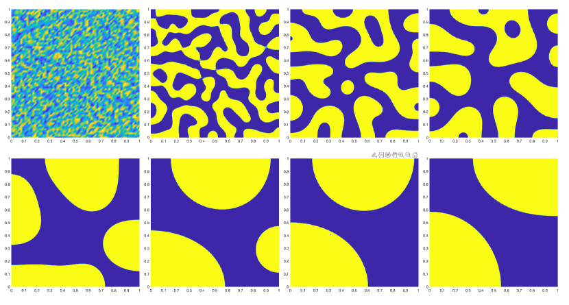
Figure 1: Snapshots of phase function at difference times from left to right row by row with $t=0,0.01,0.05,0.1,0.5,1,3,5,10s$, respectively.

5.3 Shape Relaxation with Rotational Boundary Condition

In this section, we present an example of shape relaxation within the domain $\Omega=(0,1)\times(0,1)$, where the boundary condition is set to $\mathbf{u}=(y-0.5,-x+0.5)$ on $\partial\Omega$. We evaluate the performance of the scheme described by (3.6)-(3.12) using critical phase field initial conditions. Specifically, we define $\phi^{0}=1$ within a polygonal subdomain featuring reentrant corners and $\phi^{0}=-1$ in the rest of $\Omega$. The initial velocity is given by $\mathbf{u}^{0}=(y-0.5,-x+0.5)$. This problem has been numerically studied in [4]. For our simulations, we adopt the following parameters: $M=0.001$, $\lambda=0.1$, $\epsilon=0.01$, $\nu=1$, and $T=0.5$. We solve the problem using scheme (3.6)-(3.12) with a $P_{2}$ element for $\phi_{h}^{n+1}$ and $\mu_{h}^{n+1}$, and a $P_{2}\times P_{1}$ element for $\mathbf{u}_{h}^{n+1}$ and $p_{h}^{n+1}$. We run the simulation up to $T=0.5$ and record the phase function snapshots at $t=0,0.01,0.05,0.08,0.1,0.2,0.3,0.5$, which are depicted in Figure 2. Our scheme is unconditionally energy stable in this example, as shown in Figure 3.

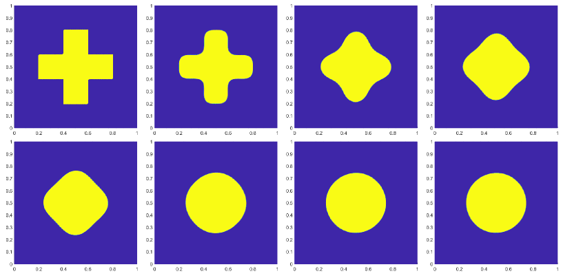
Figure 2: Snapshots of phase function at difference times from left to right row by row with $t=0,0.01,0.05,0.08,0.1,0.2,0.3,0.5$, respectively.

5.4 Comparison of time efficiency

In the subsection, we compare it with the following scheme [25] in the computation of the total time,

$$\left(\delta_{\tau}\phi_{h}^{n+1},w_{h}\right)+\left(\nabla\mu_{h}^{n+1},\nabla w_{h}\right)+b\left(\phi_{h}^{n},\mathbf{u}_{h}^{n+1},w_{h}\right)= 0,$$ (5.5)

$$\left(\nabla\phi_{h}^{n+1},\nabla\varphi_{h}\right)-\left(\mu_{h}^{n+1},\varphi_{h}\right)+\left((\phi_{h}^{n+1})^{3}-\phi_{h}^{n},\varphi_{h}\right)= 0,$$

$$\left(\delta_{\tau}\mathbf{u}_{h}^{n+1},\mathbf{v}_{h}\right)+\left(\nabla\mathbf{u}_{h}^{n+1},\nabla\mathbf{v}_{h}\right)+\bm{B}\left(\mathbf{u}_{h}^{n},\mathbf{u}_{h}^{n+1},\mathbf{v}_{h}\right)-\left(p_{h}^{n+1},\nabla\cdot\mathbf{v}_{h}\right)-b\left(\phi_{h}^{n},\mathbf{v}_{h},\mu_{h}^{n+1}\right)= 0,$$

$$\left(\nabla\cdot\mathbf{u}_{h}^{n+1},q_{h}\right)= 0.$$

By using the above scheme and our proposed scheme to the convergence tests of subsection 5.1, we obtain the time results in Table 3. The data in Table 3 shows that our algorithm takes 8.22 hour and the algorithm in [25] takes 23.18 hour, which is about 3 times faster in time than the scheme of [25]. Thus our scheme is more time efficient.

Table 3: Comparison of time consumed in different schemes.

Scheme	CPU Time (hour)
Cai et al. [25]	23.18
Our scheme	8.22

5.5 Lid driven cavity boundary condition

In the experiment, we take $\Omega=[0,1]^{2}$, $\epsilon=0.02$, $M=0.025$, $\nu=0.1$, $\lambda=0.001$, boundary condition on the top is $g=[1,0]$, initial condition for velocity is $\mathbf{u}_{0}=[1,0]$, $\tau=0.001,h=1/64$. We solve the problem using scheme (3.6)-(3.12) with the $P_{2}\times P_{2}\times P_{2}\times P_{1}$ for $\phi_{h}^{n+1}$, $\mu_{h}^{n+1}$, $\mathbf{u}_{h}^{n+1}$ and $p_{h}^{n+1}$, snapshots time $t=0,5,10,20,30,50$. The evolution of the concentration for this problem is shown through Figure 4 (see [41] for a similar problem).

Figure 3: Energy decay of our scheme in this example.

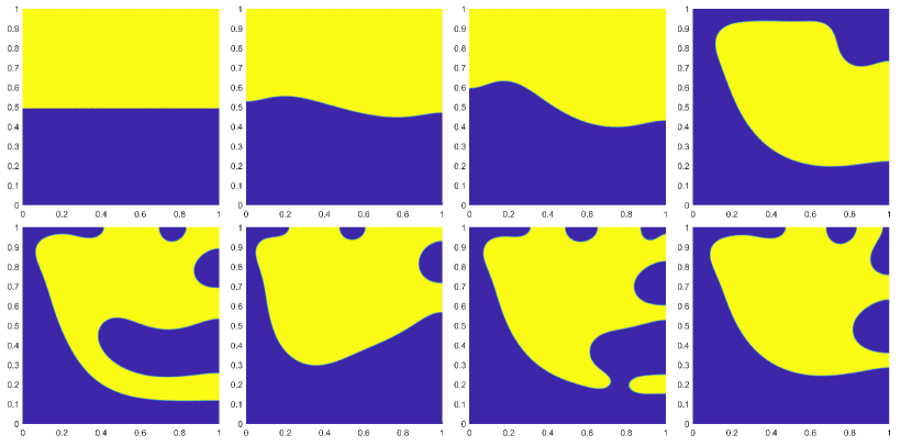
Figure 4: Evolution of the concentration with different time-step $\tau$.

5.6 Verification of energy stability

In this final test, we aim to verify the energy stability of the new scheme. We use the same settings as those in the coarsening dynamics test (see subsection 5.2), but with varying time steps $\tau$. As shown in Figure 5, our scheme demonstrates unconditional stability with respect to energy dissipation.

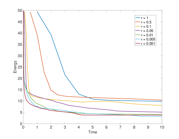
Figure 5: Evolution of the energy with different time-step $\tau$.

6 Conclusions

In this work, we propose a decoupling method for the Cahn–Hilliard–Navier–Stokes (CHNS) model, a highly coupled nonlinear system. The method, based on a convex-splitting approach, is first-order, fully discrete, and energy stable, making it efficient and easy to implement. Moreover, we have conducted a rigorous error analysis for the fully discrete scheme and derived optimal error estimates for all relevant functions in the $L^{2}$ norm. The presented numerical experiments are designed to verify the theoretical results of our method. It has been experimentally proven that our scheme is unconditionally stable, a property that has not been theoretically proven and requires further research.

References

• [1] Roger Temam. Navier-Stokes equations: Theory and numerical analysis, volume Vol. 2 of Studies in Mathematics and its Applications. North-Holland Publishing Co., Amsterdam-New York-Oxford, 1977.
• [2] John Cahn and John Hilliard. Free energy of a nonuniform system. I. Interfacial Free Energy. J. Chem. Phys., 28:258–267, 1958.
• [3] David Kay and Richard Welford. Efficient numerical solution of Cahn-Hilliard-Navier-Stokes fluids in 2D. SIAM J. Sci. Comput., 29(6):2241–2257, 2007.
• [4] David Kay, Vanessa Styles, and Richard Welford. Finite element approximation of a Cahn-Hilliard-Navier-Stokes system. Interfaces Free Bound., 10(1):15–43, 2008.
• [5] David Eyre. Unconditionally gradient stable time marching the Cahn-Hilliard equation. In Computational and mathematical models of microstructural evolution (San Francisco, CA, 1998), volume 529 of Mater. Res. Soc. Sympos. Proc., pages 39–46. MRS, Warrendale, PA, 1998.
• [6] Jie Shen and Xiaofeng Yang. Energy stable schemes for Cahn-Hilliard phase-field model of two-phase incompressible flows. Chinese Ann. Math. Ser. B, 31(5):743–758, 2010.
• [7] Xiaofeng Yang, Jia Zhao, and Qi Wang. Numerical approximations for the molecular beam epitaxial growth model based on the invariant energy quadratization method. J. Comput. Phys., 333:104–127, 2017.
• [8] Jie Shen, Jie Xu, and Jiang Yang. The scalar auxiliary variable (SAV) approach for gradient flows. J. Comput. Phys., 353:407–416, 2018.
• [9] Jie Shen and Jie Xu. Convergence and error analysis for the scalar auxiliary variable (SAV) schemes to gradient flows. SIAM J. Numer. Anal., 56(5):2895–2912, 2018.
• [10] Jean Luc Guermond, Peter Minev, and Jie Shen. An overview of projection methods for incompressible flows. Comput. Methods Appl. Mech. Engrg., 195(44-47):6011–6045, 2006.
• [11] Alexandre Joel Chorin. Numerical solution of the Navier-Stokes equations. Math. Comp., 22:745–762, 1968.
• [12] Amanda Diegel, Cheng Wang, Xiaoming Wang, and Steven Wise. Convergence analysis and error estimates for a second order accurate finite element method for the Cahn-Hilliard-Navier-Stokes system. Numer. Math., 137(3):495–534, 2017.
• [13] Cheng Wang, Jilu Wang, Steven M. Wise, Zeyu Xia, and Liwei Xu. Convergence analysis of a temporally second-order accurate finite element scheme for the Cahn-Hilliard-magnetohydrodynamics system of equations. J. Comput. Appl. Math., 436:Paper No. 115409, 17, 2024.
• [14] Daozhi Han and Xiaoming Wang. A second order in time, uniquely solvable, unconditionally stable numerical scheme for Cahn-Hilliard-Navier-Stokes equation. J. Comput. Phys., 290:139–156, 2015.
• [15] Jie Shen and Xiaofeng Yang. Decoupled, energy stable schemes for phase-field models of two-phase incompressible flows. SIAM J. Numer. Anal., 53(1):279–296, 2015.
• [16] Yongyong Cai and Jie Shen. Error estimates for a fully discretized scheme to a Cahn-Hilliard phase-field model for two-phase incompressible flows. Math. Comp., 87(313):2057–2090, 2018.
• [17] Yali Gao, Xiaoming He, Liquan Mei, and Xiaofeng Yang. Decoupled, linear, and energy stable finite element method for the Cahn-Hilliard-Navier-Stokes-Darcy phase field model. SIAM J. Sci. Comput., 40(1):B110–B137, 2018.
• [18] Lianlei Lin, Zhiguo Yang, and Suchuan Dong. Numerical approximation of incompressible Navier-Stokes equations based on an auxiliary energy variable. J. Comput. Phys., 388:1–22, 2019.
• [19] Hongen Jia, Xue Wang, and Kaitai Li. A novel linear, unconditional energy stable scheme for the incompressible Cahn-Hilliard-Navier-Stokes phase-field model. Comput. Math. Appl., 80(12):2948–2971, 2020.
• [20] Zhen Xu, Xiaofeng Yang, and Hui Zhang. Error analysis of a decoupled, linear stabilization scheme for the Cahn-Hilliard model of two-phase incompressible flows. J. Sci. Comput., 83(3):Paper No. 57, 27, 2020.
• [21] Guodong Zhang, Xiaoming He, and Xiaofeng Yang. Decoupled, linear, and unconditionally energy stable fully discrete finite element numerical scheme for a two-phase ferrohydrodynamics model. SIAM J. Sci. Comput., 43(1):B167–B193, 2021.
• [22] Xiaoli Li and Jie Shen. On fully decoupled MSAV schemes for the Cahn-Hilliard-Navier-Stokes model of two-phase incompressible flows. Math. Models Methods Appl. Sci., 32(3):457–495, 2022.
• [23] Wenbin Chen, Jianyu Jing, Qianqian Liu, Cheng Wang, and Xiaoming Wang. Convergence analysis of a second order numerical scheme for the Flory-Huggins-Cahn-Hilliard-Navier-Stokes system. J. Comput. Appl. Math., 450:Paper No. 115981, 22, 2024.
• [24] Juan Wen, Yinnian He, and Yaling He. Semi-implicit, unconditionally energy stable, stabilized finite element method based on multiscale enrichment for the cahn-hilliard-navier-stokes phase-field model. Computers and Mathematics with Applications, 126:172–181, 2022.
• [25] Wentao Cai, Weiwei Sun, Jilu Wang, and Zongze Yang. Optimal $L^{2}$ error estimates of unconditionally stable finite element schemes for the Cahn-Hilliard-Navier-Stokes system. SIAM J. Numer. Anal., 61(3):1218–1245, 2023.
• [26] Jinting Yang and Nianyu Yi. Convergence analysis of a decoupled pressure-correction SAV-FEM for the Cahn–Hilliard–Navier–Stokes model. J. Comput. Appl. Math., 449:Paper No. 115985, 2024.
• [27] Douglas Arnold, Franco Brezzi, and Michel Fortin. A stable finite element for the Stokes equations. Calcolo, 21(4):337–344, 1984.
• [28] John G Heywood and Rolf Rannacher. Finite-element approximation of the nonstationary Navier-Stokes problem. IV. Error analysis for second-order time discretization. SIAM J. Numer. Anal., 27(2):353–384, 1990.
• [29] Amanda Diegel, Xiaobing Feng, and Steven Wise. Analysis of a mixed finite element method for a Cahn-Hilliard-Darcy-Stokes system. SIAM J. Numer. Anal., 53(1):127–152, 2015.
• [30] Mary Fanett Wheeler. A priori $L_{2}$ error estimates for Galerkin approximations to parabolic partial differential equations. SIAM J. Numer. Anal., 10:723–759, 1973.
• [31] Susanne Brenner and Ridgway Scott. The mathematical theory of finite element methods, volume 15 of Texts in Applied Mathematics. Springer, New York, third edition, 2008.
• [32] Thomas Yizhao Hou and Zuoqiang Shi. An efficient semi-implicit immersed boundary method for the Navier-Stokes equations. J. Comput. Phys., 227(20):8968–8991, 2008.
• [33] Yinnian He. Unconditional convergence of the Euler semi-implicit scheme for the three-dimensional incompressible MHD equations. IMA J. Numer. Anal., 35(2):767–801, 2015.
• [34] Vivette Girault and Pierre Arnaud Raviart. Finite element methods for Navier-Stokes equations, volume 5 of Springer Series in Computational Mathematics. Springer-Verlag, Berlin, 1986. Theory and algorithms.
• [35] Vidar Thomée. Galerkin finite element methods for parabolic problems, volume 25 of Springer Series in Computational Mathematics. Springer-Verlag, Berlin, second edition, 2006.
• [36] Xiaofeng Yang, Guodong Zhang, and Xiaoming He. Convergence analysis of an unconditionally energy stable projection scheme for magneto-hydrodynamic equations. Appl. Numer. Math., 136:235–256, 2019.
• [37] Hongtao Chen, Jingjing Mao, and Jie Shen. Optimal error estimates for the scalar auxiliary variable finite-element schemes for gradient flows. Numer. Math., 145(1):167–196, 2020.
• [38] Xiaobing Feng. Fully discrete finite element approximations of the Navier-Stokes-Cahn-Hilliard diffuse interface model for two-phase fluid flows. SIAM J. Numer. Anal., 44(3):1049–1072, 2006.
• [39] Yinnian He and Weiwei Sun. Stability and convergence of the Crank-Nicolson/Adams-Bashforth scheme for the time-dependent Navier-Stokes equations. SIAM J. Numer. Anal., 45(2):837–869, 2007.
• [40] Yaoyao Chen, Yunqing Huang, and Nianyu Yi. Error analysis of a decoupled, linear and stable finite element method for Cahn-Hilliard-Navier-Stokes equations. Appl. Math. Comput., 421:Paper No. 126928, 17, 2022.
• [41] Franck Boyer. A theoretical and numerical model for the study of incompressible mixture flows. Computers & Fluids, 31(1):41–68, 2002.