Nontrivial damping of magnetization currents in perturbed spin chains

Abstract

Since perturbations are omnipresent in physics, understanding their impact on the dynamics of quantum many-body systems is a vitally important but notoriously difficult question. On the one hand, random-matrix and typicality arguments suggest a rather simple damping in the overwhelming majority of cases, e.g., exponential damping according to Fermi’s Golden Rule. On the other hand, counterexamples are known to exist, and it remains unclear how frequent and under which conditions such counterexamples appear. In our work, we consider the spin-1/2 XXZ chain as a paradigmatic example of a quantum many-body system and study the dynamics of the magnetization current in the easy-axis regime. Using numerical simulations based on dynamical quantum typicality, we show that the standard autocorrelation function is damped in a nontrivial way and that only a modified version of this function is damped in a simple manner. Employing projection-operator techniques in addition, we demonstrate that both, the nontrivial and simple damping relation can be understood on perturbative grounds. Our results are in agreement with earlier findings for the particle current in the Hubbard chain.

I Introduction

Quantum many-body systems out of equilibrium continue to be a central topic of modern research and are relevant to a broad class of physical situations. These situations range from strictly isolated quantum systems to open or driven quantum systems explicitly coupled to external baths or forces. In particular, substantial progress has been made in recent years [1, 2, 3, 4, 5, 6, 7, 8, 9, 10, 11], not least due to the advance of controlled experimental platforms, the development of powerful numerical techniques, and the invention of fresh theoretical concepts.

Within the diverse questions, a key issue is the equilibration and thermalization of closed quantum systems. Here, the fundamental question arises whether a system will eventually reach thermal equilibrium. A main ansatz is the eigenstate thermalization hypothesis (ETH) [12, 13, 14], which provides a microscopic explanation for the emergence of thermalization and is closely related to random-matrix theory. Moreover, equally important questions are the actual time scales of equilibration and the specific form of the relaxation process [15, 16, 17, 18, 19, 20, 21, 22, 23].

In this context, an intriguing question is how the relaxation process is altered if the system’s Hamiltonian $H$ is affected by the presence of a perturbation $V$ of some strength $\epsilon$ [24, 25, 26, 27, 28, 29, 30, 31, 32],

$$H=H_{0}+\epsilon V\,.$$ (1)

In general, this question is notoriously difficult to answer and the effect of such a perturbation can be manifold. However, random-matrix and typicality arguments suggest a rather simple damping in the vast majority of cases [33, 34, 35], e.g., exponential according to Fermi’s Golden Rule,

$$f_{\varepsilon}(t)=f_{\varepsilon=0}(t)\,e^{-\varepsilon^{2}\gamma t}\,.$$ (2)

Still, counterexamples are known to exist [36], and it remains unclear how frequent and under which conditions such counterexamples appear [37].

In our work, we discuss this impact of perturbations on the dynamics of quantum many-body systems, with the focus on the magnetization current in the spin-$1/2$ XXZ chain, serving as a paradigmatic example for observable and model [7]. In particular, we study the damping of the current autocorrelation function for two distinct choices of reference systems, where the first one is noninteracting [38, 39] and second one is interacting [40, 41, 42, 43]. To this end, we use numerical simulations based on the concept of dynamical quantum typicality [44, 45, 46, 47, 48, 49, 50, 51, 52, 53, 54, 55, 56, 57, 58], in order to obtain exact results for systems of comparatively large but still finite size. We complement these results by further results from a lowest-order perturbation theory on the basis of the time-convolutionless (TCL) projection-operator technique [59, 60].

For the noninteracting reference system, we find an exponential damping, which is consistent with other works. For the interacting reference system, however, we show that the standard autocorrelation function is damped in a nontrivial way and only a modified version of it is damped in a simple manner. We demonstrate that both, the nontrivial and simple damping can be also understood on perturbative grounds. Our results are in agreement with earlier findings for the particle current in the Hubbard chain [36], and they suggest that nontrivial damping occurs if the unperturbed system already has a rich dynamical behavior.

This paper is structured as follows. In Sec. II, we first introduce the models studied, i.e., the integrable spin-$1/2$ XXZ chain and its nonintegrable version with next-nearest-neighbor interactions. Additionally, we define the perturbation scenarios considered as well as the magnetization current as the observable of interest. In this context, we also introduce the standard autocorrelation function in the limit of high temperatures. In Sec. III, we turn to the TCL projection-operator technique as our perturbative approach to the relaxation process, focusing on the general framework in Sec. III.1. In Sec. III.2, a specific choice of a projection is discussed, which has been used in previous works to access a modified version of the standard current autocorrelation function. A main extension of our work is presented in Sec. III.3, where we introduce another projection to connect to the desired standard current autocorrelation function. Then, we turn to our results in Sec. IV and provide a comparison between exact data and our TCL results. We present our results for the noninteracting reference system in Sec. IV.1 and for the interacting reference system in Sec. IV.2. In Sec. V, we summarize our work and draw conclusions.

II Model and observable

Although our main question is of relevance to a broad class of quantum many-body systems, we focus here on the spin-$1/2$ XXZ chain, which is a paradigmatic example and has attracted significant attention in the literature before [7]. This model is given by the Hamiltonian

$$H_{\text{XXZ}}=J\sum_{r=1}^{L}(S_{r}^{x}S_{r+1}^{x}+S_{r}^{y}S_{r+1}^{y}+\Delta S_{r}^{z}S_{r+1}^{z})\,,$$ (3)

where $S_{r}^{i}$ ($i=x$, $y$, $z$) are the components of a spin-$1/2$ operator at lattice site $r$, $L$ is the total number of lattice sites, $J$ is the exchange coupling constant, and $\Delta$ is the anisotropy in $z$ direction. Throughout our work, we use periodic boundary conditions, i.e., $S_{L+1}^{i}=S_{1}^{i}$. Since the spin-$1/2$ XXZ chain is Bethe-Ansatz integrable for any value of the anisotropy $\Delta$, we break this integrability by an additional interaction between next-nearest sites,

$$H=H_{\text{XXZ}}+J\Delta^{\prime}\sum_{r=1}^{L}S_{r}^{z}S_{r+2}^{z}\,,$$ (4)

where $\Delta^{\prime}$ is the interaction strength. As will be discussed later, this interaction will play the role of a perturbation. The model is sketched in Fig. 1.

For all choices of $\Delta$ and $\Delta^{\prime}$, the total magnetization $S^{z}=\sum_{r}S^{z}_{r}$ is conserved, $[S^{z},H]=0$. As a consequence, the temporal change of a local magnetization is related to a flow of local currents,

$$\frac{\text{d}}{\text{d}t}S_{r}^{z}=i[H,S_{r}^{z}]=j_{r-1}-j_{r}\,,$$ (5)

which then leads to the well-known definition of the total current [7]

$$j=J\sum_{r=1}^{L}j_{r}\,,\quad j_{r}=J(S_{r}^{x}S_{r+1}^{y}-S_{r}^{y}S_{r+1}^{x})\,.$$ (6)

While the total current $j$ itself does not depend on $\Delta$ or $\Delta^{\prime}$, its dynamics does. In particular, only in the case $\Delta=\Delta^{\prime}=0$, $j$ is conserved, $[j,H]=0$. In general, one has $\text{tr}[j]=0$ and $\text{tr}[j^{2}]=LdJ^{2}/8$, where $d=2^{L}$ is the dimension of the Hilbert space.

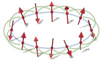
Figure 1: Sketch of the spin chain, as defined in Eq. (4), with periodic boundary conditions and interactions between both, nearest (blue) and next-nearest (green) neighbors.

Within the framework of linear response theory [61], transport properties are related to the autocorrelation function of $j$ at equilibrium,

$$\langle j(t)j(0)\rangle_{\text{eq}}=\frac{\text{tr}[\mathrm{e}^{-\beta H}\mathrm{e}^{iHt}j\mathrm{e}^{-iHt}j]}{Z}\,,$$ (7)

with the partition function $Z=\text{tr}[\mathrm{e}^{-\beta H}]$ at the inverse temperature $\beta=1/T$. For the remainder of our work, we focus on the limit of high temperatures,

$$C_{S}(t)=\lim_{\beta\to 0}\langle j(t)j(0)\rangle_{\text{eq}}=\frac{\text{tr}[\mathrm{e}^{iHt}j\mathrm{e}^{-iHt}j]}{d}\,,$$ (8)

where $d$ denotes again the Hilbert-space dimension. Even in this limit, the time evolution of the autocorrelation function $C_{S}(t)$ is nontrivial. Note that an index $S$ is used to indicate a standard correlation function and another index $M$ is used later to indicate a modified correlation function.

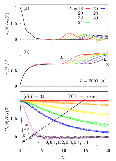
Figure 2: Noninteracting reference system $H_{0}$ with $\Delta=0$ and $\Delta^{\prime}=0$. (a) Second-order kernel $k_{2}(t)$ and (b) corresponding rate $\gamma_{2}(t)$, both for various system sizes $L\leq 30$. (c) Resulting prediction for the current autocorrelation function $C_{S}(t)$ and exact numerical results for various perturbation strengths $\varepsilon$, both for a fixed system size $L=30$. In (b), we also depict a $L=2000$ data point from Ref. [39].

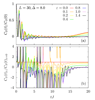
Figure 3: Interacting reference system $H_{0}$ with $\Delta=8.0$ and $\Delta^{\prime}=0$. (a) Exact dynamics of the autocorrelation function $C_{S}(t)$ for various perturbation strengths $\varepsilon$ and fixed system size $L=30$. (b) Ratio between perturbed and unperturbed autocorrelation functions.

Since we are interested in the impact of a perturbation on the dynamics of the autocorrelation function $C_{S}(t)$, we express the full Hamiltonian as

$$H=H_{0}+\varepsilon V\,,$$ (9)

where $H_{0}$ is the unperturbed Hamiltonian and $\varepsilon V$ is a perturbation of strength $\varepsilon$, which can be weak but also strong. Specifically, we consider two different scenarios in our work. (i) The reference Hamiltonian

$$H_{0}=H(\Delta=\Delta^{\prime}=0)$$ (10)

is noninteracting and the perturbation

$$V=J\sum_{r=1}^{L}(S_{r}^{z}S_{r+1}^{z}+S_{r}^{z}S_{r+2}^{z})\,,\quad\varepsilon=\Delta=\Delta^{\prime}$$ (11)

contains all interactions. (ii) The reference Hamiltonian is changed into

$$H_{0}=H(\Delta\neq 0,\Delta^{\prime}=0)$$ (12)

and also includes interactions between nearest sites, while the perturbation

$$V=J\sum_{r=1}^{L}S_{r}^{z}S_{r+2}^{z}\,,\quad\varepsilon=\Delta^{\prime}$$ (13)

consists of the other interactions between next-nearest sites. In the scenario (i), the total current $j$ is conserved in the unperturbed system $H_{0}$, $[j,H_{0}]=0$. Hence, the autocorrelation function becomes

$$C_{S}(t)=\text{const.}$$ (14)

for $\varepsilon=0$ and has no dynamics at all. In contrast, in the scenario (ii), $[j,H_{0}]\neq 0$. Therefore, the autocorrelation function becomes

$$C_{S}(t)\neq\text{const.}$$ (15)

for $\varepsilon=0$ and has a dynamics, which can be also rich for large anisotropies $\Delta\gg 1$ [62].

For both scenarios, we study the change of $C_{S}(t)$ with $\varepsilon$, using numerical simulations based on the concept of dynamical quantum typicality [56, 57]. This concept allows us to treat finite systems of sizes up to $L=30$, where the Hilbert-space dimension is $D={\cal O}(10^{9})$. These exact numerical simulations are complemented by perturbative approaches, which will be introduced below.

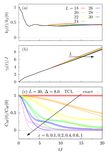
Figure 4: Interacting reference system $H_{0}$ with $\Delta=8.0$ and $\Delta^{\prime}=0$. (a) Second-order kernel $k_{2}(t)$ and (b) corresponding rate $\gamma_{2}(t)$, both for various system sizes $L\leq 30$. (c) Resulting prediction for the modified current autocorrelation function $C_{M}(t)$ and exact numerical results for various perturbation strengths $\varepsilon$, both for a fixed system size $L=30$.

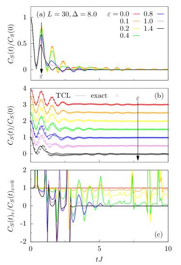
Figure 5: Interacting reference system $H_{0}$ with $\Delta=8.0$ and $\Delta^{\prime}=0$. (a) Second-order prediction for the dynamics of the standard current autocorrelation function $C_{S}(t)$ for various perturbation strengths $\varepsilon$ and a fixed system size $L=30$. (b) Comparison of (a) with the exact dynamics, where data is shifted for better visibility. (c) Ratio between perturbed and unperturbed time evolution in (a).

III Projection-operator techniques

III.1 Framework

Next, we turn to our perturbative approaches, which rely on projection-operator techniques. These techniques can be applied to the scenario in Eq. (9), where the full Hamiltonian $H$ is decomposed into a reference system $H_{0}$ and a perturbation $V$.

The cental idea of projection-operator techniques is to reduce the complete microscopic dynamics to equations of motion for a set of relevant variables, which should at least include the observable of interest. To this end, one formally defines a projection (super)operator

$$\mathcal{P}\rho(t)=\sum_{i=1}^{N}\frac{\text{tr}[P_{i}\,\rho(t)]}{\text{tr}[(P_{i})^{2}]}\,,$$ (16)

where $\rho(t)$ is the time-dependent density matrix and the operators $P_{i}$ are orthogonal to each other,

$$\text{tr}[P_{i}P_{j}]=\text{tr}[(P_{i})^{2}]\,\delta_{i,j}\,.$$ (17)

Therefore, ${\cal P}^{2}={\cal P}$. Throughout our work, we consider initial states

$$\rho(0)=\text{span}[P_{1},P_{2},\ldots,P_{N}]$$ (18)

such that $(1-{\cal P})\rho(0)=0$.

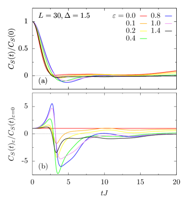
Figure 6: Interacting reference system $H_{0}$ with $\Delta=1.5$ and $\Delta^{\prime}=0$. (a) Exact dynamics of the autocorrelation function $C_{S}(t)$ for various perturbation strengths $\varepsilon$ and fixed system size $L=30$. (b) Ratio between perturbed and unperturbed autocorrelation functions.

Once the decomposition in Eq. (9) and the projection operator in Eq. (16) are chosen, the time-convolutionless (TCL) projection-operator technique [59, 60] then leads to a time-local differential equation of the form

$$\frac{\text{d}}{\text{d}t}\mathcal{P}\rho_{\text{I}}(t)=\mathcal{G}(t)\mathcal{P}\rho_{\text{I}}(t)+\mathcal{I}(t)(1-\mathcal{P})\rho(0)$$ (19)

and avoids the often troublesome time convolution in the context of the Nakajima-Zwanzig formalism. Here, $\rho_{\text{I}}(t)$ is the time-dependent density matrix in the interaction picture,

$$\rho_{\text{I}}(t)=e^{iH_{0}t}e^{-iHt}\rho(0)e^{iHt}e^{-iH_{0}t}\,,$$ (20)

and the inhomogeneity ${\cal I}(t)$ can be neglected, due to our choice of initial conditions. The generator $\mathcal{G}(t)$ is given as a systematic perturbation expansion in powers of the perturbation strength $\varepsilon$,

$${\cal G}(t)=\sum_{i=1}^{\infty}\varepsilon^{i}\,{\cal G}_{i}(t)\,,\quad{\cal G}_{2i-1}(t)=0\,,$$ (21)

where odd contributions of the expansion vanish in many cases, as for our choice below. Hence, the lowest order is the second order and reads

$$\mathcal{G}_{2}(t)=\varepsilon^{2}\int_{0}^{t}\mathrm{d}t^{\prime}\,\mathcal{P}\mathcal{L}(t)\mathcal{L}(t^{\prime})\mathcal{P}\,,$$ (22)

where the Liouvillian is given by

$$\mathcal{L}(t)\bullet=-i[V_{\text{I}}(t),\bullet]\,,\quad V_{\text{I}}(t)=e^{iH_{0}t}V(0)e^{-iH_{0}t}\,.$$ (23)

Our central assumption is a corresponding truncation to this second order. Thus, we rely on

$$\frac{\text{d}}{\text{d}t}\mathcal{P}\rho_{\text{I}}(t)=\mathcal{G}_{2}(t)\mathcal{P}\rho_{\text{I}}(t)\,.$$ (24)

In general, the quality of such a truncation depends on the strength of $\varepsilon$, the structure of $V$, and the choice of ${\cal P}$. Naturally, the quality can be also improved by taking into account higher-order corrections. For the purposes of our work, however, the second-order truncation will be sufficient.

In the following, we elaborate on the lowest-order TCL description in Eq. (24). We do so for two different choices of the projection operator. The first projection is based on a previous work [36] and yields to a prediction for a modified autocorrelation function $C_{M}(t)$, which differs from the standard autocorrelation function $C_{S}(t)$. The second projection aims at a perturbative description of the actual $C_{S}(t)$.

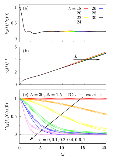
Figure 7: Interacting reference system $H_{0}$ with $\Delta=1.5$ and $\Delta^{\prime}=0$. (a) Second-order kernel $k_{2}(t)$ and (b) corresponding rate $\gamma_{2}(t)$, both for various system sizes $L\leq 30$. (c) Resulting prediction for the modified current autocorrelation function $C_{M}(t)$ and exact numerical results for various perturbation strengths $\varepsilon$, both for a fixed system size $L=30$.

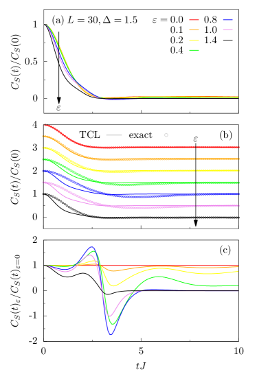
Figure 8: Interacting reference system $H_{0}$ with $\Delta=1.5$ and $\Delta^{\prime}=0$. (a) Second-order prediction for the dynamics of the standard current autocorrelation function $C_{S}(t)$ for various perturbation strengths $\varepsilon$ and a fixed system size $L=30$. (b) Comparison of (a) with the exact dynamics, where data is shifted for better visibility. (c) Ratio between perturbed and unperturbed time evolution in (a).

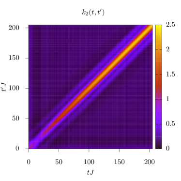
Figure 9: Density plot of the second-order TCL kernel $k_{2}(t,t^{\prime})$ in Eq. (30) for an interacting reference $H_{0}$ with $\Delta=1.5$ and $\Delta^{\prime}=0$ and system size of $L=30$. A clear diagonal structure is visible.

III.2 Simple projection and modified correlation function

As done in a previous work [36], we first choose for the projection only two operators, i.e., the identity $1$ and the total current $j$. Thus, the projection reads

$$\mathcal{P}\rho_{\text{I}}(t)=\frac{1}{d}+\frac{C_{M}(t)}{\text{tr}[j^{2}]}\,j\,,\quad C_{M}(t)=\text{tr}[j\rho_{\text{I}}(t)]\,,$$ (25)

where $C_{M}(t)$ is the time-dependent part of the projected density matrix. For initial states

$$\rho(0)=\frac{1+\alpha j}{d}\,,$$ (26)

this time-dependent part becomes

$$C_{M}(t)=\alpha\,\frac{\text{tr}[\mathrm{e}^{iHt}j\mathrm{e}^{-iHt}\mathrm{e}^{iH_{0}t}j\mathrm{e}^{-iH_{0}t}]}{d}$$ (27)

and then takes on the form of a current autocorrelation function. Yet, compared to the standard one in Eq. (8), it is modified: While one $j$ evolves w.r.t. $H$, the other $j$ evolves w.r.t. $H_{0}$. To indicate this difference, we use the index $M$.

For the projection in Eq. (25), the second-order TCL description in Eq. (24) leads to the rate equation

$$\frac{\text{d}}{\text{d}t}\,C_{M}(t)=-\varepsilon^{2}\,\gamma_{2}(t)\,C_{M}(t)\,,$$ (28)

where the time-dependent rate

$$\gamma_{2}(t)=\int_{0}^{t}\text{d}t^{\prime}\,k_{2}(t,t^{\prime})$$ (29)

is given as an time integral over the kernel

$$k_{2}(t,t^{\prime})=\frac{\text{tr}(i[j,V_{I}(t)]\,i[j,V_{I}(t^{\prime})])}{\text{tr}(j^{2})}\,.$$ (30)

It is convenient to assume that $k_{2}(t,t^{\prime})=k_{2}(t-t^{\prime})$, which is only exact for $[j,H_{0}]=0$. This assumption is discussed in Appendix B.

Obviously, Eq. (28) is solved via an exponential decay of the form

$$\frac{C_{M}(t)}{C_{M}(0)}=\exp\Big{[}-\varepsilon^{2}\!\int_{0}^{t}\text{d}t^{\prime}\,\gamma_{2}(t^{\prime})\Big{]}\,,$$ (31)

with a generally time-dependent rate $\gamma_{2}(t)$. However, if the underlying kernel $k_{2}(t-t^{\prime})$ decays to zero on a certain time scale, $\gamma_{2}(t)$ becomes constant after this time scale. Then, the earlier time dependence of $\gamma_{2}(t)$ can be neglected in the case of a small perturbation strength $\varepsilon$ and a slow relaxation process.

Overall, as a consequence of the solution in Eq. (31), one obtains a simple damping relation for the modified current autocorrelation function,

$$\frac{C_{M}(t)_{\varepsilon}}{C_{M}(t)_{\varepsilon=0}}=\exp\Big{[}-\varepsilon^{2}\!\int_{0}^{t}\text{d}t^{\prime}\,\gamma_{2}(t^{\prime})\Big{]}\,.$$ (32)

Importantly, this relation does not necessarily carry over to the standard current autocorrelation function,

$$\frac{C_{S}(t)_{\varepsilon}}{C_{S}(t)_{\varepsilon=0}}\neq\frac{C_{M}(t)_{\varepsilon}}{C_{M}(t)_{\varepsilon=0}}\,,$$ (33)

since both functions are only identical for $[j,H_{0}]=0$. This fact has been demonstrated by numerical simulations of the onedimensional Hubbard model [36], where $C_{S}(t)$ has a nontrivial damping relation for an interacting reference system, in contrast to $C_{M}(t)$. Later, we will demonstrate a similar behavior for the spin-$1/2$ XXZ chain.

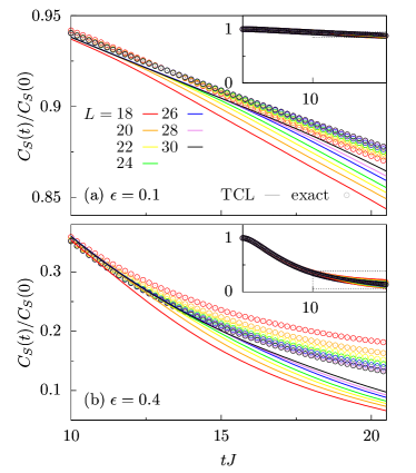
Figure 10: Noninteracting reference system $H_{0}$ with $\Delta=0$ and $\Delta^{\prime}=0$. Finite-size scaling of the current autocorrelation function $C_{S}(t)$ for perturbation strengths (a) $\varepsilon=0.1$ and (b) $\varepsilon=0.4$. Second-order TCL is compared to exact numerical simulations. Insets: Different plot range. Here, also the plot region of the main panels is indicated.

III.3 Extended projection and standard correlation function

So far, our choice of the projection $\mathcal{P}$ in Eq. (25) allows us to obtain a perturbative description for the modified current autocorrelation function $C_{M}(t)$, but not for the standard current autocorrelation function $C_{S}(t)$. Hence, we go beyond previous works and change the projection in a suitable way. The basic idea is an extension of the projection by a third operator $P_{3}$, while the already used operators $P_{1}=1$ and $P_{2}=j$ are kept. Specifically, we choose

$$P_{3}=j_{\tau}=e^{iH_{0}\tau}je^{-iH_{0}\tau}\,,$$ (34)

which is the time evolution of $j$ w.r.t. $H_{0}$. Here, $\tau$ is an arbitrary but fixed parameter. While $j_{\tau}$ is orthogonal to $P_{1}=1$, it is not orthogonal to $P_{2}=j$. Therefore, we change the second operator into

$$P_{2}=j^{\prime}=j-\frac{\text{tr}[j_{\tau}j]}{\text{tr}[(j_{\tau})^{2}]}\,j_{\tau}\,.$$ (35)

Thus, the extended projection reads

$$\mathcal{P}\rho_{\text{I}}(t)=\frac{1}{d}+\frac{a(t)}{\text{tr}[(j_{\tau})^{2})]}\,j_{\tau}+\frac{b(t)}{\text{tr}[(j^{\prime})^{2}]}\,j^{\prime}$$ (36)

with the time-dependent parts

$$a(t)=\text{tr}[j_{\tau}\rho_{\text{I}}(t)]\,,\quad b(t)=\text{tr}[j^{\prime}\rho_{\text{I}}(t)]\,.$$ (37)

Using the initial condition $\rho(0)$ in Eq. (26), one finds

$$a(t)=\alpha\,\frac{\text{tr}[e^{-iH_{0}t}j_{\tau}e^{iH_{0}t}e^{-iHt}je^{iHt}]}{d}$$ (38)

and, evaluated at $t=\tau$,

$$a(\tau)=\alpha\,C_{S}(\tau)\,.$$ (39)

Similarly, one finds

$$b(\tau)=\alpha\left[C_{M}(\tau)-\frac{C_{S}(\tau)_{\varepsilon=0}}{C_{S}(0)_{\varepsilon=0}}\,C_{S}(\tau)\right]\,.$$ (40)

Hence, $a(\tau)$ is directly connected to the desired standard current autocorrelation function $C_{S}(t)$, while $b(\tau$) is also related to the modified current autocorrelation function $C_{M}(t)$.

For the projection in Eq. (36), the second-order TCL description in Eq. (24) leads to the rate equation

$$\frac{\text{d}}{\text{d}t}\begin{pmatrix}a(t)\\ b(t)\end{pmatrix}=-\varepsilon^{2}\,\Gamma_{2}(t)\begin{pmatrix}a(t)\\ b(t)\end{pmatrix}\,,$$ (41)

which now becomes twodimensional. In particular, $a(t)$ and $b(t)$ are coupled via a time-dependent rate matrix $\Gamma_{2}(t)$. Similarly as before, this rate matrix is given as a time integral over an kernel,

$$\Gamma_{2}(t)=\int_{0}^{t}\text{d}t^{\prime}\,K_{2}(t,t^{\prime})\,,$$ (42)

where the matrix elements of the kernel are given by

$$K_{2,(1,1)}(t,t^{\prime})=\frac{\text{tr}(j_{\tau}[V_{I}(t),[V_{I}(t^{\prime}),j_{\tau}]])}{\text{tr}([j_{\tau}]^{2})}\,,$$ (43)

$$K_{2,(1,2)}(t,t^{\prime})=\frac{\text{tr}(j_{\tau}[V_{I}(t),[V_{I}(t^{\prime}),j^{\prime}]])}{\text{tr}([j^{\prime}]^{2})}\,,$$ (44)

$$K_{2,(2,1)}(t,t^{\prime})=\frac{\text{tr}(j^{\prime}[V_{I}(t),[V_{I}(t^{\prime}),j_{\tau}]])}{\text{tr}([j_{\tau}]^{2})}\,,$$ (45)

$$K_{2,(2,2)}(t,t^{\prime})=\frac{\text{tr}(j^{\prime}[V_{I}(t),[V_{I}(t^{\prime}),j^{\prime}]])}{\text{tr}([j^{\prime}]^{2})}\,.$$ (46)

and we assume that $K_{2}(t,t^{\prime})=K_{2}(t-t^{\prime})$.

Because the time dependence of the kernel $K_{2}(t,t^{\prime})$ is generated by the unperturbed system $H_{0}$ only, it is in principle possible to carry out the perturbation theory analytically. However, $H_{0}$ must be solved exactly, which can be challenging despite the Bethe-Ansatz integrability of the spin-$1/2$ XXZ chain. Therefore, we carry out the perturbation theory numerically, using again the concept of dynamical quantum typicality [56, 57]. In comparison to standard applications, the present implementation turns out to be more complex. Details on this implementation can be found in Appendix D.

IV Results

In the following, we turn to our numerical simulations for the current autocorrelation function in the perturbed spin-$1/2$ XXZ chain, where we cover two different choices of the reference system. In Sec. IV.1, we start with the noninteracting reference system and particularly connect to existing results in the literature. In Sec. IV.2, we move forward to the interacting reference system, which is the central case in our work.

IV.1 Noninteracting reference system

Let us start with the noninteracting reference system $H_{0}=H(\Delta=\Delta^{\prime}=0)$, where the perturbation $V$ consists of interactions between both, nearest and next-nearest sites. The strength of these two interactions is chosen to be the same, $\varepsilon=\Delta=\Delta^{\prime}$. Since in the non-interacting reference system the current is conserved, $[j,H_{0}]=0$, the dynamics of the current autocorrelation function is induced solely by the perturbation. The conservation of the current in the noninteracting reference system also implies that the standard and modified current-current correlation functions are identical,

$$C_{S}(t)=C_{M}(t)\,.$$ (47)

Thus, we do not distinguish between them here.

In Fig. 2 (c), we summarize the temporal decay of the current autocorrelation function $C_{S}(t)$ for a fixed system size $L=30$ and various perturbation strengths $\varepsilon$. Here, we particularly compare data from exact simulations on the basis of dynamical quantum typicality to data from second-order TCL. The overall agreement between the data is convincing for all values of $\varepsilon$ depicted. Although deviations become visible for strong perturbations, the rough shape of the two decay curves is still similar, which is remarkable in view of the second-order truncation of TCL. A comparison for other system sizes can be found in Appendix C.

It is also instructive to show data for the second-order kernel $k_{2}(t)$ and rate $\gamma_{2}(t)$. The kernel $k_{2}(t)$ in Fig. 2 (a) decays quickly and remains close to zero, until finite-size effects become relevant. Consequently, the rate $\gamma_{2}(t)$ in Fig. 2 (b) quickly saturates at a constant plateau value, until the same finite-size effects set in. While the plateau value does not change significantly with system size, the plateau length increases gradually. Therefore, already on the basis of data for system sizes $L\leq 30$, one can conclude on the thermodynamic limit. And indeed, the plateau value for $L\leq 30$ is consistent with the one for $L=2000$ in Ref. [39], where an analytical expression has been derived. Such a derivation is feasible, because of the noninteracting reference system.

Let us briefly comment on the functional form of the decay curve of the current autocorrelation function. Due to the saturation of the rate $\gamma_{2}(t)$ at a constant plateau value, this decay curve is exponential for small $\varepsilon$, where the relevant time scale is long and the initial increase of $\gamma_{2}(t)$ can be neglected. For large $\varepsilon$, however, the relevant time scale becomes short and the initial increase of $\gamma_{2}(t)$ is relevant. Since $\gamma_{2}(t)$ increases linearly, the decay curve then turns into a Gaussian, which is consistent with the numerical simulations in Fig. 2 (c).

IV.2 Interacting reference system

Now, we are ready to come to the central part of our work, where we consider an interacting reference system $H_{0}=H(\Delta\neq 0,\Delta^{\prime}=0)$. Because the reference system now includes also interactions between nearest sites, the role of the perturbation $V$ is only played by interactions between next-nearest sites. In the interacting reference system, the current is no longer conserved, $[j,H_{0}]\neq 0$, and the standard and modified current autocorrelation functions differ,

$$C_{S}(t)\neq C_{M}(t)\,.$$ (48)

Here, we focus on a large anisotropy $\Delta=8.0$, where this difference is pronounced. Other values of the anisotropy are discussed in Appendix A.

In Fig. 3 (a), we first summarize the temporal decay of the standard current autocorrelation function $C_{S}(t)$, as obtained from exact numerical simulations. We do so for a fixed system size $L=30$ and various perturbation strengths $\varepsilon$. While $C_{S}(t)$ is damped, it additionally has oscillations, where frequencies and zero crossings depend on $\varepsilon$. In particular, there is no obvious damping relation between the perturbed and unperturbed dynamics. This observation becomes evident from the ratio

$$C_{S}(t)_{\varepsilon}/C_{S}(t)_{\varepsilon=0}\,,$$ (49)

as shown in Fig. 3 (b). Consequently, the damping of the standard current autocorrelation function $C_{S}(t)$ is highly nontrivial.

In Fig. 4 (c), we depict corresponding results for the temporal decay of the modified current autocorrelation function $C_{M}(t)$. In clear contrast to the standard $C_{S}(t)$ above, the modified $C_{M}(t)$ has a much simpler relaxation behavior and is in favor of a simple damping relation. In particular, exact data for $C_{M}(t)$ are in overall agreement with data from second-order TCL. Still, the deviations in Fig. 4 (c) are larger than the ones in Fig. 3 (c). But one has to take into account that the exact data for $\Delta=8.0$ is affected by finite-size effects at times $tJ\approx{\cal O}(10)$, even for system size $L=30$.

In Figs. 4 (a) and (b), we further show the second-order kernel $k_{2}(t)$ and rate $\gamma_{2}(t)$, respectively. Since $k_{2}(t)$ does not decay to zero but saturates at a positive value, $\gamma_{2}(t)$ increases linearly, also at long times. Consequently, the decay of the modified current autocorrelation function $C_{M}(t)$ turns out to be Gaussian rather than exponential, even for small perturbation strengths $\varepsilon$.

While the quite simple damping of the modified current autocorrelation function $C_{M}(t)$ can be well understood by perturbation theory, a crucial question remains: Can the highly nontrivial damping of the standard current autocorrelation function $C_{S}(t)$ also be explained in this way? Or is this damping a nonperturbative effect? To answer this question, we now replace the projection in Eq. (25) by the one in Eq. (36) and carry out the more involved second-order TCL description. We show the so obtained results in Fig. 5 (a) and compare to exact data in Fig. 5 (b). Apparently, the quality of the agreement is as good as before. Moreover, as illustrated in Fig. 5 (c), the perturbation theory is able to capture the nontrivial features of the ratio between perturbed and unperturbed dynamics.

V Conclusions

We have discussed the impact of perturbations on the dynamics of quantum many-body systems, with the focus on the magnetization current in the spin-$1/2$ XXZ chain as a paradigmatic example for observable and model. In particular, we have studied the damping of the current autocorrelation function for two different choices of the reference system, where the first one is noninteracting and second one is interacting. To this end, we have used numerical simulations based on the concept of dynamical quantum typicality, in order to obtain exact results for systems of comparatively large but still finite size. We have complemented these results by further results from a lowest-order perturbation theory on the basis of the TCL projection-operator technique.

For the noninteracting reference system, we have found an exponential damping, which is consistent with other works. For the interacting reference system, however, we have shown that the standard autocorrelation function is damped in a nontrivial way and only a modified version of it is damped in a simple manner. We have demonstrated that both, the nontrivial and simple damping can be also understood on perturbative grounds. Our results are in agreement with earlier findings for the particle current in the Hubbard chain [36], and they suggest that nontrivial damping occurs if the unperturbed system already has a rich dynamical behavior.

Because the interacting reference system is already a complex problem despite its Bethe-Ansatz integrability, we have carried out the lowest-order perturbation theory on the basis of numerical simulations, which are rather costly but still feasible for quite large system sizes. An analytical calculation of this perturbation theory might be possible for other integrable reference systems, which are less complex than the spin-$1/2$ XXZ chain. Promising directions of future research include the incorporation of higher-order corrections in the perturbation theory, the application to other observables than currents, as well as the consideration of lower temperatures.

Acknowledgments

We thank Jochen Gemmer for fruitful discussions.

This work has been funded by the DFG, under Grant No. 531128043, as well as under Grant No. 397107022, No. 397067869, and No. 397082825 within DFG Research Unit FOR 2692, under Grant No. 355031190.

Additionally, we greatly acknowledge computing time on the HPC3 at the University of Osnabrück, granted by the DFG, under Grant No. 456666331.

Appendix A Other values for the nearest-neighbor interaction

In the main text, we have focused on an interacting reference system with an anisotropy $\Delta=8.0$. Therefore, we redo the numerical calculations in Figs. 3, 4, and 5 for another anisotropy $\Delta=1.5$. As shown in Figs. 6, 7, and 8, the overall picture remains the same, which indicates no substantial qualitative dependence on $\Delta$.

Appendix B Reduction of times

As mentioned in the main text, the second-order TCL kernel $k_{2}(t,t^{\prime})$ in Eq. (30) generally depends on both time arguments $t$ and $t^{\prime}$. While $k_{2}(t,t^{\prime})=k(t-t^{\prime})$ holds for $[j,H_{0}]=0$, this dependence on the mere time difference $t-t^{\prime}$ is an assumption for $[j,H_{0}]\neq 0$, which we mainly use to simplify numerical simulations. Hence, in Fig. 9, we support this assumption by showing that $k_{2}(t,t^{\prime})$ has a stripe structure around the diagonal $t=t^{\prime}$.

Appendix C Finite-size analysis

In the main text, we have compared the second-order TCL prediction to exact numerical simulations for a fixed system size, e.g., $L=30$. Thus, we redo the comparison in Fig. 2 (c) and summarize results for various $L$ and two different perturbation strengths $\varepsilon$ in Fig. 10. As can been seen, the agreement improves with increasing $L$ and extends to longer times.

Appendix D Numerical Details

In all numerical simulations, we have used the concept of dynamical quantum typicality. This concept has been used for the calculation of standard [56, 57] and modified [36] autocorrelation functions before. Therefore, we briefly describe the application to the TCL projection-operator technique in Sec. III.3, in particular to the matrix elements of second-order kernel $K_{2}(t-t^{\prime})$ in Eqs. (43) - (46). Since the structure of the four matrix elements is similar, we focus on, e.g.,

$$K_{2,(1,1)}(t,t^{\prime})=\frac{\text{tr}(j_{\tau}[V_{I}(t),[V_{I}(t^{\prime}),j_{\tau}]])}{\text{tr}([j_{\tau}]^{2})}$$ (50)

and its time-dependent nominator

$$\text{tr}(j_{\tau}[V_{I}(t),[V_{I}(t^{\prime}),j_{\tau}]])\,,$$ (51)

because the time-independent denominator can be easily calculated analytically. Executing the commutators, this nominator can be written as

$$\!\text{tr}[j_{\tau}V_{\text{I}}(t)V_{\text{I}}(t^{\prime})j_{\tau}]-\text{tr}[j_{\tau}V_{\text{I}}(t)j_{\tau}V_{\text{I}}(t^{\prime})$$ (52)

$$- \!\text{tr}[V_{\text{I}}(t)j_{\tau}V_{\text{I}}(t^{\prime})j_{\tau}]+\text{tr}[V_{\text{I}}(t)j_{\tau}j_{\tau}V_{\text{I}}(t^{\prime})]\,,$$

where the second and third term are identical, due to cyclic invariance of the trace. Since the structure of the terms is similar, we focus on, e.g.,

$$f(t,t^{\prime})=\text{tr}[j_{\tau}V_{\text{I}}(t)V_{\text{I}}(t^{\prime})j_{\tau}]$$ (53)

and assume that only the time difference matters,

$$f(t,t^{\prime})=\text{tr}[j_{\tau}V_{\text{I}}(t-t^{\prime})Vj_{\tau}]\,.$$ (54)

Now, using dynamical quantum typicality, we can replace the trace by an expectation value of a Haar-random pure state,

$$f(t,t^{\prime})=\langle\psi|j_{\tau}V_{\text{I}}(t-t^{\prime})Vj_{\tau}|\psi\rangle\,.$$ (55)

By writing time-evolution operators explicitly and then rearranging, one eventually gets

$$f(t,t^{\prime})=\langle\psi_{2}(t)|V|\psi_{1}(t)\rangle$$ (56)

with the two pure states

$$|\psi_{1}(t)\rangle=e^{-iH_{0}(t-t^{\prime})}Ve^{iH_{0}\tau}je^{-iH_{0}\tau}|\psi\rangle\,,$$

$$|\psi_{2}(t)\rangle=e^{-iH_{0}(t-t^{\prime})}e^{iH_{0}\tau}je^{-iH_{0}\tau}|\psi\rangle\,.$$ (57)

The time evolution of these pure states can be obtained from forward propagation on the basis of sparse-matrix techniques, as routinely done in the context of dynamical quantum typicality [56, 57]. However, in contrast to usual applications, more than one time-evolution operator has to be treated. Moreover, the calculation has to be done for (i) each term of a single matrix element, (ii) the in total four matrix elements, and (iii) various values of the parameter $\tau$. Thus, the overall calculation is rather costly but still feasible, up to a quite large system size of, say, $L=30$.

Once each matrix element of the second-order kernel $K_{2}(t-t^{\prime})$ in Eqs. (43) - (46) is evaluated this way, the rate $\Gamma_{2}(t)$ in Eq. (42) can be obtained by some numerical integration scheme. Solving the differential equation (41) as such is also easy numerically and yields the functions $a(t)$ and $b(t)$, which have to be evaluated at $t=\tau$ to get the current autocorrelation functions $C_{S}(\tau)$ and $C_{M}(\tau)$, respectively.

References

- Polkovnikov et al. [2011] A. Polkovnikov, K. Sengupta, A. Silva, and M. Vengalattore, Colloquium: Nonequilibrium dynamics of closed interacting quantum systems, Rev. Mod. Phys. 83, 863 (2011).
- Eisert et al. [2015] J. Eisert, M. Friesdorf, and C. Gogolin, Quantum many-body systems out of equilibrium, Nat. Phys. 11, 124 (2015).
- Bloch et al. [2008] I. Bloch, J. Dalibard, and W. Zwerger, Many-body physics with ultracold gases, Rev. Mod. Phys. 80, 885 (2008).
- D’Alessio et al. [2016] L. D’Alessio, Y. Kafri, A. Polkovnikov, and M. Rigol, From quantum chaos and eigenstate thermalization to statistical mechanics and thermodynamics, Adv. Phys. 65, 239 (2016).
- Borgonovi et al. [2016] F. Borgonovi, F. Izrailev, L. Santos, and V. Zelevinsky, Quantum chaos and thermalization in isolated systems of interacting particles, Phys. Rep. 626, 1 (2016).
- Abanin et al. [2019] D. A. Abanin, E. Altman, I. Bloch, and M. Serbyn, Colloquium: Many-body localization, thermalization, and entanglement, Rev. Mod. Phys. 91, 021001 (2019).
- Bertini et al. [2021] B. Bertini, F. Heidrich-Meisner, C. Karrasch, T. Prosen, R. Steinigeweg, and M. Žnidarič, Finite-temperature transport in one-dimensional quantum lattice models, Rev. Mod. Phys. 93, 025003 (2021).
- Landi et al. [2022] G. T. Landi, D. Poletti, and G. Schaller, Nonequilibrium boundary-driven quantum systems: Models, methods, and properties, Rev. Mod. Phys. 94, 045006 (2022).
- Schollwöck [2005] U. Schollwöck, The density-matrix renormalization group, Rev. Mod. Phys. 77, 259 (2005).
- Schollwöck [2011] U. Schollwöck, The density-matrix renormalization group in the age of matrix product states, Ann. Phys. 326, 96 (2011).
- Weimer et al. [2021] H. Weimer, A. Kshetrimayum, and R. Orús, Simulation methods for open quantum many-body systems, Rev. Mod. Phys. 93, 015008 (2021).
- Deutsch [1991] J. M. Deutsch, Quantum statistical mechanics in a closed system, Phys. Rev. A 43, 2046 (1991).
- Srednicki [1994] M. Srednicki, Chaos and quantum thermalization, Phys. Rev. E 50, 888 (1994).
- Rigol et al. [2008] M. Rigol, V. Dunjko, and M. Olshanii, Thermalization and its mechanism for generic isolated quantum systems, Nature 452, 854 (2008).
- Goldstein et al. [2013] S. Goldstein, T. Hara, and H. Tasaki, Time scales in the approach to equilibrium of macroscopic quantum systems, Phys. Rev. Lett. 111, 140401 (2013).
- Reimann [2016] P. Reimann, Typical fast thermalization processes in closed many-body systems, Nat. Commun. 7, 10821 (2016).
- García-Pintos et al. [2017] L. P. García-Pintos, N. Linden, A. S. L. Malabarba, A. J. Short, and A. Winter, Equilibration time scales of physically relevant observables, Phys. Rev. X 7, 031027 (2017).
- Richter et al. [2019] J. Richter, J. Gemmer, and R. Steinigeweg, Impact of eigenstate thermalization on the route to equilibrium, Phys. Rev. E 99, 050104 (2019).
- Alhambra et al. [2020] A. M. Alhambra, J. Riddell, and L. P. García-Pintos, Time evolution of correlation functions in quantum many-body systems, Phys. Rev. Lett. 124, 110605 (2020).
- Lezama et al. [2021] T. L. M. Lezama, E. J. Torres-Herrera, F. Pérez-Bernal, Y. Bar Lev, and L. F. Santos, Equilibration time in many-body quantum systems, Phys. Rev. B 104, 085117 (2021).
- Hamazaki [2022] R. Hamazaki, Speed limits for macroscopic transitions, PRX Quantum 3, 020319 (2022).
- Bartsch et al. [2024] C. Bartsch, A. Dymarsky, M. H. Lamann, J. Wang, R. Steinigeweg, and J. Gemmer, Estimation of equilibration time scales from nested fraction approximations, Phys. Rev. E 110, 024126 (2024).
- Wang et al. [2024] J. Wang, M. Füllgraf, and J. Gemmer, Estimate of equilibration times of quantum correlation functions in the thermodynamic limit based on Lanczos coefficients, arXiv:2412.15932 (2024).
- Zotos [2004] X. Zotos, High temperature thermal conductivity of two-leg spin- ladders, Phys. Rev. Lett. 92, 067202 (2004).
- Jung et al. [2006] P. Jung, R. W. Helmes, and A. Rosch, Transport in almost integrable models: Perturbed Heisenberg chains, Phys. Rev. Lett. 96, 067202 (2006).
- Jung and Rosch [2007] P. Jung and A. Rosch, Spin conductivity in almost integrable spin chains, Phys. Rev. B 76, 245108 (2007).
- Steinigeweg et al. [2016] R. Steinigeweg, J. Herbrych, X. Zotos, and W. Brenig, Heat conductivity of the Heisenberg spin- ladder: From weak to strong breaking of integrability, Phys. Rev. Lett. 116, 017202 (2016).
- De Nardis et al. [2021] J. De Nardis, S. Gopalakrishnan, R. Vasseur, and B. Ware, Stability of superdiffusion in nearly integrable spin chains, Phys. Rev. Lett. 127, 057201 (2021).
- Mallayya and Rigol [2021] K. Mallayya and M. Rigol, Prethermalization, thermalization, and Fermi’s golden rule in quantum many-body systems, Phys. Rev. B 104, 184302 (2021).
- Roy et al. [2023] D. Roy, A. Dhar, H. Spohn, and M. Kulkarni, Robustness of Kardar-Parisi-Zhang scaling in a classical integrable spin chain with broken integrability, Phys. Rev. B 107, L100413 (2023).
- Nandy et al. [2023] S. Nandy, Z. Lenarčič, E. Ilievski, M. Mierzejewski, J. Herbrych, and P. Prelovšek, Spin diffusion in a perturbed isotropic Heisenberg spin chain, Phys. Rev. B 108, L081115 (2023).
- Gopalakrishnan and Vasseur [2024] S. Gopalakrishnan and R. Vasseur, Superdiffusion from nonabelian symmetries in nearly integrable systems, Annu. Rev. Condens. Matter Phys. 15, 159 (2024).
- Dabelow and Reimann [2020] L. Dabelow and P. Reimann, Relaxation theory for perturbed many-body quantum systems versus numerics and experiment, Phys. Rev. Lett. 124, 120602 (2020).
- Dabelow and Reimann [2021] L. Dabelow and P. Reimann, Typical relaxation of perturbed quantum many-body systems, J. Stat. Mech.: Theory Exp. 2021, 013106 (2021).
- Richter et al. [2020] J. Richter, F. Jin, L. Knipschild, H. De Raedt, K. Michielsen, J. Gemmer, and R. Steinigeweg, Exponential damping induced by random and realistic perturbations, Phys. Rev. E 101, 062133 (2020).
- Heitmann et al. [2021] T. Heitmann, J. Richter, J. Gemmer, and R. Steinigeweg, Nontrivial damping of quantum many-body dynamics, Phys. Rev. E 104, 054145 (2021).
- Lamann and Gemmer [2022] M. H. Lamann and J. Gemmer, Typical perturbation theory: Conditions, accuracy, and comparison with a mesoscopic case, Phys. Rev. E 106, 054148 (2022).
- Steinigeweg and Schnalle [2010] R. Steinigeweg and R. Schnalle, Projection operator approach to spin diffusion in the anisotropic Heisenberg chain at high temperatures, Phys. Rev. E 82, 040103 (2010).
- Steinigeweg [2011] R. Steinigeweg, Decay of currents for strong interactions, Phys. Rev. E 84, 011136 (2011).
- De Nardis et al. [2022] J. De Nardis, S. Gopalakrishnan, R. Vasseur, and B. Ware, Subdiffusive hydrodynamics of nearly integrable anisotropic spin chains, Proc. Natl. Acad. Sci. USA 119 (2022).
- Prelovšek et al. [2022] P. Prelovšek, S. Nandy, Z. Lenarčič, M. Mierzejewski, and J. Herbrych, From dissipationless to normal diffusion in the easy-axis Heisenberg spin chain, Phys. Rev. B 106, 245104 (2022).
- Kraft et al. [2024] M. Kraft, M. Kempa, J. Wang, S. Nandy, and R. Steinigeweg, Scaling of diffusion constants in perturbed easy-axis Heisenberg spin chains, arXiv:2410.22586 (2024).
- Pawłowski et al. [2025] J. Pawłowski, M. Mierzejewski, and P. Prelov̌sek, Transport in integrable and perturbed easy-axis Heisenberg chain: Thouless approach, arXiv:2501.03735 (2025).
- Hams and De Raedt [2000] A. Hams and H. De Raedt, Fast algorithm for finding the eigenvalue distribution of very large matrices, Phys. Rev. E 62, 4365 (2000).
- Gemmer and Mahler [2003] J. Gemmer and G. Mahler, Distribution of local entropy in the Hilbert space of bi-partite quantum systems: origin of Jaynes’ principle, Eur. Phys. J. B 31, 249 (2003).
- Goldstein et al. [2006] S. Goldstein, J. L. Lebowitz, R. Tumulka, and N. Zanghì, Canonical typicality, Phys. Rev. Lett. 96, 050403 (2006).
- Popescu et al. [2006] S. Popescu, A. J. Short, and A. Winter, Entanglement and the foundations of statistical mechanics, Nat. Phys. 2, 754 (2006).
- Reimann [2007] P. Reimann, Typicality for generalized microcanonical ensembles, Phys. Rev. Lett. 99, 160404 (2007).
- Bartsch and Gemmer [2009] C. Bartsch and J. Gemmer, Dynamical typicality of quantum expectation values, Phys. Rev. Lett. 102, 110403 (2009).
- White [2009] S. R. White, Minimally entangled typical quantum states at finite temperature, Phys. Rev. Lett. 102, 190601 (2009).
- Bartsch and Gemmer [2011] C. Bartsch and J. Gemmer, Transient fluctuation theorem in closed quantum systems, Europhys. Lett. 96, 60008 (2011).
- Sugiura and Shimizu [2012] S. Sugiura and A. Shimizu, Thermal pure quantum states at finite temperature, Phys. Rev. Lett. 108, 240401 (2012).
- Elsayed and Fine [2013] T. A. Elsayed and B. V. Fine, Regression relation for pure quantum states and its implications for efficient computing, Phys. Rev. Lett. 110, 070404 (2013).
- Steinigeweg et al. [2014] R. Steinigeweg, J. Gemmer, and W. Brenig, Spin-current autocorrelations from single pure-state propagation, Phys. Rev. Lett. 112, 120601 (2014).
- Steinigeweg et al. [2015] R. Steinigeweg, J. Gemmer, and W. Brenig, Spin and energy currents in integrable and nonintegrable spin- chains: A typicality approach to real-time autocorrelations, Phys. Rev. B 91, 104404 (2015).
- Heitmann et al. [2020] T. Heitmann, J. Richter, D. Schubert, and R. Steinigeweg, Selected applications of typicality to real-time dynamics of quantum many-body systems, Z. Naturforsch. A 75, 421 (2020).
- Jin et al. [2021] F. Jin, D. Willsch, M. Willsch, H. Lagemann, K. Michielsen, and H. De Raedt, Random state technology, J. Phys. Soc. Jpn. 90, 012001 (2021).
- Mitrić [2024] P. Mitrić, Dynamical quantum typicality: A simple method for investigating transport properties applied to the Holstein model, arXiv:2412.17436 (2024).
- Chaturvedi and Shibata [1979] S. Chaturvedi and F. Shibata, Time-convolutionless projection operator formalism for elimination of fast variables. Applications to Brownian motion, Z. Phys. B 35, 297 (1979).
- Breuer and Petruccione [2007] H.-P. Breuer and F. Petruccione, The theory of open quantum systems (Oxford University Press, 2007).
- Kubo et al. [1991] R. Kubo, M. Toda, and N. Hashisume, Statistical physics II: Nonequilibrium statistical mechanics (Springer, Berlin, Heidelberg, 1991).
- Karrasch et al. [2014] C. Karrasch, J. E. Moore, and F. Heidrich-Meisner, Real-time and real-space spin and energy dynamics in one-dimensional spin-1/2 systems induced by local quantum quenches at finite temperatures, Phys. Rev. B 89, 075139 (2014).