Nadaraya-Watson Type Estimator of the Transition Density Function for Diffusion Processes

Abstract.

This paper deals with a nonparametric Nadaraya-Watson (NW) estimator of the transition density function computed from independent continuous observations of a diffusion process. A risk bound is established on this estimator. The paper also deals with an extension of the penalized comparison to overfitting bandwidths selection method for our NW estimator. Finally, numerical experiments are provided.

^†Université Paris Nanterre, CNRS, Modal’X, 92001 Nanterre, France.

1. Introduction

Consider the stochastic differential equation

(1) $$X_{t}=x_{0}+\int_{0}^{t}b(X_{s})ds+\int_{0}^{t}\sigma(X_{s})dW_{s}\textrm{ $;$ }t\in[0,2T],$$

where $x_{0}\in\mathbb{R}$, $W=(W_{t})_{t\in[0,2T]}$ is a Brownian motion with $T>0$, and $b,\sigma\in C^{1}(\mathbb{R})$ with $b^{\prime}$ and $\sigma^{\prime}$ bounded. Under these conditions on $b$ and $\sigma$, Equation (1) has a unique (strong) solution $X=(X_{t})_{t\in[0,2T]}$. Under additional conditions (see Section 2), the transition density $p_{t}(x,.)$ is well-defined and can be interpreted as the conditional density of $X_{s+t}$ given $X_{s}=x$. For any $t\in(0,T]$, our paper deals with an adaptive Nadaraya-Watson (type) estimator of $p_{t}:(x,y)\mapsto p_{t}(x,y)$ computed from $N\in\mathbb{N}^{*}$ independent copies of $X$ observed on the time interval $[0,2T]$.

The copies-based statistical inference for stochastic differential equations, which is related to functional data analysis (see Ramsay and Silverman [22] and Wang et al. [24]), is an alternative to classic long-time behavior based methods (see Kutoyants [14]), allowing to consider non-stationary models.
The projection least squares and the Nadaraya-Watson methods have been recently extended to the copies-based observation scheme for the estimation of $b$ (see Comte and Genon-Catalot [3, 4], Denis et al. [9], Comte and Marie [6], Marie and Rosier [19], etc.). In fact, theoretical and numerical results on such nonparametric estimators of the drift function have been also established for stochastic differential equations driven by a Lévy process (see Halconruy and Marie [12]) or the fractional Brownian motion (see Comte and Marie [5] and Marie [18]), and even for interacting particle systems (see Della Maestra and Hoffmann [8]).
On the estimation of the transition density function from a discrete sample of a stationary Markov chain, the reader may refer to Lacour [15, 16] or Sart [23], but up to our knowledge, Comte and Marie [7] is the only reference on a copies-based nonparametric estimator of the transition density $p_{t}$ of Equation (1). The Nadaraya-Watson estimator investigated in our paper is a natural alternative to the projection least squares estimator of Comte and Marie [7].

Consider

$$X^{i}:=\mathcal{I}(x_{0},W^{i})\textrm{ $;$ }i\in\{1,\dots,N\},$$

where $\mathcal{I}(\cdot)$ is the Itô map for Equation (1), and $W^{1},\dots,W^{N}$ are $N$ independent copies of $W$. Consider also

$$K_{h}(\cdot) := \frac{1}{h}K\left(\frac{.}{h}\right)\textrm{ $;$ }h\in(0,1],$$

$${\rm and}\quad Q_{\bf h}:=K_{h_{1}}\otimes K_{h_{2}}\textrm{ $;$ }\mathbf{h}=(h_{1},h_{2})\in(0,1]^{2},$$

where $K:\mathbb{R}\rightarrow\mathbb{R}$ is a kernel function. For any $t\in(0,T]$, $\mathbf{h}=(h_{1},h_{2})\in(0,1]^{2}$ and $\ell\in(0,1]$, the Nadaraya-Watson estimator $\widehat{p}_{\mathbf{h},\ell,t}$ of $p_{t}$ investigated in our paper is defined by

(2) $$\widehat{p}_{\mathbf{h},\ell,t}(x,y):=\frac{\widehat{s}_{\mathbf{h},t}(x,y)}{\widehat{f}_{\ell}(x)}\mathbf{1}_{\widehat{f}_{\ell}(x)>\frac{m}{2}}\textrm{ $;$ }(x,y)\in\mathbb{R}^{2},$$

where $m\in(0,1]$,

$$\widehat{s}_{\mathbf{h},t}(x,y) := \frac{1}{N(T-t_{0})}\sum_{i=1}^{N}\int_{t_{0}}^{T}Q_{\bf h}(X_{s}^{i}-x,X_{s+t}^{i}-y)ds$$

$$\hskip 85.35826pt{\rm and}\quad\widehat{f}_{\ell}(x)=\frac{1}{N(T-t_{0})}\sum_{i=1}^{N}\int_{t_{0}}^{T}K_{\ell}(X_{s}^{i}-x)ds.$$

In this paper, risk bounds are established on $\widehat{p}_{\mathbf{h},\ell,t}$ and on the adaptive estimator

$$\widehat{p}_{\widehat{\bf h},\widehat{\ell},t}(x,y)=\frac{\widehat{s}_{\widehat{\bf h},t}(x,y)}{\widehat{f}_{\widehat{\ell}}(x)}\mathbf{1}_{\widehat{f}_{\widehat{\ell}}(x)>\frac{m}{2}}\textrm{ $;$ }(x,y)\in\mathbb{R}^{2},$$

where $\widehat{\bf h}$ (resp. $\widehat{\ell}$) is selected via a penalized comparison to overfitting (PCO) type criterion for its numerator (resp. denominator).

Section 2 deals with the existence and suitable controls of $p_{t}$. Sections 3 and 4 respectively provide risk bounds on the Nadaraya-Watson estimator of $p_{t}$ and on its PCO-adaptive version. Finally, Section 5 deals with a simulation study to show that our estimation method of $p_{t}$ is numerically relevant.

Notations:

• The usual inner product (resp. norm) on $\mathbb{L}^{2}(\mathbb{R}^{2})$ is denoted by $\langle.,.\rangle$ (resp. $\|.\|$). For the sake of readability, the usual inner product and the associated norm on $\mathbb{L}^{2}(\mathbb{R})$ are denoted the same way.

• For a given density function $\delta:\mathbb{R}\rightarrow\mathbb{R}_{+}$, the usual norm on $\mathbb{L}^{2}(\mathbb{R},\delta(x)dx)$ (resp. $\mathbb{L}^{2}(\mathbb{R}^{2},\delta(y)dxdy)$) is denoted by $\|.\|_{\delta}$ (resp. $\|.\|_{1\otimes\delta}$).

2. Preliminaries on the transition density

For every $x\in\mathbb{R}$, let $t\mapsto\theta_{t}(x)$ be the solution of the differential equation

$$y_{t}=x+\int_{0}^{t}b(y_{s})ds\textrm{ $;$ }t\in[0,T],$$

and assume that $\sigma$ satisfies the following non-degeneracy condition:

$$\exists\alpha,A>0:\forall x\in\mathbb{R}\textrm{, }\alpha\leqslant|\sigma(x)|\leqslant\alpha+A.$$

By Menozzi et al. [21], Theorem 1.2, the transition density $p_{t}$ is well-defined and there exist two positive constants $\overline{\mathfrak{c}}_{T}$ and $\overline{\mathfrak{m}}_{T}$, depending on $T$ but not on $t$, such that for every $x,y\in\mathbb{R}$,

(3) $$p_{t}(x,y)\leqslant\overline{\mathfrak{c}}_{T}t^{-\frac{1}{2}}\exp\left(-\overline{\mathfrak{m}}_{T}\frac{(y-\theta_{t}(x))^{2}}{t}\right).$$

For any $t\in(0,T]$ and $x\in\mathbb{R}$,

$$|x-x_{0}|\leqslant|x-\theta_{t}(x_{0})|+tS_{T}(x_{0})\quad{\rm with}\quad S_{T}(x_{0})=\sup_{s\in[0,T]}|b(\theta_{s}(x_{0}))|,$$

leading to

$$-\frac{1}{2}(x-x_{0})^{2}+t^{2}S_{T}(x_{0})^{2}\geqslant-(x-\theta_{t}(x_{0}))^{2}.$$

Thus, by Inequality (3),

$$p_{t}(x_{0},x) \leqslant \mathfrak{c}_{T}t^{-\frac{1}{2}}\exp\left(-\mathfrak{m}_{T}\frac{(x-x_{0})^{2}}{t}\right)$$

$$\hskip 56.9055pt{\rm with}\quad\mathfrak{c}_{T}=\overline{\mathfrak{c}}_{T}e^{\overline{\mathfrak{m}}_{T}TS_{T}(x_{0})^{2}}\quad{\rm and}\quad\mathfrak{m}_{T}=\frac{\overline{\mathfrak{m}}_{T}}{2}.$$

In particular, $t\mapsto p_{t}(x_{0},x)$ belongs to $\mathbb{L}^{1}([0,T])$, which legitimates to consider the density function $f$ defined by

$$f(\cdot):=\frac{1}{T-t_{0}}\int_{t_{0}}^{T}p_{s}(x_{0},\cdot)ds\quad{\rm with}\quad t_{0}\in[0,T).$$

Let us provide two additional consequences of Inequalities (3) and (2):

• If $t_{0}>0$, then $(t,x,y)\mapsto p_{t}(x,y)$ is bounded on $\mathbb{E}_{t_{0}}=[t_{0},T]\times\mathbb{R}^{2}$. Indeed, by Inequality (3),

  (5) $$\sup_{(t,x,y)\in\mathbb{E}_{t_{0}}}p_{t}(x,y)\leqslant\frac{\overline{\mathfrak{c}}_{T}}{\sqrt{t_{0}}}=:\mathfrak{m}_{p}(t_{0},T).$$

• The density function $f$ is bounded on $\mathbb{R}$. Indeed, by Inequality (2),

  (6) $$\|f\|_{\infty} \leqslant \frac{\mathfrak{c}_{T}}{T-t_{0}}\int_{t_{0}}^{T}\frac{ds}{\sqrt{s}}$$

  $$= 2\mathfrak{c}_{T}\frac{\sqrt{T}-\sqrt{t_{0}}}{T-t_{0}}\leqslant\frac{2\mathfrak{c}_{T}}{\sqrt{T-t_{0}}}=:\mathfrak{m}_{f}(t_{0},T).$$

Remark. Note that by Inequalities (5) and (6), $s_{t}\in\mathbb{L}^{2}(\mathbb{R}^{2})$:

(7) $$\int_{\mathbb{R}^{2}}s_{t}(x,y)^{2}dxdy = \int_{-\infty}^{\infty}f(x)^{2}\int_{-\infty}^{\infty}p_{t}(x,y)^{2}dydx$$

$$\leqslant \|f\|_{\infty}\|p_{t}\|_{\infty}\int_{-\infty}^{\infty}f(x)\underbrace{\int_{-\infty}^{\infty}p_{t}(x,y)dy}_{=1}dx\leqslant\mathfrak{m}_{f}(t_{0},T)\mathfrak{m}_{p}(t_{0},T)<\infty.$$

Furthermore, Menozzi et al. [21], Theorem 1.2 says that there exist two positive constants $\underline{\mathfrak{c}}_{T}$ and $\underline{\mathfrak{m}}_{T}$, depending on $T$ but not on $t$, such that for every $x,y\in\mathbb{R}$,

(8) $$p_{t}(x,y)\geqslant\underline{\mathfrak{c}}_{T}t^{-\frac{1}{2}}\exp\left(-\underline{\mathfrak{m}}_{T}\frac{(y-\theta_{t}(x))^{2}}{t}\right).$$

For any $t\in(0,T]$ and $x\in\mathbb{R}$,

$$|x-\theta_{t}(x_{0})|\leqslant|x-x_{0}|+tS_{T}(x_{0}),$$

leading to

$$-(x-\theta_{t}(x_{0}))^{2}\geqslant-2(x-x_{0})^{2}-2t^{2}S_{T}(x_{0})^{2}.$$

So, by Inequality (8),

$$p_{t}(x_{0},x) \geqslant \mathfrak{c}_{T}^{*}t^{-\frac{1}{2}}\exp\left(-\mathfrak{m}_{T}^{*}\frac{(x-x_{0})^{2}}{t}\right)$$

$$\hskip 56.9055pt{\rm with}\quad\mathfrak{c}_{T}^{*}=\underline{\mathfrak{c}}_{T}e^{-2\underline{\mathfrak{m}}_{T}TS_{T}(x_{0})^{2}}\quad{\rm and}\quad\mathfrak{m}_{T}^{*}=2\underline{\mathfrak{m}}_{T}$$

and then, for every compact interval $I\subset\mathbb{R}$ and $x\in I$,

(9) $$f(x) \geqslant \frac{\mathfrak{c}_{T}^{*}}{T}\int_{T/2}^{T}s^{-\frac{1}{2}}\exp\left(-\frac{\mathfrak{m}_{T}^{*}}{s}(x-x_{0})^{2}\right)ds$$

$$\geqslant \frac{\mathfrak{c}_{T}^{*}}{T}\exp\left(-\frac{2\mathfrak{m}_{T}^{*}}{T}\max\{(\max(I)-x_{0})^{2},(\min(I)-x_{0})^{2}\}\right)\int_{T/2}^{T}s^{-\frac{1}{2}}ds>0.$$

3. Non-adaptive risk bounds

This section deals with non-adaptive risk bounds on $\widehat{s}_{\mathbf{h},t}$, and then on the Nadaraya-Watson estimator $\widehat{p}_{\mathbf{h},\ell,t}$. First, let us roughly show why $\widehat{p}_{\mathbf{h},\ell,t}$ seems to be an appropriate estimator of $p_{t}$. On the one hand,

$$\mathbb{E}(\widehat{f}_{\ell}(x)) = \frac{1}{T-t_{0}}\int_{t_{0}}^{T}\int_{-\infty}^{\infty}K_{\ell}(\xi-x)p_{s}(x_{0},\xi)d\xi ds$$

$$= (K_{\ell}\star f)(x)\xrightarrow[\ell\rightarrow 0]{}f(x).$$

On the other hand, for every $s\in(0,T]$, the joint density of $(X_{s},X_{s+t})$ is denoted by $p_{s,s+t}$, and since $X$ is a homogeneous Markov process,

(10) $$p_{t}(\xi,\zeta)=\frac{p_{s,s+t}(\xi,\zeta)}{p_{s}(x_{0},\xi)}\textrm{ $;$ }\forall(\xi,\zeta)\in\mathbb{R}^{2}.$$

Then,

$$\mathbb{E}(\widehat{s}_{\mathbf{h},t}(x,y)) = \frac{1}{T-t_{0}}\int_{t_{0}}^{T}\int_{\mathbb{R}^{2}}K_{h_{1}}(\xi-x)K_{h_{2}}(\zeta-y)p_{s,s+t}(\xi,\zeta)d\xi d\zeta ds$$

$$= \int_{-\infty}^{\infty}K_{h_{1}}(\xi-x)(K_{h_{2}}\star p_{t}(\xi,\cdot))(y)f(\xi)d\xi$$

$$\hskip 71.13188pt\xrightarrow[h_{2}\rightarrow 0]{}\int_{-\infty}^{\infty}K_{h_{1}}(\xi-x)p_{t}(\xi,y)f(\xi)d\xi\xrightarrow[h_{1}\rightarrow 0]{}p_{t}(x,y)f(x).$$

For these reasons,

$$\widehat{p}_{\mathbf{h},\ell,t}=\frac{\widehat{s}_{\mathbf{h},t}}{\widehat{f}_{\ell}}\textrm{ should be a suitable estimator of }p_{t}=\frac{s_{t}}{f}\textrm{ with }s_{t}=p_{t}f.$$

Now, the following proposition provides risk bounds on $\widehat{s}_{\mathbf{h},t}$.

Proposition 3.1.

Assume that $K$ is a square-integrable, symmetric, kernel function. Then, for every $t\in(0,T]$,

$$\mathbb{E}(\|\widehat{s}_{\mathbf{h},t}-s_{t}\|^{2})\leqslant\|s_{\mathbf{h},t}-s_{t}\|^{2}+\frac{\|K\|^{4}}{Nh_{1}h_{2}}$$

$$\hskip 56.9055pt\textrm{and}\quad\mathbb{E}(\|\widehat{s}_{\mathbf{h},t}-s_{t}\|_{1\otimes f}^{2})\leqslant\|s_{\mathbf{h},t}-s_{t}\|_{1\otimes f}^{2}+\frac{\|K\|^{4}\mathfrak{m}_{f}(t_{0},T)}{Nh_{1}h_{2}},$$

where $s_{\mathbf{h},t}:=Q_{\bf h}\star s_{t}$ and $\mathfrak{m}_{f}(t_{0},T)$ is given in (6).

Under additional conditions on $t_{0}$, $K$, $b$ and $\sigma$, the following proposition provides a risk bound on $\widehat{s}_{\mathbf{h},t}$ with an explicit bias term.

Proposition 3.2.

Assume that $t_{0}>0$, $T-t_{0}\geqslant 1$, and that $K$ is a square-integrable, symmetric, kernel function satisfying

$$\int_{-\infty}^{\infty}|x^{2}K(x)|dx<\infty.$$

If $(b,\sigma)$ is a smooth function, and if $(b,\sigma)$ and all its derivatives are bounded, then there exist two positive constants $\mathfrak{c}_{\ref{control_bias_term_numerator_NW}}$ and $p$, not depending on $t_{0}$, $\mathbf{h}$ and $N$, such that

$$\sup_{t\in[t_{0},T]}\mathbb{E}(\|\widehat{s}_{\mathbf{h},t}-s_{t}\|_{1\otimes f}^{2})\leqslant\mathfrak{c}_{\ref{control_bias_term_numerator_NW}}\left(\frac{h_{1}^{2}+h_{2}^{2}}{(1\wedge t_{0})^{p+1}}+\frac{1}{Nh_{1}h_{2}}\right).$$

Remarks:

1. By Proposition 3.2, the bias-variance tradeoff is reached by (the risk bound on) $\widehat{s}_{\mathbf{h},t}$ when $h_{1}$ and $h_{2}$ are of order $N^{-1/4}$, leading to a rate of order $N^{-1/2}$.

2. Consider $\beta\in\mathbb{N}^{*}$, and assume that $K$ is a square-integrable, symmetric, kernel function such that

   $$\int_{-\infty}^{\infty}|x^{\beta+1}K(x)|dx<\infty$$

   and

   $$\int_{-\infty}^{\infty}x^{\upsilon}K(x)dx=0\textrm{ $;$ }\forall\upsilon\in\{1,\dots,\beta\}.$$

   Such a kernel function exists by Comte [2], Proposition 2.10. For the sake of simplicity, $\beta=1$ in Proposition 3.2 but, by following the same line, and thanks to the Taylor formula with integral remainder as in the proof of Marie and Rosier [19], Proposition 1, one may establish that if $(b,\sigma)$ is a smooth function, and if $(b,\sigma)$ and all its derivatives are bounded, then there exist two positive constants $\overline{\mathfrak{c}}_{\ref{control_bias_term_numerator_NW}}$ and $\overline{p}$, not depending on $t_{0}$, $\mathbf{h}$ and $N$, such that

   $$\sup_{t\in[t_{0},T]}\mathbb{E}(\|\widehat{s}_{\mathbf{h},t}-s_{t}\|_{1\otimes f}^{2})\leqslant\overline{\mathfrak{c}}_{\ref{control_bias_term_numerator_NW}}\left[\frac{h_{1}^{2\beta}+h_{2}^{2\beta}}{(1\wedge t_{0})^{\overline{p}+1}}+\frac{1}{Nh_{1}h_{2}}\right].$$

   Here, the bias-variance tradeoff is reached by $\widehat{s}_{\mathbf{h},t}$ when $h_{1}$ and $h_{2}$ are of order $N^{-1/(2\beta+2)}$, leading to a rate of order $N^{-\beta/(\beta+1)}$.

Finally, the following proposition provides risk bounds on $\widehat{p}_{\mathbf{h},\ell,t}$.

Corollary 3.3.

Consider ${\tt l},{\tt r}\in\mathbb{R}$ satisfying ${\tt l}<{\tt r}$, and assume that $f(\cdot)>m$ on $[{\tt l},{\tt r}]$. Assume also that $t_{0}>0$. Under the conditions of Proposition 3.1, there exists a constant $\mathfrak{c}_{\ref{risk_bound_NW}}>0$, not depending on $t_{0}$, $\mathbf{h}$, $\ell$, $N$, ${\tt l}$ and ${\tt r}$, such that for every $t\in(0,T]$,

(11) $$\mathbb{E}(\|\widehat{p}_{\mathbf{h},\ell,t}-p_{t}\|_{[{\tt l},{\tt r}]\times\mathbb{R}}^{2})\leqslant\frac{\mathfrak{c}_{\ref{risk_bound_NW}}}{m^{2}}\max\{1,\mathfrak{m}_{p}(t_{0},T)\}\left(\|s_{\mathbf{h},t}-s_{t}\|^{2}+\|f_{\ell}-f\|^{2}+\frac{1}{Nh_{1}h_{2}}+\frac{1}{N\ell}\right)$$

and

$$\mathbb{E}(\|\widehat{p}_{\mathbf{h},\ell,t}-p_{t}\|_{1\otimes f,[{\tt l},{\tt r}]\times\mathbb{R}}^{2}) \leqslant \frac{\mathfrak{c}_{\ref{risk_bound_NW}}}{m^{3}}\max\{1,\mathfrak{m}_{p}(t_{0},T)\}\mathfrak{m}_{f}(t_{0},T)$$

$$\hskip 21.33955pt\times\left(\|s_{\mathbf{h},t}-s_{t}\|_{1\otimes f}^{2}+\|f_{\ell}-f\|^{2}+\frac{1}{Nh_{1}h_{2}}+\frac{1}{N\ell}\right),$$

where $f_{\ell}:=K_{\ell}\star f$ and $\mathfrak{m}_{p}(t_{0},T)$ (resp. $\mathfrak{m}_{f}(t_{0},T)$) is given in (5) (resp. in (6)).

Corollary 3.3 says that the risk of $\widehat{p}_{\mathbf{h},\ell,t}$ is controlled by the sum of those of $\widehat{s}_{\mathbf{h},t}$ and $\widehat{f}_{\ell}$ up to a multiplicative constant.

Remarks. With the notations of Corollary 3.3,

1. Thanks to Inequality (9), there exists $m>0$ such that $f(\cdot)>m$ on $[\texttt{l},\texttt{r}]$.

2. The constant $m$ in Corollary 3.3 is unknown and must be estimated in practice. For instance, Comte [2], Section 4.2.2, suggests to take

   $$\widehat{m}_{\ell}:=\min_{x\in[\texttt{l},\texttt{r}]}\widehat{f}_{\ell}(x).$$

4. PCO bandwidths selection

Throughout this section, $t_{0}>0$. Let $\mathcal{H}_{N}$ be a finite subset of $[h_{0},1]$, where $Nh_{0}\geqslant 1$. Moreover, consider $\mathbf{h}_{0}=(h_{0},h_{0})$,

(13) $$\widehat{\bf h}=\widehat{\bf h}(t):=\arg\min_{\mathbf{h}\in\mathcal{H}_{N}^{2}}\{\|\widehat{s}_{\mathbf{h},t}-\widehat{s}_{\mathbf{h}_{0},t}\|^{2}+{\rm pen}(\mathbf{h})\}$$

with

$${\rm pen}(\mathbf{h}) = \frac{2}{(T-t_{0})^{2}N^{2}}\sum_{i=1}^{N}\left\langle\int_{t_{0}}^{T}Q_{\bf h}(X_{s}^{i}-\cdot,X_{s+t}^{i}-\cdot)ds,\right.$$

$$\hskip 128.0374pt\left.\int_{t_{0}}^{T}Q_{\mathbf{h}_{0}}(X_{s}^{i}-\cdot,X_{s+t}^{i}-\cdot)ds\right\rangle\textrm{ $;$ }\forall\mathbf{h}\in\mathcal{H}_{N}^{2},$$

and

(14) $$\widehat{\ell}:=\arg\min_{\ell\in\mathcal{H}_{N}}\{\|\widehat{f}_{\ell}-\widehat{f}_{h_{0}}\|^{2}+{\rm pen}^{{\dagger}}(\ell)\}$$

with

$${\rm pen}^{{\dagger}}(\ell)=\frac{2}{(T-t_{0})^{2}N^{2}}\sum_{i=1}^{N}\left\langle\int_{t_{0}}^{T}K_{\ell}(X_{s}^{i}-\cdot)ds,\int_{t_{0}}^{T}K_{h_{0}}(X_{s}^{i}-\cdot)ds\right\rangle\textrm{ $;$ }\forall\ell\in\mathcal{H}_{N}.$$

In the PCO (bandwidth selection) criterion (13), the overfitting loss $\mathbf{h}\mapsto\|\widehat{s}_{\mathbf{h},t}-\widehat{s}_{\mathbf{h}_{0},t}\|^{2}$, which models the risk to select $\mathbf{h}\in\mathcal{H}_{N}^{2}$ too close to $\mathbf{h}_{0}$, and then to degrade excessively the variance of $\widehat{s}_{\mathbf{h},t}$, is penalized by ${\rm pen}(\mathbf{h})$ which is of same order as the variance term in Proposition 3.1. The PCO method has been introduced by C. Lacour, P. Massart and V. Rivoirard in [17] for the density of a finite-dimensional random variable estimation.
A risk bound on $\widehat{f}_{\widehat{\ell}}$ has been already established in Marie and Rosier [19] (see [19], Theorem 1). So, this section deals with risk bounds on $\widehat{s}_{\widehat{\bf h},t}$ (see Theorem 4.1) and $\widehat{p}_{\widehat{\bf h},\widehat{\ell},t}$ (see Corollary 4.2).

Recall that $s_{t}\in\mathbb{L}^{2}(\mathbb{R}^{2})$ by Inequalities (5) and (6).

Theorem 4.1.

Assume that $K$ is a square-integrable, symmetric, kernel function. Then, there exists two positive (and deterministic) constants $\mathfrak{c}_{\ref{risk_bound_numerator_PCO_NW}}$ and $\mathfrak{m}_{\ref{risk_bound_numerator_PCO_NW}}$, not depending on $N$ and $t$ (but on $t_{0}$), such that for every $\theta\in(0,1)$ and $\lambda>0$, with probability larger than $1-\mathfrak{m}_{\ref{risk_bound_numerator_PCO_NW}}|\mathcal{H}_{N}|^{2}e^{-\lambda}$,

$$\|\widehat{s}_{\widehat{\bf h},t}-s_{t}\|^{2}\leqslant(1+\theta)\min_{\mathbf{h}\in\mathcal{H}_{N}^{2}}\|\widehat{s}_{\mathbf{h},t}-s_{t}\|^{2}+\frac{\mathfrak{c}_{\ref{risk_bound_numerator_PCO_NW}}}{\theta}\left(\|s_{\mathbf{h}_{0},t}-s_{t}\|^{2}+\frac{(1+\lambda)^{3}}{N}\right).$$

Since $\|s_{\mathbf{h}_{0},t}-s_{t}\|^{2}$ is negligible, Theorem 4.1 says that the performance of the estimator $\widehat{s}_{\widehat{\bf h},t}$ is of same order as that of the best estimator in the collection $\{\widehat{s}_{\mathbf{h},t}\textrm{ $;$ }\mathbf{h}\in\mathcal{H}_{N}^{2}\}$.

Corollary 4.2.

Consider ${\tt l},{\tt r}\in\mathbb{R}$ satisfying ${\tt l}<{\tt r}$, and assume that $f(\cdot)>m$ on $[{\tt l},{\tt r}]$. Under the conditions of Theorem 4.1, there exists a constant $\mathfrak{c}_{\ref{risk_bound_PCO_NW}}>0$, not depending on $N$, $t$, ${\tt l}$ and ${\tt r}$, such that

$$\mathbb{E}(\|\widehat{p}_{\widehat{\bf h},\widehat{\ell},t}-p_{t}\|_{[{\tt l},{\tt r}]\times\mathbb{R}}^{2}) \leqslant \frac{\mathfrak{c}_{\ref{risk_bound_PCO_NW}}}{m^{2}}\left(\min_{(\mathbf{h},\ell)\in\mathcal{H}_{N}^{3}}\{\mathbb{E}(\|\widehat{s}_{\mathbf{h},t}-s_{t}\|^{2})+\mathbb{E}(\|\widehat{f}_{\ell}-f\|^{2})\}\right.$$

$$\hskip 99.58464pt\left.+\|s_{\mathbf{h}_{0},t}-s_{t}\|^{2}+\|f_{h_{0}}-f\|^{2}+\frac{\log(N)^{6}}{N}\right).$$

Corollary 4.2 says that the risk of $\widehat{p}_{\widehat{\bf h},\widehat{\ell},t}$ is controlled by the sum of those of $\widehat{s}_{\widehat{\bf h},t}$ and $\widehat{f}_{\widehat{\ell}}$ up to a multiplicative constant.

5. Numerical experiments

This section deals with a brief simulation study showing that our PCO-adaptive estimation procedure of $p_{t}$ is numerically relevant. First, three usual models where $p_{t}$ can be explicitly computed are introduced in Section 5.1, and then the numerical experiments on $\widehat{p}_{\widehat{\bf h},\widehat{\ell},t}$ - defined by Equation (2) with $\widehat{\bf h}$ (resp. $\widehat{\ell}$) selected via the PCO criterion (13) (resp. (14)) - are provided in Section 5.2.

5.1. Appropriate models for numerical experiments

Consider the $d$-dimensional Ornstein-Uhlenb-eck processes $\mathbf{U}^{1},\dots,\mathbf{U}^{N}$, defined by

(15) $$d\mathbf{U}_{t}^{i}=-\frac{r}{2}\mathbf{U}_{t}^{i}dt+\frac{\gamma}{2}d\mathbf{W}_{t}^{i}\quad{\rm with}\quad\mathbf{U}_{0}^{i}\sim\mathcal{N}_{d}\left(0,\frac{\gamma^{2}}{4r}\mathbf{I}_{d}\right),$$

where $r,\gamma>0$ and $\mathbf{W}^{1},\dots,\mathbf{W}^{N}$ are independent $d$-dimensional Brownian motions. For $n\in\mathbb{N}^{*}$ and $\Delta>0$, exact simulations of $\mathbf{U}^{i}$ along the dissection $\{\ell\Delta\textrm{ $;$ }\ell=0,\dots,n\}$ of $[0,n\Delta]$ are computed via the following recursive formula:

(16) $$\mathbf{U}_{(j+1)\Delta}^{i}=e^{-\frac{r\Delta}{2}}\mathbf{U}_{j\Delta}^{i}+\varepsilon_{(j+1)\Delta}^{i}\quad{\rm with}\quad\varepsilon_{\ell\Delta}^{i}\sim_{\rm iid}\mathcal{N}_{d}\left(0,\frac{\gamma^{2}(1-e^{-r\Delta})}{4r}\mathbf{I}_{d}\right).$$

As in Comte and Marie [7], we simulate discrete samples of the three following models thanks to (16).

• Model 1 (OU): $X_{t}^{i}=\mathbf{U}_{t}^{i}$ with $d=1$, $r=2$ and $\gamma=2$. Here, the transition density function is given by

  $$p_{t}^{(1)}(x,y)=\sqrt{\frac{2r}{\pi\gamma^{2}(1-e^{-rt})}}\exp\left(-\frac{2r}{\gamma^{2}(1-e^{-rt})}(y-xe^{-\frac{rt}{2}})^{2}\right).$$

• Model 2: $X_{t}^{i}=\tanh(\mathbf{U}_{t}^{i})$ with $d=1$, $r=4$ and $\gamma=1$. Here, the transition density function is given by

  $$p_{t}^{(2)}(x,y)=\frac{p_{t}^{(1)}({\rm atanh}(x),{\rm atanh}(y))}{1-y^{2}}.$$

• Model 3 (CIR): $X_{t}^{i}=\|\mathbf{U}_{t}^{i}\|_{2,d}^{2}$ with $d=6$ and $r=\gamma=1$. This is the so-called Cox-Ingersoll-Ross model. Here, the transition density function is given by

  $$p_{t}^{(3)}(x,y)=c_{t}\exp(-c_{t}(xe^{-rt}+y))\left(\frac{y}{xe^{-rt}}\right)^{\frac{d}{4}-\frac{1}{2}}\mathcal{I}\left(\frac{d}{2}-1,2c_{t}\sqrt{xye^{-rt}}\right),$$

  where

  $$c_{t}:=\frac{2r}{\gamma^{2}(1-e^{-rt})},$$

  and $\mathcal{I}(p,x)$ is the modified Bessel function of the first kind of order $p$ at point $x$ (see (20) in Aït-Sahalia [1]).

For all models, let us assume that $T=10$, $t_{0}=0$, $t=1$, $n=500$, $\Delta=0.02$, and that $K$ is the standard normal density function $x\mapsto(2\pi)^{-1/2}e^{-x^{2}/2}$, leading to

$$(K_{h_{1}}\star K_{h_{2}})(x)=\frac{1}{\sqrt{2\pi(h_{1}^{2}+h_{2}^{2})}}\exp\left[-\frac{x^{2}}{2(h_{1}^{2}+h_{2}^{2})}\right]\textrm{ $;$ }h_{1},h_{2}>0.$$

Then, for instance, the penalty ${\rm pen}^{{\dagger}}(\cdot)$ involved in the PCO criterion for the estimator of $f$ is written as

$${\rm pen}^{{\dagger}}(\ell) = \frac{2}{(T-t_{0})^{2}N^{2}}\sum_{i=1}^{N}\int_{t_{0}}^{T}\int_{t_{0}}^{T}(K_{\ell}\star K_{h_{0}})(X_{s}^{i}-X_{u}^{i})dsdu$$

$$= \frac{2}{(T-t_{0})^{2}N^{2}}\cdot\frac{1}{\sqrt{2\pi(\ell^{2}+h_{0}^{2})}}\sum_{i=1}^{N}\int_{t_{0}}^{T}\int_{t_{0}}^{T}\exp\left[-\frac{(X_{s}^{i}-X_{u}^{i})^{2}}{2(\ell^{2}+h_{0}^{2})}\right]dsdu.$$

Moreover, $\mathcal{H}_{N}=\{0.02k\textrm{ $;$ }k=1,\dots,30\}$ in the sequel, and for the sake of simplicity, $\widehat{\bf h}$ is selected in $\{(h,h)\textrm{ $;$ }h\in\mathcal{H}_{N}\}\subset\mathcal{H}_{N}^{2}$ (isotropic case) in the PCO criterion for the estimator of $s_{t}=p_{t}f$.

5.2. Implementation and results

In our simulation study, all integrals with respect to time are approximated by Riemann’s sums along dissections of constant mesh of $[t_{0},T]$ containing $n=500$ points. Moreover, the MISE (Mean Integrated Squared Error) of our PCO-adaptive Nadaraya-Watson estimator of $p_{t}$ is approximated via Riemann’s sums along the dissection $\{x_{j}\textrm{ $;$ }j=1,\dots,M\}$ ($M=100$) of constant mesh of random intervals whose bounds depend on quantiles of the $X_{t}^{i}$’s and of the $X_{t+1}^{i}$’s. Precisely, the MISE is computed by averaging, from 200 samples of $N$ copies of $X$, the approximation

$$\frac{\rm DXY}{M^{2}}\sum_{j=1}^{M}\sum_{k=1}^{M}(p_{\widehat{\bf h},\widehat{\ell},t}(x_{j},x_{k})-p_{t}(x_{j},x_{k}))^{2}\quad{\rm of}\quad\|\widehat{p}_{\widehat{\bf h},\widehat{\ell},t}-p_{t}\|^{2},$$

where ${\rm DXY}:=(b\textrm{X}-a\textrm{X})(b\textrm{Y}-a\textrm{Y})$, $b\textrm{X}$ (resp. $a\textrm{X}$) is the 98% (resp. 2%) quantile of the $X_{t}^{i}$’s, and $b\textrm{Y}$ (resp. $a\textrm{Y}$) is the 99% (resp. 1%) quantile of the $X_{t+1}^{i}$’s.

For Models 1 and 3, Figures 1 and 2 respectively display the true transition density $p_{t}$ on the left and its estimate obtained thanks to our procedure on the right. These figures graphically show that our PCO-adaptive Nadaraya-Watson estimator of $p_{t}$ is relevant.

The numerical results of our experiments are gathered in Table 1. Precisely, for each model and $N\in\{100,400,1000\}$, the first line provides the MISEs - with standard deviation in parentheses - of the PCO-adaptive Nadaraya-Watson estimation of $p_{t}$, the second line provides the median errors, and the third (resp. fourth) line provides the mean of $\widehat{h}$ (resp. $\widehat{\ell}$).
For all models, the MISE is small (of order $10^{-1}$) and decreases as $N$ increases. This was expected from Corollary 4.2. Moreover, in each situation, the median error is of same order as the MISE, illustrating the stability of our estimation procedure of $p_{t}$. Note also that, for all values of $N$, the MISE and the median error for Model 2 are significantly smaller than for Models 1 and 3. Finally, for all models, the means of $\widehat{h}$ and $\widehat{\ell}$ decrease as $N$ increases, but seem to stabilize from $N=400$.

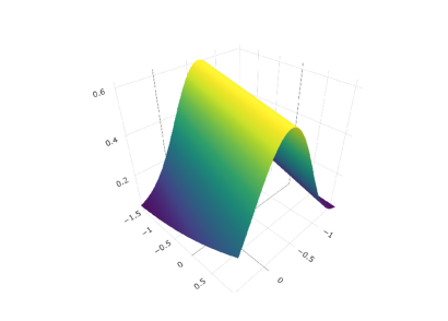
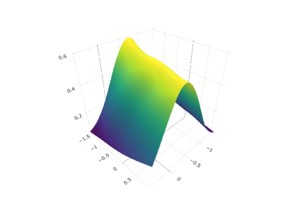
Figure 1. True transition density (left) and its estimation (right) for Model 1 ($N=200$ copies). Selected bandwidths: $\widehat{h}=0.22$ and $\widehat{\ell}=0.22$. 100*MISE = 0.253.

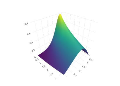
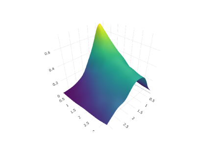
Figure 2. True transition density (left) and its estimation (right) for Model 3 ($N=200$ copies). Selected bandwidths: $\widehat{h}=0.18$ and $\widehat{\ell}=0.18$. 100*MISE = 0.315.

Model		$N=100$	$N=400$	$N=1000$
1	MISE	$0.979_{(0.535)}$	$0.244_{(0.129)}$	$0.140_{(0.107)}$
	Medians	0.880	0.223	0.107
	Mean of $\widehat{h}$	0.275	0.180	0.120
	Mean of $\widehat{\ell}$	0.288	0.165	0.140
2	MISE	$0.479_{(0.191)}$	$0.116_{(0.057)}$	$0.055_{(0.030)}$
	Medians	0.458	0.102	0.048
	Mean of $\widehat{h}$	0.098	0.06	0.042
	Mean of $\widehat{\ell}$	0.097	0.06	0.04
3	MISE	$1.052_{(2.374)}$	$0.343_{(0.506)}$	$0.177_{(0.414)}$
	Medians	0.771	0.243	0.102
	Mean of $\widehat{h}$	0.251	0.127	0.164
	Mean of $\widehat{\ell}$	0.262	0.107	0.1468

Table 1. First line: 100*MISE (with 100*StD) computed over 200 repetitions. Second line: median errors. Third (resp. fourth) line: mean of $\widehat{h}$ (resp. $\widehat{\ell}$).

Appendix A Proofs

A.1. Proof of Proposition 3.1

Consider $t\in(0,T]$. First of all,

$$\mathbb{E}(\|\widehat{s}_{\mathbf{h},t}-s_{t}\|^{2})=\int_{\mathbb{R}^{2}}\mathfrak{b}(x,y)^{2}dxdy+\int_{\mathbb{R}^{2}}\mathfrak{v}(x,y)dxdy$$

where, for any $(x,y)\in\mathbb{R}^{2}$,

$$\mathfrak{b}(x,y):=\mathbb{E}(\widehat{s}_{\mathbf{h},t}(x,y))-s_{t}(x,y)\quad{\rm and}\quad\mathfrak{v}(x,y):={\rm var}(\widehat{s}_{\mathbf{h},t}(x,y)).$$

First, let us find a suitable bound on the integrated squared-bias of $\widehat{s}_{\mathbf{h},t}$. Since $X^{1},\dots,X^{N}$ are i.i.d. copies of $X$, and by Equality (10),

$$\mathfrak{b}(x,y)+s_{t}(x,y) = \frac{1}{T-t_{0}}\int_{t_{0}}^{T}\mathbb{E}(Q_{\bf h}(X_{s}-x,X_{s+t}-y))ds$$

$$= \int_{\mathbb{R}^{2}}Q_{\bf h}(\xi-x,\zeta-y)$$

$$\hskip 56.9055pt\times\underbrace{\frac{1}{T-t_{0}}\int_{t_{0}}^{T}p_{s,s+t}(\xi,\eta)ds}_{=p_{t}(\xi,\zeta)f(\xi)}d\xi d\zeta$$

$$= \int_{\mathbb{R}^{2}}Q_{\bf h}(\xi-x,\zeta-y)s_{t}(\xi,\zeta)d\xi d\zeta=(Q_{\bf h}\star s_{t})(x,y).$$

Thus,

$$\int_{\mathbb{R}^{2}}\mathfrak{b}(x,y)^{2}dxdy=\|s_{\mathbf{h},t}-s_{t}\|^{2}.$$

Now, let us find a suitable bound on the integrated variance of $\widehat{s}_{\mathbf{h},t}$. Again, since $X^{1},\dots,X^{N}$ are i.i.d. copies of $X$, by Cauchy-Schwarz’s (or Jensen’s) inequality,

$$\mathfrak{v}(x,y) = \frac{1}{N(T-t_{0})^{2}}{\rm var}\left(\int_{t_{0}}^{T}Q_{\bf h}(X_{s}-x,X_{s+t}-y)ds\right)$$

$$\leqslant \frac{1}{N(T-t_{0})}\int_{t_{0}}^{T}\mathbb{E}(Q_{\bf h}(X_{s}-x,X_{s+t}-y)^{2})ds$$

$$= \frac{1}{N(T-t_{0})}\int_{t_{0}}^{T}\left[\frac{1}{h_{1}^{2}h_{2}^{2}}\int_{\mathbb{R}^{2}}K\left(\frac{\xi-x}{h_{1}}\right)^{2}K\left(\frac{\zeta-y}{h_{2}}\right)^{2}p_{s,s+t}(\xi,\zeta)d\xi d\zeta\right]ds.$$

Thus, by the Fubini-Tonelli theorem and the change of variable formula,

$$\int_{\mathbb{R}^{2}}\mathfrak{v}(x,y)dxdy = \frac{1}{N(T-t_{0})h_{1}^{2}h_{2}^{2}}\int_{\mathbb{R}^{2}}\left[\int_{\mathbb{R}^{2}}K\left(\frac{\xi-x}{h_{1}}\right)^{2}K\left(\frac{\zeta-y}{h_{2}}\right)^{2}dxdy\right]$$

$$\hskip 170.71652pt\times\left(\int_{t_{0}}^{T}p_{s,s+t}(\xi,\zeta)ds\right)d\xi d\zeta$$

$$= \frac{\|K\|^{4}}{N(T-t_{0})h_{1}h_{2}}\int_{\mathbb{R}^{2}}\left(\int_{t_{0}}^{T}p_{s,s+t}(\xi,\zeta)ds\right)d\xi d\zeta=\frac{\|K\|^{4}}{Nh_{1}h_{2}}.$$

Therefore,

$$\mathbb{E}(\|\widehat{s}_{\mathbf{h},t}-s_{t}\|^{2})\leqslant\|s_{\mathbf{h},t}-s_{t}\|^{2}+\frac{\|K\|^{4}}{Nh_{1}h_{2}}$$

and, by Inequality (6),

$$\mathbb{E}(\|\widehat{s}_{\mathbf{h},t}-s_{t}\|_{1\otimes f}^{2}) = \int_{\mathbb{R}^{2}}\mathfrak{b}(x,y)^{2}f(y)dxdy+\int_{\mathbb{R}^{2}}\mathfrak{v}(x,y)f(y)dxdy$$

$$\leqslant \|s_{\mathbf{h},t}-s_{t}\|_{1\otimes f}^{2}+2\mathfrak{c}_{T}(T-t_{0})^{-\frac{1}{2}}\frac{\|K\|^{4}}{Nh_{1}h_{2}}.$$

This concludes the proof.

A.2. Proof of Proposition 3.2

The proof of Proposition 3.2 relies on the following technical lemma.

Lemma A.1.

Let $\delta:\mathbb{R}\rightarrow\mathbb{R}_{+}$ be a density function. Under the conditions of Proposition 3.2, there exist two positive constants $\mathfrak{c}_{\ref{Nikolskii_type_condition}}$ and $p$, not depending on $t_{0}$, such that for every $t\in[t_{0},T]$ and $\theta\in\mathbb{R}$,

$$\int_{-\infty}^{\infty}\|p_{t}(\cdot,y+\theta)-p_{t}(\cdot,y)\|_{\delta}^{2}dy\leqslant\frac{\mathfrak{c}_{\ref{Nikolskii_type_condition}}}{t_{0}^{p}}(\theta^{2}+|\theta|^{3})$$

$$\hskip 85.35826pt\textrm{and}\quad\int_{-\infty}^{\infty}\|p_{t}(x+\theta,\cdot)-p_{t}(x,\cdot)\|_{\delta}^{2}dx\leqslant\frac{\mathfrak{c}_{\ref{Nikolskii_type_condition}}}{t_{0}^{p}}(\theta^{2}+|\theta|^{3}).$$

The proof of Lemma A.1 is postponed to Section A.2.1.

First, by the change of variable formula and the generalized Minkowski inequality (see Comte [2], Theorem B.1),

$$\|s_{\mathbf{h},t}-s_{t}\|_{1\otimes f}^{2} = \int_{\mathbb{R}^{2}}\left(\int_{\mathbb{R}^{2}}K(\xi)K(\zeta)(s_{t}(h_{1}\xi+x,h_{2}\zeta+y)-s_{t}(x,y))d\xi d\zeta\right)^{2}f(y)dxdy$$

$$\leqslant [\int_{\mathbb{R}^{2}}|K(\xi)K(\zeta)|$$

$$\hskip 28.45274pt\times\left(\int_{\mathbb{R}^{2}}(p_{t}(h_{1}\xi+x,h_{2}\zeta+y)f(h_{1}\xi+x)-p_{t}(x,y)f(x))^{2}f(y)dxdy\right)^{\frac{1}{2}}d\xi d\zeta]^{2}$$

$$\leqslant 3\left(\int_{\mathbb{R}^{2}}|K(\xi)K(\zeta)|(\mathfrak{b}_{1}(\xi,\zeta)+\mathfrak{b}_{2}(\xi,\zeta)+\mathfrak{b}_{3}(\xi,\zeta))^{\frac{1}{2}}d\xi d\zeta\right)^{2}$$

where, for any $(\xi,\zeta)\in\mathbb{R}^{2}$,

$$\mathfrak{b}_{1}(\xi,\zeta):=\int_{\mathbb{R}^{2}}f(y)p_{t}(h_{1}\xi+x,h_{2}\zeta+y)^{2}(f(h_{1}\xi+x)-f(x))^{2}dxdy,$$

$$\hskip 56.9055pt\mathfrak{b}_{2}(\xi,\zeta):=\int_{\mathbb{R}^{2}}f(y)f(x)^{2}(p_{t}(h_{1}\xi+x,h_{2}\zeta+y)-p_{t}(x,h_{2}\zeta+y))^{2}dxdy\quad{\rm and}$$

$$\hskip 113.81102pt\mathfrak{b}_{3}(\xi,\zeta):=\int_{\mathbb{R}^{2}}f(y)f(x)^{2}(p_{t}(x,h_{2}\zeta+y)-p_{t}(x,y))^{2}dxdy.$$

Now, let us find suitable bounds on $\mathfrak{b}_{1}(\xi,\zeta)$, $\mathfrak{b}_{2}(\xi,\zeta)$ and $\mathfrak{b}_{3}(\xi,\zeta)$.

• Bound on $\mathfrak{b}_{1}(\xi,\zeta)$. By Kusuoka and Stroock [13], Corollary 3.25, there exist two positive constants $\mathfrak{c}_{1}$ and $\mathfrak{m}_{1}$ such that, for every $t\in(0,T]$ and $(x,y)\in\mathbb{R}^{2}$,

  (17) $$0<p_{t}(x,y)\leqslant\frac{\mathfrak{c}_{1}}{\sqrt{t}}\exp\left[-\mathfrak{m}_{1}\frac{(y-x)^{2}}{t}\right].$$

  Then, by Inequalities (6) and (17), and since $T-t_{0}\geqslant 1$, for any $(\xi,\zeta)\in\mathbb{R}^{2}$,

  $$\int_{-\infty}^{\infty}f(y)p_{t}(h_{1}\xi+x,h_{2}\zeta+y)^{2}dy \leqslant \|f\|_{\infty}\frac{\mathfrak{c}_{1}^{2}}{t}\int_{-\infty}^{\infty}\exp\left[-2\mathfrak{m}_{1}\frac{(h_{2}\zeta+y-h_{1}\xi-x)^{2}}{t}\right]dy$$

  $$\leqslant \frac{2\mathfrak{c}_{1}^{3}}{t}\int_{-\infty}^{\infty}\exp\left(-2\mathfrak{m}_{1}\frac{y^{2}}{t}\right)dy$$

  $$\leqslant \frac{\mathfrak{c}_{2}}{t_{0}}\quad{\rm with}\quad\mathfrak{c}_{2}=2\mathfrak{c}_{1}^{3}\int_{-\infty}^{\infty}\exp\left(-2\mathfrak{m}_{1}\frac{y^{2}}{T}\right)dy.$$

  So, by Marie and Rosier [19], Corollary 1,

  $$\mathfrak{b}_{1}(\xi,\zeta)\leqslant\frac{\mathfrak{c}_{2}}{t_{0}}\int_{-\infty}^{\infty}(f(h_{1}\xi+x)-f(x))^{2}dx\\ \leqslant\frac{\mathfrak{c}_{3}}{t_{0}^{q+1}}h_{1}^{2}(\xi^{2}+|\xi|^{3}),$$

  where $\mathfrak{c}_{3}$ and $q$ are positive constants not depending on $t_{0}$, $h_{1}$ and $\xi$.

• Bounds on $\mathfrak{b}_{2}(\xi,\zeta)$ and $\mathfrak{b}_{3}(\xi,\zeta)$. By Lemma A.1 and Inequality (6),

  $$\mathfrak{b}_{2}(\xi,\zeta)+\mathfrak{b}_{3}(\xi,\zeta) \leqslant \|f\|_{\infty}^{2}\int_{\mathbb{R}^{2}}f(y-h_{2}\zeta)(p_{t}(h_{1}\xi+x,y)-p_{t}(x,y))^{2}dxdy$$

  $$\hskip 56.9055pt+\|f\|_{\infty}^{2}\int_{\mathbb{R}^{2}}f(x)(p_{t}(x,h_{2}\zeta+y)-p_{t}(x,y))^{2}dxdy$$

  $$\leqslant \frac{\mathfrak{c}_{4}}{t_{0}^{p}}(h_{1}^{2}(\xi^{2}+|\xi|^{3})+h_{2}^{2}(\zeta^{2}+|\zeta|^{3})),$$

  where $\mathfrak{c}_{4}$ and $p$ are positive constants not depending on $t_{0}$, $\mathbf{h}$, $\xi$ and $\zeta$.

Thus, by the conditions on the kernel function $K$,

$$\|s_{\mathbf{h},t}-s_{t}\|_{1\otimes f}^{2} \leqslant \frac{\mathfrak{c}_{3}\vee\mathfrak{c}_{4}}{t_{0}^{q+1}\wedge t_{0}^{p}}\left(2h_{1}\int_{\mathbb{R}^{2}}|K(\xi)K(\zeta)|(\xi^{2}+|\xi|^{3})^{\frac{1}{2}}d\xi d\zeta\right.$$

$$\hskip 113.81102pt\left.+h_{2}\int_{\mathbb{R}^{2}}|K(\xi)K(\zeta)|(\zeta^{2}+|\zeta|^{3})^{\frac{1}{2}}d\xi d\zeta\right)^{2}$$

$$\leqslant \frac{2(\mathfrak{c}_{3}\vee\mathfrak{c}_{4})}{(1\wedge t_{0})^{p+q+1}}(4h_{1}^{2}+h_{2}^{2})\|K\|_{1}^{2}\underbrace{\left(\int_{-\infty}^{\infty}|K(\xi)|(\xi^{2}+|\xi|^{3})^{\frac{1}{2}}d\xi\right)^{2}}_{<\infty}$$

$$\leqslant \frac{\mathfrak{c}_{5}}{(1\wedge t_{0})^{p+q+1}}(h_{1}^{2}+h_{2}^{2}),$$

where $\mathfrak{c}_{5}$ is a positive constant not depending on $t_{0}$ and $\mathbf{h}$. This concludes the proof.

A.2.1. Proof of Lemma A.1

The proof of Lemma A.1 is similar to that of Marie and Rosier [19], Corollary 1. By Kusuoka and Stroock [13], Corollary 3.25, there exist three positive constants $\mathfrak{c}_{1}$, $\mathfrak{m}_{1}$ and $q$ such that, for every $t\in(0,T]$ and $(x,y)\in\mathbb{R}^{2}$,

(18) $$|\partial_{1}p_{t}(x,y)|+|\partial_{2}p_{t}(x,y)|\leqslant\frac{\mathfrak{c}_{1}}{t^{q}}\exp\left[-\mathfrak{m}_{1}\frac{(y-x)^{2}}{t}\right].$$

For any $t\in[t_{0},T]$ and $\vartheta\in\mathbb{R}_{+}$, by Inequality (18),

$$\int_{-\infty}^{\infty}\|p_{t}(\cdot,y+\vartheta)-p_{t}(\cdot,y)\|_{\delta}^{2}dy \leqslant \vartheta^{2}\int_{-\infty}^{\infty}\delta(x)\int_{-\infty}^{\infty}\left(\sup_{z\in[y,y+\vartheta]}|\partial_{2}p_{t}(x,x+z)|^{2}\right)dydx$$

$$\leqslant \vartheta^{2}\frac{\mathfrak{c}_{1}^{2}}{t^{2q}}\left(\int_{-\infty}^{\infty}\delta(x)dx\right)\int_{-\infty}^{\infty}\left[\sup_{z\in[y,y+\vartheta]}\exp\left(-2\mathfrak{m}_{1}\frac{z^{2}}{t}\right)\right]dy$$

$$= \vartheta^{2}\frac{\mathfrak{c}_{1}^{2}}{t^{2q}}\left[\int_{-\infty}^{-\vartheta}\exp\left(-2\mathfrak{m}_{1}\frac{(y+\vartheta)^{2}}{t}\right)dy+\vartheta+\int_{0}^{\infty}\exp\left(-2\mathfrak{m}_{1}\frac{y^{2}}{t}\right)dy\right]$$

$$\leqslant \frac{\mathfrak{c}_{1}^{2}}{t_{0}^{2q}}(\mathfrak{c}_{2}\vartheta^{2}+\vartheta^{3})$$

with

$$\mathfrak{c}_{2}=2\int_{0}^{\infty}\exp\left(-2\mathfrak{m}_{1}\frac{y^{2}}{T}\right)dy,$$

and the same way,

$$\int_{-\infty}^{\infty}\|p_{t}(\cdot,y-\vartheta)-p_{t}(\cdot,y)\|_{\delta}^{2}dy \leqslant \vartheta^{2}\frac{\mathfrak{c}_{1}^{2}}{t^{2q}}\left(\int_{-\infty}^{0}\exp\left(-2\mathfrak{m}_{1}\frac{y^{2}}{t}\right)dy+\vartheta+\int_{\vartheta}^{\infty}\exp\left(-2\mathfrak{m}_{1}\frac{(y-\vartheta)^{2}}{t}\right)dy\right)$$

$$\leqslant \frac{\mathfrak{c}_{1}^{2}}{t_{0}^{2q}}(\mathfrak{c}_{2}\vartheta^{2}+\vartheta^{3}).$$

Thus, for any $\theta\in\mathbb{R}$,

$$\int_{-\infty}^{\infty}\|p_{t}(\cdot,y+\theta)-p_{t}(\cdot,y)\|_{\delta}^{2}dy\leqslant\frac{\mathfrak{c}_{1}^{2}}{t_{0}^{2q}}(\mathfrak{c}_{2}\theta^{2}+|\theta|^{3}).$$

By following the same line, Inequality (18) leads to

$$\int_{-\infty}^{\infty}\|p_{t}(x+\theta,\cdot)-p_{t}(x,\cdot)\|_{\delta}^{2}dx\leqslant\frac{\mathfrak{c}_{1}^{2}}{t_{0}^{2q}}(\mathfrak{c}_{2}\theta^{2}+|\theta|^{3}).$$

This concludes the proof.

A.3. Proof of Corollary 3.3

First of all, for any $t\in(0,T]$,

$$\widehat{p}_{\mathbf{h},\ell,t}-p_{t}=\left[\frac{\widehat{s}_{\mathbf{h},t}-s_{t}}{\widehat{f}_{\ell}}+\left(\frac{1}{\widehat{f}_{\ell}}-\frac{1}{f}\right)p_{t}f\right]\mathbf{1}_{\widehat{f}_{\ell}(\cdot)>\frac{m}{2}}-p_{t}\mathbf{1}_{\widehat{f}_{\ell}(\cdot)\leqslant\frac{m}{2}}.$$

Then,

$$\|\widehat{p}_{\mathbf{h},\ell,t}-p_{t}\|_{[\texttt{l},\texttt{r}]\times\mathbb{R}}^{2}=\left\|\left[\frac{\widehat{s}_{\mathbf{h},t}-s_{t}}{\widehat{f}_{\ell}}+\left(\frac{1}{\widehat{f}_{\ell}}-\frac{1}{f}\right)p_{t}f\right]\mathbf{1}_{\widehat{f}_{\ell}(\cdot)>\frac{m}{2}}\right\|_{[\texttt{l},\texttt{r}]\times\mathbb{R}}^{2}+\|p_{t}\mathbf{1}_{\widehat{f}_{\ell}(\cdot)\leqslant\frac{m}{2}}\|_{[\texttt{l},\texttt{r}]\times\mathbb{R}}^{2}.$$

Moreover, for any $x\in[\texttt{l},\texttt{r}]$, since $f(x)>m$, for every $\omega\in\{\widehat{f}_{\ell}(\cdot)\leqslant m/2\}$,

$$|f(x)-\widehat{f}_{\ell}(x,\omega)|\geqslant f(x)-\widehat{f}_{\ell}(x,\omega)>m-\frac{m}{2}=\frac{m}{2}.$$

Thus,

$$\|\widehat{p}_{\mathbf{h},\ell,t}-p_{t}\|_{[\texttt{l},\texttt{r}]\times\mathbb{R}}^{2} \leqslant \frac{8}{m^{2}}\|\widehat{s}_{\mathbf{h},t}-s_{t}\|_{[\texttt{l},\texttt{r}]\times\mathbb{R}}^{2}+\frac{8}{m^{2}}\|(f-\widehat{f}_{\ell})p_{t}\|_{[\texttt{l},\texttt{r}]\times\mathbb{R}}^{2}+2\|p_{t}\mathbf{1}_{|f(\cdot)-\widehat{f}_{\ell}(\cdot)|>\frac{m}{2}}\|_{[\texttt{l},\texttt{r}]\times\mathbb{R}}^{2}$$

$$\leqslant \frac{8}{m^{2}}\int_{[\texttt{l},\texttt{r}]\times\mathbb{R}}(\widehat{s}_{\mathbf{h},t}-s_{t})(x,y)^{2}dxdy$$

$$\hskip 28.45274pt+\frac{8}{m^{2}}\int_{[\texttt{l},\texttt{r}]\times\mathbb{R}}(f(x)-\widehat{f}_{\ell}(x))^{2}p_{t}(x,y)^{2}dxdy$$

$$\hskip 56.9055pt+2\int_{[\texttt{l},\texttt{r}]\times\mathbb{R}}p_{t}(x,y)^{2}\mathbf{1}_{|f(x)-\widehat{f}_{\ell}(x)|>\frac{m}{2}}dxdy.$$

By Inequality (5), and since $p_{t}(x,\cdot)$ ($x\in\mathbb{R}$) is a density function,

$$\|\widehat{p}_{\mathbf{h},\ell,t}-p_{t}\|_{[\texttt{l},\texttt{r}]\times\mathbb{R}}^{2}\leqslant\frac{8}{m^{2}}\|\widehat{s}_{\mathbf{h},t}-s_{t}\|_{[\texttt{l},\texttt{r}]\times\mathbb{R}}^{2}+\frac{8}{m^{2}}\mathfrak{m}_{p}(t_{0},T)\|\widehat{f}_{\ell}-f\|^{2}+2\mathfrak{m}_{p}(t_{0},T)\int_{-\infty}^{\infty}\mathbf{1}_{|f(x)-\widehat{f}_{\ell}(x)|>\frac{m}{2}}dx.$$

Therefore, by Markov’s inequality,

(19) $$\mathbb{E}(\|\widehat{p}_{\mathbf{h},\ell,t}-p_{t}\|_{[\texttt{l},\texttt{r}]\times\mathbb{R}}^{2}) \leqslant \frac{8}{m^{2}}\mathbb{E}(\|\widehat{s}_{\mathbf{h},t}-s_{t}\|_{[\texttt{l},\texttt{r}]\times\mathbb{R}}^{2})+\frac{8}{m^{2}}\mathfrak{m}_{p}(t_{0},T)\mathbb{E}(\|\widehat{f}_{\ell}-f\|^{2})$$

$$\hskip 128.0374pt+\frac{8}{m^{2}}\mathfrak{m}_{p}(t_{0},T)\int_{-\infty}^{\infty}\mathbb{E}((f(x)-\widehat{f}_{\ell}(x))^{2})dx$$

$$\leqslant \frac{8}{m^{2}}\max\{1,\mathfrak{m}_{p}(t_{0},T)\}(\mathbb{E}(\|\widehat{s}_{\mathbf{h},t}-s_{t}\|_{[\texttt{l},\texttt{r}]\times\mathbb{R}}^{2})+2\mathbb{E}(\|\widehat{f}_{\ell}-f\|^{2})),$$

leading to Inequality (11) thanks to Proposition 3.1 and Marie and Rosier [19], Proposition 1. By Inequality (6), and since $f(\cdot)>m$ on $[\texttt{l},\texttt{r}]$,

$$m\|.\|_{[\texttt{l},\texttt{r}]\times\mathbb{R}}^{2}\leqslant\|.\|_{1\otimes f,[\texttt{l},\texttt{r}]\times\mathbb{R}}^{2}\leqslant\mathfrak{m}_{f}(t_{0},T)\|.\|_{[\texttt{l},\texttt{r}]\times\mathbb{R}}^{2},$$

and then one may also establish Inequality (3.3) thanks to Inequality (19).

A.4. Proof of Theorem 4.1

For any $t\in[t_{0},T]$ and $\mathbf{h}\in(0,1]^{2}$, consider the map $\Phi_{\mathbf{h},t}$ defined on $C^{0}([0,T])\times\mathbb{R}^{2}$ by

$$\Phi_{\mathbf{h},t}(\varphi;x,y):=\frac{1}{T-t_{0}}\int_{t_{0}}^{T}Q_{\bf h}(\varphi(s)-x,\varphi(s+t)-y)ds$$

for every $\varphi\in C^{0}([0,T])$ and $(x,y)\in\mathbb{R}^{2}$. Then,

$$\widehat{s}_{\mathbf{h},t}(\cdot)=\frac{1}{N}\sum_{i=1}^{N}\Phi_{\mathbf{h},t}(X^{i};\cdot).$$

First, the following proposition shows that

$$\mathcal{K}_{N}:=\{(\varphi,x,y)\mapsto\Phi_{\mathbf{h},t}(\varphi;x,y)\textrm{ $;$ }\mathbf{h}\in\mathcal{H}_{N}^{2}\}$$

satisfies properties close to those of a kernels set in the nonparametric regression framework (see Halconruy and Marie [11], Assumption 2.1).

Proposition A.2.

Under the conditions of Theorem 4.1, there exists a constant $\mathfrak{m}_{\Phi}>0$, not depending on $t$, such that:

1. For every $\mathbf{h}=(h_{1},h_{2})\in(0,1]^{2}$ and $\varphi\in C^{0}([0,T])$,

   $$\|\Phi_{\mathbf{h},t}(\varphi;\cdot)\|^{2}\leqslant\frac{\mathfrak{m}_{\Phi}}{h_{1}h_{2}}.$$

2. For every $\mathbf{h},\mathbf{l}\in(0,1]^{2}$,

   $$\mathbb{E}(\langle\Phi_{\mathbf{h},t}(X^{1};\cdot),\Phi_{\mathbf{l},t}(X^{2};\cdot)\rangle^{2})\leqslant\mathfrak{m}_{\Phi}\overline{s}_{\mathbf{l},t},$$

   where

   $$\overline{s}_{\mathbf{l},t}:=\mathbb{E}(\|\Phi_{\mathbf{l},t}(X;\cdot)\|^{2}).$$

3. For every $\mathbf{h}\in(0,1]^{2}$ and $\varphi\in\mathbb{L}^{2}(\mathbb{R}^{2})$,

   $$\mathbb{E}(\langle\Phi_{\mathbf{h},t}(X;\cdot),\varphi\rangle^{2})\leqslant\mathfrak{m}_{\Phi}\|\varphi\|^{2}.$$

4. For every $\mathbf{h},\mathbf{l}\in(0,1]^{2}$,

   $$|\langle\Phi_{\mathbf{h},t}(X;\cdot),s_{\mathbf{l},t}\rangle|\leqslant\mathfrak{m}_{\Phi},$$

   where

   $$s_{\mathbf{l},t}(\cdot)=\mathbb{E}(\widehat{s}_{\mathbf{l},t}(\cdot))=(Q_{\bf l}\star s_{t})(\cdot).$$

The proof of Proposition A.2 is postponed to Section A.4.2. Now, the three following lemmas deal with controls of the maps $U$, $V$ and $W$ involved in the proof of Theorem 4.1 (see (the next) Section A.4.1).

Lemma A.3.

For every $\mathbf{h},\mathbf{l}\in\mathcal{H}_{N}^{2}$, consider

$$U_{\mathbf{h},\mathbf{l}}:=\sum_{i\neq k}\langle\Phi_{\mathbf{h},t}(X^{i};\cdot)-s_{\mathbf{h},t},\Phi_{\mathbf{l},t}(X^{k};\cdot)-s_{\mathbf{l},t}\rangle.$$

There exists a deterministic constant $\mathfrak{c}_{\ref{control_U_term}}>0$, not depending on $N$ and $t$, such that for every $\theta\in(0,1)$ and $\lambda>0$, with probability larger than $1-5.4|\mathcal{H}_{N}|^{2}e^{-\lambda}$,

$$\sup_{\mathbf{h}\in\mathcal{H}_{N}^{2}}\left\{\frac{|U_{\mathbf{h},\mathbf{h}_{0}}|}{N^{2}}-\frac{\theta}{N}\overline{s}_{\mathbf{h},t}\right\} \leqslant \frac{\mathfrak{c}_{\ref{control_U_term}}(1+\lambda)^{3}}{\theta N}$$

$$\textrm{and}\quad\sup_{\mathbf{h}\in\mathcal{H}_{N}^{2}}\left\{\frac{|U_{\mathbf{h},\mathbf{h}}|}{N^{2}}-\frac{\theta}{N}\overline{s}_{\mathbf{h},t}\right\}\leqslant\frac{\mathfrak{c}_{\ref{control_U_term}}(1+\lambda)^{3}}{\theta N}.$$

Lemma A.4.

For every $\mathbf{h}\in\mathcal{H}_{N}^{2}$, consider

$$V_{\bf h}:=\frac{1}{N}\sum_{i=1}^{N}\|\Phi_{\mathbf{h},t}(X^{i};\cdot)-s_{\mathbf{h},t}\|^{2}.$$

There exists a deterministic constant $\mathfrak{c}_{\ref{control_V_term}}>0$, not depending on $N$ and $t$, such that for every $\theta\in(0,1)$ and $\lambda>0$, with probability larger than $1-2|\mathcal{H}_{N}|^{2}e^{-\lambda}$,

$$\sup_{\mathbf{h}\in\mathcal{H}_{N}^{2}}\left\{\frac{1}{N}|V_{\bf h}-\overline{s}_{\mathbf{h},t}|-\frac{\theta}{N}\overline{s}_{\mathbf{h},t}\right\}\leqslant\frac{\mathfrak{c}_{\ref{control_V_term}}(1+\lambda)}{\theta N}.$$

Lemma A.5.

For every $\mathbf{h},\mathbf{l}\in\mathcal{H}_{N}^{2}$, consider

$$W_{\mathbf{h},\mathbf{l}}:=\langle\widehat{s}_{\mathbf{h},t}-s_{\mathbf{h},t},s_{\mathbf{l},t}-s_{t}\rangle.$$

There exists a deterministic constant $\mathfrak{c}_{\ref{control_W_term}}>0$, not depending on $N$ and $t$, such that for every $\theta\in(0,1)$ and $\lambda>0$, with probability larger than $1-2|\mathcal{H}_{N}|^{2}e^{-\lambda}$,

$$\sup_{\mathbf{h}\in\mathcal{H}_{N}^{2}}\{|W_{\mathbf{h},\mathbf{h}_{0}}|-\theta\|s_{\mathbf{h}_{0},t}-s_{t}\|^{2}\}\leqslant\frac{\mathfrak{c}_{\ref{control_W_term}}(1+\lambda)^{2}}{\theta N},$$

$$\hskip 56.9055pt\sup_{\mathbf{h}\in\mathcal{H}_{N}^{2}}\{|W_{\mathbf{h}_{0},\mathbf{h}}|-\theta\|s_{\mathbf{h},t}-s_{t}\|^{2}\}\leqslant\frac{\mathfrak{c}_{\ref{control_W_term}}(1+\lambda)^{2}}{\theta N}$$

$$\hskip 113.81102pt{\rm and}\quad\sup_{\mathbf{h}\in\mathcal{H}_{N}^{2}}\{|W_{\mathbf{h},\mathbf{h}}|-\theta\|s_{\mathbf{h},t}-s_{t}\|^{2}\}\leqslant\frac{\mathfrak{c}_{\ref{control_W_term}}(1+\lambda)^{2}}{\theta N}.$$

As in Marie and Rosier [19] (see [19], Lemmas 4, 5 and 6), the proofs of Lemmas A.3, A.4 and A.5 rely on Proposition A.2, on a concentration inequality for U-statistics (see Giné and Nickl [10], Theorem 3.4.8), and on the weak Bernstein inequality (see Massart [20], Proposition 2.9 and Inequality (2.23)). So, the proofs of Lemmas A.3, A.4 and A.5 are left to the reader.

A.4.1. Steps of the proof of Theorem 4.1

The proof of Theorem 4.1 is dissected in four steps. Step 1 shows that, for any $\mathbf{h}\in\mathcal{H}_{N}^{2}$,

$$\|\widehat{s}_{\widehat{\bf h},t}-s_{t}\|^{2}\leqslant\|\widehat{s}_{\mathbf{h},t}-s_{t}\|^{2}-\psi(\mathbf{h})+\psi(\widehat{\bf h}),$$

where $\psi$ is a map depending on $U$ and $W$. Then, $\psi(\mathbf{h})$ and $\psi(\widehat{\bf h})$ are controlled in Step 2 thanks to Lemmas A.3 and A.5. Step 3 deals with a two-sided relationship between

$$\|\widehat{s}_{\mathbf{h},t}-s_{t}\|^{2}\quad{\rm and}\quad\|s_{\mathbf{h},t}-s_{t}\|^{2}\textrm{ $;$ }\mathbf{h}\in\mathcal{H}_{N}^{2},$$

thanks to Lemmas A.3, A.4 and A.5. The conclusion comes in Step 4.

Step 1. First,

$$\|\widehat{s}_{\widehat{\bf h},t}-s_{t}\|^{2}=\|\widehat{s}_{\widehat{\bf h},t}-\widehat{s}_{\mathbf{h}_{0},t}\|^{2}+\|\widehat{s}_{\mathbf{h}_{0},t}-s_{t}\|^{2}+2\langle\widehat{s}_{\widehat{\bf h},t}-\widehat{s}_{\mathbf{h}_{0},t},\widehat{s}_{\mathbf{h}_{0},t}-s_{t}\rangle$$

and, for any $\mathbf{h}\in\mathcal{H}_{N}^{2}$,

$$\|\widehat{s}_{\widehat{\bf h},t}-\widehat{s}_{\mathbf{h}_{0},t}\|^{2} \leqslant \|\widehat{s}_{\mathbf{h},t}-\widehat{s}_{\mathbf{h}_{0},t}\|^{2}+{\rm pen}(\mathbf{h})-{\rm pen}(\widehat{\bf h})\quad\textrm{by (\ref{PCO_criterion_numerator})}$$

$$= \|\widehat{s}_{\mathbf{h},t}-s_{t}\|^{2}+2\langle\widehat{s}_{\mathbf{h},t}-s_{t},s_{t}-\widehat{s}_{\mathbf{h}_{0},t}\rangle+\|s_{t}-\widehat{s}_{\mathbf{h}_{0},t}\|^{2}+{\rm pen}(\mathbf{h})-{\rm pen}(\widehat{\bf h})$$

$$= \|\widehat{s}_{\mathbf{h},t}-s_{t}\|^{2}+2\langle\widehat{s}_{\mathbf{h},t}-\widehat{s}_{\mathbf{h}_{0},t},s_{t}-\widehat{s}_{\mathbf{h}_{0},t}\rangle-\|s_{t}-\widehat{s}_{\mathbf{h}_{0},t}\|^{2}+{\rm pen}(\mathbf{h})-{\rm pen}(\widehat{\bf h}).$$

Then,

(20) $$\|\widehat{s}_{\widehat{\bf h},t}-s_{t}\|^{2} \leqslant \|\widehat{s}_{\mathbf{h},t}-s_{t}\|^{2}+2\langle\widehat{s}_{\mathbf{h},t}-\widehat{s}_{\mathbf{h}_{0},t},s_{t}-\widehat{s}_{\mathbf{h}_{0},t}\rangle$$

$$\hskip 85.35826pt+{\rm pen}(\mathbf{h})-{\rm pen}(\widehat{\bf h})+2\langle\widehat{s}_{\widehat{\bf h},t}-\widehat{s}_{\mathbf{h}_{0},t},\widehat{s}_{\mathbf{h}_{0},t}-s_{t}\rangle$$

$$= \|\widehat{s}_{\mathbf{h},t}-s_{t}\|^{2}+{\rm pen}(\mathbf{h})-{\rm pen}(\widehat{\bf h})+2\langle\widehat{s}_{\widehat{\bf h},t}-\widehat{s}_{\mathbf{h},t},\widehat{s}_{\mathbf{h}_{0},t}-s_{t}\rangle$$

$$= \|\widehat{s}_{\mathbf{h},t}-s_{t}\|^{2}-\psi(\mathbf{h})+\psi(\widehat{\bf h}),$$

where

$$\psi(\cdot):=2\langle\widehat{s}_{.,t}-s_{t},\widehat{s}_{\mathbf{h}_{0},t}-s_{t}\rangle-\textrm{pen}(\cdot).$$

Now, let us rewrite $\psi(\cdot)$ in terms of $U_{.,\mathbf{h}_{0}}$, $W_{.,\mathbf{h}_{0}}$ and $W_{\mathbf{h}_{0},.}$. For any $\mathbf{h}\in\mathcal{H}_{N}^{2}$,

$$\psi(\mathbf{h}) = 2\langle\widehat{s}_{\mathbf{h},t}-s_{\mathbf{h},t}+s_{\mathbf{h},t}-s_{t},\widehat{s}_{\mathbf{h}_{0},t}-s_{\mathbf{h}_{0},t}+s_{\mathbf{h}_{0},t}-s_{t}\rangle-{\rm pen}(\mathbf{h})$$

$$= 2\langle\widehat{s}_{\mathbf{h},t}-s_{\mathbf{h},t},\widehat{s}_{\mathbf{h}_{0},t}-s_{\mathbf{h}_{0},t}\rangle-{\rm pen}(\mathbf{h})$$

$$\hskip 71.13188pt+2\underbrace{(W_{\mathbf{h},\mathbf{h}_{0}}+W_{\mathbf{h}_{0},\mathbf{h}}+\langle s_{\mathbf{h},t}-s_{t},s_{\mathbf{h}_{0},t}-s_{t}\rangle)}_{=:\psi_{3}(\mathbf{h})}$$

$$= \frac{2U_{\mathbf{h},\mathbf{h}_{0}}}{N^{2}}+2\underbrace{\left(\frac{1}{N^{2}}\sum_{i=1}^{N}\langle\Phi_{\mathbf{h},t}(X^{i};\cdot)-s_{\mathbf{h},t},\Phi_{\mathbf{h}_{0},t}(X^{i};\cdot)-s_{\mathbf{h}_{0},t}\rangle-\frac{{\rm pen}(\mathbf{h})}{2}\right)}_{=:\psi_{2}(\mathbf{h})}+2\psi_{3}(\mathbf{h})$$

and, by the definition of ${\rm pen}(\mathbf{h})$,

$$\psi_{2}(\mathbf{h})=-\frac{1}{N^{2}}\left(\sum_{i=1}^{N}\langle\Phi_{\mathbf{h},t}(X^{i};\cdot),s_{\mathbf{h}_{0},t}\rangle+\sum_{i=1}^{N}\langle\Phi_{\mathbf{h}_{0},t}(X^{i};\cdot),s_{\mathbf{h},t}\rangle\right)+\frac{1}{N}\langle s_{\mathbf{h},t},s_{\mathbf{h}_{0},t}\rangle.$$

So,

$$\psi(\mathbf{h})=2(\psi_{1}(\mathbf{h})+\psi_{2}(\mathbf{h})+\psi_{3}(\mathbf{h}))\quad{\rm with}\quad\psi_{1}(\mathbf{h})=\frac{U_{\mathbf{h},\mathbf{h}_{0}}}{N^{2}}.$$

Step 2. This step deals with suitable bounds on the $\psi_{j}$’s.

• Consider $\mathbf{h}\in\mathcal{H}_{N}$. By Lemma A.3, for any $\lambda>0$ and $\theta\in(0,1)$, with probability larger than $1-5.4|\mathcal{H}_{N}|^{2}e^{-\lambda}$,

  $$|\psi_{1}(\mathbf{h})| \leqslant \frac{\theta}{2N}\overline{s}_{\mathbf{h},t}+\frac{2\mathfrak{c}_{\ref{control_U_term}}(1+\lambda)^{3}}{\theta N}$$

  $$\hskip 42.67912pt{\rm and}\quad|\psi_{1}(\widehat{\bf h})|\leqslant\frac{\theta}{2N}\overline{s}_{\widehat{\bf h},t}+\frac{2\mathfrak{c}_{\ref{control_U_term}}(1+\lambda)^{3}}{\theta N}.$$

• For any $\mathbf{h},\mathbf{l}\in\mathcal{H}_{N}^{2}$, consider

  $$\overline{\psi}_{2}(\mathbf{h},\mathbf{l}):=\frac{1}{N}\sum_{i=1}^{N}\langle\Phi_{\mathbf{h},t}(X^{i};\cdot),s_{\mathbf{l},t}\rangle.$$

  By Proposition A.2.(4),

  $$|\overline{\psi}_{2}(\mathbf{h},\mathbf{l})|\leqslant\mathfrak{m}_{\Phi}.$$

  Moreover, since $s_{t}\in\mathbb{L}^{2}(\mathbb{R}^{2})$ by Inequality (7),

  $$|\langle s_{\mathbf{h},t},s_{\mathbf{h}_{0},t}\rangle|\leqslant\|Q_{\bf h}\star s_{t}\|\cdot\|Q_{\mathbf{h}_{0}}\star s_{t}\|\leqslant\|K\|_{1}^{4}\|s_{t}\|^{2}.$$

  Then, there exists a deterministic constant $\mathfrak{c}_{1}>0$, not depending on $N$ and $t$, such that

  $$|\psi_{2}(\mathbf{h})|\vee|\psi_{2}(\widehat{\bf h})|\leqslant\sup_{\mathbf{l}\in\mathcal{H}_{N}^{2}}|\psi_{2}(\mathbf{l})|\leqslant\frac{\mathfrak{c}_{1}}{N}.$$

• Consider $\mathbf{h}\in\mathcal{H}_{N}^{2}$. By Lemma A.5 and Cauchy-Schwarz’s inequality, with probability larger than $1-|\mathcal{H}_{N}|^{2}e^{-\lambda}$,

  $$|\psi_{3}(\mathbf{h})| \leqslant \frac{\theta}{4}(\|s_{\mathbf{h},t}-s_{t}\|^{2}+\|s_{\mathbf{h}_{0},t}-s_{t}\|^{2})+\frac{8\mathfrak{c}_{\ref{control_W_term}}(1+\lambda)^{2}}{\theta N}$$

  $$\hskip 42.67912pt+2\left(\frac{1}{2}\right)^{\frac{1}{2}}\left(\frac{\theta}{2}\right)^{\frac{1}{2}}\|s_{\mathbf{h},t}-s_{t}\|\times\left(\frac{1}{2}\right)^{\frac{1}{2}}\left(\frac{2}{\theta}\right)^{\frac{1}{2}}\|s_{\mathbf{h}_{0},t}-s_{t}\|$$

  $$\leqslant \frac{\theta}{2}\|s_{\mathbf{h},t}-s_{t}\|^{2}+\left(\frac{\theta}{4}+\frac{1}{\theta}\right)\|s_{\mathbf{h}_{0},t}-s_{t}\|^{2}+\frac{8\mathfrak{c}_{\ref{control_W_term}}(1+\lambda)^{2}}{\theta N}$$

  and

  $$|\psi_{3}(\widehat{\bf h})|\leqslant\frac{\theta}{2}\|s_{\widehat{\bf h},t}-s_{t}\|^{2}+\left(\frac{\theta}{4}+\frac{1}{\theta}\right)\|s_{\mathbf{h}_{0},t}-s_{t}\|^{2}+\frac{8\mathfrak{c}_{\ref{control_W_term}}(1+\lambda)^{2}}{\theta N}.$$

Step 3. Let us establish that there exist two deterministic constants $\mathfrak{c}_{2},\overline{\mathfrak{c}}_{2}>0$, not depending on $N$, $t$ and $\theta$, such that with probability larger than $1-\overline{\mathfrak{c}}_{2}|\mathcal{H}_{N}|^{2}e^{-\lambda}$,

$$\sup_{\mathbf{h}\in\mathcal{H}_{N}^{2}}\left\{\|\widehat{s}_{\mathbf{h},t}-s_{t}\|^{2}-(1+\theta)\left(\|s_{\mathbf{h},t}-s_{t}\|^{2}+\frac{\overline{s}_{\mathbf{h},t}}{N}\right)\right\}\leqslant\frac{\mathfrak{c}_{2}(1+\lambda)^{3}}{\theta N}$$

and

$$\sup_{\mathbf{h}\in\mathcal{H}_{N}^{2}}\left\{\|s_{\mathbf{h},t}-s_{t}\|^{2}+\frac{\overline{s}_{\mathbf{h},t}}{N}-\frac{1}{1-\theta}\|\widehat{s}_{\mathbf{h},t}-s_{t}\|^{2}\right\}\leqslant\frac{\mathfrak{c}_{2}(1+\lambda)^{3}}{\theta(1-\theta)N}.$$

On the one hand, for any $\mathbf{h}\in\mathcal{H}_{N}^{2}$,

$$\|\widehat{s}_{\mathbf{h},t}-s_{t}\|^{2}-(1+\theta)\left(\|s_{\mathbf{h},t}-s_{t}\|^{2}+\frac{\overline{s}_{\mathbf{h},t}}{N}\right)$$

$$\hskip 56.9055pt=\|\widehat{s}_{\mathbf{h},t}-s_{\mathbf{h},t}\|^{2}+2\langle\widehat{s}_{\mathbf{h},t}-s_{\mathbf{h},t},s_{\mathbf{h},t}-s_{t}\rangle+\|s_{\mathbf{h},t}-s_{t}\|^{2}-(1+\theta)\left(\|s_{\mathbf{h},t}-s_{t}\|^{2}+\frac{\overline{s}_{\mathbf{h},t}}{N}\right)$$

$$\hskip 56.9055pt=\|\widehat{s}_{\mathbf{h},t}-s_{\mathbf{h},t}\|^{2}-\frac{1+\theta}{N}\overline{s}_{\mathbf{h},t}+2W_{\mathbf{h},\mathbf{h}}-\theta\|s_{\mathbf{h},t}-s_{t}\|^{2}$$

and

(21) $$\|\widehat{s}_{\mathbf{h},t}-s_{\mathbf{h},t}\|^{2}=\frac{U_{\mathbf{h},\mathbf{h}}}{N^{2}}+\frac{V_{\bf h}}{N}.$$

So, with probability larger than $1-\overline{\mathfrak{c}}_{2}|\mathcal{H}_{N}|^{2}e^{-\lambda}$,

$$\sup_{\mathbf{h}\in\mathcal{H}_{N}^{2}}\left\{\|\widehat{s}_{\mathbf{h},t}-s_{\mathbf{h},t}\|^{2}-\frac{1+\theta}{N}\overline{s}_{\mathbf{h},t}\right\} \leqslant \sup_{\mathbf{h}\in\mathcal{H}_{N}^{2}}\left\{\frac{|U_{\mathbf{h},\mathbf{h}}|}{N^{2}}-\frac{\theta}{2N}\overline{s}_{\mathbf{h},t}+\frac{1}{N}|V_{\bf h}-\overline{s}_{\mathbf{h},t}|-\frac{\theta}{2N}\overline{s}_{\mathbf{h},t}\right\}$$

$$\leqslant \frac{2(\mathfrak{c}_{\ref{control_U_term}}+\mathfrak{c}_{\ref{control_V_term}})(1+\lambda)^{3}}{\theta N}$$

by Lemmas A.3 and A.4, and then

(22) $$\sup_{\mathbf{h}\in\mathcal{H}_{N}^{2}}\left\{\|\widehat{s}_{\mathbf{h},t}-s_{t}\|^{2}-(1+\theta)\left(\|s_{\mathbf{h},t}-s_{t}\|^{2}+\frac{\overline{s}_{\mathbf{h},t}}{N}\right)\right\}\leqslant\frac{\mathfrak{c}_{2}(1+\lambda)^{3}}{\theta N}$$

by Lemma A.5. On the other hand, for any $\mathbf{h}\in\mathcal{H}_{N}^{2}$,

$$(1-\theta)\left(\|s_{\mathbf{h},t}-s_{t}\|^{2}+\frac{\overline{s}_{\mathbf{h},t}}{N}\right)-\|\widehat{s}_{\mathbf{h},t}-s_{t}\|^{2}$$

$$\hskip 56.9055pt=(1-\theta)\left(\|s_{\mathbf{h},t}-s_{t}\|^{2}+\frac{\overline{s}_{\mathbf{h},t}}{N}\right)-(\|\widehat{s}_{\mathbf{h},t}-s_{\mathbf{h},t}\|^{2}+2W_{\mathbf{h},\mathbf{h}}+\|s_{\mathbf{h},t}-s_{t}\|^{2})$$

$$\hskip 56.9055pt=-\theta\|s_{\mathbf{h},t}-s_{t}\|^{2}+(1-\theta)\frac{\overline{s}_{\mathbf{h},t}}{N}-\|\widehat{s}_{\mathbf{h},t}-s_{\mathbf{h},t}\|^{2}-2W_{\mathbf{h},\mathbf{h}}$$

$$\hskip 56.9055pt\leqslant 2|W_{\mathbf{h},\mathbf{h}}|-\theta\|s_{\mathbf{h},t}-s_{t}\|^{2}+\underbrace{\left|\frac{\overline{s}_{\mathbf{h},t}}{N}-\|\widehat{s}_{\mathbf{h},t}-s_{\mathbf{h},t}\|^{2}\right|}_{=:\Lambda_{\bf h}}-\frac{\theta}{N}\overline{s}_{\mathbf{h},t}$$

and

$$\Lambda_{\bf h}=\left|\frac{U_{\mathbf{h},\mathbf{h}}}{N^{2}}+\frac{V_{\bf h}}{N}-\frac{\overline{s}_{\mathbf{h},t}}{N}\right|\quad\textrm{by Equality (\ref{risk_bound_numerator_PCO_NW_2}).}$$

By Lemmas A.3 and A.4, there exist two deterministic constants $\mathfrak{c}_{3},\overline{\mathfrak{c}}_{3}>0$, not depending $N$, $t$ and $\theta$, such that with probability larger than $1-\overline{\mathfrak{c}}_{3}|\mathcal{H}_{N}|^{2}e^{-\lambda}$,

$$\sup_{\mathbf{h}\in\mathcal{H}_{N}^{2}}\left\{\Lambda_{\bf h}-\frac{\theta}{N}\overline{s}_{\mathbf{h},t}\right\}\leqslant\frac{\mathfrak{c}_{3}(1+\lambda)^{3}}{\theta N}.$$

Moreover, by Lemma A.5, with probability larger than $1-2|\mathcal{H}_{N}|^{2}e^{-\lambda}$,

$$\sup_{\mathbf{h}\in\mathcal{H}_{N}^{2}}\{2|W_{\mathbf{h},\mathbf{h}}|-\theta\|s_{\mathbf{h},t}-s_{t}\|^{2}\} = 2\sup_{\mathbf{h}\in\mathcal{H}_{N}^{2}}\left\{|W_{\mathbf{h},\mathbf{h}}|-\frac{\theta}{2}\|s_{\mathbf{h},t}-s_{t}\|^{2}\right\}$$

$$\leqslant \frac{4\mathfrak{c}_{\ref{control_W_term}}(1+\lambda)^{2}}{\theta N}.$$

So, with probability larger than $1-\overline{\mathfrak{c}}_{2}|\mathcal{H}_{N}|^{2}e^{-\lambda}$,

(23) $$\sup_{\mathbf{h}\in\mathcal{H}_{N}^{2}}\left\{\|s_{\mathbf{h},t}-s_{t}\|^{2}+\frac{\overline{s}_{\mathbf{h},t}}{N}-\frac{1}{1-\theta}\|\widehat{s}_{\mathbf{h},t}-s_{t}\|^{2}\right\}\leqslant\frac{\mathfrak{c}_{2}(1+\lambda)^{3}}{\theta(1-\theta)N}.$$

Step 4. By Step 2, there exist two deterministic constants $\mathfrak{c}_{4},\overline{\mathfrak{c}}_{4}>0$, not depending on $N$, $t$ and $\theta$, such that with probability larger than $1-\overline{\mathfrak{c}}_{4}|\mathcal{H}_{N}|^{2}e^{-\lambda}$,

$$|\psi(\mathbf{h})|\leqslant\theta\left(\|s_{\mathbf{h},t}-s_{t}\|^{2}+\frac{\overline{s}_{\mathbf{h},t}}{N}\right)+\left(\frac{\theta}{2}+\frac{2}{\theta}\right)\|s_{\mathbf{h}_{0},t}-s_{t}\|^{2}+\frac{\mathfrak{c}_{4}(1+\lambda)^{3}}{\theta N}$$

for every $\mathbf{h}\in\mathcal{H}_{N}^{2}$, and

$$|\psi(\widehat{\bf h})|\leqslant\theta\left(\|s_{\widehat{\bf h},t}-s_{t}\|^{2}+\frac{\overline{s}_{\widehat{\bf h},t}}{N}\right)+\left(\frac{\theta}{2}+\frac{2}{\theta}\right)\|s_{\mathbf{h}_{0},t}-s_{t}\|^{2}+\frac{\mathfrak{c}_{4}(1+\lambda)^{3}}{\theta N}.$$

So, by Inequality (23) (see Step 3), there exist two deterministic constants $\mathfrak{c}_{5},\overline{\mathfrak{c}}_{5}>0$, not depending on $N$, $t$ and $\theta$, such that with probability larger than $1-\overline{\mathfrak{c}}_{5}|\mathcal{H}_{N}|^{2}e^{-\lambda}$,

$$|\psi(\mathbf{h})|\leqslant\frac{\theta}{1-\theta}\|\widehat{s}_{\mathbf{h},t}-s_{t}\|^{2}+\left(\frac{\theta}{2}+\frac{2}{\theta}\right)\|s_{\mathbf{h}_{0},t}-s_{t}\|^{2}+\mathfrak{c}_{5}\left(\frac{1}{\theta}+\frac{1}{1-\theta}\right)\frac{(1+\lambda)^{3}}{N}$$

for every $\mathbf{h}\in\mathcal{H}_{N}^{2}$, and

$$|\psi(\widehat{\bf h})|\leqslant\frac{\theta}{1-\theta}\|\widehat{s}_{\widehat{\bf h},t}-s_{t}\|^{2}+\left(\frac{\theta}{2}+\frac{2}{\theta}\right)\|s_{\mathbf{h}_{0},t}-s_{t}\|^{2}+\mathfrak{c}_{5}\left(\frac{1}{\theta}+\frac{1}{1-\theta}\right)\frac{(1+\lambda)^{3}}{N}.$$

By Inequality (20) (see Step 1), there exist two deterministic constants $\mathfrak{c}_{6},\overline{\mathfrak{c}}_{6}>0$, not depending on $N$, $t$ and $\theta$, such that with probability larger than $1-\overline{\mathfrak{c}}_{6}|\mathcal{H}_{N}|^{2}e^{-\lambda}$,

$$\left(1-\frac{\theta}{1-\theta}\right)\|\widehat{s}_{\widehat{\bf h},t}-s_{t}\|^{2} \leqslant \left(1+\frac{\theta}{1-\theta}\right)\|\widehat{s}_{\mathbf{h},t}-s_{t}\|^{2}$$

$$\hskip 42.67912pt+\frac{\mathfrak{c}_{6}}{\theta}\left(\|s_{\mathbf{h}_{0},t}-s_{t}\|^{2}+\frac{(1+\lambda)^{3}}{(1-\theta)N}\right)\textrm{ $;$ }\forall\mathbf{h}\in\mathcal{H}_{N}^{2}.$$

By taking $\theta\in(0,1/2)$, the conclusion comes from Inequality (22) (see Step 3).

A.4.2. Proof of Proposition A.2

Let us establish the four kernel type properties of the map $\Phi_{\mathbf{h},t}$, $\mathbf{h}\in(0,1]^{2}$, stated in Proposition A.2. First of all, note that by Inequalities (5) and (6),

(24) $$\|s_{t}\|_{\infty}=\|p_{t}f\|_{\infty}\leqslant\mathfrak{c}_{1}:=\mathfrak{m}_{p}(t_{0},T)\mathfrak{m}_{f}(t_{0},T).$$

1. For every $\mathbf{h}=(h_{1},h_{2})\in(0,1]^{2}$ and $\varphi\in C^{0}([0,T])$, by Jensen’s inequality and the change of variable formula,

   $$\|\Phi_{\mathbf{h},t}(\varphi;\cdot)\|^{2} = \int_{\mathbb{R}^{2}}\left(\frac{1}{T-t_{0}}\int_{t_{0}}^{T}Q_{\bf h}(\varphi(s)-x,\varphi(s+t)-y)ds\right)^{2}dxdy$$

   $$\leqslant \frac{1}{T-t_{0}}\int_{t_{0}}^{T}\underbrace{\left(\int_{-\infty}^{\infty}K_{h_{1}}(\varphi(s)-x)^{2}dx\right)}_{=\|K\|^{2}/h_{1}}\underbrace{\left(\int_{-\infty}^{\infty}K_{h_{2}}(\varphi(s+t)-y)^{2}dy\right)}_{=\|K\|^{2}/h_{2}}ds=\frac{\|K\|^{4}}{h_{1}h_{2}}.$$

2. For any $\mathbf{h}=(h_{1},h_{2})$ and $\mathbf{l}=(\ell_{1},\ell_{2})$ belonging to $(0,1]^{2}$, by Jensen’s inequality (three times), and since $X^{1}$ and $X^{2}$ are independent processes,

   $$\mathbb{E}(\langle\Phi_{\mathbf{h},t}(X^{1};\cdot),\Phi_{\mathbf{l},t}(X^{2};\cdot)\rangle^{2})$$

   $$\hskip 42.67912pt=\mathbb{E}\left[\left(\frac{1}{T-t_{0}}\int_{t_{0}}^{T}\int_{-\infty}^{\infty}K_{h_{1}}(X_{s}^{1}-x)\int_{-\infty}^{\infty}K_{h_{2}}(X_{s+t}^{1}-y)\Phi_{\mathbf{l},t}(X^{2};x,y)dydxds\right)^{2}\right]$$

   $$\hskip 42.67912pt\leqslant\|K\|_{1}^{2}\int_{\mathbb{R}^{2}}\left(\frac{1}{T-t_{0}}\int_{t_{0}}^{T}\mathbb{E}(|K_{h_{1}}(X_{s}-x)K_{h_{2}}(X_{s+t}-y)|)ds\right)\mathbb{E}(\Phi_{\mathbf{l},t}(X;x,y)^{2})dydx.$$

   Moreover, for every $(x,y)\in\mathbb{R}^{2}$, by Equality (10) and Inequality (24),

   $$\frac{1}{T-t_{0}}\int_{t_{0}}^{T}\mathbb{E}(|K_{h_{1}}(X_{s}-x)K_{h_{2}}(X_{s+t}-y)|)ds$$

   $$\hskip 56.9055pt=\int_{\mathbb{R}^{2}}|K_{h_{1}}(\xi-x)K_{h_{2}}(\zeta-y)|\left(\frac{1}{T-t_{0}}\int_{t_{0}}^{T}p_{s,s+t}(\xi,\zeta)ds\right)d\xi d\zeta$$

   $$\hskip 56.9055pt=\int_{\mathbb{R}^{2}}|K_{h_{1}}(\xi-x)K_{h_{2}}(\zeta-y)|s_{t}(\xi,\zeta)d\xi d\zeta\leqslant\mathfrak{c}_{1}\|K\|_{1}^{2}.$$

   Therefore,

   $$\mathbb{E}(\langle\Phi_{\mathbf{h},t}(X^{1};\cdot),\Phi_{\mathbf{l},t}(X^{2};\cdot)\rangle^{2})\leqslant\mathfrak{c}_{1}\|K\|_{1}^{4}\underbrace{\int_{\mathbb{R}^{2}}\mathbb{E}(\Phi_{\mathbf{l},t}(X;x,y)^{2})dydx}_{=\overline{s}_{\mathbf{l},t}}.$$

3. For every $\mathbf{h}\in(0,1]^{2}$ and $\varphi\in\mathbb{L}^{2}(\mathbb{R}^{2})$, by Jensen’s inequality, Equality (10) and Inequality (24),

   $$\mathbb{E}(\langle\Phi_{\mathbf{h},t}(X;\cdot),\varphi\rangle^{2}) = \mathbb{E}\left[\left(\frac{1}{T-t_{0}}\int_{t_{0}}^{T}\int_{\mathbb{R}^{2}}Q_{\bf h}(X_{s}-x,X_{s+t}-y)\varphi(x,y)dxdyds\right)^{2}\right]$$

   $$\leqslant \int_{\mathbb{R}^{2}}(Q_{\bf h}\star\varphi)(\xi,\zeta)^{2}s_{t}(\xi,\zeta)d\xi d\zeta\leqslant\mathfrak{c}_{1}\|Q_{\bf h}\star\varphi\|^{2}\leqslant\mathfrak{c}_{1}\|K\|_{1}^{4}\|\varphi\|^{2}.$$

4. For every $\mathbf{h},\mathbf{l}\in(0,1]^{2}$, by Inequality (24),

   $$|\langle\Phi_{\mathbf{h},t}(X,\cdot),s_{\mathbf{l},t}\rangle| = \frac{1}{T-t_{0}}\left|\int_{t_{0}}^{T}(Q_{\bf h}\star s_{\mathbf{l},t})(X_{s},X_{s+t})ds\right|$$

   $$\leqslant \|Q_{\bf h}\star s_{\mathbf{l},t}\|_{\infty}\leqslant\|Q_{\bf h}\|_{1}\|Q_{\bf l}\|_{1}\|s_{t}\|_{\infty}\leqslant\mathfrak{c}_{1}\|K\|_{1}^{4}.$$

A.5. Proof of Corollary 4.2

The proof of Corollary 4.2 relies on Theorem 4.1 and on the following technical lemma.

Lemma A.6.

Let $R$ be a random variable, and assume that there exist $r,c>0$ and $p\geqslant 1$ such that, for every $\alpha\in\mathbb{R}_{+}$,

$$\mathbb{P}\left(R\leqslant\frac{\alpha^{p}}{r}\right)\geqslant 1-ce^{-\alpha}.$$

Then,

$$\mathbb{E}(R)\leqslant\frac{2^{p+1}\log(c)^{p}}{r}+\frac{\mathfrak{c}_{p}}{r}\quad\textrm{with}\quad\mathfrak{c}_{p}=\int_{0}^{\infty}\exp\left(-\frac{1}{2}\beta^{\frac{1}{p}}\right)d\beta<\infty.$$

The proof of Lemma A.6 is postponed to Section A.5.2.

A.5.1. Steps of the proof of Corollary 4.2

As in the proof of Corollary 3.3, there exists a constant $\mathfrak{c}_{1}>0$, not depending on $N$, $t$, l and r, such that

$$\mathbb{E}(\|\widehat{p}_{\widehat{\bf h},\widehat{\ell},t}-p_{t}\|_{[\texttt{l},\texttt{r}]\times\mathbb{R}}^{2}) \leqslant \frac{\mathfrak{c}_{1}}{m^{2}}(\mathbb{E}(\|\widehat{s}_{\widehat{\bf h},t}-s_{t}\|^{2})+\mathbb{E}(\|\widehat{f}_{\widehat{\ell}}-f\|^{2})).$$

Moreover, by Theorem 4.1, Marie and Rosier [19], Theorem 1, and by Lemma A.6, there exists a constant $\mathfrak{c}_{2}>0$, not depending on $N$, $t$, l and r, such that

$$\mathbb{E}(\|\widehat{s}_{\widehat{\bf h},t}-s_{t}\|^{2})\leqslant\mathfrak{c}_{2}\left(\min_{\mathbf{h}\in\mathcal{H}_{N}^{2}}\mathbb{E}(\|\widehat{s}_{\mathbf{h},t}-s_{t}\|^{2})+\|s_{\mathbf{h}_{0},t}-s_{t}\|^{2}+\frac{\log(N)^{6}}{N}\right)$$

and

$$\mathbb{E}(\|\widehat{f}_{\widehat{\ell}}-f\|^{2})\leqslant\mathfrak{c}_{2}\left(\min_{\ell\in\mathcal{H}_{N}}\mathbb{E}(\|\widehat{f}_{\ell}-f\|^{2})+\|f_{h_{0}}-f\|^{2}+\frac{\log(N)^{3}}{N}\right).$$

Therefore, there exists a constant $\mathfrak{c}_{3}>0$, not depending on $N$, $t$, l and r, such that

$$\mathbb{E}(\|\widehat{p}_{\widehat{\bf h},\widehat{\ell},t}-p_{t}\|_{[\texttt{l},\texttt{r}]\times\mathbb{R}}^{2}) \leqslant \frac{\mathfrak{c}_{3}}{m^{2}}\left(\min_{(\mathbf{h},\ell)\in\mathcal{H}_{N}^{3}}\{\mathbb{E}(\|\widehat{s}_{\mathbf{h},t}-s_{t}\|^{2})+\mathbb{E}(\|\widehat{f}_{\ell}-f\|^{2})\}\right.$$

$$\hskip 85.35826pt\left.+\|s_{\mathbf{h}_{0},t}-s_{t}\|^{2}+\|f_{h_{0}}-f\|^{2}+\frac{\log(N)^{6}}{N}\right).$$

A.5.2. Proof of Lemma A.6

Consider $A>0$. First, by the Fubini-Tonelli theorem,

$$\mathbb{E}(R) = \mathbb{E}(R\mathbf{1}_{R\leqslant A})+\mathbb{E}((R-A)\mathbf{1}_{R>A})+A\mathbb{P}(R>A)$$

$$\leqslant 2A+\mathbb{E}\left(\mathbf{1}_{R>A}\int_{A}^{\infty}\mathbf{1}_{R>x}dx\right)\leqslant 2A+\int_{A}^{\infty}\mathbb{P}(R>x)dx.$$

Now, by the change of variable formula,

$$\int_{A}^{\infty}\mathbb{P}(R>x)dx = \frac{1}{r}\int_{rA}^{\infty}\mathbb{P}\left(R>\frac{\beta}{r}\right)d\beta$$

$$\leqslant \frac{c}{r}\int_{rA}^{\infty}e^{-\beta^{1/p}}d\beta\ \leqslant\frac{\mathfrak{c}_{p}c}{r}\exp\left(-\frac{1}{2}(rA)^{\frac{1}{p}}\right).$$

Then, for $A=\log(c^{2})^{p}/r$,

$$\mathbb{E}(R) \leqslant \frac{2\log(c^{2})^{p}}{r}+\frac{\mathfrak{c}_{p}c}{r}\exp\left(-\frac{1}{2}\log(c^{2})\right)$$

$$= \frac{2^{p+1}\log(c)^{p}}{r}+\frac{\mathfrak{c}_{p}}{r}.$$

References

- [1] Aït-Sahalia, Y. (1999). Transition Densities for Interest Rate and Other Nonlinear Diffusions. The Journal of Finance LIV, 1361-1395.
- [2] Comte, F. (2017). Estimation non-paramétrique. Spartacus IDH.
- [3] Comte, F. and Genon-Catalot, V. (2020). Nonparametric Drift Estimation for I.I.D. Paths of Stochastic Differential Equations. The Annals of Statistics 48, 6, 3336-3365.
- [4] Comte, F. and Genon-Catalot, V. (2024). Nonparametric Estimation for I.I.D. Stochastic Differential Equations with Space-Time Dependent Coefficients. SIAM/ASA Journal of Uncertainty Quantification 12, 2, 377-410.
- [5] Comte, F. and Marie, N. (2021). Nonparametric Estimation for I.I.D. Paths of Fractional SDE. Statistical Inference for Stochastic Processes 24, 3, 669-705.
- [6] Comte, F. and Marie, N. (2023). Nonparametric Drift Estimation from Diffusions with Correlated Brownian Motions. Journal of Multivariate Analysis 198, 23 pages.
- [7] Comte, F. and Marie, N. (2024). Nonparametric Estimation of the Transition Density Function for Diffusion Processes. arXiv: 2404.00157 (submitted).
- [8] Della Maestra, L. and Hoffmann, M. (2022). Nonparametric Estimation for Interacting Particle Systems: McKean-Vlasov Models. Probability Theory Related Fields 182, 551-613.
- [9] Denis, C., Dion-Blanc, C. and Martinez, M. (2021). A Ridge Estimator of the Drift from Discrete Repeated Observations of the Solution of a Stochastic Differential Equation. Bernoulli 27, 2675-2713.
- [10] Giné, E. and Nickl, R. (2015). Mathematical Foundations of Infinite-Dimensional Statistical Models. Cambridge University Press, Cambridge.
- [11] Halconruy, H. and Marie, N. (2020). Kernel Selection in Nonparametric Regression. Mathematical Methods of Statistics 29, 32-56.
- [12] Halconruy, H and Marie, N. (2023). On a Projection Least Squares Estimator for Jump Diffusion Processes. Annals of the Institute of Statistical Mathematics 76, 2, 209-234.
- [13] Kusuoka, S. and Stroock, D. (1985). Applications of the Malliavin Calculus, Part II. Journal of the Faculty of Science, University of Tokyo 32, 1-76.
- [14] Kutoyants, Y. Statistical Inference for Ergodic Diffusion Processes. Springer, London, 2004.
- [15] Lacour, C. (2007). Adaptive Estimation of the Transition Density of a Markov Chain. Annales de l’Institut Henri Poincaré B 43, 571-597.
- [16] Lacour, C. (2008) Nonparametric Estimation of the Stationary Density and the Transition Density of a Markov Chain. Stochastic Processes and their Applications 118, 232-260.
- [17] Lacour, C., Massart, P. and Rivoirard, V. (2017). Estimator Selection: a New Method with Applications to Kernel Density Estimation. Sankhya 79, 298-335.
- [18] Marie, N. (2023). Nonparametric Estimation for I.I.D. Paths of a Martingale Driven Model with Application to Non-Autonomous Financial Models. Finance and Stochastics 27, 1, 97-126.
- [19] Marie, N. and Rosier, A. (2023). Nadaraya-Watson Estimator for I.I.D. Paths of Diffusion Processes. Scandinavian Journal of Statistics 50, 2, 589-637.
- [20] Massart, P. (2007). Concentration Inequalities and Model Selection. Springer, Berlin-Heidelberg.
- [21] Menozzi, S., Pesce, A. and Zhang, X. (2021). Density and Gradient Estimates for Non Degenerate Brownian SDEs with Unbounded Measurable Drift. Journal of Differential Equations 272, 330-369.
- [22] Ramsay, J.O. and Silverman, B.W. (2007). Applied Functional Data Analysis: Methods and Case Studies. Springer, New-York.
- [23] Sart, M. (2014). Estimation of the Transition Density of a Markov Chain. Annales de l’Institut Henri Poincaré B 50, 1028-1068.
- [24] Wang, J-L., Chiou, J-M. and Mueller, H-G. (2016). Review of Functional Data Analysis. Annual Review of Statistics and its Application 3, 257-295.