U-index: A Universal Indexing Framework for Matching Long Patterns

Abstract

Motivation. Text indexing is a fundamental and well-studied problem. Classic solutions to this problem either replace the original text with a compressed representation, e.g., the FM-index and its variants, or keep it uncompressed but attach some redundancy — an index — to accelerate matching, e.g., the suffix array. The former solutions thus retain excellent compressed space, but are practically slow to construct and query. The latter approaches, instead, sacrifice space efficiency but are typically faster; for example, the suffix array takes much more space than the text itself for commonly used alphabets, like ASCII or DNA, but it is fast to construct and query.

Methods. In this paper, we show that efficient text indexing can be achieved using just a small extra space on top of the original text, provided that the query patterns are sufficiently long. More specifically, we develop a new indexing paradigm in which a sketch of a query pattern is first matched against a sketch of the text. Once candidate matches are retrieved, they are verified using the original text. This paradigm is thus universal in the sense that it allows us to use any solution to index the sketched text, like a suffix array, FM-index, or r-index.

Results. We explore both the theory and the practice of this universal framework. With an extensive experimental analysis, we show that, surprisingly, universal indexes can be constructed much faster than their unsketched counterparts and take a fraction of the space, as a direct consequence of (i) having a lower bound on the length of patterns and (ii) working in sketch space. Furthermore, these data structures have the potential of retaining or even improving query time, because matching against the sketched text is faster and verifying candidates can be theoretically done in constant time per occurrence (or, in practice, by short and cache-friendly scans of the text).

Finally, we discuss some important applications of this novel indexing paradigm to computational biology. We hypothesize that such indexes will be particularly effective when the queries are sufficiently long, and so demonstrate applications in long-read mapping.

1 Introduction

The problem of text indexing [29], at its core, involves finding all occurrences of a given pattern within a large body of text. Formally, the problem is as follows.

Problem 1 (Text Indexing).

Given a string $T[0\mathinner{.\,.}n)$ (the “text” henceforth) of $n$ characters over an alphabet $\Sigma=[0,\sigma)$, we are asked to pre-process $T$ so that the following queries are supported efficiently for any pattern $P[0\mathinner{.\,.}m)$ and any $0\leq i<j\leq n$:

• $\textup{{Locate}}(P,T)$ determines the set $L=\{0\leq i<n-m+1\mid T[i\mathinner{.\,.}i+m)=P\}$;

• $\textup{{Count}}(P,T)$ returns $|L|$; and

• $\textup{{Extract}}(i,j,T)$ returns $T[i\mathinner{.\,.}j)$.

Given the importance of text indexing, numerous classic solutions have been proposed, each with varying trade-offs between time and space efficiency. In general terms, these solutions fall into two categories: the compressed and uncompressed approaches.

A common strategy is to replace the original text with a compressed representation (a so-called “self-index”), utilizing data structures like the FM-index [13] or its modern variants such as the r-index [14]. These indexes are highly space-efficient, achieving space bounds in terms of the $k$-th order empirical entropy of the text, while retaining the ability to support searches. However, this efficiency in space comes at the cost of increased complexity in both the construction and query phases [29]. Compressed indexes typically require more time to build, and querying can be slower compared to uncompressed counterparts due to the additional overhead involved in decoding the compressed representation.

On the other hand, uncompressed approaches, such as the suffix array [28], do not alter the original text but instead attach some form of redundancy — henceforth referred to as the index — to accelerate pattern matching. These methods, while being faster in terms of query times, often suffer from significant space inefficiency. For example, suffix arrays usually take up more space than the text itself, particularly for commonly used alphabets such as ASCII and DNA sequences [20]. This makes such structures impractical for many applications, especially when working with very large datasets.

Our Contributions. In this paper, we focus on the latter scenario of uncompressed text indexing and aim to address its space inefficiency while retaining efficient queries. In the following, we discuss the Locate query only, given that Count can be trivially implemented using Locate, and Extract is done by explicitly accessing the text $T$. We propose a novel approach that solves the text indexing problem using only a small amount of additional space beyond the original text, without sacrificing the speed of query processing. This is achieved under the assumption that the query patterns $P[0\mathinner{.\,.}m)$ are sufficiently long, i.e., we require that $m\geq\ell$ for some fixed lower bound $\ell>0$ [4], and operate under the assumption that $n\gg\ell$. A typical value for $\ell$ lies in $[32,1000]$. The core idea of our approach is to transform the text into sketch space, and to construct and use a smaller index over the sketched text to enable queries with only small additional space. Generally speaking, a sketch is a compact representation of an object that retains enough information for approximate matches.

We therefore introduce a four-step framework for addressing text indexing:

1. We sketch the text $T$, say $S=\textup{{Sketch}}(T)$. The sketch $S$ can be simply regarded as a new shorter string over a new alphabet $\Sigma^{\prime}$.

2. We then construct $\textup{{Index}}(S)$, an index on $S$, where Index is any indexing structure.

3. Each query pattern $P$ is then sketched into $Q=\textup{{Sketch}}(P)$, and $Q$ is matched against $\textup{{Index}}(S)$ to identify potential matches $L^{\prime}=\textup{{Locate}}(S,Q)$.

4. Candidate matches in $L^{\prime}$ are mapped back to their positions in $T$, where we verify that indeed the query pattern $P$ matches the text. Thus we obtain $L=\textup{{Map}}(L^{\prime})$, where $L=\textup{{Locate}}(P,T)$.

The universality of our framework lies in its flexibility: (i) any indexing structure Index, such as the FM-index or the suffix array, can be used to index the sketched text $S$, making the method adaptable to a variety of text indexing techniques [28, 13, 19, 14]; and (ii) any locally consistent sampling mechanism, Sketch, such as minimizers [31, 32], syncmers [10], or bd-anchors [27], can be used to sketch $S$ and $P$ making the method adaptable to a variety of sampling techniques. We also expect that our framework, which relies on $\textup{{Index}}(S)$, has competitive queries compared to the ones of $\textup{{Index}}(T)$ or possibly faster when the query time of $\textup{{Index}}(T)$ is a function of $n=|T|$. This is merely because $|S|<|T|$ (in practice, depending on the sketching mechanism used, $|S|$ could be $\Theta(|T|/\ell)$ or $\Theta(|T|/(\ell-k))$ for some $k=o(\ell)$). A typical such case is when Index is the suffix array [28] and binary search will take place on a smaller array, i.e., the suffix array of $S$.

We explore both the theoretical underpinnings and the practical implementation of this universal framework. We demonstrate that universal indexes can be constructed significantly faster and occupy a fraction of the space compared to their unsketched counterparts. These space savings are a direct consequence of operating in the reduced “sketch space”. Depending on the index used, the performance of pattern matching in sketched space can be either faster (suffix array) or slower (FM-index). In either case the overall query performance is slightly slower though, due to a relatively large number of false positive matches that have to be rejected. This verification step can be performed in constant time per occurrence (in theory) or via cache-friendly scans of the original text (in practice).

In short, the main message of our paper is the following: If we have a sufficiently large lower bound $\ell$ (e.g., 32 or more), then our universal scheme typically offers substantial improvements over any text index in construction time, construction space, and index size, while supporting competitive query times.

Paper Organization. In Section˜2, we provide the necessary notation and tools. In Section˜3, we provide an overview of previous related work. In Section˜4, we present our framework, and in Section˜5, we present our experimental evaluation. We conclude this paper in Section˜6.

2 Preliminaries

In this section we provide useful background information to support subsequent descriptions.

2.1 Notation and Computational Model

Basic Notation. Recall that we deal with a string $T[0\mathinner{.\,.}n)$ of length $n$ over an alphabet $\Sigma=[0,\sigma)$. We assume that $\Sigma$ is an integer alphabet of polynomial size in $n$, i.e., $\sigma=n^{\mathcal{O}(1)}$. A substring of $T$ of length $k>0$ is called a $k$-mer. Given a query pattern $P[0\mathinner{.\,.}m)$ with $m\geq\ell$ for some lower bound $\ell>0$, the goal is to support $\textup{{Locate}}(P,T)=\{0\leq i<n-m+1\,|\,T[i\mathinner{.\,.}i+m)=P\}$. We refer to the number of occurrences of $P$ in $T$, that is, $|\textup{{Locate}}(P,T)|$, with $\textup{{Count}}(P,T)$.

The Computational Model. We assume that we have random read-only access to $T$ and count the space (in number of words) occupied on top of the space occupied by $T$. We assume the standard word RAM model of computation with machine words of $\Omega(\log n)$ bits.

2.2 Algorithmic Toolbox

The solutions we describe in this paper rely on few, well-defined, tools that we present below.

Minimizers. In this paper, we use a specific class of randomized methods to sketch a string, called minimizers [31, 32]. Minimizers are defined as the triple $(k,w,h)$: from a window of $w$ consecutive $k$-mers of $T$, the leftmost smallest $k$-mer according to the order $h$ is chosen as the minimizer of the window. Since at least one $k$-mer must be chosen every $w$ positions, the fraction of sampled $k$-mers — defined as the density of the sampling algorithm — is always at least $1/w$.

Several minimizer sampling algorithms have been proposed in the literature. See Section 3 of [18] for a recent overview of different sampling strategies and orders that lead to different densities. In this paper, however, we use the folklore random minimizer sampling, which is as defined above when $h$ is a pseudo-random hash function. We have the following result.

Theorem 2.1 (Theorem 3 from [33]).

When $T$ is a string of i.i.d. random characters and $k>(3+\varepsilon)\log_{\sigma}(w+1)$ for any $\varepsilon>0$, the density of the random minimizer is $2/(w+1)+o(1/w)$.

In the context of this paper, we fix $\ell$ to be the minimum pattern length and let $w=\ell-k+1$. Each substring of length $\ell$ of $T$ therefore contains one minimizer. (In practice, we expect to have $|P|\gg\ell$ and that the sketch of $P$ is a sequence of several minimizers.) Further, we let $\mathcal{M}_{\ell,k}(T)$ indicate the sorted list of positions in $T$ of the minimizers of $T$. Let $z=|\mathcal{M}_{\ell,k}(T)|$ be the number of minimizers. By Theorem˜2.1, we have that $z\approx 2/(\ell-k+2)$ in expectation (neglecting lower-order terms).

Tries. Given a set $\mathcal{X}$ of strings over the alphabet $\Sigma$, a trie $\textup{{Trie}}(\mathcal{X})$ is a rooted tree whose nodes represent the prefixes of the strings in $\mathcal{X}$. The edges of $\textup{{Trie}}(\mathcal{X})$ are labeled by letters from $\Sigma$; the prefix corresponding to node $u$ is denoted by $\textsf{str}(u)$ and is given by the concatenation of the letters labeling the path (sequence of edges) from the root of $\textup{{Trie}}(\mathcal{X})$ to $u$. The node $u$ is called the locus of $\textsf{str}(u)$. The parent-child relationship in $\textup{{Trie}}(\mathcal{X})$ is defined as follows: the root node is the locus of the empty string $\varepsilon$; and the parent $u$ of another node $v$ is the locus of $\textsf{str}(v)$ without the last letter. This letter is the edge label of $(u,v)$. The order on $\Sigma$ induces an order on the edges outgoing from any node of the trie. A node $u$ is branching if it has at least two children and terminal if $\textsf{str}(u)\in\mathcal{X}$.

A compacted trie is obtained from the underlying trie by removing all nodes except the root, the branching nodes, and the terminal nodes. More specifically, a compacted trie is a trie where all unary paths are collapsed into a single edge, labeled by the string obtained by concatenating all the letters of the edges in the unary path. The compacted trie takes $\mathcal{O}(|\mathcal{X}|)$ space provided that the edge labels are implicitly represented as pointers to fragments of strings in $\mathcal{X}$. Given the lexicographic order on $\mathcal{X}$ along with the lengths of the longest common prefixes between any two consecutive elements (in this order) of $\mathcal{X}$, one can compute $\textup{{Trie}}(\mathcal{X})$ in $\mathcal{O}(|\mathcal{X}|)$ time [25].

Rolling Hashing. Let $p$ be a prime number and choose $r\in[0,p)$ uniformly at random. The rolling hash value of $T[i\mathinner{.\,.}j]$ — which we simply refer to as fingerprint in the following — is defined as [24]:

$$\phi(T[i\mathinner{.\,.}j]):=\sum^{j}_{k=i}T[k]r^{j-k}\bmod p.$$

The adjective “rolling” refers to the way the hash value is updated incrementally as a fixed length window slides through the string $T$. The function $\phi$ allows to compute the fingerprint of a window just knowing the fingerprint of the previous window and the character that is being removed/added, instead of recalculating the fingerprint from scratch.

Clearly, if $T[i\mathinner{.\,.}i+\ell]=T[j\mathinner{.\,.}j+\ell]$ then $\phi(T[i\mathinner{.\,.}i+\ell])=\phi(T[j\mathinner{.\,.}j+\ell])$. On the other hand, if $T[i\mathinner{.\,.}i+\ell]\neq T[j\mathinner{.\,.}j+\ell]$ then $\phi(T[i\mathinner{.\,.}i+\ell])\neq\phi(T[j\mathinner{.\,.}j+\ell])$ with probability at least $1-\ell/p$ [9].

Since we are comparing only substrings of equal length, the number of different possible substring comparisons is less than $n^{3}$. Thus, for any constant $c\geq 1$, we can set $p$ to be a prime larger than $\max(|\Sigma|,n^{c+3})$ to make the function $\phi$ perfect (i.e., no collisions) with probability at least $1-n^{-c}$ (this means with high probability). Any fingerprint of $T$ or $P$ fits in one machine word, so that comparing any two fingerprints takes $\mathcal{O}(1)$ time. In particular, we will use the following well-known fact.

Fact 1 ([24]).

For any $0\leq i<j\leq n$, we have

$$\phi(T[i+1\mathinner{.\,.}j])=(\phi(T[0\mathinner{.\,.}j])-r^{j-i}\phi(T[0\mathinner{.\,.}i]))\bmod p.$$

3 Related Work

Text indexing for matching long patterns (i.e., with lengths at least $\ell$ for some $l>0$) in the uncompressed setting has attracted some attention in the literature [8, 16, 26, 27, 2, 3]. The common idea of these approaches is to use some form of sketching, such as alphabet sampling [8], minimizer-like anchors [16, 26, 27, 2] or their worst-case counterparts [3]. The work of [8] chooses a subset of the alphabet and constructs a sparse suffix array only for the suffixes starting with a letter from the chosen subalphabet. The search starts with finding the leftmost occurrence $j$ of a sampled letter of pattern $P$. Then the suffix $P[j\mathinner{.\,.}m)$ is sought using the sparse suffix array with standard means. After that, each occurrence of the suffix is verified against the text with the previous $j-1$ letters. The work of [16] proposes a similar approach. It first computes the set $B$ of starting positions of the minimizers of text $T$ and then constructs the sparse suffix array only for the suffixes starting at the positions in $B$. Upon a query pattern $P$, it computes the starting position $j$ of the leftmost minimizer of $P$, thus implicitly partitioning $P$ into $P[0\mathinner{.\,.}j)$ and $P[j\mathinner{.\,.}m)$. It then searches $P[j\mathinner{.\,.}m)$ in the sparse suffix array, and verifies each occurrence of it using letter comparisons against $T$ using $P[0\mathinner{.\,.}j)$. Subsequent works [26, 27, 2] propose to also construct a sparse suffix array for the reversed prefixes ending at the positions in $B$, and conceptually link the two suffix arrays with a geometric data structure. As opposed to [8, 16], these approaches [26, 27, 2] thus offer query times with theoretical guarantees. An important practical limitation of these works is that they rely on sparse suffix sorting which is a rather undeveloped topic in practical terms [4]. From a theory perspective, the following is known.

Theorem 3.1 ([3]).

For any string $T$ of length $n$ over an integer alphabet $\Sigma=[0,\sigma)$ with $\sigma=n^{\mathcal{O}(1)}$ and any integer $\ell>0$, we can construct an index that occupies $\mathcal{O}(n/\ell)$ extra space and reports all $\textup{{Count}}(P,T)$ occurrences of any pattern $P$ of length $|P|\geq\ell$ in $T$ in $\mathcal{\tilde{O}}(|P|+\textup{{Count}}(P,T))$ time. The index can be constructed in $\mathcal{\tilde{O}}(n)$ time and $\mathcal{O}(n/\ell)$ working space.

The practical limitation of Theorem 3.1 is that it relies on an intricate sampling scheme and on geometric data structures which are both unlikely to be efficient in practice; see [3] for more details.

Another common characteristic of the aforementioned approaches is that they are not universal. They enhance the text with specific data structures (typically, the sparse suffix array of the sampled suffixes and some geometric data structures) and so they also have a specific query algorithm. The main benefit of the approach we describe in this paper is that it can be used with (and improve) any text indexing technique.

Other Related Work. There also exists work [21] that attempts to accelerate indexing lookup by working in sketch space (in this case, using a prefix-free parse [5] of the text and pattern). This approach builds an index over both the original and sketched text, however, and has been explored only in the context of compressed indexes (i.e., the FM-index).

Figure 1: The U-index framework. The steps (1) and (2) are to build the index. The steps (3)–(6) are to query with the framework. The sketching scheme in steps (1) and (3) must be the same.

4 A Universal Indexing Framework for Matching Long Patterns

In this section, we describe a universal indexing framework for a text $T$ of length $n$ — referred to as the U-index — to retrieve all occurrences of a pattern $P$ of length at least $\ell$ in $T$. Refer to Figure˜1 for an overview.

Overview. The core idea of the U-index is to sketch the text $T$. We use random minimizers with parameters $k$ and $w=\ell-k+1$ for sketching $T$, though any type of locally-consistent sketching mechanism may be used. We start by computing the sorted list $\mathcal{M}_{\ell,k}(T)$ of minimizer positions. Let us set $z:=|\mathcal{M}_{\ell,k}(T)|$. We also consider the sequence $M[0\mathinner{.\,.}z)$ of the corresponding minimizer strings, such that $M[i]=T[p_{i}\mathinner{.\,.}p_{i}+k)$ for any position $p_{i}\in\mathcal{M}_{\ell,k}(T)$. Let $c$ be the number of distinct minimizers in $M$. We can then identify each minimizer $v\in M$ with a unique identifier (or “ID” for short, in the following) in $[0,c)$ using a map $H:\Sigma^{k}\to[0,c)$. The sketch $S[0\mathinner{.\,.}z)=\textup{{Sketch}}(T)$ is the sequence of IDs $S[i]=H(M[i])$ for all $i\in[0,z)$, which is encoded in a suitable alphabet.

Two remarks about the map $H$ are in order. When $k$ is small enough to have $\sigma^{k}\ll n/\ell$, then most $k$-mers are likely to be minimizers and the map $H$ can thus be completely omitted. In what follows, we assume the case when $H$ exists. When $k$ is large, on the other hand, storing each minimizer in $M$ and the map $H$ could take a lot of space, e.g., $\mathcal{O}(c(k\log_{2}(\sigma)+\log_{2}(c)))$ bits. We can reduce the $k\log_{2}(\sigma)$ component of this space usage by first hashing the minimizers using, e.g., a rolling hash function as explained in Section˜2, and only storing the mapping from minimizer hashes to their IDs. This reduces the space to $\mathcal{O}(c(q+\log_{2}(c)))$ bits, where $q$ is the number of bits used for each hash code, provided that $q<k\log_{2}(\sigma)$.

Constructing the Index. Let $\Sigma^{\prime}=[0,2^{\tau})$ denote the integer alphabet that we choose to encode $S$, for some input parameter $\tau$. Further let Index denote the indexing data structure that we apply on $S$. Namely, we construct the Index of $S$, over the alphabet $\Sigma^{\prime}$, with $\tau=\log_{2}|\Sigma^{\prime}|$. Note the purpose of setting the value of $\tau$: it lets the user control the size of the alphabet we choose to encode $S$ as something that lies in $[2,n]$. Thus, we interpret each $\lceil\log_{2}(c)\rceil$-bit ID $S[i]$ as a sequence of $b:=\lceil\lceil\log_{2}(c)\rceil/\tau\rceil$ $\tau$-bit integers. This is a useful feature because some compressed full-text indexes, like the FM-index [13] or the $r$-index [14], take advantage of the repetitiveness of the text $T$ to improve its compression.

Implicit Sketched Text. Note that the Index of $S$ may or may not require storing the sketched text $S$ itself. For example, the FM-index is a self-index and replaces $S$ with its compressed form. On the other hand, the suffix array is not a self-index and does require $S$. In the latter case, we can either store $S$ explicitly, or we can reconstruct $S$ on-the-fly as needed using only $T$, $H$, and $\mathcal{M}_{\ell,k}(T)$.

To conclude, our framework assumes read-only random access to $T$, takes parameters $\ell$, $k$, and $\tau$ as input, and constructs an index on top of $T$ that consists only of the minimizer positions $\mathcal{M}_{\ell,k}(T)$ (encoded using Elias-Fano [11, 12]), the minimizer-ID map $H$, and the Index of $S$ over a $\tau$-bit alphabet.

Querying. We now describe how to compute the set $L=\textup{{Locate}}(P,T)$, given a query pattern $P[0\mathinner{.\,.}m)$ that is sufficiently long (i.e., $m\geq\ell$).

First, $P$ is sketched similarly to the text $T$, obtaining a string $Q=\textup{{Sketch}}(P)$. Specifically, its minimizer positions $\mathcal{M}_{\ell,k}(P)$ are found. Since the pattern has length $m\geq\ell$, it has at least one minimizer and we indicate with $\alpha$ and $\beta$ the position of the first and last minimizer of $P$, respectively. If one of the minimizers $P[p_{i}\mathinner{.\,.}p_{i}+k)$ of $P$, for $p_{i}\in\mathcal{M}_{\ell,k}(P)$, does not occur in the text $T$ and hence is not assigned an ID by $H$, this directly implies that $P$ does not occur in $T$. Otherwise, the list of corresponding IDs is determined as $H(P[p_{i}\mathinner{.\,.}p_{i}+k))$, for all $p_{i}\in\mathcal{M}_{\ell,k}(P)$, and this is encoded into the sketched query string $Q$ using $b$ $\tau$-bit integers per minimizer.

We locate $Q$ in $S$ using the Index of $S$. Let $L=\varnothing$ be the list of occurrences. For every position $p\in L^{\prime}=\textup{{Locate}}(S,Q)$, we first check whether $p\equiv 0\pmod{b}$. If not, the candidate match is a false positive caused by the reduction of alphabet size. Otherwise, we retrieve the position $l:=\mathcal{M}_{\ell,k}(T)[p/b]$ and verify whether $T[l-\alpha\mathinner{.\,.}l-\alpha+m)=P$ in $\mathcal{O}(m)$ time. If so, position $(l-\alpha)$ is added to $L$. Figure˜2 illustrates an example.

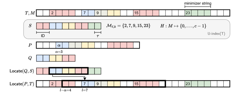
Figure 2: An illustration of the U-index of a text $T$, along with a query example. First, the minimizers $M$ of $T$ are found, here of length $k=4$ characters, with two of them overlapping (those starting at positions 7 and 9). The minimizer positions $\mathcal{M}_{\ell,k}$ are stored with Elias-Fano coding. Minimizers are hashed via $H$ to shorter IDs. These are padded to the next multiple of $\tau$. An index is then built on the sketch $S$. To locate a pattern $P$, its minimizers are found and the sketch $Q$ of corresponding IDs is constructed. Then $Q$ is located in $S$, which here gives a single match. The first minimizer of the match in $Q$ is located in $T$ at position $l$ via $\mathcal{M}_{\ell,k}$. Lastly, the candidate match is verified starting at position $l-\alpha$ in $T$.

Theoretical Guarantees. We now explain how to verify an occurrence at position $p\in L^{\prime}$ in $\mathcal{O}(1)$ time and using $\mathcal{O}(z)$ space. Let the occurrence be $S[p\mathinner{.\,.}q]$ where $q=p+|Q|-1$.

For faster querying in theory or for very long patterns in practice, we also store an array $F$ of fingerprints, where $F[i]=\phi(T[0\mathinner{.\,.}p_{i}])$ for all $p_{i}\in\mathcal{M}_{\ell,k}(T)$, and $\phi$ is the rolling hash function; see Section˜2. This array can be constructed in $\mathcal{O}(n)$ time and has size $\mathcal{O}(z)$. Let $\mathcal{X}=\{T[p_{i}\mathinner{.\,.}p_{i}+\ell)\mid p_{i}\in\mathcal{M}_{\ell,k}(T)\}$ and $\mathcal{X}^{R}=\{T[p_{i}-\ell+1\mathinner{.\,.}p_{i}]^{R}\mid p_{i}\in\mathcal{M}_{\ell,k}(T)\}$, where $s^{R}$ denotes the reverse of the string $s$. We construct the tries $\mathcal{T}=\textup{{Trie}}(\mathcal{X})$ and $\mathcal{T}^{R}=\textup{{Trie}}(\mathcal{X}^{R})$. We label the leaf nodes representing the string $s=T[p_{i}\mathinner{.\,.}p_{i}+\ell)$ and $s^{R}=(T[p_{i}-\ell+1\mathinner{.\,.}p_{i}])^{R}$ in both tries by the set $X_{s}=\{p_{i}\mid T[p_{i}\mathinner{.\,.}p_{i}+\ell)=s\wedge p_{i}\in\mathcal{M}_{\ell,k}\}$. Each leaf is also assigned a lex-rank that is obtained via an in-order DFS traversal of the trie. We also implement an inverse function that takes $p_{i}$ as input and returns the lex-rank of the leaf node that represents $s=T[p_{i}\mathinner{.\,.}p_{i}+\ell)$ in $\mathcal{T}$. We implement the analogous inverse function for $\mathcal{T}^{R}$. Each branching node $u$ in $\mathcal{T}$ stores an interval whose left and right endpoints are the lex-rank of the leftmost and rightmost leaf node, respectively, in the subtree rooted at $u$. This information is also computed via a DFS traversal. We store the analogous information for the branching nodes in $\mathcal{T}^{R}$. Since $\mathcal{T}$ and $\mathcal{T}^{R}$ are compacted and $\sum|X_{s}|=z$, it follows that the tries and the inverse functions take $\mathcal{O}(z)$ space. The tries and the inverse functions can be constructed in $\mathcal{O}(n)$ time [7].

Let us explain how these additional structures can help us verify an occurrence $S[p\mathinner{.\,.}q]$ of $Q$ in $S$ in $\mathcal{O}(1)$ time; see Figure˜3. Let $l:=\mathcal{M}_{\ell,k}(T)[p/b]$ and $r:=\mathcal{M}_{\ell,k}(T)[q/b]$. Using the vector $F$, we compute $\phi(T[l+1\mathinner{.\,.}r])$ in $\mathcal{O}(1)$ time for Fact 1, because we have $F[l]=\phi(T[0\mathinner{.\,.}l])$ and $F[r]=\phi(T[0\mathinner{.\,.}r])$. We also compute the fingerprint $\phi(P[\alpha+1\mathinner{.\,.}\beta])$ once in $\mathcal{O}(m)$ time and compare the two fingerprints in $\mathcal{O}(1)$ time. If they are not equal, then $(l-\alpha)$ is not a valid occurrence. If they are equal, we need to check $P[0\mathinner{.\,.}\alpha]$ and $P[\beta\mathinner{.\,.}m)$. The remaining letters on each edge cannot be more than $\ell$ (by the density of the minimizers mechanism), and so the verification would cost $\mathcal{O}(\ell)$ time if we did it by letter comparisons. We can verify the edges in $\mathcal{O}(1)$ time using tries. In a preprocessing step, we spell $P[\beta\mathinner{.\,.}m)$ in $\mathcal{T}$ arriving at node $u$; and we spell $(P[0\mathinner{.\,.}\alpha])^{R}$ in $\mathcal{T}^{R}$ arriving at node $u^{\prime}$. We can then check whether $r$ is a leaf node in the subtree induced in $\mathcal{T}$ using the inverse function and the interval stored in $u$. We can also check whether $l$ is a leaf node in the subtree induced in $\mathcal{T}^{R}$ using the inverse function and the interval stored in $u^{\prime}$. This takes $\mathcal{O}(1)$ time per pair $(l,r)$. We then have that $(l-\alpha)$ is a valid occurrence if and only if both leaf nodes are located in the induced subtrees.

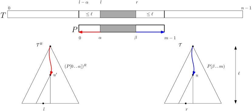
Figure 3: The $\mathcal{O}(1)$-time verification algorithm for occurrence $l-\alpha$. After spelling the fragments of $P$ in the two tries once, we check if the fragments in gray match using fingerprints in $\mathcal{O}(1)$ time; if so, we check if the corresponding leaf nodes are both located in the induced subtrees in $\mathcal{O}(1)$ time.

We have thus arrived at the following result.

Theorem 4.1.

(Universal framework) Let $T$ be a string of length $n$ over alphabet $\Sigma=[0,\sigma)$. Let $t(n,\sigma)$, $s(n,\sigma)$, and $q(m,n,\sigma)$ be, respectively, the time complexity to construct Index, the size of Index in machine words, and the query time of Index to report all the occurrences of a pattern of length $m$ in $T$. Furthermore, let $z:=|\mathcal{M}_{\ell,k}(T)|$ be the number of minimizers of $T$, for some parameters $\ell,k$, and let $S$ be the string obtained from $T$ using the framework with a parameter $\tau$ chosen from $[1,\log_{2}(n)]$. Then, in $\mathcal{O}(n+t(z\lceil\log z/\tau\rceil,2^{\tau}))$ time, we can construct an index of $\mathcal{O}(z+s(z\lceil\log z/\tau\rceil,2^{\tau}))$ size, supporting $\textup{{Locate}}(P,T)$ queries for a pattern $P$ of length $m\geq\ell$ in $\mathcal{O}(m+q(|Q|,z\lceil\log z/\tau\rceil,2^{\tau})+\textup{{Count}}(Q,S))$ time, where $Q$ is the string obtained from $P$ using the framework with parameters $\ell,k,\tau$.

Example. Let us now consider a practical instantiation of Theorem˜4.1. Let Index be the suffix array [28] enhanced with the longest common prefix (LCP) array [25]. We choose $\tau:=\lceil\log_{2}n\rceil$ because the suffix array can be constructed in $t(n,2^{\tau})=\mathcal{O}(n)$ time, for any integer alphabet of size $2^{\tau}\leq n$, and it has size $s(n,2^{\tau})=\mathcal{O}(n)$ [23]. Given the suffix array, the LCP array can be constructed in $\mathcal{O}(n)$ time [25]. By applying Theorem˜4.1, we construct a string $S$ of length $z\leq n$ over the alphabet $[0,n)$. Thus, we will construct our index in $\mathcal{O}(n+t(z,n))=\mathcal{O}(n)$ time of $\mathcal{O}(z+s(z,n))=\mathcal{O}(z)$ size. Note that, by using minimizers [31, 32], $z$ can be much smaller than $n$ in practice, for a sufficiently large value of $\ell$. Specifically, we have $z=nd$ where $d\geq 1/(\ell-k+1)$ is the density of the specific minimizer scheme used. For querying, we have $q(m,n,\sigma)=\mathcal{O}(m+\log n+\textup{{Count}}(P,T))$ when LCP information is used [28]. Thus, our query time is $\mathcal{O}(m+\log z+\textup{{Count}}(Q,S))$ because $m\geq|Q|$ and $\textup{{Count}}(Q,S)\geq\textup{{Count}}(P,T)$. Note that although $\textup{{Count}}(Q,S)\geq\textup{{Count}}(P,T)$, we also have $\log z\leq\log n$, and so beyond space savings, the resulting index can also be competitive or faster in querying.

5 Experiments

We implemented the U-index framework in the Rust programming language. In Section˜5.1, we present the setup of the experiments that we conducted to assess the efficiency of our implementation. In Section˜5.2, we present the results of these experiments. In Section˜5.3, we present an application of our framework in mapping long reads onto a reference genome.

Our software resources are open-source and can be found at https://github.com/u-index/u-index-rs.

Implementation Details. In practice, we verify each candidate occurrence using a linear scan of $P$ in $T$, hence without using any trie data structure. Even if this solution costs $\mathcal{O}(m)$ time instead of the $\mathcal{O}(1)$-time verification claimed by Theorem 4.1, this is likely to be faster in practice because traversing tries is not cache-efficient.

5.1 Setup

Hardware and Software. All experiments were run on an Intel Core i7-10750H running at a fixed frequency of 2.6 GHz with hyperthreading disabled and cache sizes of 32 KiB (L1), 256 KiB (L2), and 12 MiB (shared L3). Code was compiled using rustc 1.85.0-nightly and GCC 14.2.1 on Arch Linux.

Datasets. We use three textual datasets of different nature and alphabet size: (1) chromosome 1 of CHM13v2.0, which contains repetitive regions and consists of 248 million symbols over the DNA alphabet ($\sigma=4$), thus 59 MiB when each symbol is coded using 2 bits; (2) the 200 MiB protein sequences available from the Pizza & Chili site ($\sigma=27$), or 125 MiB when each symbol is coded using 5 bits; and (3) the 200 MiB English collection, also available from the Pizza & Chili site ($\sigma=239$). In the following, we discuss experimental results referring to Figure˜4 (at page 4) for the DNA alphabet. The results for proteins and English have very similar shapes and are deferred to Appendix˜B due to space constraints.

Queries. For each dataset, we test $10^{5}$ positive queries that are uniformly sampled from the text. For DNA, queries consist of $512$ characters, while for the protein and English datasets we use queries of $128$ characters.

Tested Indexes. We compare the suffix array and the FM-index, indicated with SA and FM-index in our results, against their U-index variants, with parameters $(k,\ell)\in\{(4,32),(8,64),(16,128),(28,256)\}$. For the suffix array construction, we use libsais [30, 22]. For the FM-index, we use the implementations in SDSL-lite (SDSL-v2) [15] and in AWRY [1].

For each index, we use the smallest $\tau\geq\lceil\log_{2}c\rceil$ that is supported by the index. In practice, this means that for the suffix array and SDSL FM-index we use $\lceil\log_{2}c/8\rceil$ bytes to represent each ID, so that each ID is a single character. This way, these indexes get built on exactly $z=|\mathcal{M}_{\ell,k}(T)|$ characters. In practice, this is strictly better than using a smaller $\tau$ and building an index on $2z$ or more characters. The AWRY FM-index does not support generic alphabets, and thus we had to consistently use $\tau=2$ to encode the IDs as DNA bases. We note that the AWRY uses a multi-threaded parallel construction algorithm, while all other methods are single-threaded. Further details can be found in Appendix˜A.

Finally, we also compare against our own implementation of the sparse suffix array at minimizer positions [16], that we call the sparse SA index in our results.

5.2 Results

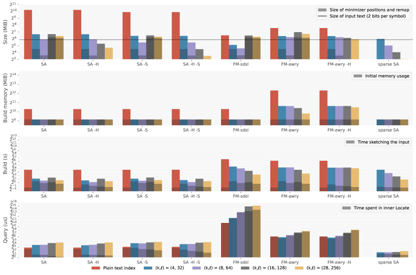
Figure 4: Results on the $59$ MiB of the human chromosome 1. For each data structure — except the sparse SA — we compare its performance when constructed on the plain input text (in red, left column of each group) versus when used with the U-index (remaining colors and columns), for increasing values of $k$ and $\ell$. Indexes marked with -H (read, “minus H”) use minimizers themselves as IDs, without the map $H$. Similarly, the indexes marked with -S omit storing the sketched input text $S$ and instead reconstruct it via the minimizer positions $\mathcal{M}_{\ell,k}(T)$ and $T$ itself. The sparse SA is only shown with sampling (no red column) because it is otherwise equivalent to SA. The top plot shows space usage of the final data structure in MiB, with the space for minimizer positions and the map $H$ shaded and the black line indicating the space occupied by the 2-bit packed input text. The second row shows the maximum memory usage (resident set size, RSS) during the construction, where the shaded area is memory usage before construction. The third row shows build time (in seconds), with the time for sketching the input shaded. The bottom plot shows query time (in average $\mu$s per Locate query), with the time for searching in the inner index shaded.

Suffix Array. In all cases, we see that the U-index variants take less space and are faster to construct than the classic indexes. Both space and construction time tend to be at least $8\times$ less. The time spent searching the suffix array (bottom, shaded) goes down as the suffix array becomes sparser, but the total query time goes up. This is due to the increasing number of false positive matches in minimizer space, starting at $10$ false positives per query for $(k,\ell)=(4,32)$ and going up to $100$ for $(k,\ell)=(28,256)$. These are caused by highly repetitive regions in the centromere [17]. Nevertheless, query time is usually less than twice slower than the classic suffix array, while space and construction time are greatly reduced.

Omitting $H$. When $k\in\{16,28\}$, most minimizers are unique, and the map $H$ mapping the minimizers to IDs has size linear in their number. This can be seen in that the shaded area in the rightmost two columns of the top-left group is accountable for most of the space used by the index at over $2^{6}=64$ MiB, while the input only takes 59 MiB when encoded using $2$ bits per character. Looking at SA -H, which omits $H$, we see that the index is much smaller for larger $k$, while query time is unaffected. Construction time does increase, since the alphabet is larger and hence requires more memory. The high spike for $k=16$ seems to be caused by SA (libsais) being particularly slow for 32-bit integers.

Implicit Sketched Text. We can also omit the sketched text $S$ and instead reconstruct it on-the-fly, as explained in Section˜4. This saves significant space when $k$ is large (where also $H$ can be omitted altogether). Construction time is not affected since $S$ is discarded after construction. The time spent in searching the suffix array does increase significantly though, up to $4\times$ (shaded), but as most of the time is spent verifying potential matches, the total query time only goes up slightly.

FM-index. The SDSL implementation takes around 90 MiB for the plain input text, and goes significantly below this when using the U-index. Construction time improves as well, almost $2\times$ each time we double $\ell$ because the number of sampled positions nearly halves.

A main drawback of the SDSL implementation is its significantly larger query times compared to all other methods, starting at $32\times$ slower for the plain index and increasing up to $1000\times$ slower for $\ell=256$. We suspect this is due to the inherent complexity in the wavelet tree data structures used to represent the Burrows-Wheeler transform of the text [6], that has increasingly more levels as $k$ increases and hence the number of bits $\tau$ in each $k$-mer ID grows. This makes SDSL an impractical choice in this scenario or, more in general, for applications where size is not a bottleneck but fast queries are the primary concern.

AWRY uses around twice as much space as SDSL, and has a similar construction time, likely because both are limited by the internal suffix array construction. On the other hand, query times for AWRY are significantly faster than SDSL because AWRY is optimized for the DNA alphabet, and the U-index version with $k=4$ is slightly faster than AWRY on the plain text. However, as $k$ and $\ell$ increase, both SDSL and AWRY slow down by roughly a factor of 2 overall. For AWRY we can also omit $H$ and this almost halves the size when $k$ is large, but negates the previously seen speedup in construction time since the sketched input $S$ is significantly larger.

Sparse SA. Lastly, the sparse SA index takes strictly less space than the U-index variant of the suffix array, since it stores strictly less information: only one permutation of the minimizer positions in the original text. It is also significantly faster to query, since no sketching is needed. Additionally, it has much fewer false positives, since comparisons are made in the plain input space rather than in sketch-space. Construction time is worse than SA however, since there is no known linear-time implementation for sparse suffix array construction. Nevertheless, this is still faster than constructing an FM-index.

5.3 An Example Application

To show a concrete application of our framework, we show that U-index can be used for long-read mapping. This is the problem of aligning long DNA or RNA sequencing reads (e.g., of length more than 1,000 base pairs) to a reference genome. Although long reads offer significant advantages over short reads in many crucial tasks in bioinformatics, such as genome assembly or structural variant detection, their alignment is computationally costly.

Setup. We run the following experiment. As input, we take the full human genome (CHM13v2.0) and a prefix of 450 PacBio HiFi long reads from the HG002-rep1 dataset. These reads are approximately 99.9% accurate and have an average length of 16kbp.

We partition (chunk) each read into patterns of length 256, and search each of these patterns in our index. Short leftover suffixes are ignored. Ideally, each read has then at least one pattern that exactly matches the text, which can then be used to anchor an alignment.

Results. We build the U-index on top of the libsais suffix array in the configuration where the minimizer space sequence $S$ and map $H$ are both stored. We use $k=8$ and $\ell=128$, so that at least 2 and on average 4 minimizers are sampled from every pattern. This results in 53M minimizers, and the entire U-index is built in 12 seconds.

Out of the 450 sequences, 445 have at least one matching pattern, and in total, 14 824 of the 28 243 patterns match (52%). As observed before, an issue with DNA is that it contains many long repetitive regions. In particular, 160 of the patterns each match around 3820 times for a total of 611k matches, while the 28k remaining patterns only match 27k in total. Worse, there are 721M mismatches, i.e., candidate matches in sketch-space that turn out not to be matches in the genome. Verifying these candidate matches takes over 98% of the time.

Limiting Matches. Only very few (<200) patterns have more than 10 matches, and thus we stop searching once we hit 10 matches. Further, most patterns have relatively few mismatches, while a few patterns have a lot of mismatches. To also avoid those negative effects, we generally only consider the first 100 matches in sketch-space. We still match 445 of 450 reads, while the number of matched patterns goes down to 13 717. On the other hand, the number of mismatches is now 663k (23 per query) and the number of matches is 25k (0.9 per query).

The result is a query time of 8.7$\mu$s per pattern or 550$\mu$s per read, of which 33% is sketching the input, 18% is locating the sketch, and the remaining 48% is verification.

6 Conclusions and Future Work

In this work, we introduced the U-index — a universal framework to enhance the performance of any off-the-shelf text index, provided that the patterns to match are sufficiently long. This is achieved, in short, by sketching the text and using any desired index for the sketched text. Intuitively, this saves resources at building time and considerably reduces the final index size, simply because the sketched text is shorter than the input text. Our experiments indeed confirm that the U-index has excellent performance when used in combination with the suffix array, as it significantly improves index size and construction while not slowing down queries too much. When paired with the FM-index, the savings are more modest but still significant.

The sparse suffix array index by Grabowski and Raniszewski [16] remains a great solution in this regime, having smaller size and significantly faster queries than the U-index around suffix arrays (which have, however, faster construction time). For example, albeit somewhat larger than the SDSL FM-index, the sparse suffix array is over $100\times$ faster to query. However, the benefit of the U-index framework lies in its universality and usability. We remark that the primary objective of this work is to highlight these two important properties.

We anticipate that the U-index may be especially useful around the r-index [14] when used on highly repetitive data, but we leave this as future work. The sparse suffix array will by design be unable to take advantage of the underlying repetitiveness. Hence, other than universality, another important virtue of our framework is that it preserves string similarity: for any two highly similar texts $T_{1}$ and $T_{2}$, it will be the case that $S_{1}=\textup{{Sketch}}(T_{1})$ and $S_{2}=\textup{{Sketch}}(T_{2})$ are also highly similar (assuming the sketches are based on minimizers).

In terms of theory, it would make sense to bound $\textup{{Count}}(Q,S)$ as a function of $\textup{{Count}}(P,T)$ and the sketching parameters. Such a function would bound the number of false positives.

Appendix A Further Details on Tested Indexes and the $\tau$ Values

Here we explain in more detail how each of the indexes was used.

The libsais Suffix Array. For the plain input, including for DNA, we use a $\tau=8$ byte encoding. For the sketched text $S$, this depends on $c$. When $\log_{2}(c)\leq 8$, we use one-byte encoding and call the libsais function. When $\log_{2}(c)\leq 16$, we use two-byte encoding and call libsais16. For larger $c$, we first remap all IDs to values starting at $0$, as recommended by the library authors, and then call the function libsais_int on 32-bit input values.

The SDSL-lite FM-index. For the plain text, we use the Huffman-shaped wavelet tree with default parameters, i.e., the class csa_wt<wt_huff<rrr_vector<63>>,32,64>. For the U-index counterpart, we instead use csa_wt<wt_int<rrr_vector<63>>,32,64>, a wavelet-tree over a variable-width integer alphabet. Both these indexes use a sampling factor of $32$ to sample the suffix array. Also, for both versions we remap $k$-mers to ids starting at $1$ instead of $0$, since SDSL does not support input values of $0$. For this reason, we do not have a -H no-remap variant of the SDSL FM-index.

The AWRY FM-index. The AWRY FM-index only supports DNA and protein alphabets. For consistency, we only use the DNA version. This means that we consistently use $\tau=2$. Thus, IDs with $\log_{2}(c)$ bits are encoded into $\lceil\log_{2}(c)\rceil$ DNA bases, which are passed to AWRY as 8-bit ACGT characters. Similarly, plain text protein and English input is encoded into 4 underlying characters. This index also uses a suffix array sampling factor of $32$.

The sparse SA. The sparse SA consists of an array of 32-bit integers indicating text positions. It is constructed using the Rust standard library Vec<u32>::sort_unstable_by_key function that compares text indices by comparing the corresponding suffixes.

Appendix B Experimental Results on Proteins and English Datasets

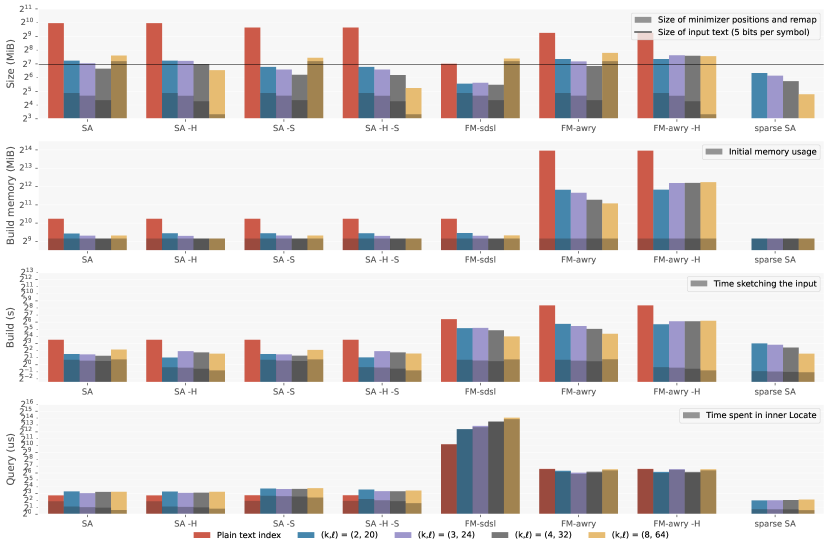
Figure 5: Results on $200$ MiB of protein sequences. Refer to the caption of Figure˜4.

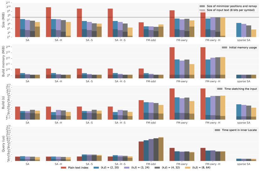
Figure 6: Results on $200$ MiB of English text. Refer to the caption of Figure˜4.

References

- [1] Tim Anderson and Travis J Wheeler. An optimized FM-index library for nucleotide and amino acid search. Algorithms for Molecular Biology, 16(1):25, 2021.
- [2] Lorraine A. K. Ayad, Grigorios Loukides, and Solon P. Pissis. Text indexing for long patterns: Anchors are all you need. Proc. VLDB Endow., 16(9):2117–2131, 2023.
- [3] Lorraine A. K. Ayad, Grigorios Loukides, and Solon P. Pissis. Text indexing for long patterns using locally consistent anchors. CoRR, abs/2407.11819, 2024.
- [4] Lorraine A. K. Ayad, Grigorios Loukides, Solon P. Pissis, and Hilde Verbeek. Sparse suffix and LCP array: Simple, direct, small, and fast. In José A. Soto and Andreas Wiese, editors, LATIN 2024: Theoretical Informatics - 16th Latin American Symposium, Puerto Varas, Chile, March 18-22, 2024, Proceedings, Part I, volume 14578 of Lecture Notes in Computer Science, pages 162–177. Springer, 2024.
- [5] Christina Boucher, Travis Gagie, Alan Kuhnle, Ben Langmead, Giovanni Manzini, and Taher Mun. Prefix-free parsing for building big BWTs. Algorithms for Molecular Biology, 14(1), May 2019.
- [6] Michael Burrows and David Wheeler. A block-sorting lossless data compression algorithm. In Digital SRC Research Report. Citeseer, 1994.
- [7] Panagiotis Charalampopoulos, Costas S. Iliopoulos, Chang Liu, and Solon P. Pissis. Property suffix array with applications in indexing weighted sequences. ACM J. Exp. Algorithmics, 25:1–16, 2020.
- [8] Francisco Claude, Gonzalo Navarro, Hannu Peltola, Leena Salmela, and Jorma Tarhio. String matching with alphabet sampling. J. Discrete Algorithms, 11:37–50, 2012.
- [9] Martin Dietzfelbinger, Joseph Gil, Yossi Matias, and Nicholas Pippenger. Polynomial hash functions are reliable (extended abstract). In Werner Kuich, editor, Automata, Languages and Programming, 19th International Colloquium, ICALP92, Vienna, Austria, July 13-17, 1992, Proceedings, volume 623 of Lecture Notes in Computer Science, pages 235–246. Springer, 1992.
- [10] Robert Edgar. Syncmers are more sensitive than minimizers for selecting conserved k-mers in biological sequences. PeerJ, 9(e10805):1755–1771, 2021.
- [11] Peter Elias. Efficient storage and retrieval by content and address of static files. Journal of the ACM, 21(2):246–260, 1974.
- [12] Robert Mario Fano. On the number of bits required to implement an associative memory. Memorandum 61, Computer Structures Group, MIT, 1971.
- [13] Paolo Ferragina and Giovanni Manzini. Indexing compressed text. J. ACM, 52(4):552–581, jul 2005.
- [14] Travis Gagie, Gonzalo Navarro, and Nicola Prezza. Fully functional suffix trees and optimal text searching in bwt-runs bounded space. J. ACM, 67(1), jan 2020.
- [15] Simon Gog, Timo Beller, Alistair Moffat, and Matthias Petri. From theory to practice: Plug and play with succinct data structures. In Experimental Algorithms: 13th International Symposium, SEA 2014, Copenhagen, Denmark, June 29–July 1, 2014. Proceedings 13, pages 326–337. Springer, 2014.
- [16] Szymon Grabowski and Marcin Raniszewski. Sampled suffix array with minimizers. Softw. Pract. Exp., 47(11):1755–1771, 2017.
- [17] Deborah L Grady, Robert L Ratliff, Donna L Robinson, Erin C McCanlies, Julianne Meyne, and Robert K Moyzis. Highly conserved repetitive dna sequences are present at human centromeres. Proceedings of the National Academy of Sciences, 89(5):1695–1699, 1992.
- [18] Ragnar Groot Koerkamp and Giulio Ermanno Pibiri. The mod-minimizer: A Simple and Efficient Sampling Algorithm for Long k-mers. In Solon P. Pissis and Wing-Kin Sung, editors, 24th International Workshop on Algorithms in Bioinformatics (WABI 2024), volume 312 of Leibniz International Proceedings in Informatics (LIPIcs), pages 11:1–11:23, Dagstuhl, Germany, 2024. Schloss Dagstuhl – Leibniz-Zentrum für Informatik.
- [19] Roberto Grossi and Jeffrey Scott Vitter. Compressed suffix arrays and suffix trees with applications to text indexing and string matching. SIAM Journal on Computing, 35(2):378–407, 2005.
- [20] Dan Gusfield. Algorithms on stings, trees, and sequences: Computer science and computational biology. Acm Sigact News, 28(4):41–60, 1997.
- [21] Aaron Hong, Marco Oliva, Dominik Köppl, Hideo Bannai, Christina Boucher, and Travis Gagie. Acceleration of FM-Index Queries Through Prefix-Free Parsing. Schloss Dagstuhl – Leibniz-Zentrum für Informatik, 2023.
- [22] Juha Kärkkäinen, Giovanni Manzini, and Simon J Puglisi. Permuted longest-common-prefix array. In Combinatorial Pattern Matching: 20th Annual Symposium, CPM 2009 Lille, France, June 22-24, 2009 Proceedings 20, pages 181–192. Springer, 2009.
- [23] Juha Kärkkäinen, Peter Sanders, and Stefan Burkhardt. Linear work suffix array construction. J. ACM, 53(6):918–936, 2006.
- [24] Richard M. Karp and Michael O. Rabin. Efficient randomized pattern-matching algorithms. IBM J. Res. Dev., 31(2):249–260, 1987.
- [25] Toru Kasai, Gunho Lee, Hiroki Arimura, Setsuo Arikawa, and Kunsoo Park. Linear-time longest-common-prefix computation in suffix arrays and its applications. In Amihood Amir and Gad M. Landau, editors, Combinatorial Pattern Matching, 12th Annual Symposium, CPM 2001 Jerusalem, Israel, July 1-4, 2001 Proceedings, volume 2089 of Lecture Notes in Computer Science, pages 181–192. Springer, 2001.
- [26] Grigorios Loukides and Solon P. Pissis. Bidirectional string anchors: A new string sampling mechanism. In Petra Mutzel, Rasmus Pagh, and Grzegorz Herman, editors, 29th Annual European Symposium on Algorithms, ESA 2021, September 6-8, 2021, Lisbon, Portugal (Virtual Conference), volume 204 of LIPIcs, pages 64:1–64:21. Schloss Dagstuhl - Leibniz-Zentrum für Informatik, 2021.
- [27] Grigorios Loukides, Solon P. Pissis, and Michelle Sweering. Bidirectional string anchors for improved text indexing and top- similarity search. IEEE Trans. Knowl. Data Eng., 35(11):11093–11111, 2023.
- [28] Udi Manber and Eugene W. Myers. Suffix arrays: A new method for on-line string searches. SIAM J. Comput., 22(5):935–948, 1993.
- [29] Gonzalo Navarro and Veli Mäkinen. Compressed full-text indexes. ACM Computing Surveys (CSUR), 39(1):2–es, 2007.
- [30] Ge Nong, Sen Zhang, and Wai Hong Chan. Two efficient algorithms for linear time suffix array construction. IEEE transactions on computers, 60(10):1471–1484, 2010.
- [31] Michael Roberts, Wayne Hayes, Brian R. Hunt, Stephen M. Mount, and James A. Yorke. Reducing storage requirements for biological sequence comparison. Bioinform., 20(18):3363–3369, 2004.
- [32] Saul Schleimer, Daniel Shawcross Wilkerson, and Alexander Aiken. Winnowing: Local algorithms for document fingerprinting. In Alon Y. Halevy, Zachary G. Ives, and AnHai Doan, editors, Proceedings of the 2003 ACM SIGMOD International Conference on Management of Data, San Diego, California, USA, June 9-12, 2003, pages 76–85. ACM, 2003.
- [33] Hongyu Zheng, Carl Kingsford, and Guillaume Marçais. Improved design and analysis of practical minimizers. Bioinformatics, 36(Supplement_1):i119–i127, 2020.