Polycyclic Geometric Realizations of the Gray Configuration

Abstract

The Gray configuration is a $(27_{3})$ configuration which typically is realized as the points and lines of the $3\times 3\times 3$ integer lattice. It occurs as a member of an infinite family of configurations defined by Bouwer in 1972. Since their discovery, both the Gray configuration and its Levi graph (i.e., its point-line incidence graph) have been the subject of intensive study. Its automorphism group contains cyclic subgroups isomorphic to $\mathbb{Z}_{3}$ and $\mathbb{Z}_{9}$, so it is natural to ask whether the Gray configuration can be realized in the plane with any of the corresponding rotational symmetry. In this paper, we show that there are two distinct polycyclic realizations with $\mathbb{Z}_{3}$ symmetry. In contrast, the only geometric polycyclic realization with straight lines and $\mathbb{Z}_{9}$ symmetry is only a “weak” realization, with extra unwanted incidences (in particular, the realization is actually a $(27_{4})$ configuration).

Keywords: Gray graph, Gray grid, Levi graph, reduced Levi graph, semi-regular subgroup, Pappus graph, pseudoline realization.

Math. Subj. Class. (2020): 05B30, 05C10, 05C60, 51A45, 51E30.

1 Introduction

The Gray graph was discovered by Marion C. Gray in 1932, and was rediscovered independently by Bouwer when searching for regular graphs that are edge-transitive but not vertex-transitive [6]; graphs fulfilling these conditions are called semisymmetric [23]), so henceforth we use this term. A first detailed study of semisymmetric graphs is due to Folkman [12]. The Gray graph, in particular, also became the subject of a careful investigation: the third author of this paper and his co-workers explored many interesting properties of this graph [20, 21, 23, 24]; see also [26, Chapter 6] (for more details about its history, see [23]). We know that it is the smallest trivalent semisymmetric graph. Its girth is 8, which is equivalent to saying that the Gray configuration is triangle-free. It is Hamiltonian, with a Hamiltonian realization displaying a $\mathbb{Z}_{9}$ symmetry, as a construction due to Randić reveals it [20, 25]. A corresponding LCF notation is $[7,-7,13,-13,25,-25]^{9}$. This can be clearly seen in Figure 1.

Figure 1: The Gray graph. The square nodes correspond to lines and the circular nodes correspond to points; the coloring demonstrates rotational $\mathbb{Z}_{9}$ symmetry. This is further explored in Section 7.

The Gray configuration is a $(27_{3})$ configuration which occurs as a member of an infinite family of configurations defined by Bouwer in 1972 [6, Section 1]. Its name stems from the fact that its Levi graph—that is, the point-line incidence graph—is the Gray graph; see Figure 1. (While it may appear that the graph has dihedral symmetry, this is not the case, because the mirror symmetry interchanges line-nodes and point-nodes, and while the individual color classes have mirror symmetry, the graph as a whole does not.) By the definition due to Bouwer, it can be realized as a spatial configuration consisting of the 27 points and 27 lines of the $3\times 3\times 3$ integer grid (cf. Figure 2). It can also be conceived as the Cartesian product of three copies of the “dual pencil” $(3_{1},1_{3})$ configuration, or equivalently, the Cartesian product of the dual pencil $(3_{1},1_{3})$ and the $(9_{2},6_{3})$ “grid configuration” [13]. Together with its dual, it forms a pair of the smallest configurations which are triangle-free and flag transitive but not self-dual [21]. Moreover, it is resolvable. By definition, this means that the set of configuration lines partitions into classes (called resolution classes or parallel classes) such that within each class, the lines partition the set of points of the configuration by incidences [14]. This is clearly seen in Figure 2, since the parallel classes of the lines coincide with the parallel classes in geometric sense. The grid structure makes possible assigning labels to the configuration points of the form $xyz$ $(x,y,z\in\mathbb{Z}_{3})$ such that two points with labels $xyz$ and $x^{\prime}y^{\prime}z^{\prime}$ are incident to the same line if and only if precisely two of the equalities $x=x^{\prime}$, $y=y^{\prime}$, $z=z^{\prime}$ hold.

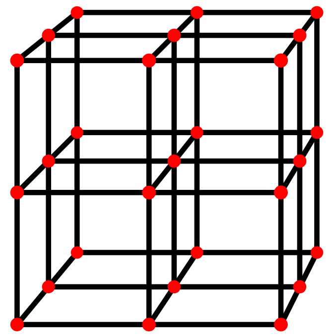
Figure 2: Spatial realization of the Gray configuration.

A polycyclic geometric realization of a configuration of points and lines is one in which (1) the combinatorial lines of the configuration are represented in the Euclidean plane using straight lines; (2) the points and lines are divided into symmetry classes in which each symmetry class contains the same number of elements. That is, it is a realization of the configuration in which a semi-regular subgroup of the automorphism group maps the realization to itself.

The main results of this paper are

• to show that the Gray configuration can be realized polycyclically in two different ways with $\mathbb{Z}_{3}$ symmetry, realized as geometric rotation;

• to show that the Gray configuration can only be weakly polycyclically geometrically realized with $\mathbb{Z}_{9}$ symmetry (any straight-line realization forces extra incidences), but it can be topologically realized as a polycyclic realization using pseudolines;

• There are no other geometric polycyclic realizations of the Gray configuration.

2 The automorphism group of the Gray configuration

The automorphism group $\mathrm{Aut}\,G$ of the Gray graph is a group of order $1296=6^{4}$, which can be given in the following form:

$$(S_{3}\times S_{3}\times S_{3})\rtimes S_{3}\cong S_{3}\wr S_{3},$$ (1)

where $S_{3}$ is the symmetric group of degree 3. This has been established in the literature in a more general setting, see e.g. [24]. The automorphism group of the Gray configuration is the same, since the Gray configuration is not self-dual (so there are no color-exchanging automorphisms). Here we give an independent proof, focusing directly on simple geometric properties of the spatial realization of the configuration.

In this spatial realization, the configuration contains three pencils of parallel layers. Each of these layers forms a $(9_{2},6_{3})$ “grid” configuration. Within each parallel pencil there are three layers, and these pencils are perpendicular (say) to the $x$-, $y$-, respectively the $z$-axis of a Cartesian coordinate system (note that the labels introduced in the previous section can be conceived as coordinates with respect to such a coordinate system in the Euclidean 3-space). Each of the three copies of the $S_{3}$ group in the parenthesis of (1) is responsible for permuting the layers within a given pencil (independently of each other, which explains why direct products are used). Note that this product in the parenthesis does not move one pencil to any other pencil. On the other hand, the second term of the semidirect product is responsible for permuting the three pencils, each as a whole (while leaving fixed the order of the layers within a pencil). In addition, it is easily seen that the group on the left (i.e. the triple direct product in the parenthesis) is an invariant subgroup of the entire group (while this does not hold for the right term). This explains why we use here semidirect product. Finally, it is well known that the semidirect product of the form above can be rewritten in the form of a wreath product of two copies of $S_{3}$.

3 Finding possible quotient graphs and reduced Levi graphs from semi-regular subgroups

Although we are interested mainly in polycyclic configurations, we first briefly consider the general case of semi-regular groups.

The automorphism group $\mathrm{Aut}\,G$ of a simple graph $G$ may be viewed as a group of permutations acting on the set of vertices of $G$. Its orbits induce a partition of the set of vertices of $G$. The action of a nontrivial subgroup $\Gamma\subseteq\mathrm{Aut}\,G$ is semi-regular if all of its orbits have the same cardinality $|\Gamma|$. Note that this is equivalent to saying that the stabiliser of $\Gamma$ is trivial; see [10]. For more information on this and what follows, see [10, 26].

A subgroup of $\text{Aut}\,G$ with a semi-regular action on the vertices of $G$ is called a semi-regular subgroup. All nontrivial subgroups of a semi-regular group are semi-regular. In particular, each nontrivial element $\alpha$ of a semi-regular group is a generator of a semi-regular cyclic group. Hence $\alpha$ is a semi-regular permutation. This is equivalent to saying that when writing a permutation $\alpha$ as a product of disjoint cycles, the length of all cycles is the same.

For any simple graph $G$ the action of $\Gamma\subseteq\mathrm{Aut}\,G$ on the vertex set extends to the actions on the set of edges (that is, undirected pairs of adjacent vertices) and the set of arcs or darts (that is, directed pairs of adjacent vertices). The action of a semi-regular subgroup can be described via quotient graphs. If $\Gamma$ is a semi-regular subgroup, then the graph $G/\Gamma$ is the quotient graph, with vertices in $G/\Gamma$ corresponding to orbits of vertices of $G$ under the action of $\Gamma$, and edges (including parallel edges, semi-edges, loops) determined by orbits of arcs of $G$, in the standard way, and the projection $\pi:G\rightarrow G/\Gamma$ is called a regular covering projection (see [16, 26, 10]). In the special case of a cyclic group $\Gamma$, we may consider its generator permutation $\alpha$. If $\alpha$ is a semi-regular automorphism, then the graph $G/\alpha$ is the quotient graph, with vertices in $G/\alpha$ corresponding to orbits of vertices of $G$ under the action of $\alpha$, etc.

Definition 1.

A simple graph $G$ of order $n$ admitting a semi-regular automorphism $\alpha$ of order $m$ is polycirculant. If $m=n$, the automorphism $\alpha$ is regular.

Remark 1.

Note that in the Definition above, $m$ divides $n$, and the quotient graph $G/\alpha$ has order $k$, where $n=mk$.

The renowned theorem of Sabidussi [27] states that a graph $G$ is a Cayley graph if and only if $\mathrm{Aut}\,G$ admits a subgroup with regular action, which corresponds to the quotient graph $G/\Gamma$ having only a single vertex.

Remark 2.

Note that a semi-regular automorphism of a simple graph acts semi-regularly on vertices and arcs of a graph but not necessarily on the edges of a graph. The easiest way to check whether the action on the edges is semi-regular is via quotient graphs; the action is semi-regular on the edges if and only if the quotient graph has no semi-edges.

Given a graph $G$, it is possible to determine all distinct regular covering projections $\pi:G\rightarrow G/\Gamma$. The recipe is as follows.

First we generate all semi-regular group actions up to conjugacy. This can be easily done by SageMath/python/GAP, which has all ingredients readily available.

def generate_semi_regular_actions(G): ”””Given graph G, generate all semi-regular group actions.””” AutG = G.automorphism_group() for Gamma in AutG.conjugacy_classes_subgroups(): if Gamma.is_semi_regular(): yield Gamma

Using Sage [28] and the above algorithm, we determined that the Gray graph has 5 conjugacy classes of subgroups which produce bipartite quotient graphs; the groups are listed in Table 1 and the corresponding quotient graphs in Figure 3. Note that the Gray graph is unusual in the sense that all quotients arising from semi-regular actions are bipartite!

Table 1: Semi-regular subgroups of $\mathrm{Aut}\,G$ for the Gray graph.

ID	order	subgroup isomorphic to…	bipartite?
1	3	$\mathbb{Z}_{3}$	YES
2	3	$\mathbb{Z}_{3}$	YES
3	9	$\mathbb{Z}_{3}\times\mathbb{Z}_{3}$	YES
4	9	$\mathbb{Z}_{9}$	YES
5	27	$\mathbb{Z}_{9}\times\mathbb{Z}_{3}$	YES

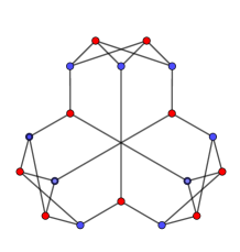
(a) Quotient with respect to $\mathbb{Z}_{3}$; the graph $GG$ (ID#1)

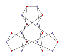
(b) Quotient with respect to $\mathbb{Z}_{3}$; the Pappus graph (ID#2)

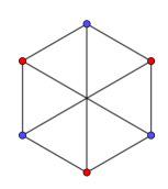
(c) Quotient with respect to $\mathbb{Z}_{3}\times\mathbb{Z}_{3}$ (ID#3)

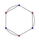
(d) Quotient with respect to $\mathbb{Z}_{9}$ (ID#4)

(e) Quotient with respect to $\mathbb{Z}_{9}\rtimes\mathbb{Z}_{3}$. (ID#5)

Figure 3: The five semi-regular quotient graphs of the Gray graph, and their IDs from Table 1. Since all quotients are bipartite, these graphs are all the possible RLGs of the Gray configuration.

Given a configuration, the incidence graph of the configuration, usually called a Levi graph, is formed by assigning one vertex of the graph to each point and line of the configuration, and joining vertices with edges if and only if the corresponding point and line are incident.

Definition 2.

A geometric realization of a configuration is polycyclic if there exists a semi-regular color-preserving automorphism $\alpha$ of the Levi graph $G$ that is realized by geometric rotation of the same order.

A reduced Levi graph (RLG) is a bipartite quotient of the Levi graph with a semi-regular subgroup of the automorphism group. We use the convention that arcs in reduced Levi graphs are directed from line-orbits to point-orbits. If you reverse all arrows in a reduced Levi graph and switch the interpretation of colors of nodes, the result is the reduced Levi graph of the dual configuration.

In the remainder of the paper, we determine which of the quotients of the Gray graph can be the reduced Levi graphs of polycyclic realizations of the Gray configuration, and we determine whether such geometric realizations exist.

4 Labeling elements of the Gray configuration and identifying the reduced Levi graphs

In what follows, we use the following labeling conventions. We label the points of the $3\times 3$ integer grid using the labels $ijk$, $i,j,k=0,1,2$ corresponding to the axes in $\mathbb{R}^{3}$, with the first, second, third coordinates corresponding to left-right, down-up, and front-back respectively.

The lines of the configuration are labeled $*ij=\{0ij,1ij,2ij\}$, $i\!*\!j=\{i0j,i1j,i2j\}$, and $ij*=\{ij0,ij1,ij2\}$. See Figure 4.

Figure 4: The Gray Grid: the points and lines of the Gray configuration, viewed as points and lines on the $3\times 3$ integer grid.

The labels, separated into symmetry classes, are shown in Table 2. Note that going from $R_{ij}$ to $R_{(i+1)j}$ ($B,G$ respectively) corresponds to adding 111, and going from $R_{ij}$ to $R_{i(j+1)}$ corresponds to adding 210 (with index arithmetic and point arithmetic all happening mod 3).

For the lines, adding an index also corresponds to adding 111 or 210 respectively, but ignoring the * component (that is, $*+i=*$ for $i=0,1,2$). For example, $X_{11}+210=*21+210=(*+2)(2+1)(1+0)=*01=X_{12}$ and $Y_{10}+111=2*1+111=(2+1)(*+1)(1+1)=0*2=Y_{20}$.

Table 2: The elements of the Gray configuration, labeled according to symmetry class over $\mathbb{Z}_{3}\times\mathbb{Z}_{3}$

$${\color[rgb]{1,0,0}\begin{array}[]{c c c}R_{00}=000&R_{01}=210&R_{02}=120\\ R_{10}=111&R_{11}=021&R_{12}=201\\ R_{20}=222&R_{21}=102&R_{22}=012\end{array}} \quad\begin{array}[]{c c c}X_{00}=*00&X_{01}=*10&X_{02}=*20\\ X_{10}=*11&X_{11}=*21&X_{12}=*01\\ X_{20}=*22&X_{21}=*02&X_{22}=*12\end{array}$$

$${\color[rgb]{0,0,1}\begin{array}[]{c c c}B_{00}=100&B_{01}=010&B_{02}=220\\ B_{10}=211&B_{11}=121&B_{12}=001\\ B_{20}=022&B_{21}=202&B_{22}=112\end{array}} \quad{\color[rgb]{1,.5,0}\begin{array}[]{c c c}Y_{00}=1\!*\!0&Y_{01}=0\!*\!0&Y_{02}=2\!*\!0\\ Y_{10}=2\!*\!1&Y_{11}=1\!*\!1&Y_{12}=0\!*\!1\\ Y_{20}=0\!*\!2&Y_{21}=2\!*\!2&Y_{22}=1\!*\!2\end{array}}$$

$${\color[rgb]{0,0.6,0}\begin{array}[]{c c c}G_{00}=110&G_{01}=020&G_{02}=200\\ G_{10}=221&G_{11}=101&G_{12}=011\\ G_{20}=002&G_{21}=212&G_{22}=122\end{array}} \quad{\color[rgb]{0,1,1}\begin{array}[]{c c c}Z_{00}=11*&Z_{01}=02*&Z_{02}=20*\\ Z_{10}=22*&Z_{11}=10*&Z_{12}=01*\\ Z_{20}=00*&Z_{21}=21*&Z_{22}=12*\end{array}}$$

Figure 5: The Gray Grid labeled with the symmetry classes from Table 2.

Figure 5 shows the Gray Grid using the labels from Table 2. This choice of labeling corresponds to the reduced Levi graph over $\mathbb{Z}_{3}\times\mathbb{Z}_{3}$ shown in Figure 6 (see also Figure 3(c)), where the first copy of $\mathbb{Z}_{3}$ corresponds to increasing the row index in Table 2 (that is, to adding $+111$) and the second copy of $\mathbb{Z}_{3}$ corresponds to increasing the column index (that is, to adding $+210$).

In Figure 6, the reduced Levi graph is oriented so that all arrows go from line classes to point classes, as mentioned above. Voltages are indicated as ordered pairs $(a,b)\in\mathbb{Z}_{3}\times\mathbb{Z}_{3}$, where $L\xrightarrow{(a,b)}P$ corresponds to an edge between $L_{ij}$ and $P_{(i+a)(j+b)}$ in the unreduced Levi graph, for $P\in\{R,G,B\}$, $L\in\{X,Y,Z\}$, $i,j\in\{0,1,2\}$. Unlabeled edges have voltage $(0,0)$. Incrementing the first coordinate corresponds to increasing the row index (that is, to adding $+111$) and incrementing the second coordinate corresponds to increasing the column index (that is, to adding $+210$).

Figure 6: The reduced Levi graph for the Gray configuration with voltage group $\mathbb{Z}_{3}\times\mathbb{Z}_{3}$.

Expanding the second copy of $\mathbb{Z}_{3}$ (that is, having symmetry classes $\Box_{a0}$, $\Box_{a1}$, $\Box_{a2}$, $a\in\mathbb{Z}_{3}$, $\Box\in\{X,Y,Z,R,G,B\}$) gives a quotient whose underlying graph is isomorphic to the Pappus graph (see Figure 3(b)).

$\cong$

Figure 7: Expanding the second copy of $\mathbb{Z}_{3}$ (that is, having symmetry classes $\Box_{a0}$, $\Box_{a1}$, $\Box_{a2}$, $a\in\mathbb{Z}_{3}$, $\Box\in\{X,Y,Z,R,G,B\}$) gives a quotient whose underlying graph is isomorphic to the Pappus graph. Two realizations are shown, one where the expansion is obvious and one where the underlying graph uses a more standard realization of the Pappus graph.

Expanding the first copy of $\mathbb{Z}_{3}$ (that is, having symmetry classes $\Box_{0j}$, $\Box_{1j}$, $\Box_{2j}$, $j\in\mathbb{Z}_{3}$, $\Box\in\{X,Y,Z,R,G,B\}$) gives a quotient isomorphic to the graph $GG$ shown in Figure 3(a).

Figure 8: Expanding the first copy of $\mathbb{Z}_{3}$ (that is, having symmetry classes $\Box_{0j}$, $\Box_{1j}$, $\Box_{2j}$, $j\in\mathbb{Z}_{3}$) gives a quotient isomorphic to the graph $GG$. Again, two drawings are shown, one corresponding directly to the expansion and one obviously isomorphic to the drawing of $GG$ shown in Figure 3(a).

5 A polycyclic realization of the Gray Configuration with the Pappus RLG

In this section, we show that the $\mathbb{Z}_{3}$ quotient graph, which as an unlabeled graph, is isomorphic to the Pappus graph (Figure 3(b)), produces a polycyclic realization of the Gray graph with $\mathbb{Z}_{3}$ symmetry. Consider the re-drawing of the Pappus voltage graph shown in Figure 9, in which a particular Hamiltonian cycle is chosen to be on the boundary of the graph.

Figure 9: (Left) A drawing of the Pappus RLG using a Hamiltonian cycle on the boundary, used in producing a polycyclic realization of the Gray configuration whose reduced Levi graph is the Pappus RLG. (Right) Relabeling to zero out the boundary edges. In the construction of a corresponding polycyclic realization, yellow highlights correspond to incidences with one degree of freedom, green highlights to incidences that are determined, and the blue highlights to a final incidence that results from a continuity argument.

Two useful facts about voltage graphs (which reduced Levi graphs are), are the following: (1) Adding an element of the voltage group to all edges incident with a node in the voltage graph results in an isomorphic lift graph (roughly, it corresponds to changing the designation of the “0-th” element of a particular symmetry class), and (2) consequently, given any spanning tree in a voltage graph, it is possible to zero-out the labels on that spanning tree. See [26] for more detailed information, and [3], especially Figure 6, for a worked out example. Beginning with the Pappus graph drawn with a Hamiltonian cycle on the boundary shown in Figure 9, we add and subtract voltages as necessary around the perimeter to zero-out all but one of the voltages on the outside Hamiltonian cycle, which will make construction of the corresponding realization of the Gray configuration more tractable. (Specifically, we started, somewhat arbitrarily at the node $Z_{j2}$ and added +1 to each of the labels on the incident edges, which turned $Z_{j2}\xrightarrow{-1}B_{j1}$ into $Z_{j2}\to B_{j1}$ while also turning $Z_{j2}\xrightarrow{1}R_{j2}$ to $Z_{j2}\xrightarrow{2}R_{j2}$ and $Z_{j2}\to G_{j2}$ to $Z_{j2}\xrightarrow{1}G_{j2}$. Next, we added $-1$ to all the edges incident with $G_{j2}$, which zeroes out the previously assigned $Z_{j2}\xrightarrow{1}G_{j2}$ while modifying the other two edges, including the one which becomes $G_{j2}\xrightarrow{-1}X_{j0}$, which is zeroed out by adding +1 to $X_{j0}$, and so on around the boundary, until all but one of the edges in the boundary cycle has label 0.)

To construct a configuration with $\mathbb{Z}_{3}$ symmetry with this reduced Levi graph, we follow the same sort of construction techniques that were outlined in [3], beginning at point symmetry class $B_{j2}$ and proceeding counterclockwise around the boundary of the RLG. At each step except the last, we are doing one of the following:

• Initialization: construct the point class $B_{j2}$ as the vertices of a regular 3-gon centered at $\mathcal{O}$: specifically, let $B_{j2}=(\cos(2\pi j/3),\sin(2\pi j/3))$.

• Draw a line (class) arbitrarily through a point (class) (one degree of freedom, denoted by a yellow highlight on the corresponding edge);

• Place a point (class) arbitrarily on a previously drawn line class (one degree of freedom, denoted by a yellow highlight on the corresponding edge);

• Construct a line (class) as the join of two points (green highlight on the corresponding graph edges)

• Construct a point (class) as the meet of two lines (green highlight on the corresponding graph edges)

Each of these steps depends on at most two previously-constructed elements.

In the final step, according to the constructions in the RLG, we need to have the line $Z_{j0}$ be incident with point $G_{j0}$, $R_{j0}$ and $B_{(j-1)2}$ (cyan highlight on the corresponding graph edges, which we accomplish via a continuity argument.

The specific construction steps are as follows:

1. Construct $B_{j2}=(\cos(2\pi j/3),\sin(2\pi j/3))$.

2. Construct line $Y_{02}$ arbitrarily through $B_{02}$, and construct $Y_{j2}$ by rotating $Y_{02}$ by $2\pi j/3$ about $(0,0)$ (henceforth, “by rotation”).

3. Construct $R_{01}$ arbitrarily on $Y_{02}$ and the rest of the $R_{j1}$ by rotation.

4. Construct $Z_{01}$ arbitrarily through $R_{01}$, and the rest of the $Z_{j1}$ by rotation.

5. Construct $B_{00}$ arbitrarily on $Z_{01}$ and the rest of the $B_{j0}$ by rotation.

6. Construct $Y_{00}$ arbitrarily through $B_{00}$, and the rest of the $Y_{j0}$ by rotation.

7. Construct $R_{02}$ arbitrarily on $Y_{00}$ and the rest of the $R_{j2}$ by rotation.

8. Construct $X_{02}=\textbf{join}(R_{02},B_{12})$ (corresponding to the label $X_{j2}\xrightarrow{1}B_{j2})$ and the rest of the $X_{j2}$ by rotation.

9. Construct $G_{01}=\textbf{meet}(X_{02},Z_{21})$ and the rest of the $G_{j2}$ by rotation. Note that the arrow $Z_{j1}\xrightarrow{1}G_{j1}$ says that for each $j$, $Z_{j1}\sim G_{(j+1)1}$, or alternately $Z_{(j-1)1}\sim G_{j1}$, and $-1\equiv 2\bmod 3$.

10. Construct $Y_{01}$ arbitrarily through $G_{01}$, and the rest of the $Y_{j1}$ by rotation.

11. Construct $R_{00}$ arbitrarily on $Y_{01}$ and the rest of the $R_{j0}$ by rotation.

12. Construct $X_{00}=\textbf{join}(R_{00},B_{00})$ and the rest of the $X_{j0}$ by rotation.

13. Construct $G_{02}=\textbf{meet}(X_{00},Y_{12})$ (corresponding to the label $Y_{j2}\xrightarrow{-1}G_{j2}$) and the rest of the $G_{j2}$ by rotation.

14. Construct $Z_{02}=\textbf{join}(G_{02},R_{12})$ (corresponding to the label $Z_{j2}\xrightarrow{1}R_{j2}$) and the rest of the $Z_{j2}$ by rotation.

15. Construct $B_{01}=\textbf{meet}(Z_{02},Y_{21})$ (corresponding to the label $Y_{j1}\xrightarrow{-1}B_{j1}$) and the rest of the $B_{j1}$ by rotation.

16. Construct $X_{01}=\textbf{join}(B_{01},R_{01})$ and the rest of the $X_{j1}$ by rotation.

17. Construct $G_{00}=\textbf{meet}(X_{01},Y_{20})$ (corresponding to the label $Y_{j0}\xrightarrow{1}G_{j0}$) and the rest of the $G_{j0}$ by rotation.

18. Finally, construct $Z_{00}=\textbf{join}(G_{00},R_{00})$ and the rest of the $Z_{j0}$ by rotation.

The missing incidence, indicated in cyan, is that line $Z_{00}$ needs to pass through $B_{22}$ (and by symmetry, $Z_{10}\sim B_{02}$, $Z_{20}\sim B_{12}$). This can be accomplished by a continuity argument, observing that, for example, moving the last point class $R_{j0}$ that has a degree of freedom sweeps the resulting line $Z_{00}$ across $B_{22}$ (and corresponding for the other two lines in the class). This is illustrated in the three snapshot constructions shown in Figure 10.

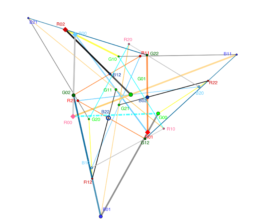
(a) Line $Z_{00}$ (dashed) is just above point $B_{22}$ (hollow)

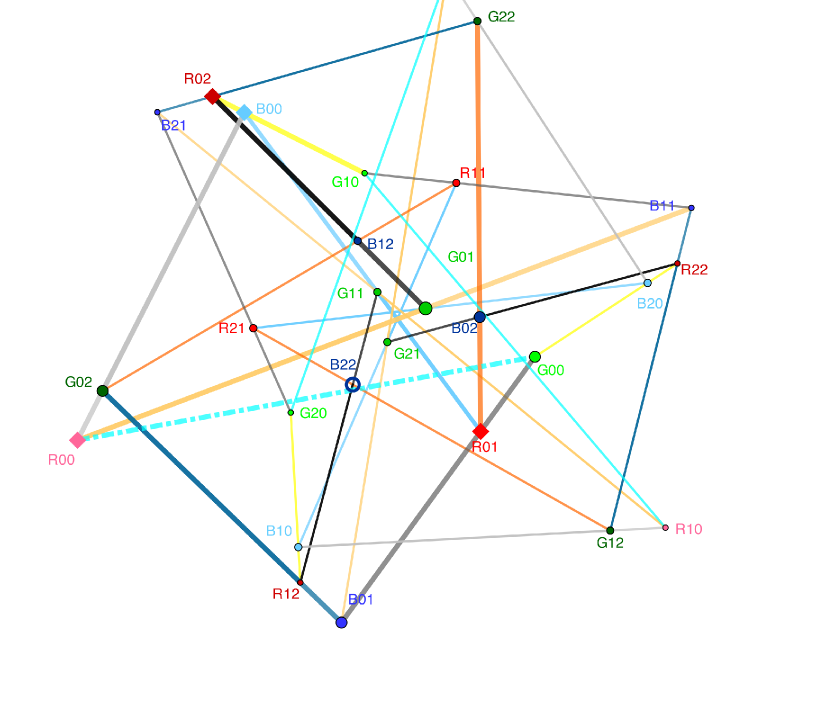
(b) Line $Z_{00}$ (dashed) is just below point $B_{22}$ (hollow)

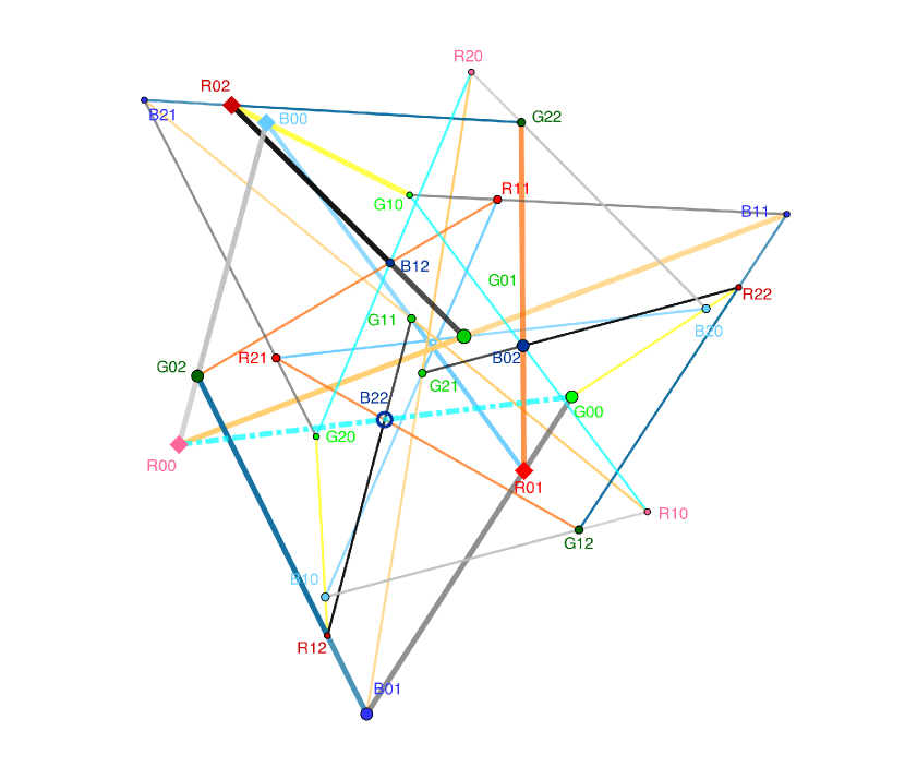
(c) The exact configuration, by continuity.

Figure 10: Realizing the Gray configuration with the Pappus RLG. The 0th element of each point and line class is shown larger/thicker. Points $R$, $G$, $B$ are shown in shades of red, green, blue respectively (going from light to dark as $j=0,1,2$) and similarly for line classes $X,Y,Z$ using shades of black, yellow, cyan. Points shown with diamonds are movable. (The movable lines are not specifically indicated.) Moving $R_{00}$ along its line moves the cyan dashed line $Z_{00}$ from above the point $B_{22}$ (shown hollow) to below the point $B_{22}$, so by continuity there is a position of $R_{22}$ in which line $Z_{00}$ passes through $B_{22}$ exactly. The $\mathbb{Z}_{3}$ action is counterclockwise rotation through $2\pi/3$ and corresponds to adding $+111$ to each point label.

6 A polycyclic realization of the Gray configuration with threefold rotational symmetry, using the $GG$ RLG.

A polycyclic realization of the Gray configuration with threefold rotational symmetry is depicted in Figure 11. The reduced Levi graph using $\mathbb{Z}_{3}$ as the voltage group is $GG$.

In what follows we explain how this realization is constructed.

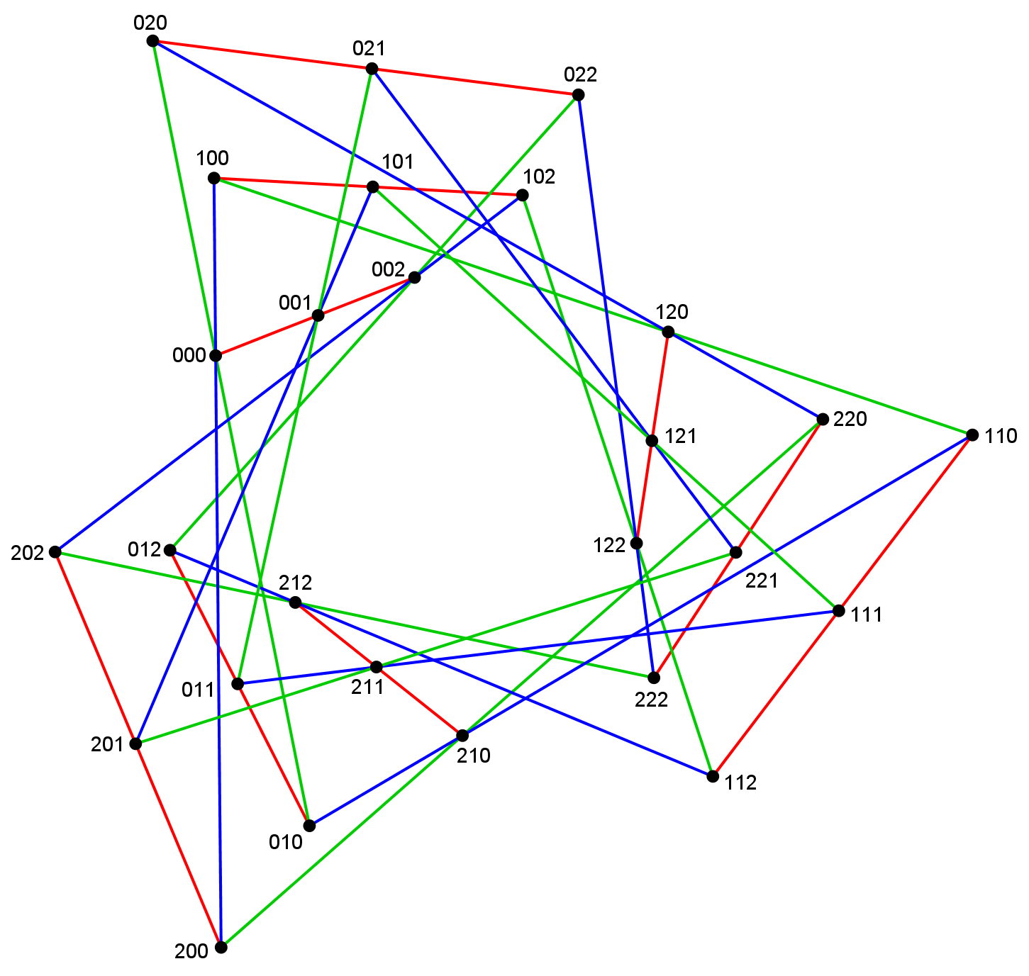
Figure 11: The Gray configuration: a polycyclic realization with 3-fold rotational symmetry. The labels of points are those introduced in Section 1. The colors emphasize resolvability of the configuration (show the parallel classes). Note that the $\mathbb{Z}_{3}$ action corresponds to adding $+210$ to each point label.

We start from a polycyclic realization of the Pappus configuration, see Figure 12. This realization is well known; it occurs e.g. in [17, Figure 1.16] and in [26, Figure 1.10]. The Pappus configuration contains as a subconfiguration the $(9_{2},6_{3})$ “grid” configuration, which is shown in Figure 12 by blue and green lines. The labels of the points in that figure verify that this is so, indeed (note that the third coordinate in these labels show that this configuration can be conceived as lying in the $XY$ plane of a spatial Cartesian coordinate system). This implies that using two additional suitable copies of the $(9_{2},6_{3})$ configuration (along with adding 9 independent lines), one obtains a realization of the Gray configuration given in Figure 11.

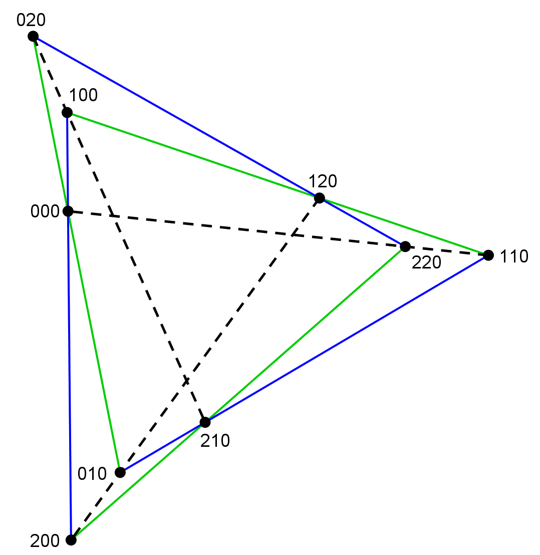
Figure 12: Polycyclic realization of the Pappus configuration with 3-fold rotational symmetry. Removal of the dashed lines gives rise to a polycyclic realization of the $(9_{2},6_{3})$ “grid” configuration.

To this end we need the following Theorem [22, 30].

Theorem 1.

Assume that a geometric figure $\mathcal{F}$ changes continuously in such a way that

1. precisely one of its points is fixed (denote it by $O$);

2. it is at all times directly similar to its original copy.

Consider two points $P,P^{\prime}\in\mathcal{F}$, both different from $O$. Then, if $P$ moves along a path $\ell$, then $P^{\prime}$ moves along a path $\ell^{\prime}$ such that $\ell^{\prime}$ is an image of $\ell$ under a dilative rotation.

Note that “directly similar” means that while changing $\mathcal{F}$, its orientation is preserved; in this procedure, images of $\mathcal{F}$ occur under the action of a one-parameter family of dilative rotations (also known as spiral similarities). For some properties of a dilative rotation, see e.g. [9].

We apply this theorem in the following way. Take a copy of a polycyclic realization of the $(9_{2},6_{3})$ “grid” configuration (let it be denoted by $\mathcal{G}_{0}$). Denote its centre of rotation by $O$, and fix this point; it plays the role of the point $O$ of the theorem. Choose a straight line which passes through a configuration point of this grid, but avoids all its other configuration points as well as the centre $O$; this will play the role of the path $\ell$ of the theorem, thus we shall refer to it by the same notation. Considering our Figure 11, the starting copy of the grid configuration can be taken as a copy of precisely what is depicted in Figure 12 (with the same labels of points). In addition, the line $\ell$ is taken as the red line through the point $(020)$.

Now take the copies $\mathcal{G}_{1}$ and $\mathcal{G}_{2}$ which are images of $\mathcal{G}_{0}$ under dilative rotations such that their points $(021)$ and $(022)$, respectively correspond to the point $(020)$, and lie on the line $\ell$. As a consequence of Theorem 1 above, we have that the points of the set $\mathcal{G}_{0}\cup\mathcal{G}_{1}\cup\mathcal{G}_{2}$ are arranged into collinear triples along the 9 red lines of our Figure 11 (note that all these lines are copies of $\ell$ under dilative rotations, again due to the theorem). As a result, the set $\mathcal{G}_{0}\cup\mathcal{G}_{1}\cup\mathcal{G}_{2}$, together with the 9 new lines, forms a configuration which is isomorphic to the Gray configuration; moreover, it is polycyclic with threefold rotational symmetry.

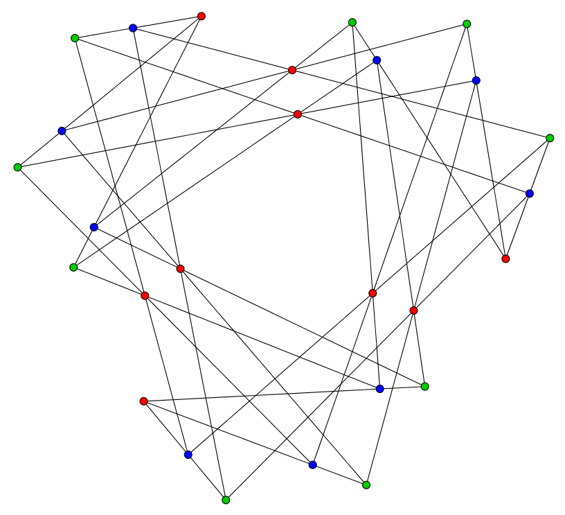
Figure 13: Using reciprocation on the configuration shown in Figure 11, we also construct a realization of the dual configuration to the Gray configuration.

Clearly, the realization of the Gray configuration shown in Figure 11 has 3-fold rotational symmetry, and it is easy to verify that the rotation corresponds to adding +210 to each of the point labels. We previously showed that adding +210 corresponds to the reduced Levi graph shown in Figure  8, so this realization is a polycylic realization with graph $GG$ as its reduced Levi graph.

This geometric realization has been used to construct a unit-distance realization of the Gray graph; see [4].

7 9-fold symmetry of the Gray Graph and Gray Configuration

7.1 9-fold symmetry of the Gray graph

Figure 14 shows two drawings of the Gray Graph with 9-fold rotational symmetry, which interact nicely with the Pappus realization. (The graph on the left has the positions of the rings of points and lines chosen so that the graph is intelligible, while the graph on the right has the $GG$ symmetry class elements lined up; there is no change in the order of the elements along each rotational ring, just in the position of the 0th element of each ring of points and of lines.) Specifically, 3-fold rotation preserves the symmetry classes under the Pappus action. For example, considering the class $B_{i0}=\{B_{00}=100,B_{10}=211,B_{20}=022\}$ shown in blue, located on the outermost ring of the graph, rotation by $120^{\circ}$ maps $B_{00}\to B_{10}\to B_{20}$. It is easy to verify that all of the Pappus symmetry classes (the color-coded columns in Table 2) are preserved by this 3-fold rotation.

Figure 14: Two drawings of the Gray Graph with $\mathbb{Z}_{9}$ symmetry. Note that the symmetry classes under the Pappus action (the columns in Table 2) are preserved under 3-fold rotation applied to this graph. The elements $*_{0j}$, $*\in\{X,Y,Z,R,B,G\}$ (that is, the first rows in Table 2) are shown thick.

Table 3 lists the symmetry classes of points and lines that correspond to this realization of the Gray Graph using $\mathbb{Z}_{9}$ symmetry, shown in Figure 14. They are chosen so that 3-fold rotation permutes the “Pappus” symmetry classes (that is, the colored columns in Table 2.

Table 3: Symmetry classes of points and lines corresponding to a $\mathbb{Z}_{9}$ realization of the Gray Graph.

symmetry point class $$D R_{00},B_{00},G_{00},R_{10},B_{10},G_{10},R_{20},B_{20},G_{20}$$:

$$= \ 000,100,110,111,211,221,222,022,002$$

symmetry line class $$L X_{00},Y_{00},Z_{00},X_{10},Y_{21},Z_{10},X_{20},Y_{20},Z_{20}$$:

$$= \ \!*\!00,1\!*\!0,11*,*11,2\!*\!1,22*,*22,0\!*\!2,00*$$

symmetry point class $$F R_{02},B_{22},G_{12},R_{12},B_{02},G_{22},R_{22},B_{12},G_{02}$$:

$$= \ 120,112,011,201,220,122,012,001,200$$

symmetry line class $$N X_{02},Y_{22},Z_{12},X_{12},Y_{02},Z_{22},X_{22},Y_{12},Z_{02}$$:

$$= \ \!*\!20,12*,01*,*01,2\!*\!0,12*,*12,0\!*\!1,20*$$

symmetry point class $$E R_{01},B_{11},G_{21},R_{11},B_{21},G_{01},R_{21},B_{01},G_{11}$$:

$$= \ 210,121,212,012,202,020,102,010,101$$

symmetry line class $$M X_{01},Y_{11},Z_{21},X_{11},Y_{21},Z_{01},X_{21},Y_{01},Z_{11}$$:

$$= \ \!*\!10,1\!*\!1,21*,*21,2\!*\!2,02*,*02,0\!*\!0,10*$$

The symmetry classes under the $GG$ action (the color-coded rows in Table 2) are preserved through interchanging the rings of symmetry classes, but the action is more complicated. Simply cyclically permuting the three rings (outside-middle-inside) in the second drawing in Figure 14 permutes the elements in the classes $R_{0i},R_{1i},R_{2i}$ and $X_{0i},X_{1i},X_{2i}$: for example, mapping the outer ring to the middle ring to the center ring applies the permutation $R_{00}=000\to R_{01}=210\to R_{02}=120$. However, the permuting of the rings does not map the other $GG$ symmetry classes to themselves directly. To preserve the classes $B_{ij}$ (blue) and $Y_{ij}$ (orange), $i=0,1,2$, permuting the rings plus a $-120^{\circ}$ rotation is required: for example, mapping the outer ring to the middle ring and rotating backwards by $120^{\circ}$ sends $B_{00}=100\to B_{01}=010$, and doing that action again sends $B_{01}=010\to B_{02}=220$. Similarly, to preserve $GG$ classes $G_{ij}$ (green) and $Z_{ij}$ (cyan), $i=0,1,2$, requires a ring permutation and a rotation by $+120^{\circ}$.

7.2 Constructing a $\mathbb{Z}_{9}$ realization

We use the 9-fold rotation of the graph shown in Figure 14 to construct orbits of length 9 of points and lines, listed in Table 3. The 0th element of each orbit is shown thick in Figure 14. These symmetry classes can be seen as 9-cycles on the standard grid, viewed as a solid torus formed by identifying opposite sides of the $3\times 3$ grid, shown in Figure 15. However, producing the symmetry classes listed in Table 3 is not as straightforward as just following the 9-gons. The sequence of points and lines obtained by following the solid 9-gon on the torus corresponds to alternating points in class $D$ and lines in class $L$. However, to alternate between $F$ and $N$ requires skipping 2 steps on the doubled 9-gon, and to alternate between $E$ and $M$ requires skipping 4 steps on the dashed 9-gon.

Figure 15: Identifying $\mathbb{Z}_{9}$ symmetry classes in the Gray Grid. Successive points in symmetry class $D$ occur by traveling one step along the solid black 9-gon, successive points in symmetry class $F$ occur by traveling two steps along the doubled 9-gon, and successive points in symmetry class $E$ occur by travelling four steps along the dashed 9-gon (in each case, following the direction of the arrows). The 0th element of each point class is indicated by a heavy circle.

Using the drawings in Figure 14, it is straightforward to read off the voltages for the $\mathbb{Z}_{9}$ voltage graph, shown in Figure 16(a). As usual, we then add and subtract voltages to produce a reduced Levi graph with a spanning path 16(b), to aid in applying known algorithms for constructing configurations with reduced Levi graphs of this type.

Figure 16(c) shows the corresponding drawing of the Gray Graph emphasizing the $\mathbb{Z}_{9}$ symmetry classes.

(a) The reduced Levi graph corresponding to the graphs shown in Figure 14. Thick edges correspond to labels of 0.

(b) Adding and subtracting voltages as necessary results in a $\mathbb{Z}_{9}$ voltage graph with a Hamiltonian spanning path of 0-labeled edges.

(c) The Gray graph viewed as the expanded Levi graph, emphasizing the spanning path of 0 indicated in the voltage graph (which can be seen following the “spine” of the graph, shown thick). As usual, points are circular nodes and lines are rectangular nodes.

Figure 16: Helpful realizations of the Gray graph and the $\mathbb{Z}_{9}$ voltage graph.

The voltage graph shown in Figure 16(b) is an example of a voltage graph that corresponds to a multilateral chiral 3-configuration, as described in [3] as a configuration whose reduced Levi graph over some $\mathbb{Z}_{m}$ is 3-regular and alternates double (parallel) arcs and single arcs. That paper provided an algorithm for constructing corresponding geometric configurations. The Configuration Construction Lemma, described in that paper and elsewhere, says, essentially, the following: Given a set of points $P_{i}$ that are cyclically labeled as the vertices of a regular $m$-gon centered at the origin $\mathcal{O}$, construct the circle $C$ passing through points $P_{b}$, $\mathcal{O}$, $P_{b-d}$. If a point $Q$ lies on $C$, and if $Q^{\prime}$ is the rotation of $Q$ by $\frac{2\pi d}{m}$, then the line $QQ^{\prime}$ passes through $P_{b}$. This is particularly useful if the point $Q$ is constructed as the intersection of some other line constructed in the configuration with the circle $C$. In this case, to realize the given reduced Levi graph, the required process is as follows:

Algorithm 2.

To construct a geometric realization of a 3-configuration with the reduced Levi graph in Figure 16(b), do the following (with index arithmetic modulo 9):

1. Construct points $D_{i}$, $i=0,1,\ldots,8$ as the vertices of a regular 9-gon; specifically, let $D_{i}=(\cos(2\pi i/9),\sin(2\pi i/9))$.

2. Construct lines $L_{i}=D_{i}D_{i+1}$;

3. Place a point $F_{0}(t)$ arbitrarily (parameterized by $t$) on line $L_{0}$ and let $F_{i}(t)$ be the rotation of $F_{0}$ through $2\pi i/9$ about the origin;

4. Construct lines $N_{i}(t)=F_{i}(t)F_{i+4}(t)$

5. Construct a circle $\mathcal{C}$ through the three points $D_{-1}$, $D_{-1-2}$ and the origin;

6. Construct point $E_{0}$ to be the intersection of line $N_{0}(t)$ with $\mathcal{C}$, if it exists. If no point of intersection exists, then the algorithm fails. If a point of intersection exists, let $E_{i}$ be the rotation of $E_{0}$ through $2\pi i/9$ about the origin;

7. Construct lines $M_{i}=E_{i}E_{i+2}$. The line $M_{i}$ will pass through the point $D_{i-1}$.

Theorem 3.

There are exactly two positions of $F_{0}(t)$ on $L_{0}$ so that the line $N_{0}(t)=F_{0}(t)F_{4}(t)$ intersects the circle $\mathcal{C}$ passing through the three points $D_{-1}$, $D_{-3}$ and $\mathcal{O}$. These two positions are precisely the points $P_{1}=L_{0}\cap L_{-3}$ and $P_{2}=L_{0}\cap L_{3}$, and at these positions, the line $N_{0}(t)$ is tangent to $\mathcal{C}$. For all other values of $t$, the line $N_{0}(t)$ does not intersect $\mathcal{C}$. Therefore, any straight-line realization of the Gray Configuration with $\mathbb{Z}_{9}$ symmetry is a weak realization, because there are extra incidences caused by the fact that $F_{0}$ lies on two lines $L_{i}$ (rather than only one).

To prove this theorem, we will use the following lemma:

Lemma 4.

Let $\ell$ be a line and let $\ell^{\prime}$ be the rotate of $\ell$ through some angle $\theta$ about a point $\mathcal{O}$. Let $P$ be an arbitrary point on $\ell$ and $P^{\prime}$ the rotate through $\theta$ about $\mathcal{O}$ of $P$ (thus $P^{\prime}$ lies on $\ell^{\prime}$). The envelope of the lines $\overline{PP^{\prime}}$ is a parabola with focus $\mathcal{O}$ and directrix formed by the line $\overline{O_{\ell}O_{\ell^{\prime}}}$, where $O_{\ell}$, $O_{\ell^{\prime}}$ are formed by reflecting $\mathcal{O}$ over $\ell$, $\ell^{\prime}$ respectively.

Proof.

Recall that to construct a parabola with a given focus and tangent to two given lines, the directrix is formed by reflecting the focus over each of those two lines and joining the image points. Let $\mathcal{P}$ be the parabola with focus $\mathcal{O}$ that is tangent to the lines $\ell$ and $\ell^{\prime}$. Using similar triangles and angle-chasing, it is straightforward to show that in the above situation, if we reflect $\mathcal{O}$ over the line $PP^{\prime}$ to form the point $O_{PP^{\prime}}$, the three points $O_{\ell}$, $O_{\ell^{\prime}}$ and $O_{PP^{\prime}}$ are collinear; thus, the variable line $PP^{\prime}$ is tangent to the parabola $\mathcal{P}$ for all choices of point $P$. In addition, if $M_{\ell}$, $M_{\ell^{\prime}}$ are the feet of the perpendiculars to $\ell$, $\ell^{\prime}$ passing through $\mathcal{O}$, the vertex $V$ of $\mathcal{P}$ is the midpoint of the segment $M_{\ell}M_{\ell^{\prime}}$, and the line $M_{\ell}M_{\ell^{\prime}}$ is tangent to $\mathcal{P}$ at $V$. ∎

Proof of Theorem 3.

Consider the setup of Algorithm 2, except for convenience, choose starting coordinates

$$D_{i}=\left(\cos\left(\frac{2\pi i}{9}+\frac{17\pi}{18}\right),\sin\left(\frac{2\pi i}{9}+\frac{17\pi}{18}\right)\right).$$

With this choice of coordinates, by Lemma 4, the lines $L_{0}$ and $L_{4}$ (which is the rotate of line $L_{0}$ through the angle $\theta=4\cdot\frac{2\pi}{9}$ about $\mathcal{O}$) are tangent to a parabola $\mathcal{P}$ with focus at $\mathcal{O}=(0,0)$ and axis of symmetry on the $y$-axis. Using basic trigonometry, it is straightforward to show that the directrix of $\mathcal{P}$ is parallel to the $x$-axis and has equation $y=-2\cos\left(\frac{2\pi}{9}\right)\cos\left(\frac{4\pi}{9}\right)$. See Figure 17 for labels and details.

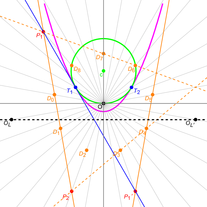
Figure 17: Illustrating the proof of Theorem 3. The circle $\mathcal{C}$ and its center are shown in green; the parabola $\mathcal{P}$ is shown in magenta with its directrix dashed black. The points $D_{i}$ and the lines $L_{0}$, $L_{4}$ are shown in orange, with $L_{-3}$ and $L_{3}$ shown in dashed orange. The points of tangency $T_{1}$ and $T_{2}$ between $\mathcal{P}$ and $\mathcal{C}$ are shown in blue, along with the line connecting $P_{1}$ and $P_{1}^{\prime}$ (shown in red) that passes through $T_{1}$. The thin gray lines mark out angles of $\frac{\pi}{18}$.

Since the general formula of a parabola that opens up, whose axis of symmetry is the $y$-axis, and whose focus at the origin is $x^{2}=4p^{2}+4py$, where $p$ is half the distance from the focus to the directrix, it follows that the parabola $\mathcal{P}$ has equation

$$x^{2} =4y\cos\left(\frac{2\pi}{9}\right)\cos\left(\frac{4\pi}{9}\right)+4\cos^{2}\left(\frac{2\pi}{9}\right)\cos^{2}\left(\frac{4\pi}{9}\right)$$

$$=4y\sin\left(\frac{\pi}{18}\right)\cos\left(\frac{\pi}{9}\right)+4\sin^{2}\left(\frac{\pi}{18}\right)\cos^{2}\left(\frac{\pi}{9}\right)$$

after simplification.

It is straightforward to show that the circle $\mathcal{C}$ passing through $D_{-1},D_{-3},\mathcal{O}$ has center $c=(0,\frac{1}{2\cos(2\pi/9)})$ and equation

$$x^{2}+y^{2}-y\sec\left(\frac{2\pi}{9}\right)=0.$$

Define $F_{0}(t)=(1-t)D_{0}+tD_{1}$ to be a variable point on line $L_{0}$, and define its rotate $F_{4}(t)=(1-t)D_{4}+tD_{5}$; that is, $F_{4}(t)$ is the rotate of $F_{0}(t)$ through $\frac{4\cdot 2\pi}{9}$ about $\mathcal{O}$. As in Algorithm 2, define $N_{0}(t)=F_{0}(t)F_{4}(t)$. By Lemma 4, this (generic) line $N_{0}(t)$ is tangent to $\mathcal{P}$. Thus, to investigate which lines $N_{0}(t)$ intersect $\mathcal{C}$, we can first investigate the intersections of the parabola and the circle.

Using Mathematica, we solve for the intersections of $\mathcal{C}$ and $\mathcal{P}$. No solutions would indicate that the circle and the parabola have no real intersections; four distinct solutions would indicate that the circle and the parabola intersect transversally; and two distinct solutions would show that the circle and the parabola intersect only at two tangent points. It is this third possiblity that turns out to be the case: after simplification, the only points of intersection between $\mathcal{P}$ and $\mathcal{C}$ are two points of tangency

$$T_{1} =\left(-2\sqrt{3}\sin\left(\frac{\pi}{18}\right)\cos\left(\frac{\pi}{9}\right),2\sin\left(\frac{\pi}{18}\right)\cos\left(\frac{\pi}{9}\right)\right)$$

and

$$T_{2} =\left(2\sqrt{3}\sin\left(\frac{\pi}{18}\right)\cos\left(\frac{\pi}{9}\right),2\sin\left(\frac{\pi}{18}\right)\cos\left(\frac{\pi}{9}\right)\right).$$

We claim that the tangent line to $T_{1}$ is precisely the line that passes through $P_{1}=L_{-3}\cap L_{0}$ and its rotate $P_{1}^{\prime}$ through $\frac{4\cdot 2\pi}{9}$ about $\mathcal{O}$. Elementary right-triangle trigonometry shows that the coordinates of $P_{1}$ and $P_{1}^{\prime}$ are

$$P_{1} =2\cos\left(\frac{\pi}{9}\right)\left(-\sin\left(\frac{2\pi}{9}\right),\cos\left(\frac{2\pi}{9}\right)\right)$$

$$P_{1}^{\prime} =2\cos\left(\frac{\pi}{9}\right)\left(\sin\left(\frac{\pi}{9}\right),-\cos\left(\frac{\pi}{9}\right)\right)$$

Computing $\det\begin{pmatrix}P_{1}&P_{1}^{\prime}&T_{1}\\ 1&1&1\end{pmatrix}$ and verifying, by Mathematica, that the determinant equals 0 shows that $P_{1}$, $P_{1}^{\prime}$ and $T_{1}$ are collinear. Since (by construction of $P_{1}^{\prime}$) the line $\overline{P_{1}P_{1}^{\prime}}$ is a member of the envelope of lines to the parabola, it follows that $\overline{P_{1}P_{1}^{\prime}}$ is tangent to $\mathcal{P}$ at the point $T_{1}$.

Symmetry of the construction shows that if we use $P_{2}=L_{0}\cap L_{3}$ as the starting point on line $L_{0}$, that the corresponding line $P_{2}P_{2}^{\prime}$ (with $P_{2}^{\prime}$ the rotate of $P_{2}$ through $\frac{4\cdot 2\pi}{9}$ about $\mathcal{O}$) is tangent to $\mathcal{P}$ at $T_{2}$.

In summary, there are precisely two points (namely, $P_{1}$ and $P_{2}$) on $L_{0}$ that can serve as the points $F_{0}(t)$ that have the property that the line $N_{0}(t)$ intersects $\mathcal{C}$ at some point $E_{0}$, following the labeling from Algorithm 2, namely $E_{0}=T_{1}$ if $F_{0}(t)=P_{1}$, or $E_{0}=T_{2}$ if $F_{0}(t)=P_{2}$.

However, each of these possible points $F_{0}(t)$ has the property that in addition to the line $L_{0}$ passing through them, another line $L_{i}$ also passes through them. ∎

Remark 3.

In fact, choosing either of these points as $F_{0}$ and completing Algorithm 2 (see Figure 18(a), which uses the points $D_{i}$ rotated back so that $D_{0}=(1,0)$) results in four points lying on each line and four lines passing through each point; the resulting incidence structure is actually the $(27_{4})$ celestial configuration $9\#(1,3;4,3;2,3)$) (see, e.g., [18, Section 3.7] for details on 3-celestial configurations, where they are called $3$-astral configurations). These extra incidences mean that the construction from Algorithm 2 produces only a weak realization of the Gray configuration.

A pseudoline realization of a configuration is a drawing of a configuration in which lines are allowed to “wiggle” but any two can intersect at most once. (In the projective plane, any two pseudolines intersect exactly once.) See, for example, [18, 2, 15]. Two pseudoline drawings (topological realizations) of the Gray Configuration with $\mathbb{Z}_{9}$ symmetry are shown in Figure 18. The left-hand figure indicates what the weak realization would be with straight lines, via the celestial configuration $9\#(1,3;4,3;2,3)$, but the extra incidences are avoided with pseudolines using semicircular paths around the unwanted vertices. Note this drawing was also shown in [21, Figure 3]; Theorem 3 shows that this configuration is the only straight-line (weak) realization possible of the Gray graph with $\mathbb{Z}_{9}$ symmetry. The right-hand figure shows a pseudoline realization in which two orbits of lines are straight, and the third orbit uses pseudolines consisting of circular arcs in the area shown.

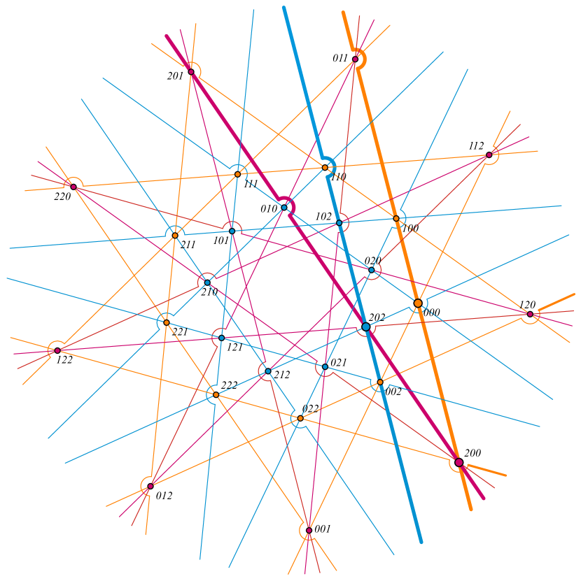
(a) A pseudoline drawing of the Gray configuration based on the $(27_{4})$ celestial configuration $9\#(1,3;4,3;2,3)$, avoiding the extra incidences with semicircles. Compare Figure 3 from [21].

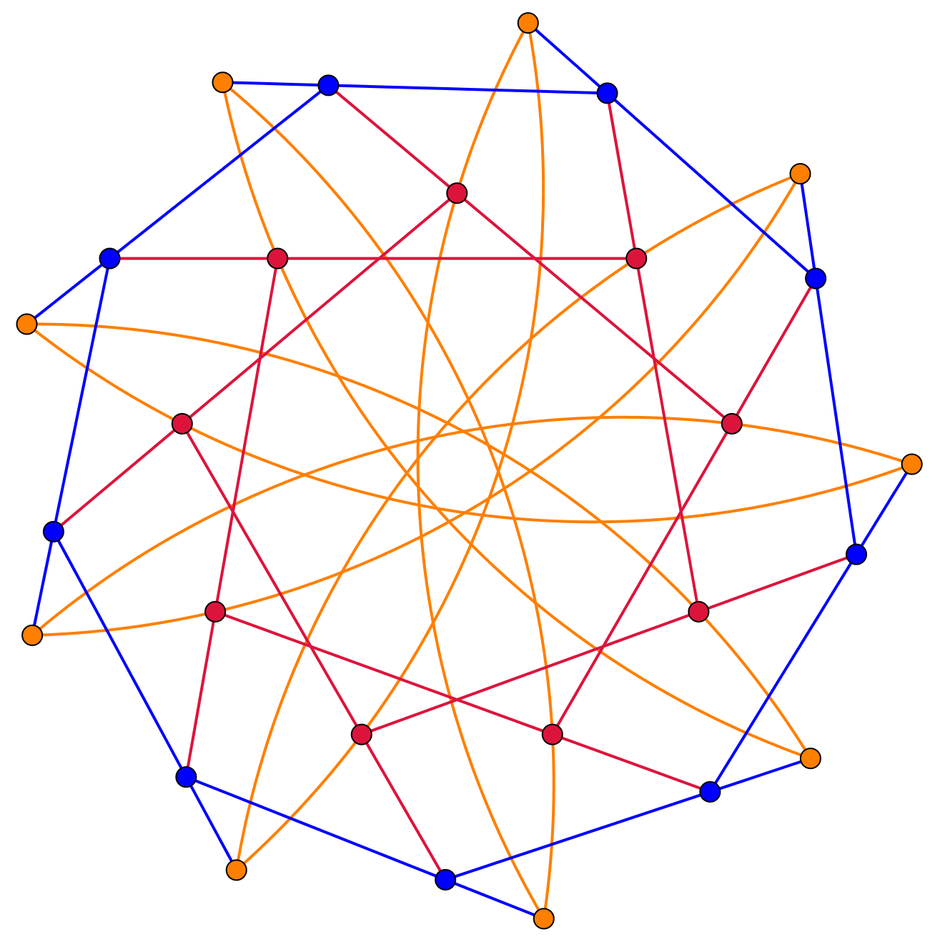
(b) A second pseudoline drawing, avoiding extra incidences.

Figure 18: Pseudoline realizations of the Gray configuration with $\mathbb{Z}_{9}$ symmetry.

8 Conclusion and open questions

We have showed that among all possible polycyclic realizations of the Gray configuration, it is possible to realize both $\mathbb{Z}_{3}$ versions, but the $\mathbb{Z}_{9}$ realization is only topological.

There are other semisymmetric cubic bipartite graphs of girth at least 6, including the Iofinova-Ivanov graph on 110 vertices (corresponding to a $(55_{3})$ configuration) [19]; the Ljubljana graph with 112 vertices (corresponding to a combinatorial $(56_{3})$ configuration [7]; the Tutte 12-cage, also known as the Benson Graph (corresponding to a combinatorial $(63_{3})$ configuration) with 126 vertices [1, 11]. A polycyclic geometric realization of the Ljubljana configuration with 7-fold symmetry was given in [7], and a polycyclic geometric realization of the configuration corresponding to the Tutte 12-cage has been shown in [5]. However, although [29] provides symmetric graph drawings, we are not aware of a published geometric realization of the Iofinova-Ivanov $(55_{3})$ configuration or its dual. We plan to investigate the geometric realizability of the corresponding configuration; the automorphism group of the graph is isomorphic to $\text{PGL}_{2}(11)$. Future work will explore the possibility of realizations of this configuration with 5-fold and 11-fold rotational symmetry.

Recently, Conder and Potočnik presented a method that enabled them to generate all semisymmetric cubic bipartite graphs of order up to 10000 [8]. It would be interesting if one could use our method with their census of examples to develop infinite families of geometrically realizable configurations.

References

- [1] Clark T. Benson. Minimal regular graphs of girths eight and twelve. Canadian J. Math., 18:1091–1094, 1966.
- [2] Leah Wrenn Berman. Symmetric simplicial pseudoline arrangements. Electron. J. Combin., 15(1):Research Paper 13, 31, 2008.
- [3] Leah Wrenn Berman. Geometric constructions for 3-configurations with non-trivial geometric symmetry. Electron. J. Combin., 20(3):Paper 9, 29, 2013.
- [4] Leah Wrenn Berman, Gábor Gévay, and Tomaž Pisanski. The Gray graph is a unit-distance graph. The Art of Discrete and Applied Mathematics, accepted, 2025.
- [5] Marko Boben, Branko Grünbaum, and Tomaž Pisanski. Multilaterals in configurations. Beitr. Algebra Geom., 54(1):263–275, 2013.
- [6] Izak Zurk Bouwer. On edge but not vertex transitive regular graphs. J. Combin Theory Ser. B., 12:32–40, 1972.
- [7] Marston Conder, Aleksander Malnič, Dragan Marušič, Tomaž Pisanski, and Primož Potočnik. The edge-transitive but not vertex-transitive cubic graph on 112 vertices. J. Graph Theory, 50(1):25–42, 2005.
- [8] Marston Conder and Primož Potočnik. Edge-transitive cubic graphs: Cataloguing and enumeration. https://arxiv.org/abs/2502.02250, 2025.
- [9] H. S. M. Coxeter and S. L. Greitzer. Geometry Revisited. The Mathematical Association of America, Washington, DC, 1967.
- [10] Ted Dobson, Aleksander Malnič, and Dragan Marušič. Symmetry in graphs, volume 198. Cambridge University Press, 2022.
- [11] Geoffrey Exoo and Robert Jajcay. Dynamic cage survey. Electron. J. Combin., DS16(Dynamic Surveys):48, 2008.
- [12] Jon Folkman. Regular line-symmetric graphs. J. Combin Theory, 3:215–232, 1962.
- [13] Gábor Gévay. Constructions for large spatial point-line configurations. Ars Math. Contemp., 7:175–199, 2013.
- [14] Gábor Gévay. Resolvable configurations. Discrete Appl. Math., 266:319–330, 2019.
- [15] Jacob E. Goodman, Joseph O’Rourke, and Csaba D. Tóth, editors. Handbook of discrete and computational geometry. Discrete Mathematics and its Applications (Boca Raton). CRC Press, Boca Raton, FL, 2018. Third edition of [ MR1730156].
- [16] Jonathan L Gross and Thomas W Tucker. Topological graph theory. Courier Corporation, 2001.
- [17] Branko Grünbaum. Connected configurations exist for almost all . Geombinatorics, 10(1):24–29, 2000.
- [18] Branko Grünbaum. Configurations of Points and Lines, volume 103 of Graduate Studies in Mathematics. American Mathematical Society, Providence, RI, 2009.
- [19] A. A. Ivanov and M. E. Iofinova. Biprimitive cubic graphs. In Investigations in the algebraic theory of combinatorial objects (Russian), pages 123–134. Vsesoyuz. Nauchno-Issled. Inst. Sistem. Issled., Moscow, 1985.
- [20] Dragan Marušič and Tomaž Pisanski. The Gray graph revisited. J. Graph Theory, 35:1–7, 2000.
- [21] Dragan Marušič, Tomaž Pisanski, and Steve Wilson. The genus of the GRAY graph is 7. Eur. J. Combin., 26:377–385, 2005.
- [22] Emil Molnár. Elemi matematika II. Geometriai transzformációk (Elementary Mathematics II. Geometric Transformations) (in Hungarian). Tankönyvkiadó, Budapest, 1990.
- [23] Barry Monson, Tomaž Pisanski, Egon Schulte, and Asia Ivić Weiss. Semisymmetric graphs from polytopes. J. Combin Theory Ser. A., 114:421–435, 2007.
- [24] Tomaž Pisanski. Yet another look at the Gray graph. New Zealand J. Math., 36:85–92, 2007.
- [25] Tomaž Pisanski and Milan Randić. Bridges between geometry and graph theory. In C. A. Gorini, editor, Geometry at Work, pages 174–194. Math. Assoc. America, Washington, DC, 2000.
- [26] Tomaž Pisanski and Brigitte Servatius. Configurations from a Graphical Viewpoint. Birkhäuser Advanced Texts. Birkhäuser, New York, 2013.
- [27] Gert Sabidussi. On a class of fixed-point-free graphs. Proc. Amer. Math. Soc., 9:800–804, 1958.
- [28] The Sage Developers. SageMath, the Sage Mathematics Software System (Version 9.6), 2022. https://www.sagemath.org.
- [29] Eric W. Weisstein. “Iofinova-Ivanov graphs.”. https://mathworld.wolfram.com/Iofinova-IvanovGraphs.html.
- [30] Isaak Moiseevich Yaglom. Geometric Transformations II. Random House, New York, 1968.