Bohmian Mechanics fails to compute multi-time correlations

Abstract

The violation of Bell type inequalities in quantum systems manifests that quantum states cannot be described by classical probability distributions. Yet, Bohmian mechanics is a realistic, non-local theory of classical particle trajectories that is claimed to be indistinguishable by observations from more traditional approaches to quantum mechanics. We set up a spatial version of the GHZ system with qubits realised as positional observables that demonstrates that the Bohmian theory fails to match predictions of textbook quantum mechanics (and most likely experients) unless enlarged by a microscopic theory of collapse of the wave function after observation. For this discrepancy to occur it is essential that positions at different times do not commute.

1 Introduction

The announcement of the 2022 Nobel Prize in Physics to Alain Aspect, John Clauser and Anton Zeilinger for the experimental demonstration of the violation of Bell type inequalities has sparked another round of arguments of what this actually implies for quantum theory.

In particular supporters of the Bohmian approachDuerr instited that by no means hidden variable theories are ruled out as their example of a hidden variable theory (with the Bohmian particle positions playing the role of the hidden variables) reproduces all the experimental predictions of more traditional approaches to quantum mechanics. It does this at the price of being non-local. Some have even argued that the Bell violation implies that quantum mechanics has to be a non-local theory.

In this note, we will examine this claim that the Bohmian theory matches all predictions of traditional quantum mechanics in more detail. To this end, we will study a version of the GHZ experiment (in the version popularized by Mermin and Coleman mermin ; coleman ) which is close in spiri to the Bell inequality but has the advantage of making definite statements instead of giving probabilities for measurement outcomes. We will, however, not formulate it in terms of spin degrees of freedom but rather use simple positional observables. Those are much better suited to a Bohmian description as the Bohmian theory in its original form posits all measurements in the end are measurements of positions: These can be positions of a pointer on a scale or in the case of spin degrees, positions of particles for which a spin degree has been translated in terms of a Stern-Gerlach-type experiment to a trajectory. By directly working with positional observables, we evade the complication of having to include the Stern-Gerlach set-up in our description including a Hamiltonian and an explicit solution for a time dependent wave function.

In order to realize the violation of the quantum inequalities, one has to make use of entanglement which in turn requires non-commuting observables. This seems to be in conflict with considering only position observables. But this can be circumvented by measuring positions at different instances of time as postions at different times are no longer required to commute. It is important though that the measurements at the different times are with respect to different particles or degrees of freedom and thus we do not attempt to measure complementary variables. It is only that for each degree of freedom we have the freedom to choose the time of measurement and different times correspond to observables that do not commute. But we always only choose one of those possibilities.

What we find is that the Bohmian approach fails to reproduce the expected results unless earlier observations influence later ones by the equivalent of a collapse of the wave function. After the first observation of one particle, the other Bohmian particles have to move with respect to a collapsed wave function rather than the original one. Thus, in order to be predictive, there has to be a quantitative understanding of this collapse process which is not in sight. The claim of equivalence of the two approaches can only hold in a Bohmian theory that is augmented by a mechanism that leads to a collapsing wave function. To be able to make quantitative predictions (that can be compared to the concrete predictions of more conventional approaches to quantum mechanics) it is not enough to simply state that some sort of collapse happens (or that somehow the wave function of the measuring device influences the system) but concrete equations of motion have to be supplied. If the collapse is not to be simply postulated in an ad hoc way, a microscopic mechanism for such a collapse is needed.

2 Setting the stage

Key to the Bohmian description of quantum mechanics is the conservation of the probability current for Hamiltonians of the form

$$H=-\sum_{i=1}^{N}\frac{1}{2m_{i}}\frac{\partial^{2}}{\partial x_{i}^{2}}+V(x_{1},\ldots,x_{N})$$

for a system with $N$ degrees of freedom where $m_{i}$ is the mass of the $i^{\rm th}$ degree of freedom. Dividing the probability current by the probability density leads to a velocity field

$$v_{i}(t;x_{1},\ldots,x_{N})=\frac{j_{i}(t,x_{1},\dots,x_{N})}{|\psi(t,x_{1},\ldots,x_{N})|^{2}}=\frac{1}{m_{i}}\Im\left(\frac{\partial\psi(t;x_{1},\ldots,x_{N})}{\partial x_{i}}\Big{/}\psi(t,x_{1},\ldots,x_{N})\right).$$

The de Broglie-Bohm theory posits now microscopic particles with positions $q_{i}(t)$ that follow the flow of this velocity field:

$$\frac{dq_{i}}{dt}=v_{i}(t;q_{1}(t),\ldots,q_{N}(t)).$$ (1)

If at time zero, these particles are distributed according the probability density

$$|\psi(0,x_{1},\ldots,x_{N})|^{2}$$

they will, thanks to the conservation of the probability current, be so at any other time as well. Thus, if all one is interested in are the distribution of the positions of particles (which is argued is all one would ever measure), the particle distribution of these microscopic particles is as predicted by traditional quantum mechanics.

It is important to realize though that the guiding equation (1) is non-local in the sense that the velocity of degree of freedom $i$ depends on the values of all other degrees of freedom, even if these are the coordinates of different particles that can be at arbitrarily large spatial separation. This non-locality is usually invoked in order to avoid the conclusions of Bell’s theorem as that assumes a local theory in the first place. Without locality, the outcome of a measurement on one particle can, at least in principle, depend on the settings of all detectors in the experiment. Our analysis will show, however, that this non-locality is not sufficient to produce the correlations in the GHZ experiment.

The positions $q_{i}(t)$ are the “realistic” state in the sense that the particles are objectively “there” even when not observed like for example the true microstate of a (classical) gas when only a macroscopic state is prescribed.

On the other hand, Bell’s inequality (and the likes like the GHZ experiment we are concerned with here) are derived assuming a local, realistic theory. Their violation in the quantum theory thus shows that the quantum world cannot be both local and realistic.

The GHZ system is tri-partite. On each of the three sub-systems (which can be thought of as separated by an arbitrarily large spatial distance) there are two possible measurements both with outcomes either $+1$ or $-1$. We will denote these two measurements of sub-system $a$ (and in slight abuse of notation also the outcome and later the corresponding observable) $X_{a}$ and $Y_{a}$ and similarly for sub-systems $b$ and $c$.

The whole GHZ experiment is repeated over many rounds. In the beginning of each round, the tri-partite system is prepared in the same particular “GHZ-state”. Then the three experimentators at the sub-systems randomly pick which of the two possible measurements they will conduct. They do the observation and write down which measurement they performed and the $\pm 1$ outcome.

Later, they compare their results. They find the outcomes of individual measurements to be random with vanishing expectation. Also all correlations of two of the measurements at two sub-systems are found to vanish. But there are non-trivial correlations when all three measurements are taken into account: They find that if they all did the $X$ measurement the product of the outcomes was always $-1$:

$$X_{a}X_{b}X_{c}=-1$$ (2)

In the case of one experimentator measuring $X$ and the other two operators measuring $Y$ the product is always $+1$:

$$X_{a}Y_{b}Y_{c}=Y_{a}X_{b}Y_{c}=Y_{a}Y_{B}X_{c}=+1$$ (3)

Since all outcomes are $\pm 1$, these equations can also be written as

$$X_{a}=Y_{b}Y_{c}\qquad X_{b}=Y_{a}Y_{c}\qquad X_{c}=Y_{a}Y_{b}.$$ (4)

In other words, if the measurements measure actual, preexisting properties of the sub-systems (i.e. that we are dealing with a realist theory), we can conclude that in the original state the $X$-property of one sub-system is determined by and can be deduced by the $Y$-properties of the other two sub-systems.

But taking the product of these equations one finds

$$X_{a}X_{b}X_{c}=(Y_{a}Y_{b}Y_{c})^{2}=+1,$$ (5)

In clear conflict with (2): Let’s assume both $X_{a}$ and $X_{b}$ both measure $+1$. Then (2) implies that $X_{c}$ has to be $-1$ while (5) impies that $X_{c}$ at the same time has to be $+1$.

This contradictions seems to make any such experiment with this type of correlations of outcomes impossible, at least in a local theory. The physical property that $X$ measures (which we will identify with particle positions below) cannot be both anti-correlated (as suggested by (2)) and correlated (as suggested by taking the three permutations of (3 into account) at the same time. In a non-local theory, however, the three sub-systems can “know” which of the measurements are conducted on the other sub-systems and adjust their outcome accordingly.

Quantum mechanically, by making use of entanglement it is possible to evade the impossibility: For example, one can assume the subsystems contain a qubit each and the $X$ and $Y$ measurements are the corresponding Pauli spin operators:

$$X=\begin{pmatrix}0&1\\ 1&0\\ \end{pmatrix}\qquad Y=\begin{pmatrix}0&i\\ -i&0\\ \end{pmatrix}$$ (6)

For the initial state, GHZ take

$$\Psi_{GHZ}=\frac{1}{\sqrt{2}}\big{(}|\uparrow\uparrow\uparrow\rangle-|\downarrow\downarrow\downarrow\rangle\big{)}$$ (7)

Applying $X$ to all three qubits flips them and $\Psi_{GHZ}$ is clearly an eigenstate of eigenvalue $-1$. Applying one $X$ and two $Y$-operators adds two factors $(\pm i)^{2}=-1$ in addition to the flip and thus $\Psi_{GHZ}$ is a $+1$ eigenstate of $X_{a}Y_{b}Y_{c}$, $Y_{a}X_{b}Y_{c}$, and $Y_{a}Y_{B}X_{c}$.

One (in this authors opinion: the) way to reconcile quantum theory with the above derivation of (5) is to give up realism: Since $X$ and $Y$ do not commute, they are complimentary variables that cannot both be measured at the same time on the same sub-system. Thus in a calculation involving $X_{a}$, it is not valid to assume that $Y_{a}$ has any (unknown but somehow objectively existing) value and similar for the other two sub-systems. So it is not legitimate to write an expression for $X_{a}X_{b}X_{c}$ that involves the $Y$’s since $Y_{a}$ fundamentally cannot be measured as well besides $X_{a}$ and thus one must not assume they still have a value. This is the local but non-realist way to explain the observed quantum correlations that appear to be impossible in a classical (and thus realist) theory.

The Bohmian theory goes in a different direction: There one insists on realistic degrees of freedom (the $q_{i}$’s) but is willing to give up locality. In this note, we will investigate how this is supposed work in detail and if the conflict between (2) and (5) is resolved in the Bohmian theory.

3 The Bohmian GHZ

Even though there is a version of the Bohm theory that can handle spin degrees of freedom, following the mantra of “all measurements in the end measure positions” one is supposed to run those through a Stern-Gerlach apparatus or similar to translate spin states into postion states. This complicates the analysis significantly since it means one has to take into account the Stern-Gerlach apparatuses in the systems Hamiltonian and guiding equation.

It is even arguedops1 ; ops2 that the only true properties of particles are their positions while spin is rather a property of the wave function and the observed value depends on the details of the experiment that is supposed to measure it. This explicitly allows for contextualism in the way that the result of the spin measurement on one particle (in terms of a Stern-Gerlach apparatus) depends on which spin component of a different particle is measured (in terms of setting up another Stern-Gerlach apparatus). After all, according to ops1 ; ops2 , only positions $q_{i}$ re both real and measurable.

But after all, all that the above description really needs are binary outcome observables $X$ and $Y$ that fulfil the required commutation relations. Two state systems are abundant also in spatial systems. But non-commuting observables might seem impossible to obtain if all one is allowed to use are multiplication operators in position representation. One can even speculate that restriction to such commuting position operators is what makes it possible for a theory that contains realistic particle orbits to behave like quantum theory.

Still, it is possible to avoid this restriction taking into account time evolution as positions at different times no longer commute. Specifically, we are going to use a set-up similar to what was used in bohmianangels which was inspired by werner ; CorreggiMorchio . A related situation with two time correlations was also investigated by Gisin in Gisin as well as laloe ; neumaier .

Let each sub-system consist of a particle in a box which we take to be the interval $[-\pi/2,\pi/2]$ and thus the Hilbert space as $L^{2}([-\pi/2,\pi/2])$ with the Hamiltonian of the free particle $H=-\frac{d^{2}}{dx^{2}}$ where we have set all masses $m_{i}=1/2$ for simplicity. We impose Dirichlet boundary conditions. We focus our attention to the ground state and the first excited state

$$g(x)=\sqrt{2/\pi}\cos(x)\qquad e(x)=\sqrt{2/\pi}\sin(2x)$$ (8)

with respective energies $E_{g}=1$ and $E_{e}=4$. In this system, we ask if the particle is in the left or in the right half of the interval which corresponds to the observable given by the multiplication operator by $\sigma(x)=\hbox{sgn}(x)$ which is $-1$ in the left half and $+1$ in the right half, see Fig. 1.

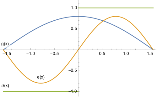
Figure 1: Wave functions of ground state and first excited state as well as $\sigma$

Since $g(x)$ is an even function while $e(x)$ and $\sigma(x)$ are odd, the expectation of $\sigma$ in both states vanishes

$$\langle g|\sigma|g\rangle=\langle e|\sigma|e\rangle=0,$$ (9)

but there is a non-trivial overlap

$$\langle g|\sigma|e\rangle=\frac{8}{3\pi}\approx 0.85$$ (10)

This was all at the initial time $t=0$. As they are energy eigenstates, $|g\rangle$ and $|e\rangle$ simply time evolve with a phase, so we have

$$\langle g|e^{-iHt}\sigma e^{iHt}|e\rangle=\frac{8}{3\pi}e^{i\Delta Et}$$ (11)

In the sector spanned by these two states, the $\sigma$-operator in the Heisenberg-picture $\sigma_{t}=e^{-iHt}\sigma e^{iHt}$ becomes

$$\sigma_{t}=\frac{8}{3\pi}\begin{pmatrix}0&e^{i\Delta Et}\\ e^{-i\Delta Et}&0\\ \end{pmatrix}.$$ (12)

So, up to a numerical factor, $\sigma_{0}$ plays the role of $X$, the Pauli spin matrix in the $x$-direction while $\sigma_{\pi/(2\Delta E)}$ is $Y$, the spin matrix in the $y$-direction. We have found a convenient set of non-commuting observables.

We can now set up the analogue of the GHZ-state: We use three copies of the the particle in a box $L^{2}([-\pi/2,\pi/2])\otimes L^{2}([-\pi/2,\pi/2])\otimes L^{2}([-\pi/2,\pi/2])\cong L^{2}([-\pi/2,\pi/2]^{3})$. This system can equivalently be viewed as three particles confined to three separate intervals (which can be thought of as located at large spatial separation) or alternatively as one particle in a three-dimensional box.

We set

$$\Psi_{GHZ}=\frac{1}{\sqrt{2}}\left(g\otimes g\otimes g-e\otimes e\otimes e\right)$$ (13)

or

$$\Psi_{GHZ}(x,y,z)=\frac{1}{\sqrt{2}}\left(g(x)g(y)g(z)-e(x)e(y)e(z)\right)$$ (14)

Different from the state considered in bohmianangels , $\Psi_{GHZ}$ is not stationary with respect to the free particle time evolution. The time evolution of the probability density is shown in Fig. 2.

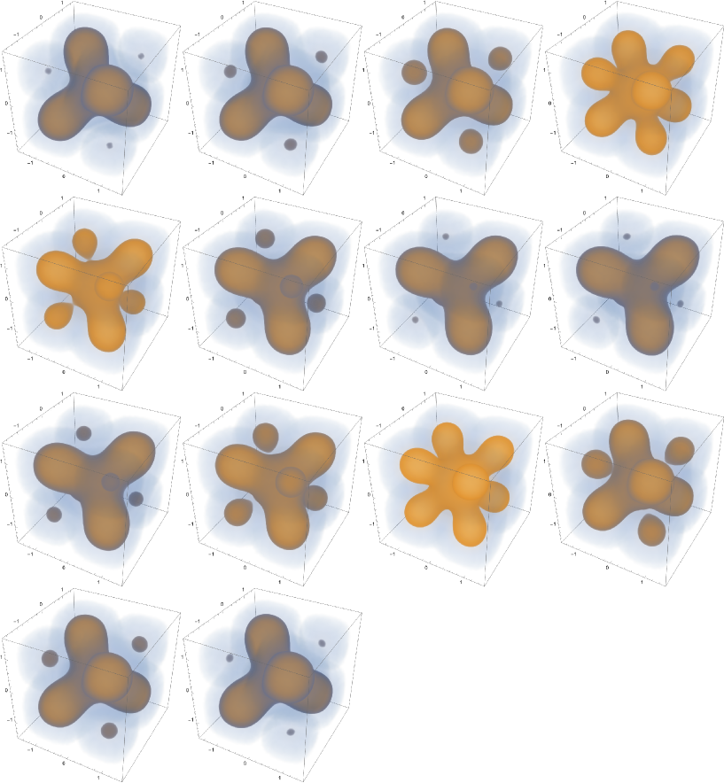
Figure 2: A comic of the periodic time evolution of the probability density $|\Psi_{GHZ}|^{2}$ as a particle in a three-dimensional box

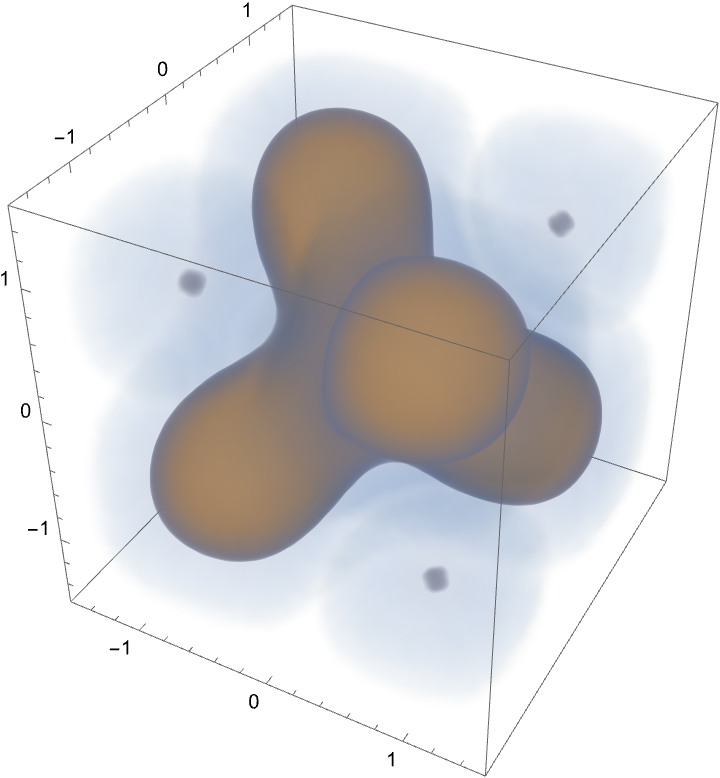
Figure 3: Propability distribution at $t=0$ and $t=\pi/(2\Delta E)$

At $t=0$ (Fig. 3), we can ask if the three particles are in the left or the right half of the interval. What is apparent from the probability distribution Fig. 3 can also be computed:

$$\langle\Psi_{GHZ}|\sigma\otimes\sigma\otimes\sigma|\Psi_{GHZ}\rangle=-\left(\frac{8}{3\pi}\right)^{3}$$ (15)

Up to a numerical factor, this is nothing but (2) in this positional setting. In other words, the initial probability distribution of the Bohmian positions as implied by $\Psi_{GHZ}$ has a strong anti-correlation: In the language of a particle in a three-dimensional box, the majority of the probability is in four out of the eight possible octants.

Similarly, we can do this at times $s$, $t$ and $u$ for the respective particles. A short calculation shows

$$\langle\Psi_{GHZ}|\sigma_{s}\otimes\sigma_{t}\otimes\sigma_{u}|\Psi_{GHZ}\rangle=-\cos(\Delta E(s+t+u))\left(\frac{8}{3\pi}\right)^{3}.$$ (16)

In particular, to find the expression corresponding to (3), we evaluate this for two times taken to be at $\pi/(2\Delta E)$ and the last one at $0$ (our set-up is of course invariant under permutations of the three particles):

$$\langle\Psi_{GHZ}|\sigma_{\pi/(2\Delta E)}\otimes\sigma_{\pi/(2\Delta E)}\otimes\sigma_{0}|\Psi_{GHZ}\rangle=+\left(\frac{8}{3\pi}\right)^{3}.$$ (17)

So picking any two of the three particles, compared to the initial position at $t=0$, exactly one of the pair has to have changed the side in the box at time $\pi/2\Delta E$. Of course, this is not possible for all possible pairs of two out of three particles!

So, up to a fidelity factor of $(8/3\pi)^{3}$, we recovered the situation of the GHZ experiment: From the three possible correlations of the positions of one particle at time zero with the two other particles at time $\pi/(2\Delta E)$, we would conclude by the same argument that lead to (5) that more likely the product of the signs of the positions of the three particles at the initial time is positive while it is actually negative.

Or put differently: The correlation (16) is not reproduced by the positions $q_{i}$ of the Bohmian particles if they evolve according the the evolution (1). On the other hand, anything else would have been surprising as the position of a particle would have to be both on the left as well as the right half of the interval depending on if one argues in analogy to (2) or (5). That is of course impossible for “objective” particle positions.

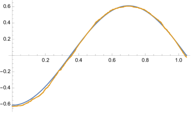
Figure 4: (16 (blue) for $t=s=u$ and the Bohmian expression $\mathbb{E}\langle\operatorname{sgn}(q_{1}(t))\operatorname{sgn}(q_{2}(t))\operatorname{sgn}(q_{3}(t))\rangle$ (orange) agree well

To strengthen this claim, we picked 1000 sets of initial positions from the probability distribution $|\Psi_{GHZ}|^{2}$ and numerically integrated the guiding equation (1) using mathematica. In the special case $s=t=u$ where the positions of the three particles are evaluated at identical times and the corresponding observables thus commute, we find excellent agreement with the expression (16) as shown in Fig. 4.

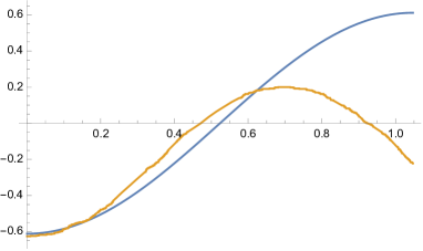
Figure 5: (16) for $t=0$ and $s=u$ (blue) and the Bohmian expression for the particles $\mathbb{E}\langle\operatorname{sgn}(q_{1}(0))\operatorname{sgn}(q_{2}(s))\operatorname{sgn}(q_{3}(s))\rangle$ (orange) no longer agree

If, however, we evaluate the position of one particle at the initial time $t=0$ the other two particles’ position at $s=u$, the Bohmian expression no longer agrees with (16) as is clear from Fig. 5. We find that correlations of the $q_{i}$ at different times do no longer agree with predictions for correlations of the corresponding Heisenberg picture observables. Positions at different times are not covered by the general “the Bohmian particle positions are distributed according to $|\psi|^{2}$ at every time and thus the pilot wave theory automatically reproduces all predictions of traditional quantum mechanics” explanation.

Even the non-local nature of the guiding equation is not able to reconcile the particle positions with the quantum theory predictions.

4 Ways out

There is, however, a way to save the Bohmian theory from this discrepancy and give it a chance to reproduce the conventionally computed result (which we strongly believe would be confirmed experimentally). We leave it to the reader to judge by how much this weakens the explanatory power of the Bohmian predictions.

This route starts with the realisation that it is not sufficient to ask where the three particles “are” at the given points in time (which would be expressed by the $q_{i}$ as they are supposed to be thought as the actual particle positions that would for example blacken exactly one silver grain on a photographic plate) but that it would have to be actually measured. But each measurement is known to disturb a quantum system.

We should point out that in the literatureops1 ; ops2 on Bohmian mechanics it is stressed that the Bohmian theory of trajectories is concerned with “what is really the case” not just with what some complicated apparatus is supposed to show. In fact, the focus of other approaches on observables is frowned upon since observables and measurements require an observer and thus introduce a subjective notion (what actually constitutes an observer?) into the discussion. The Bohmian theory in contrast claims to be about quantum theory without observers.

But leaving this attitude that has potential to challenge the nature of physics being an empirical theory (where certain notions like the particle positions $q_{i}$ are claimed to exist while at the same time are denied to be empirically accessible), one can entertain the idea that “where are the three particles at different times?” is not the right question but rather “where can I measure the particles at different times?”. In Gisin , after a similar analysis, Gisin proposes to give up what he calls “Hypothesis H” which states the strong connection between the Bohmian particle positions and the outcome of position measurements. This conclusion, however, severs the the Bohmian position variables completely of empirical content.

So if one decides to measure the position $q_{1}$ of the first particle at $t=0$, from that point on, one should no longer expect that the other two particles follow the guiding equation derived from $\Psi_{GHZ}(t)$ but rather from a collapsed wave function. Or said differently, because of its non-local nature, the guiding equation is not supposed to be applied to sub-systems, only to the wave function of the entire universe which not only contains the three particles with their postions but at least the measurement device used to detect the position $q_{1}$ of the first particle at $t=0$. Taking this seriously, however, means one can never be sure what the actual guiding equation is unless one has control over all degrees of freedom in the universe. There are no decoupled or approximate sub-systems and the predictability of the theory in any realistic situation is in doubt. Anybody who wants to argue along these lines should provide a calculation within the Bohmian framework which is able to reproduce the blue curve in Fig. 5 which is an experimentally testable prediction of the orthodox theory. The failure to compute this curve or the the claim that the outcome depends on further so far unspecified details of the experimental set-up constitute a lack of predictable power of the theory.

But this seems to be the view at least of some supporters of the Bohmian theory, at least that is our understanding of discussions in social media.

Another problem for a Bohmian model of a measuring device is that only the guiding equation (1) is sourced by the wave function but on the other hand there is no feedback from the particle positions $q_{i}(t)$ on the wave function which evolves according to the Schrödinger equation independently of the $q_{i}(t)$. So no detector wave function can depend on the $q_{i}$ of the measured particles. So within the Bohmian theory, it is not possible to describe dynamics of a measuring device which picks up the “actual positions” of the particles that it is supposed to measure. The observation of the values $q_{i}(t)$ can only happen outside of the Bohmian description.

It is important to stress that for other physical theories it is not the case, that since “everything is connected with everything”, it is impossible to make predictions for the correlations of the positions of the three particles at different times without detailed knowledge of the detection mechanism. In fact, standard quantum mechanics makes these predictions (16) for this system without additional knowledge of the microscopic details of the measuring device. So to match those predictions, the physics (as far as relevant for these predicted outcomes) must not depend on those details of the measuring device: Only one outcome can be correct, that one that matches the predictions of standard quantum mechanics.

Alternatively, one could try to implement some sort of collapse in the moment where the position of the first particle is detected. One has to throw away those possible paths $q_{i}(t)$ that are not compatible with the measurement and from the time of the measurement use a collapsed wave function

$$\frac{P\Psi_{GHZ}}{\|P\Psi_{GHZ}\|}$$

in the guiding equation where $P$ is the projector on the eigen-space of the measured observable (with unclear meaning in the case of continuous spectrum).

In any case, more detailed information (the form of the correct projector $P$ above) is required in order to obtain an updated guiding equation after the collapse in order for the theory to be able to reproduce the relatively easy prediction (16) which is independent of of microscopic details of the measurement process.

There is yet another logical possibility one can entertain to avoid the discrepancy pointed out above: That is that the particle positions observed are not the $q_{i}$ but rather something else, some property only of the wave function and the measurement device and independent of the $q_{i}$. But seriously entertaining this possibility takes out these “true particle positions” of any empirically founded scientific theory.

In conclusion it appears that the current situation is that in set-ups such as those discussed in this paper involving more than one instant of time either the predictions of the Bohmian particle positions are incompatible with standard expectations or there are no reliable predictions pending additional microscopic information or alternatively detailed knowledge of all degrees of freedom in the entire universe. The statement “the Bohmian theory trivially makes the same predictions as standard quantum mechanics because the positions of all particles are distributed according to the quantum mechanical probability distribution at all times” seems to not be a complete description in any case. This statement is only true if all measurements are supposed to happen at the same time. But even if one is happy with the “all measurements are position measurements after all, possibly of a pointer” there is no justification for only restricting to instantaneous measurements. And without this assumption not only there is no basis for the claim that the Bohmian positions agree with the $|\psi|^{2}$ distribution and thus with any other interpretation. In fact, in this note we show this is manifestly wrong.

On the other hand, a restriction only to position variables at a single instance of time would be a severe restriction that reduces quantum physics to a subsector (a commutative subalgebra) which lacks quantum properties as its states can be identified with classical probability distributions (thanks to the Gelfand-representationGelfand ).

In any case, the system presented here makes quantitative predictions in the conventional description which could easily be tested in an actually possible (not just speculative and potentially impossible) experiment which at best is a challenge for the Bohmian theory to reproduce and for which a straight forward application of the guiding equation and the identification of the $q_{i}$ with observable particle positions yields a quantitatively different prediction as shown in Fig. 5.

5 Appendix: Frauchinger-Renner states

A similar argument (although slightly more complex in the technical details) can be made for a state like that investigated by Frauchinger and RennerFR (for an analysis from the point of view of the Bohmian theory see LH ).

Here, we are dealing with two two-state systems. For the two-state Hilbert space we use a basis $\downarrow/\uparrow$ or alternatively $\leftarrow=(\downarrow-\uparrow)/\sqrt{2}$ and $\rightarrow=(\downarrow+\uparrow)/\sqrt{2}$ as well as $\circlearrowleft=(\uparrow+i\downarrow)/\sqrt{2}$ and $\circlearrowright=(\uparrow-i\downarrow)/\sqrt{2}$.

On the bipartite system, we prepare the state

$$\Psi_{FR} = \frac{\circlearrowright\otimes\circlearrowleft+(1+i)\circlearrowleft\otimes\leftarrow}{\sqrt{3}}$$

$$= \frac{\circlearrowleft\otimes\circlearrowright+\circlearrowright\otimes\circlearrowleft+i\circlearrowleft\otimes\circlearrowleft}{\sqrt{3}}$$

$$= \frac{(1-i)\leftarrow\otimes\circlearrowright+(1+i)\rightarrow\otimes\circlearrowright+2(1+i)\leftarrow\otimes\circlearrowleft}{\sqrt{12}}$$

$$= \frac{3\leftarrow\otimes\leftarrow+i\rightarrow\otimes\leftarrow+i\leftarrow\otimes\rightarrow+\rightarrow\otimes\rightarrow}{\sqrt{12}}$$

From the third line, one can conclude that if one measures the first particle in the state $\rightarrow$ the second particle will always in the state $\circlearrowright$. From the second line, one can conclude that if one however measures the second particle in the state $\circlearrowright$ the first particle has to be in the state $\circlearrowleft$. Finally, if one however measures the first particle in the state $\circlearrowleft$ the second particle will always be in the state $\leftarrow$ as can be seen from the first line.

It would be tempting to combine these three observations to come to the wrong conclusion that the combination $\rightarrow\otimes\rightarrow$ will never be realised but the fourth line shows that in fact it will be found in $1/12$ of the cases when measuring both systems in the horizontal basis. The flaw is once more to argue what would have happend if measured in the circular basis (and assuming corresponding values) if what one measures in fact is the horizontal basis.

Now we have to translate this to the “positions at different times” language. We take two particles confined to their respective intervals as before and focus on the subspace spanned by the ground state $g(x)$ and the first excited state $e(x)$.

We represent $\uparrow$ and $\downarrow$ by

$$f(x)=\frac{g(x)+ie(x)}{\sqrt{2}}\qquad b(x)=\frac{g(x)-ie(x)}{\sqrt{2}}$$

and, to better match the “if…the”-structure of the three observations use as observables the projectors to the two halves of the interval

$$P^{\pm}_{t}=\frac{1\pm\sigma_{t}(x)}{2}.$$

The wave function is then

$$\Psi_{FR}(x,y)=\frac{f(x)b(y)+b(x)f(y)+if(x)f(y)}{\sqrt{3}}$$

for which

$$\langle\Psi_{FR}|P^{-}_{\pi/3}\otimes P^{+}_{0}|\Psi_{FR}\rangle=\frac{1}{4}-\frac{2}{9\pi}-\frac{32}{27\pi^{2}}=0.0591\ldots.$$

This can be read as the statement that if the first particle is in the left half of the interval at time $\pi/3$, the second particle has very likely been in the left half of its interval (since the probability of finding it in the right half is very small). It would in fact be $0$ if the factor of $8/3\pi$ would be absent in (12) which arises since multiplying the position representation of $\sigma_{0}$ with the two lowest states not only overlaps with the states we are interested in but also with higher excited states and thus is not unitary in our two-dimensional Hilbert sub-space of interest.

Furthermore, also

$$\langle\Psi_{FR}|P^{+}_{\pi/3}\otimes P^{+}_{\pi/3}|\Psi_{FR}\rangle=\frac{1}{4}-\frac{4}{9\pi}-\frac{16}{27\pi^{2}}=0.0484\ldots$$

Therefore, at time $\pi/3$, if the second particle is in the right half of its interval, it is highly likely that the first particle is in its left half (as the probability of both of them being on the right is very small).

Finally,

$$\langle\Psi_{FR}|P^{+}_{0}\otimes P^{-}_{\pi/3}|\Psi_{FR}\rangle=\frac{1}{4}-\frac{2}{9\pi}-\frac{32}{27\pi^{2}}=0.0591\ldots.$$

which can be read as finding the first particle initially on the right half of its interval strongly implies that at time $\pi/3$ the second particle is on the right half.

Again, it is, however, wrong to combine these three conclusions to find that virtually no pairs of particles can both be on the right hand side as with probability $1/12$, both particles are initially on the right halves of their respective intervals.

The wrong conclusion is, however, reached if one assumes (as it is done in the Bohmian interpretation) that at all times the particles have actual positions and not just when they are measured.

Note that all these correlations would be confirmed by experiments since none of the required measurements would require measuring the position of a particle at more than one time. Once more, the only way out of the paradoxical conclusion seems to be to assume that measuring the position of one particle at some time ruins the predictability of positions of the other particle from that time on. If that were the case, any observation would invalidate quantum mechanical predictions of other degrees of freedom in the universe for later times because of the non-local nature of the Bohmian flow equation where thanks to unknown entanglement the intervention of measuring one degree of freedom would affect the time evolution of other entangled degrees of freedom ruining predictability (where in the standard quantum mechanical theory future predictions are not affected as long as the two measuring operators do commute.

It should be noted that in fact all small probabilities above would exactly be 0 if the matrix $\sigma$ were exactly the Pauli matrix and would not have the fidelity factor $8/3\pi$ in front.

References

- (1) D. Dürr and S. Teufel, Bohmian Mechanics. Springer, 2009.
- (2) N. D. Mermin, Quantum mysteries refined, American Journal of Physics 62 (1994), no. 10 880–887.
- (3) S. Coleman, Sidney coleman’s dirac lecture” quantum mechanics in your face”, arXiv preprint arXiv:2011.12671 (2020). https://www.youtube.com/watch?v=EtyNMlXN-sw.
- (4) M. Daumer, D. Dürr, S. Goldstein, and N. Zanghì, Naive realism about operators, Erkenntnis 45 (1996), no. 2 379–397.
- (5) D. Dürr, S. Goldstein, and N. Zanghì, Quantum equilibrium and the role of operators as observables in quantum theory, Journal of Statistical Physics 116 (2004) 959–1055.
- (6) R. C. Helling, No signalling and unknowable bohmian particle positions, arXiv preprint arXiv:1902.03752 (2019).
- (7) J. Kiukas and R. F. Werner, Maximal violation of bell inequalities by position measurements, Journal of Mathematical Physics 51 (2010), no. 7. http://scitation.aip.org/content/aip/journal/jmp/51/7/10.1063/1.3447736;jsessionid=-4ju5Njd9-KORIEy-iZwKajz.x-aip-live-02.
- (8) M. Correggi and G. Morchio, Quantum mechanics and stochastic mechanics for compatible observables at different times, Annals of Physics 296 (2002), no. 2 371–389.
- (9) N. Gisin, Why bohmian mechanics? one- and two-time position measurements, bell inequalities, philosophy, and physics, Entropy 20 (2015).
- (10) F. Laloë, Do we really understand quantum mechanics? Cambridge University Press, 2019.
- (11) A. Neumaier, Bohmian mechanics contradicts quantum mechanics, arXiv preprint quant-ph/0001011 (2000).
- (12) Wikipedia: Gelfand representation. https://en.wikipedia.org/wiki/Gelfand_representation.
- (13) D. Frauchiger and R. Renner, Quantum theory cannot consistently describe the use of itself, Nature communications 9 (2018), no. 1 3711.
- (14) D. Lazarovici and M. Hubert, How quantum mechanics can consistently describe the use of itself, Scientific Reports 9 (2019), no. 1 470.