Distribution Matching for Self-Supervised Transfer Learning

Abstract

In this paper, we propose a novel self-supervised transfer learning method called Distribution Matching (DM), which drives the representation distribution toward a predefined reference distribution while preserving augmentation invariance. The design of DM results in a learned representation space that is intuitively structured and offers easily interpretable hyperparameters. Experimental results across multiple real-world datasets and evaluation metrics demonstrate that DM performs competitively on target classification tasks compared to existing self-supervised transfer learning methods. Additionally, we provide robust theoretical guarantees for DM, including a population theorem and an end-to-end sample theorem. The population theorem bridges the gap between the self-supervised learning task and target classification accuracy, while the sample theorem shows that, even with a limited number of samples from the target domain, DM can deliver exceptional classification performance, provided the unlabeled sample size is sufficiently large.

1 Introduction

Collecting abundant labeled data in real-world scenarios is often prohibitively expensive, particularly in specialized domains such as medical imaging, autonomous driving, robotics, rare disease prediction, financial fraud detection, and law enforcement surveillance. It is widely believed that knowledge from different tasks shares commonalities. This implies that, despite the differences between tasks or domains, there exist underlying patterns or structures that can be exploited across them. This belief forms the foundation of transfer learning. Transfer learning seeks to leverage knowledge from a source task to improve model performance in the target task, while simultaneously reducing the required sample size from target domain.

Recently, a variety of transfer learning methodologies have been proposed, including linear models (Li et al., 2021; Singh and Diggavi, 2023; Zhao et al., 2024; Liu, 2024), generalized linear models (Tian and Feng, 2022; Li et al., 2023), and nonparametric models (Shimodaira, 2000; Ben-David et al., 2006; Blitzer et al., 2007; Sugiyama et al., 2007; Mansour et al., 2009; Wang et al., 2016; Cai and Wei, 2019; Reeve et al., 2021; Fan et al., 2023; Maity et al., 2024; Lin and Reimherr, 2024; Cai and Pu, 2024). However, these methods either impose constraints that the model must be inherently parametric or suffer from the curse of dimensionality (Hollander et al., 2013; Wainwright, 2019) in practical applications. In contrast, deep learning has demonstrated a remarkable ability to mitigate the curse of dimensionality, both empirically (LeCun et al., 2015; Zhang et al., 2021) and theoretically (Kohler and Krzyzak, 2004; Kohler and Krzyżak, 2016; Bauer and Kohler, 2019; Schmidt-Hieber, 2020). Consequently, deep transfer learning has garnered significant attention within the research community.

A particularly effective paradigm within deep transfer learning is pretraining followed by fine-tuning, whose efficiency has been demonstrated in numerous studies (Schroff et al., 2015; Dhillon et al., 2020; Chen et al., 2019, 2020b). During the pretraining phase, a encoder is learned from a large, general dataset with annotations, which is subsequently transferred to the target-specific task. In the fine-tuning stage, a relatively simple model (e.g., $k$-nn, linear model) is typically trained on the learned representation space to address the target task. However, in real-world applications, two critical observations must be considered. First, the collection of unlabeled data is generally more feasible and cost-effective than the acquisition of labeled data. Second, the absence of comprehensive annotations often leads to the loss of valuable information. As a result, learning effective representations from abundant unlabeled data presents both a highly promising and challenging problem.

Recently, a class of powerful methods known as self-supervised contrastive learning has been proposed, demonstrating remarkable performance in various real-world applications, particularly in computer vision. It strive to learn an effective encoder of augmentation invariance, where augmentation refers to predefined transformations applied to the original image, resulting in a similar but not identical version, referred to as an augmented view. Nevertheless, solely pushing different augmented views of the same image (referred to as positive samples) together lead to the phenomenon of model collapse, where the learned encoder maps all inputs to the same point in the representation space. To prevent model collapse, numerous strategies have been explored. The initial idea involved pushing positive samples closer together while ensuring negative samples far apart (Ye et al., 2019; He et al., 2020; Chen et al., 2020a; HaoChen et al., 2021), where negative samples refer to augmented views derived from different original images. However, negative samples introduce various problems simultaneously. First, since ground-truth labels for augmented samples are typically unavailable, two augmented views with similar or even identical semantic meaning, but derived from different original images, are treated as negative samples, which can hinder the model’s ability to capture semantic meaning (Chuang et al., 2020, 2022). Second, Chen et al. (2020a) demonstrated that contrastive learning benefits significantly from a large number of negative samples, which in turn requires substantial computational resources to process large batch sizes. As a result, many subsequent studies have explored alternative designs to prevent model collapse without relying on negative samples. For instance, Zbontar et al. (2021); Ermolov et al. (2021); Bardes et al. (2022); Duan et al. (2024) focused on pushing the covariance or correlation matrix towards the identity matrix, while Grill et al. (2020); Chen and He (2021) showed that adopting asymmetric network structures could achieve similar result. Regardless of the design of such methods, their effectiveness has been demonstrated, at least empirically: based on the learned representation, a simple linear model trained with a limited amount of labeled data from the target domain can achieve outstanding performance.

Intuitively, this phenomenon implies that the target data distribution in the representation space is clustered according to semantic meaning. As a result, the target classification task can almost be solved perfectly by a simple linear model trained on a few labeled samples. The key question is: why does the self-supervised learning task during the pretraining phase lead to such a distribution of the target data in the representation space? Figure 1 illustrates a potential explanation for this success. There are two augmented views with gray borders (referred to as anchors) that exhibit a small Euclidean distance, while the corresponding original images are far apart due to differences in backgrounds. If the encoder possesses Lipschitz property, their representation will also be close in the representation space. Furthermore, other augmented views of the same original images will be dragged towards the anchors during the alignment positive samples. This results the formation of a cluster in the learned representation space that represents the semantic meaning of “black dog”. The remaining question is: how can we separate the clusters of different semantic meanings? For example, the cluster formed by red point and the cluster formed by black and gray points in Figure 1. To this end, why not directly establish a reference distribution with several well-separated parts and then push the representation distribution toward it, thereby inheriting this structure?

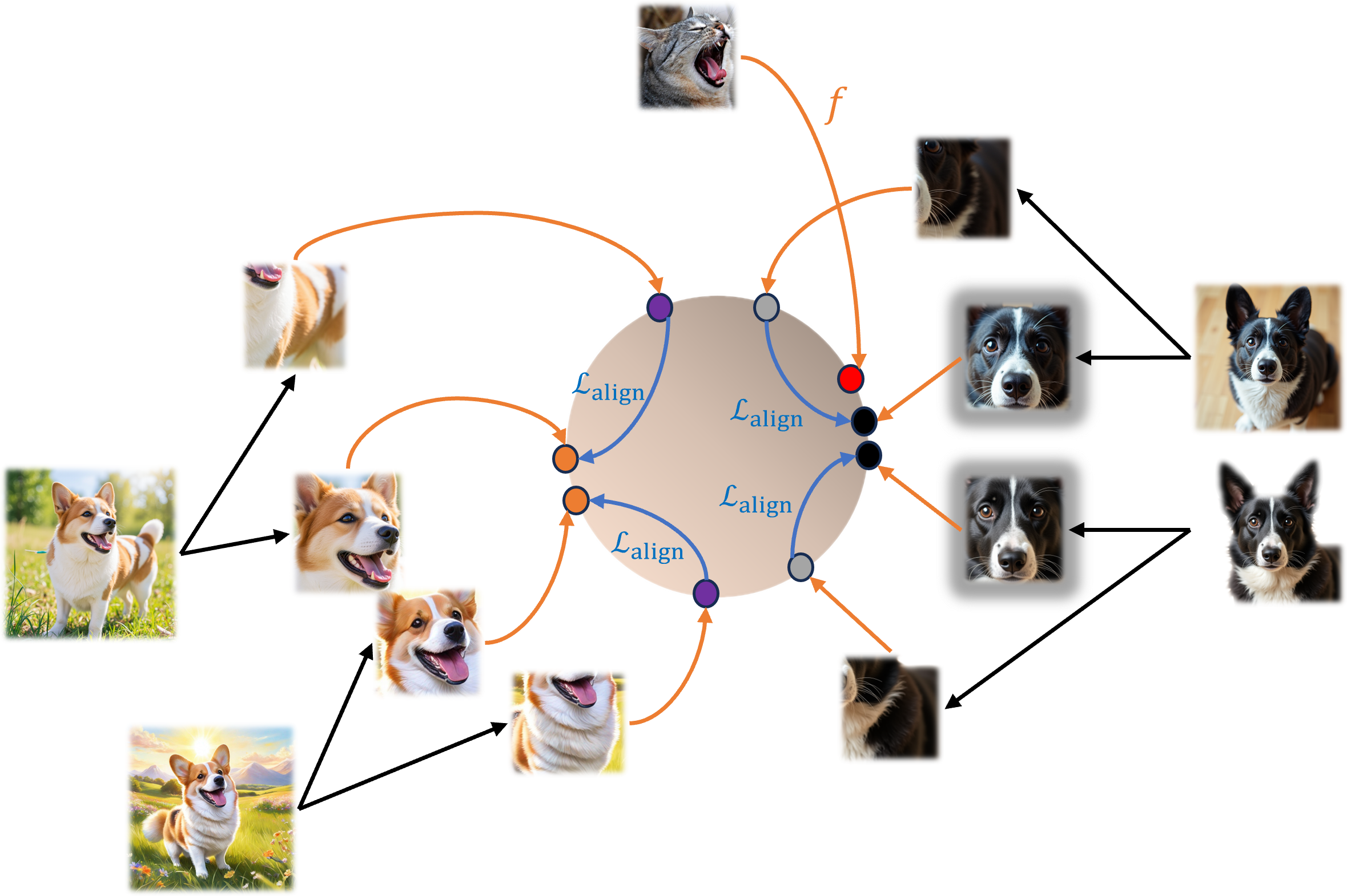
Figure 1: Data augmentation implicitly introduces weak-supervision signal.

1.1 Contributions

Our main contributions are summarized as follows:

• We introduce a novel self-supervised learning method, termed Distribution Matching (DM). DM drives the representation distribution towards a predefined reference distribution, resulting in a learned representation space with strong geometric intuition, while the hyperparameters are easily interpretable.

• The experimental results across various real-world datasets and evaluation metrics demonstrate that the performance of DM on the target classification task is competitive with existing self-supervised learning methods. The ablation study further confirms that DM effectively captures fine-grained concepts, which aligns with our intuition.

• We provide rigorous theoretical guarantees for DM, including a population theorem and an end-to-end sample theorem. The population theorem bridges the gap between the self-supervised learning task and target classification accuracy. The sample theorem demonstrates that, even with a limited number of downstream samples, DM can achieve exceptional classification performance, provided the size of the unlabeled sample set is sufficiently large.

1.2 Related works

Huang et al. (2023) establish a theoretical foundation for various self-supervised losses at the population level, while Duan et al. (2024) extend this analysis to the sample level for the adversarial loss they propose. We provide theoretical guarantees at both the population and sample levels. Wang and Isola (2020); Awasthi et al. (2022); Huang et al. (2023); Duan et al. (2024) have investigated the structure of the representation space learned by various self-supervised learning methods, both empirically and theoretically. In contrast, DM naturally exhibits a clear geometric structure. HaoChen et al. (2021, 2022); HaoChen and Ma (2023) suggest the existence of a potential subclass structure within their graph-theoretical framework, though without empirical support. By leveraging the clear geometric structure and the interpretability of DM’s hyperparameters, the ablation experiment presented in Section 4.2 empirically verifies this hypothesis.

2 Methodology

Let $\bm{x}=(x_{1},\cdots,x_{d})^{\top}\in\mathbb{R}^{d}$ be an arbitrary $d$-dimensional vector, we define $\|{\bm{x}}\|_{p}=(\sum_{i}|{x_{i}}|^{p})^{\frac{1}{p}}$ be its $p$-norm with $p\in\{1,2,\infty\}$. In particular, for $p=\infty$, $\|{\bm{x}}\|_{\infty}=\max_{i}|{x_{i}}|$. Let $f$ be a function from $\mathbb{R}^{d_{1}}$ to $\mathbb{R}^{d_{2}}$, and let $\mathrm{dom}(f)$ represent the domain of $f$. For a constant $c\geq 0$, we say that $f$ satisfies $\|{f}\|_{2}=c$ if $\|{f(\bm{x})}\|_{2}=c$ holds for any $\bm{x}\in\mathrm{dom}(f)$. Additionally, we define the functional set as:

$$\mathrm{Lip}(L)=\Big{\{}f:\mathbb{R}^{d_{1}}\to\mathbb{R}^{d_{2}}\Big{|}\sup_{\begin{subarray}{c}\bm{x}_{1},\bm{x}_{2}\in\mathrm{dom}(f)\\ \bm{x}_{1}\neq\bm{x}_{2}\end{subarray}}\frac{\|{f(\bm{x}_{1})-f(\bm{x}_{2})}\|_{2}}{\|{\bm{x}_{1}-\bm{x}_{2}}\|_{2}}\leq L\Big{\}}.$$ (1)

Let $f$ and $g$ be two functions defined on $\mathbb{N}=\{1,2,\cdots\}$. We say that $f(n)\leq\mathcal{O}(g(n))$ if and only if there exist two fixed constants $0<c_{1}\leq c_{2}$ and a positive integer $n_{0}\in\mathbb{N}$, such that for all $n\geq n_{0},c_{1}g(n)\leq f(n)\leq c_{2}g(n)$. It immediately follows that $c_{2}^{-1}f(n)\leq g(n)\leq c_{1}^{-1}f(n)$ for any $n\geq n_{0}$. Therefore, the statement $f(n)=\mathcal{O}(g(n))$ implies that $g(n)=\mathcal{O}(f(n))$. Given two quantities $X$ and $Y$, we use $X\lesssim Y$ or $Y\gtrsim X$ to denote $X\leq cY$ for some constant $c>0$.

Assume a source dataset containing a total of $n_{S}$ unlabeled image instances, denoted by $\mathcal{D}_{S}=\{X_{S}^{(i)}:1\leq i\leq n_{S}\}$, Here $X_{S}^{(i)}\in\mathcal{X}_{S}\subseteq[0,1]^{d}$ represents the $i$-th instance, which are independently and identically generated from a source distribution $\mathbb{P}_{S}$ on the source domain $\mathcal{X}_{S}$. To fix the idea, consider the ImageNet dataset as an example for $\mathcal{D}_{S}$. We then have a total of $n_{S}=1.28\times 10^{6}$ instances (Deng et al., 2009). Since ImageNet instance are of $224\times 224\times 3$ resolution, we thus have $d=150,528=224\times 224\times 3$. Next, assume a target dataset as $\mathcal{D}_{T}=\{(X_{T}^{(i)},Y_{i}):1\leq i\leq n_{T}\}$ with $X_{T}^{(i)}\in[0,1]^{d}$ and $Y_{i}\in\{1,2,\cdots,K\}$ being the class label. Assume $(X_{T}^{(i)},Y_{i})$s are independently and identically generated from a target distribution $\mathbb{P}_{T}$. For most real applications, we typically have $n_{S}\gg n_{T}$. How to leverage $\mathcal{D}_{S}$ so that a model with excellent classification accuracy on $\mathcal{D}_{T}$ is a problem of great intent.

2.1 Data Representation

Pixel images pose significant challenges for statistical learning for at least two reasons. First, their high dimensionality, as exemplified by ImageNet with 150,528 dimensions per image, complicates statistical modeling. Second, pixel images are inherently noisy. For example, consider Figure 2, where the left panel ($\bm{x}_{1}$) shows a photo of a dog, the middle panel ($\bm{x}_{2}$) shows a different image, and the right panel ($\bm{x}_{3}$) shows a cropped version of $\bm{x}_{1}$. Intuitively, $\bm{x}_{1}$ and $\bm{x}_{3}$ should be more similar, yet Euclidean distance calculations reveal $\|{\bm{x}_{1}-\bm{x}_{2}}\|_{2}<\|{\bm{x}_{1}-\bm{x}_{3}}\|_{2}$. This counterintuitive result highlights that pixel vectors encode both useful semantic information and significant noise, making the transformation to a lower-dimensional, less noisy representation crucial.

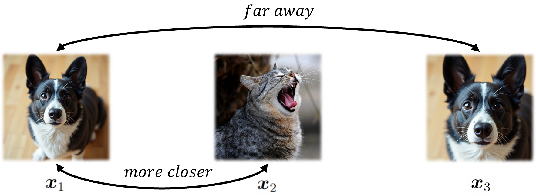
Figure 2: The semantic meaning of $\bm{x}_{1}$ and $\bm{x}_{2}$ are almost same since $\bm{x}_{3}$ is a cropped version of $\bm{x}_{1}$. However, we have $\|{\bm{x}_{1}-\bm{x}_{2}}\|_{2}<\|{\bm{x}_{1}-\bm{x}_{3}}\|_{2}$.

This leads to the concept of data representation (Rumelhart et al., 1986; Bengio et al., 2012; LeCun et al., 2015). By “data representation”, we refer to mapping an original image $X\in\mathbb{R}^{d}$ to a lower-dimensional space $f(X)\in\mathbb{R}^{d^{*}}$, where $d^{*}\ll d$. Here $f$ is typically a nonlinear function from $\mathbb{R}^{d}$ to $\mathbb{R}^{d^{*}}$. We refer to $f$ as an encoder and the range of $f$ as the representation space. A crucial question is: what defines a useful encoder? Intuitively, an effective encoder should map semantically similar images to nearby points in the representation space, while images with distinct semantic content should be well-separated. This principle has inspired many supervised representation learning methods (Hoffer and Ailon, 2015; Chopra et al., 2005; Zhai and Wu, 2018), which rely on accurately annotated labels. Instances with the same label are treated as semantically similar, while those with different labels are considered distinct.

These methods excel in preserving similarity among instances with the same label, but they have notable limitations. First, annotation is costly, particularly for large datasets (Albelwi, 2022). Second, they fail to fully capture the richness of semantic meanings. For instance, an image labeled as toilet paper in the ImageNet dataset (Figure 3) could also be labeled as bike, man, road, and others. By assigning a single label, we lose the opportunity to capture these additional semantic meanings, leading to significant information loss. Thus, developing efficient representation learning methods that minimize this loss is a key research challenge.

Figure 3: Images labeled by toilet paper in ImageNet

2.2 Self-Supervised Contrastive Learning

In the absence of labeled data, the need for effective representations has driven the development of contrastive learning. The core idea is to learn representations invariant to augmentations. By augmentation, we refer to a predefined function that transforms an image $A(\cdot)$ into a similar, but not identical image $A(X)\in\mathbb{R}^{d}$. In practice, $X$ and $A(X)$ might be of different dimensions. For notation simplicity, we assume they share the same dimension in this work. Since $A(X)$ is derived from $X$, they are expected to share similar semantic meanings. Commonly used augmentation include random cropping, flipping, translation, rescaling, color distortion, grayscale, normalization, and their compositions (see Chen et al. (2020a) and Wang et al. (2024) for details). We define the set of augmentations as $\mathcal{A}=\{A_{m}(\cdot):1\leq m\leq M\}$, where $M$ represents the total number of augmentations. While $M$ could be infinite, we consider a sufficiently large finite $M$ for theoretical convenience. With a large enough $M$, any augmentation can be well-approximated by some $A\in\mathcal{A}$. For convenience in derivation, we assume the identity transformation is included in $\mathcal{A}$.

We now introduce the concept of augmentation invariance, which means that $\|f(\mathtt{X}_{1})-f(\mathtt{X}_{2})\|_{2}^{2}$ should be minimized, where $\mathtt{X}_{1}$ and $\mathtt{X}_{2}$ are augmented from the same original image. Let $\mathcal{A}(X)=\{A(X):A\in\mathcal{A}\}$ be the set of all augmented views of $X$, and let $\mathtt{X}\sim\mathcal{A}(X)$ indicates that $\mathtt{X}$ is sample uniformly from $\mathcal{A}(X)$ according to a uniform distribution. Following (Huang et al., 2023; Duan et al., 2024), we define the alignment loss function $\mathcal{L}_{\mathrm{align}}(f)$ as:

$$\mathcal{L}_{\mathrm{align}}(f)=\mathbb{E}_{X_{S}\sim\mathbb{P}_{S}}\mathbb{E}_{\mathtt{X}_{S,1},\mathtt{X}_{S,2}\sim\mathcal{A}(X_{S})}\Big{\{}\Big{\|}f(\mathtt{X}_{S,1})-f(\mathtt{X}_{S,2})\Big{\|}_{2}^{2}\Big{\}}.$$ (2)

Furthermore, given $L>0,R>0$, we define a functional class as

$$\mathcal{F}=\big{\{}f:[0,1]^{d}\to\mathbb{R}^{d^{*}}\big{|}f\in\mathrm{Lip}(L)\text{ and }\|{f}\|_{2}=R\big{\}}.$$ (3)

Theoretically, the optimal encoder is $f_{\mathrm{opt}}\in\operatorname*{arg\,min}_{f\in\mathcal{F}}\mathcal{L}_{\mathrm{align}}(f)$. However, this results in an trivial solution where $f_{\mathrm{opt}}\equiv\bm{p}\in\mathbb{R}^{d^{*}}$, a fixed point with $\|{\bm{p}}\|_{2}=R$. which is ineffective for the learning task. This issue is referred to as model collapse (Jing et al., 2021; Zbontar et al., 2021).

To prevent model collapse, several effective techniques have been developed. The fundamental idea behind Ye et al. (2019); He et al. (2020); Chen et al. (2020a); HaoChen et al. (2021) is to identify an encoder that pushes the augmented views of different images far apart while minimizing (2). Therein, the augmented views of different images are dubbed as negative samples. Nevertheless, as noted by Chuang et al. (2020, 2022), brutally pushing far apart negative samples can hinder representation learning, as these samples may share similar or even identical semantic meaning. Consequently, efficient representation learning without negative samples has become a significant research focus. Methods like Zbontar et al. (2021); Ermolov et al. (2021); Bardes et al. (2022); HaoChen et al. (2022) propose regularization techniques on $f$ to ensure non-degenerate representation variability. A common approach  (HaoChen et al., 2022; HaoChen and Ma, 2023; Duan et al., 2024) constrains $\mathbb{E}_{X_{S}\sim\mathbb{P}_{S}}\mathbb{E}_{\mathtt{X}_{S,1},\mathtt{X}_{S,2}\sim\mathcal{A}(X_{S})}\{f(\mathtt{X}_{S,1})f(\mathtt{X}_{S,2})^{\top}\}$ to be close to the identity matrix, demonstrating effectiveness but lacking interpretability. As an alternative, we propose distribution matching (DM), which defines a reference distribution in the representation space and minimizes the Mallows’ distance to align the learned distribution with this reference, offering a clear geometric interpretation.

2.3 Distribution Matching

Before introducing the DM method, we briefly review the Mallows’ distance (Mallows, 1972; Shao and Tu, 2012), also known as the Wasserstein distance (Villani, 2009). To do so, we first define some key concepts. Let $\nu$ be a measure on $\mathbb{R}^{d_{1}}$ and $f:\mathbb{R}^{d_{1}}\rightarrow\mathbb{R}^{d_{2}}$ a measurable function. The push-forward measure $f_{\sharp}\nu$ is defined as $f_{\sharp}\nu(E)=\nu(f^{-1}(E))$ for any $f_{\sharp}\nu$-measurable set $E\subseteq\mathbb{R}^{d_{2}}$. In this context, the Mallows’ distance is defined as:

Definition 1 (Mallows’ distance).

Let $(\mathcal{X}_{1},\nu_{1})$ and $(\mathcal{X}_{2},\nu_{2})$ are two probability spaces with $\mathcal{X}_{1},\mathcal{X}_{2}\subseteq\mathbb{R}^{k}$ for some positive integer $k$. Then the Mallow’s distance is defined as

$$\mathcal{W}(\nu_{1},\nu_{2})=\inf_{(X_{1},X_{2})\in\Pi(\nu_{1},\nu_{2})}\mathbb{E}_{(X_{1},X_{2})}\Big{(}\|{X_{1}-X_{2}}\|_{1}\Big{)},$$ (4)

where $\Pi(\nu_{1},\nu_{2})$ denotes the collection of all possible joint distributions of the pairs $(X_{1},X_{2})$ with marginal distributions given by $\nu_{1}$ and $\nu_{2}$, respectively. Here we implicitly assume that there exists a probability space $(\Omega,P)$ such that $X_{1}:\Omega\to\mathcal{X}_{1}$ and $X_{2}:\Omega\to\mathcal{X}_{2}$ are measurable and satisfy $(X_{1})_{\sharp}P=\nu_{1}$ and $(X_{2})_{\sharp}P=\nu_{2}$.

To better understand the Definition 1, we explore a special case in detail. Let $\mathcal{X}_{1}=\{\bm{x}_{1,1},\bm{x}_{1,2},\cdots,\bm{x}_{1,n_{1}}\}\subseteq\mathbb{R}^{k}$ and $\mathcal{X}_{2}=\{\bm{x}_{2,1},\bm{x}_{2,2},\cdots,\bm{x}_{2,n_{2}}\}\subseteq\mathbb{R}^{k}$, where $k,n_{1}$ and $n_{2}$ are positive integers. Suppose $\nu_{1}$ and $\nu_{2}$ are discrete probability distributions on $\mathcal{X}_{1}$ and $\mathcal{X}_{2}$, respectively. Then each element in $\Pi(\nu_{1},\nu_{2})$ can be completely determined by a discrete probability distribution on the cartesian product $\mathcal{X}_{1}\times\mathcal{X}_{2}$, represented by $\Psi(\bm{x}_{1},\bm{x}_{2})\in\mathbb{R}^{n_{1}\times n_{2}}$. Accordingly, it should satisfy that (i) $\Psi(\bm{x}_{1},\bm{x}_{2})\geq 0$ for any $\bm{x}_{1}\in\mathcal{X}_{1}$ and $\bm{x}_{2}\in\mathcal{X}_{2}$, (ii) $\sum_{\bm{x}_{1},\bm{x}_{2}}\Psi(\bm{x}_{1},\bm{x}_{2})=1$, (iii) $\sum_{\bm{x}_{2}\in\mathcal{X}_{2}}\Psi(\bm{x}_{1},\bm{x}_{2})=\nu_{1}(\bm{x}_{1})$ for any $\bm{x}_{1}\in\mathcal{X}_{1}$ and (iv) $\sum_{\bm{x}_{1}\in\mathcal{X}_{1}}\Psi(\bm{x}_{1},\bm{x}_{2})=\nu_{2}(\bm{x}_{2})$ for any $\bm{x}_{2}\in\mathcal{X}_{2}$. The Mallows’ distance between $\nu_{1}$ and $\nu_{2}$ is then given by: $\mathcal{W}(\nu_{1},\nu_{2})=\inf_{\Psi\in\Pi(\nu_{1},\nu_{2})}\sum_{\bm{x}_{1}\in\mathcal{X}_{1},\bm{x}_{2}\in\mathcal{X}_{2}}\Psi(\bm{x}_{1},\bm{x}_{2})\cdot\|{\bm{x}_{1}-\bm{x}_{2}}\|_{1}$. Intuitively, $\nu_{1}$ and $\nu_{2}$ can be regarded as two piles of probability masses, with $\nu_{1}(\bm{x}_{1})$ and $\nu_{2}(\bm{x}_{2})$ indicating the mass at $\bm{x}_{1}$ and $\bm{x}_{2}$, respectively. The transport plan $\Psi(\bm{x}_{1},\bm{x}_{2})$ can be thought of as the amount of mass transported from $\bm{x}_{1}$ and $\bm{x}_{2}$, while the term $\|{\bm{x}_{1}-\bm{x}_{2}}\|_{1}$ represents the transportation cost. Thus, the Mallows’ distance quantifies the minimal cost to transport one probability distribution to another.

Although Definition 1 is intuitive, computing it is challenging due to the difficulty of finding the optimal coupling in $\Pi(\nu_{1},\nu_{2})$. To address this, a dual formulation is provided in Remark 6.5 of Villani (2009):

$$\mathcal{W}(\nu_{1},\nu_{2})=\sup_{g\in\mathrm{Lip}(1)}\mathbb{E}_{X_{1}\sim\nu_{1}}\Big{\{}g(X_{1})\Big{\}}-\mathbb{E}_{X_{2}\sim\nu_{2}}\Big{\{}g(X_{2})\Big{\}},$$ (5)

where the task reduces to finding the optimal function $g$ in $\mathrm{Lip}(1)$, , a problem that can be solved using a neural network with gradient penalty (Gulrajani et al., 2017), as detailed in (19). Notably, the Mallows’ distance remains effective even when $\nu_{1}$ and $\nu_{2}$ have different supports, unlike many other divergence measures (e.g., Kullback-Leibler and Jensen-Shannon divergence), which either diverge to infinite or become constant in such cases. Furthermore, the Mallows’ distance satisfies the triangle inequality, making it a true distance metric, an important property not shared by many other divergence measures. For a thorough theoretical treatment of Mallows’ distance, we refer to Villani (2009).

With the Mallows’ distance defined, we can now proceed to develop the DM method. The key idea is to prevent model collapse by minimizing the Mallows’ distance between the representation distribution and the predefined reference distribution. As a result, constructing the reference distribution becomes the most crucial step, which can be broken down into three sub-steps. In the first sub-step, we design $K^{\prime}$ centers in $\mathbb{R}^{d^{*}}$ , where $K^{\prime}\leq d^{*}$. The $i$-th center $\bm{c}_{i}$ is chosen to be either $\bm{e}_{i}$ or $-\bm{e}_{i}$ with equal probability, where $\bm{e}_{i}$ is the standard basis vector in $\mathbb{R}^{d^{*}}$ with the $i$-th component equal to $1$ and all others components equal to $0$. In the second sub-step, we define the $i$-th reference part a random vector as:

$$\mathcal{P}_{i}=R\frac{\bm{c}_{i}+\epsilon\frac{\bm{\gamma}_{d^{*}}}{\|{\bm{\gamma}_{d^{*}}}\|_{2}}}{\big{\|}\bm{c}_{i}+\epsilon\frac{\bm{\gamma}_{d^{*}}}{\|{\bm{\gamma}_{d^{*}}}\|_{2}}\big{\|}_{2}},$$ (6)

where $\epsilon>0$ is a tuning parameter, and $\bm{\gamma}_{d^{*}}$ is a standard Gaussian random vector in $\mathbb{R}^{d^{*}}$. To gain an intuitive understanding of $\mathcal{P}_{i}$, let $\mathcal{B}(\bm{a},r)$ denote the ball centered at $\bm{a}\in\mathbb{R}^{d^{*}}$ with radius $r>0$. It is straightforward to observe that the vector $\bm{\gamma}_{d^{*}}/\|{\bm{\gamma}_{d^{*}}}\|_{2}$ follows a uniform distribution on the surface of the unit ball $\mathcal{B}(\bm{0},1)$. We then scale and translate this vector to lie within the ball $\mathcal{B}(\bm{c}_{i},\epsilon)$ by multiplying by $\epsilon$ and adding the center $\bm{c}_{i}$. To ensure that the resulting random variable $\mathcal{P}_{i}$ lies on the surface of the ball $\mathcal{B}(\bm{0},R)$, we normalize the vector and scale it by $R$. As shown in the left-hand side of Figure 4, the process results in $\mathcal{P}_{i}$ follows a uniform distribution over the orange region of the sphere. Next, we define a categorical random variable $\mathcal{C}\in\{1,2,\cdots,K^{\prime}\}$ with $\mathbb{P}(\mathcal{C}=i)=\alpha_{i}$, where $\alpha_{i}$ are the probabilities associated with $i$-th part, and $\mathcal{C}$ is independent of $\mathcal{P}_{i}$ for all $1\leq i\leq K^{\prime}$. We then construct a new random variable $\mathcal{R}$ as $\mathcal{R}=\sum_{i=1}^{K^{\prime}}\mathbbm{1}(\mathcal{C}=i)\mathcal{P}_{i}$. The distribution of $\mathcal{R}$ is referred to as the reference distribution, denoted by $\mathbb{P}_{\mathcal{R}}$. DM aim to cluster augmented views with similar semantic meaning according to the same part of the reference distribution by minimizing $\mathcal{W}(\mathbb{P}_{f},\mathbb{P}_{\mathcal{R}})$, as illustrated on the right hand side of Figure 4.

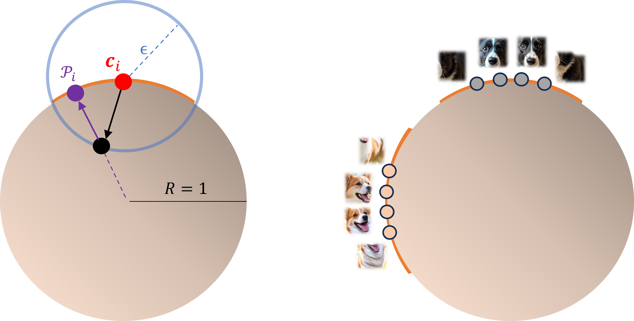
Figure 4: Left. Generative process of $\mathcal{P}_{i}$ ($R=1$). Given $\bm{c}_{i}$ (red point) and $\epsilon$, the black point is obtained by adding $\bm{c}_{i}$ and $\epsilon\bm{\gamma}_{d^{*}}/\|{\bm{\gamma}_{d^{*}}}\|_{2}$. Normalizing this into the sphere of radius $R$ yields a sample of $\mathcal{P}_{i}$ (purple point). This process results in $\mathcal{P}_{i}$ following a uniform distribution on the orange region of the sphere. Right: The key idea of DM. Augmented views with similar semantic meaning are mapped to the same region of the reference distribution.

We define the representation distribution $\mathbb{P}_{f}=f_{\sharp}\mathbb{P}_{\mathcal{A}}$, where $\mathbb{P}_{\mathcal{A}}$ is the distribution of augmented views. This is rigorously given by $\mathbb{P}_{\mathcal{A}}(E)=\int\frac{1}{M}\sum_{A\in\mathcal{A}}\mathbbm{1}\{A(\bm{x})\in E\}\mathbb{P}_{S}(d\bm{x})$ for any measurable set $E$. The DM learning problem is then formulated as the following minimization problem:

$$f^{*}\in\operatorname*{arg\,min}_{f\in\mathcal{F}}\mathcal{L}(f):=\mathcal{L}_{\mathrm{align}}(f)+\lambda\cdot\mathcal{W}(\mathbb{P}_{f},\mathbb{P}_{\mathcal{R}}).$$ (7)

where $\mathcal{L}(f)$ is the objective function that consists of alignment loss and the Wasserstein distance between $\mathbb{P}_{f}$ and $\mathbb{P}_{\mathcal{R}}$. The tuning parameter $\lambda>0$ balances the relative importance of $\mathcal{L}_{\mathrm{align}}(f)$ and $\mathcal{W}(\mathbb{P}_{f},\mathbb{P}_{\mathcal{R}})$. The function class $\mathcal{F}$ is defined in (3). It is important to note that the solution $f^{*}$ to this minimization problem may bot be unique, as $f\in\min_{f\in\mathcal{F}}\mathcal{L}(f)$ implies multiple possible minimizer. Let $\mathcal{G}:=\mathrm{Lip(1)}$ and plug (2) and (5) into (7) gives the following formulation of the DM learning problem:

$$f^{*}\in\operatorname*{arg\,min}_{f\in\mathcal{F}}\mathop{\mathbb{E}}_{X_{S}\sim\mathbb{P}_{S}}\mathop{\mathbb{E}}_{\mathtt{X}_{S,1},\mathtt{X}_{S,2}\sim\mathcal{A}(X_{S})}\Big{\|}f(\mathtt{X}_{S,1})-f(\mathtt{X}_{S,2})\Big{\|}_{2}^{2}+\lambda\sup_{g\in\mathcal{G}}\mathop{\mathbb{E}}_{Z\sim\mathbb{P}_{f}}g(Z)-\mathop{\mathbb{E}}_{\mathcal{R}\sim\mathbb{P}_{\mathcal{R}}}g(\mathcal{R}).$$ (8)

It is evident that (8) can be interpreted as a mini-max optimization problem. To emphasize this, we rewrite it as follows:

$$(f^{*},g^{*})\in\arg\min_{f\in\mathcal{F}}\max_{g\in\mathcal{G}}\mathcal{L}(f,g):=\mathcal{L}_{\mathrm{align}}(f)+\lambda\cdot\mathcal{W}(f,g),$$ (9)

where $\mathcal{W}(f,g)=\mathop{\mathbb{E}}_{Z\sim\mathbb{P}_{f}}\{g(Z)\}-\mathop{\mathbb{E}}_{\mathcal{R}\sim\mathbb{P}_{\mathcal{R}}}\{g(\mathcal{R})\}$, $g$ is referred to as a critic. It immediately follows that $\mathcal{W}(\mathbb{P}_{f},\mathbb{P}_{\mathcal{R}})=\sup_{g\in\mathcal{G}}\mathcal{W}(f,g)$ and $\mathcal{L}(f)=\sup_{g\in\mathcal{G}}\mathcal{L}(f,g)$.

To solve (9) in practice, we face two challenges. The first challenge is the population distribution of the original images $\mathbb{P}_{S}$ is unknown. We therefore have to replace it by its finite sample counterpart. Specifically, for each instance $X_{S}^{(i)}$, we sample two augmentations $A_{i,1}$ and $A_{i,2}$ from $\mathcal{A}$ uniformly. These augmentations produce two views, $\tilde{\mathtt{X}}_{S}^{(i)}=(\mathtt{X}^{(i)}_{S,1},\mathtt{X}^{(i)}_{S,2})=(A_{i,1}(X_{S}^{(i)}),A_{i,2}(X_{S}^{(i)}))\in\mathbb{R}^{2d}$. Simultaneously, we independently collect $n_{S}$ instances $\{\mathcal{R}^{(i)}:1\leq i\leq n_{S}\}$ from $\mathbb{P}_{\mathcal{R}}$. The resulting augmentation-reference dataset is $\widetilde{\mathcal{D}}_{S}=\{(\tilde{\mathtt{X}}_{S}^{(i)},\mathcal{R}^{(i)}):1\leq i\leq n_{S}\}$. The finite sample approximation of $\mathcal{L}(f,g)$ is then:

$$\widehat{\mathcal{L}}(f,g):=\widehat{\mathcal{L}}_{\mathrm{align}}(f)+\lambda\cdot\widehat{\mathcal{W}}(f,g),$$

$$\widehat{\mathcal{L}}_{\mathrm{align}}(f)=\frac{1}{n_{S}}\sum_{i=1}^{n_{S}}\|{f(\mathtt{X}^{(i)}_{S,1})-f(\mathtt{X}^{(i)}_{S,2})}\|_{2}^{2},$$

$$\widehat{\mathcal{W}}(f,g)=\frac{1}{n_{S}}\sum_{i=1}^{n_{S}}\Big{[}g(\mathcal{R}^{(i)})-\frac{1}{2}\Big{\{}g\big{(}f(\mathtt{X}^{(i)}_{S,1})\big{)}+g\big{(}f(\mathtt{X}^{(i)}_{S,2})\big{)}\Big{\}}\Big{]}.$$ (10)

It is evident that $\mathcal{W}(f,g)=\mathbb{E}_{\widetilde{\mathcal{D}}_{S}}\{\widehat{\mathcal{W}}(f,g)\}$ and $\mathcal{L}(f,g)=\mathbb{E}_{\widetilde{\mathcal{D}}_{S}}\{\widehat{\mathcal{L}}(f,g)\}$, which justifies calling $\widehat{\mathcal{L}}(f,g)$ the finite sample counterpart of $\mathcal{L}(f,g)$.

The second challenge stems from the complexity of the functional spaces $\mathcal{F}$ and $\mathcal{G}$, which complicates practical search. To overcome this, we parametrize them using deep ReLU networks. Specifically, we define a class of deep ReLU networks as follows:

Definition 2 (Deep ReLU network class).

The function $f_{\bm{\theta}}(\bm{x}):\mathbb{R}^{p}\to\mathbb{R}^{q}$ implemented by a deep ReLU network with parameter $\bm{\theta}$ is expressed as composition of a sequence of functions

$$f_{\bm{\theta}}(\bm{x}):=l_{\mathtt{D}}\circ\varrho\circ l_{\mathtt{D}-1}\circ\varrho\circ\cdots\circ l_{1}\circ\varrho\circ l_{0}(\bm{x})$$

for any $\bm{x}\in\mathbb{R}^{p}$, where $\varrho(\bm{x})$ is the ReLU activation function and the depth $\mathtt{D}$ is the number of hidden layers. For $1\leq i\leq\mathtt{D}$, the $i$-th layer is represented by $l_{i}(\bm{x}):=A_{i}\bm{x}+\bm{b}_{i}$, where $A_{i}\in\mathbb{R}^{d_{i+1}\times d_{i}}$ is the weight matrix, $\bm{b}_{i}\in\mathbb{R}^{d_{i+1}}$ is the bias vector, $d_{i}$ is the width of the $i$-th layer and $\bm{\theta}=((A_{0},\bm{b}_{0}),\cdots,(A_{\mathtt{D}},\bm{b}_{\mathtt{D}}))$. The network $f_{\bm{\theta}}$ contains $(\mathtt{D}+1)$ layers in all. We use a $(\mathtt{D}+1)$-dimension vector $(d_{0},d_{1},\cdots,d_{\mathtt{D}})^{\top}$ to describe the width of each layer. In particular, $d_{0}=p$ is the dimension of the domain and $d_{\mathtt{D}}=q$ is the dimension of the codomain. The width $\mathtt{W}$ is defined as the maximum width of hidden layers, that is, $\mathtt{W}=\max\left\{d_{1},d_{2},\cdots,d_{\mathtt{D}}\right\}$. The bound $\mathtt{B}$ denotes the $L^{\infty}$ bound of $f_{\bm{\theta}}(\cdot)$, that is, $\sup_{\bm{x}\in\mathbb{R}^{p}}\|f_{\bm{\theta}}(\bm{x})\|_{\infty}\leq\mathtt{B}$. We denote the function class $\{f_{\bm{\theta}}:\mathbb{R}^{p}\to\mathbb{R}^{q}\}$ implemented by deep ReLU network class with width $\mathtt{W}$, depth $\mathtt{D}$, and bound $\mathtt{B}$ as $\mathcal{NN}_{p,q}(\mathtt{W},\mathtt{D},\mathtt{B})$.

By parametrizing $\mathcal{F}$ and $\mathcal{G}$ as two deep ReLU network classes, the optimization problem in (9) is reformulated as:

$$(\hat{f}_{n_{S}},\hat{g}_{n_{S}})\in\arg\min_{f\in\widehat{\mathcal{F}}}\max_{g\in\widehat{\mathcal{G}}}\widehat{\mathcal{L}}(f,g),$$ (11)

where $\widehat{\mathcal{F}}=\mathcal{NN}_{d,d^{*}}(\mathtt{W}_{1},\mathtt{D}_{1},\mathtt{B}_{1})$ and $\widehat{\mathcal{G}}=\mathcal{NN}_{d^{*},1}(\mathtt{W}_{2},\mathtt{D}_{2},\mathtt{B}_{2})$. In practice, we set $\mathtt{W}_{1}\gtrsim\mathtt{W}_{2}$ and $\mathtt{D}_{1}\gtrsim\mathtt{D}_{2}$, ensuring that $\mathtt{W}_{1}\mathtt{D}_{1}\gtrsim\mathtt{W}_{2}\mathtt{D}_{2}$ in subsequent analysis.

2.4 Transfer Learning

One significant application of learned representations is transfer learning. Recall $\mathcal{D}_{T}=\{(X_{T}^{(i)},Y_{i}):1\leq i\leq n_{T}\}$ denotes the target dataset. For each $X_{T}^{(i)}\in\mathcal{D}_{T}$, we sample two augmentations $A_{i,1},A_{i,2}$ from $\mathcal{A}$ uniformly, resulting in $\tilde{\mathtt{X}}_{T}^{(i)}=(\mathtt{X}_{T,1}^{(i)},\mathtt{X}_{T,2}^{(i)})=(A_{i,1}(X_{T}^{(i)}),A_{i,2}(X_{T}^{(i)}))$. The augmented dataset is then $\widetilde{\mathcal{D}}_{T}=\{(\tilde{\mathtt{X}}_{T}^{(i)},Y_{i}):1\leq i\leq n_{T}\}$. We next consider a linear classifier

$$G_{f}(\bm{x})=\mathop{\arg\max}_{1\leq k\leq K}\big{(}\widehat{W}f(\bm{x})\big{)}_{k},$$ (12)

where $(\cdot)_{k}$ denotes the $k$-th entry of the vector, and $\widehat{W}$ is a $K\times d^{*}$ matrix with its $k$-th row given by

$$\widehat{\mu}_{T}(k)=\frac{1}{2n_{T}(k)}\sum_{i=1}^{n_{T}}\{f(\mathtt{X}_{T,1}^{(i)})+f(\mathtt{X}_{T,2}^{(i)})\}\mathbbm{1}\{Y_{i}=k\},$$ (13)

where $n_{T}(k)=\sum_{i=1}^{n_{T}}\mathbbm{1}\{Y_{i}=k\}$ represents the sample size of the $k$-th class. It is evident that $\widehat{\mu}_{T}(k)$ serves as an unbiased estimator of $\mu_{T}(k)=\mathbb{E}_{(X_{T},Y)\sim\mathbb{P}_{T}}\mathbb{E}_{\mathtt{X}_{T}\sim\mathcal{A}(X_{T})}\{f(\mathtt{X}_{T})|Y=k\}$, which denotes the center of the $k$-th class in the representation space. To evaluate its performance, we examine its misclassification rate by

$$\mathrm{Err}\big{(}G_{f}\big{)}=\mathbb{P}_{T}\big{\{}G_{f}(X_{T})\neq Y\big{\}},$$

where $(X_{T},Y)$ represents an independent copy of $(X_{T}^{(i)},Y_{i})$.

3 Theoretical Guarantee

3.1 Population Theorem

We assume that any upstream data $X_{S}\sim\mathbb{P}_{S}$ can be categorized into categorized into some of $K$ latent classes, each corresponding to a distinct downstream class. The term “latent” implies that these classes are not directly observable to us, but do exist. For $1\leq k\leq K$, we define $C_{S}(k)$ as the set of data points belonging to the $k$-th latent class. The conditional probability distribution $\mathbb{P}_{f}(k)$ is given by $\mathbb{P}_{f}(k)(\cdot)=\mathbb{P}_{f}\{\cdot|X_{S}\in C_{S}(k)\}$, with its population center $\mu_{S}(k)=\mathbb{E}_{X_{S}\sim\mathbb{P}_{S}}\mathbb{E}_{\mathtt{X}_{S}\sim\mathcal{A}(X_{S})}\{f(\mathtt{X_{S}})|X_{S}\in C_{S}(k)\}$.

The goal of DM is to render source data well-separated. Specifically, we aim to drive $\mu_{S}(i)^{\top}\mu_{S}(j)$ as close to zero as possible for any $i\neq j$. To accomplish this, we aim to push $\mathbb{P}_{f}(k)$ towards distinct parts of the reference distribution through Mallows’ distance (which we refer to as “pushing $\mathbb{P}_{f}$ in parts”), thereby inheriting the characteristics of $\mathbb{P}_{\mathcal{R}}$. However, since $\mathbb{P}_{f}(k)$ is inaccessible, we must instead minimize the overall Mallows’ distance $\mathcal{W}(\mathbb{P}_{f},\mathbb{P}_{\mathcal{R}})$, and explore its effect on achieving the objective of separating the classes.

We begin by assigning labels to each part of the reference distribution. Let the predefined reference consist of $K$ disjoint parts $\{C_{k}:1\leq k\leq K\}$. Let $\mathbb{Q}^{*}$ represent the joint distribution of $(Z^{*},\mathcal{R}^{*})$, where $(Z^{*},\mathcal{R}^{*})=\arg\min_{(Z,\mathcal{R})\in\Pi(\mathbb{P}_{f},\mathbb{P}_{\mathcal{R}})}\mathbb{E}_{(Z,\mathcal{R})}(\|{Z-\mathcal{R}}\|_{1})$. Denote the set of permutations on $\{1,2,\cdots,K\}$ by $P_{K}$. The $k$-th class of the reference, $C_{\mathcal{R}}(k)$, corresponding to the $k$-th latent class $C_{S}(k)$, is defined as $C_{\mathcal{R}}(k):=C_{\tau^{*}(k)}$, where $\tau^{*}=\operatorname*{arg\,max}_{\tau\in P_{K}}\sum_{k=1}^{K}\mathbb{Q}^{*}(C_{S}(k)\to C_{\tau(k)})$. Therein, $\mathbb{Q}^{*}(C_{S}(k)\to C_{\tau(k)})$ represents the transport mass from $C_{S}(k)$ to $C_{\tau(k)}$ according to $\mathbb{Q}^{*}$. To better understand this assignment, consider an example with $K=3$ and $\mathbb{Q}^{*}$ such that $\mathbb{Q}^{*}(C_{S}(1)\to C_{1})=1/5,\mathbb{Q}^{*}(C_{S}(1)\to C_{2})=0,\mathbb{Q}^{*}(C_{S}(1)\to C_{3})=2/15;\mathbb{Q}^{*}(C_{S}(2)\to C_{1})=1/15,\mathbb{Q}^{*}(C_{S}(2)\to C_{2})=1/30,\mathbb{Q}^{*}(C_{S}(2)\to C_{3})=7/30$ and $\mathbb{Q}^{*}(C_{S}(3)\to C_{1})=4/15,\mathbb{Q}^{*}(C_{S}(3)\to C_{2})=1/30,\mathbb{Q}^{*}(C_{S}(3)\to C_{3})=1/30$. In this context, we for example evaluate two permutations: $\tau_{1}:(1,2,3)\mapsto(3,2,1)$ and $\tau_{2}:(1,2,3)\mapsto(2,3,1)$. For the permutation $\tau_{1}$, we have $\sum_{k=1}^{3}\mathbb{Q}^{*}(C_{S}(k)\to C_{\tau_{1}(k)})=\mathbb{Q}^{*}(C_{S}(1)\to C_{3})+\mathbb{Q}^{*}(C_{S}(2)\to C_{2})+\mathbb{Q}^{*}(C_{S}(3)\to C_{1})=2/15+1/30+4/15=13/30$, while $\sum_{k=1}^{3}\mathbb{Q}^{*}(C_{S}(k)\to C_{\tau_{2}(k)})=\mathbb{Q}^{*}(C_{S}(1)\to C_{2})+\mathbb{Q}^{*}(C_{S}(2)\to C_{3})+\mathbb{Q}^{*}(C_{S}(3)\to C_{1})=0+7/30+4/15=1/2$. After comparisons across all permutations, we obtain $C_{\mathcal{R}}(1)=C_{2},C_{\mathcal{R}}(2)=C_{3},C_{\mathcal{R}}(3)=C_{1}$. In summary, for given $C_{i}$, we tend to assign the label $\arg\max_{k}\mathbb{Q}^{*}(C_{S}(k)\to C_{i})$. However, it may lead to non-unique assignments. We resolve this by introducing optimal permutation.

Let $Z\in C_{S}(i)$ denote the event $Z=f(A(X_{S}))$ for some $X_{S}\in C_{S}(i)$ and $A\in\mathcal{A}$, $\mathbb{P}_{\mathcal{R}}(j)$ be the uniform distribution on $C_{\mathcal{R}}(j)$. We can yield

$$\mathcal{W}(\mathbb{P}_{f},\mathbb{P}_{\mathcal{R}}) =\int_{(Z,\mathcal{R})}\|{Z-\mathcal{R}}\|_{1}d\mathbb{Q}^{*}(Z,\mathcal{R})$$

$$=\sum_{i,j=1}^{K}\Big{\{}\int_{(Z,\mathcal{R})}\|{Z-\mathcal{R}}\|_{1}d\mathbb{Q}^{*}\big{(}Z,\mathcal{R}|Z\in C_{S}(i),\mathcal{R}\in\mathbb{P}_{\mathcal{R}}(j)\big{)}\Big{\}}\mathbb{Q}^{*}\big{(}C_{S}(i)\to\mathbb{P}_{\mathcal{R}}(j)\big{)}$$

$$\geq\sum_{i,j=1}^{K}\mathcal{W}\big{(}\mathbb{P}_{f}(i),\mathbb{P}_{\mathcal{R}}(j)\big{)}\mathbb{Q}^{*}\big{(}C_{S}(i)\to C_{\mathcal{R}}(j)\big{)}$$

$$\geq\mathbb{Q}^{*}\big{(}C_{S}(k)\to C_{\mathcal{R}}(k)\big{)}\mathcal{W}\big{(}\mathbb{P}_{f}(k),\mathbb{P}_{\mathcal{R}}(k)\big{)},$$ (14)

where the first inequality follows from $\mathbb{Q}^{*}(Z,\mathcal{R}|Z\in C_{S}(i),\mathcal{R}\in\mathbb{P}_{\mathcal{R}}(j))\in\Pi(\mathbb{P}_{f}(i),\mathbb{P}_{\mathcal{R}}(j))$. Therefore, under Assumption 1, we know that $\mathcal{W}(\mathbb{P}_{f}(k),\mathbb{P}_{\mathcal{R}}(k))\lesssim\mathcal{W}(\mathbb{P}_{f},\mathbb{P}_{\mathcal{R}})\leq\mathcal{L}(f)$.

Assumption 1.

Assume $\mathbb{Q}^{*}\big{(}C_{S}(k)\to C_{\mathcal{R}}(k)\big{)}>0$ for any $k:1\leq k\leq K$.

Assumption 1 essentially indicates that, in contrast to the example above regarding label assignments, we do not desire $C_{2}$ to be labeled as $C_{\mathcal{R}}(1)$ while $\mathbb{Q}^{*}(C_{S}(1)\to C_{2})=0$.

Furthermore, by utilizing $\bm{c}_{i}^{\top}\bm{c}_{j}=0$ and $\|{\bm{c}_{i}}\|_{2}=R$, we yield

$$\mu_{S}(i)^{\top}\mu_{S}(j) =(\mu_{S}(i)-\bm{c}_{i})^{\top}\mu_{S}(j)+\bm{c}_{i}^{\top}\mu_{S}(j)+\bm{c}_{i}^{\top}\bm{c}_{j}+\bm{c}_{i}^{\top}(\mu_{S}(j)-\bm{c}_{j})$$

$$\leq\|\mu_{S}(i)-\bm{c}_{i}\|_{2}\|\mu_{S}(j)\|_{2}+\|\bm{c}_{i}\|_{2}\|\mu_{S}(j)-\bm{c}_{j}\|_{2}$$

$$\lesssim\|\mu_{S}(i)-\bm{c}_{i}\|_{2}+\|\mu_{S}(j)-\bm{c}_{j}\|_{2},$$ (15)

where the last inequality stems from $\|{\mu_{S}(j)}\|_{2}=\big{\|}\mathbb{E}_{X_{S}\sim\mathbb{P}_{S}}\mathbb{E}_{\mathtt{X}_{S}\sim\mathcal{A}(X_{S})}\{f(\mathtt{X}_{S})|X_{S}\in C_{S}(j)\}\big{\|}_{2}\leq\mathbb{E}_{X_{S}\sim\mathbb{P}_{S}}\mathbb{E}_{\mathtt{X}_{S}\sim\mathcal{A}(X_{S})}\{\|{f(\mathtt{X}_{S})}\|_{2}\big{|}X_{S}\in C_{S}(j)\}=R$. Moreover, regarding $\|{\mu_{S}(k)-\bm{c}_{k}}\|_{2}$,

$$\|{\mu_{S}(k)-\bm{c}_{k}}\|^{2}_{2} =\sum_{l=1}^{d^{*}}\Big{[}\mathop{\mathbb{E}}_{X_{S}\in C_{S}(k)}\mathop{\mathbb{E}}_{\mathtt{X}_{S}\in\mathcal{A}(X_{S})}\big{\{}f_{l}(\mathtt{X_{S}})\big{\}}-\mathop{\mathbb{E}}_{\mathcal{R}_{k}\in C_{\mathcal{R}}(k)}\big{\{}\mathcal{R}_{k,l}\big{\}}\Big{]}^{2}$$

$$\leq\sum_{l=1}^{d^{*}}\mathcal{W}^{2}\big{(}\mathbb{P}_{f}(k),\mathbb{P}_{\mathcal{R}}(k)\big{)}=d^{*}\mathcal{W}^{2}\big{(}\mathbb{P}_{f}(k),\mathbb{P}_{\mathcal{R}}(k)\big{)}$$

$$\lesssim\mathcal{W}^{2}\big{(}\mathbb{P}_{f}(k),\mathbb{P}_{\mathcal{R}}(k)\big{)},$$ (16)

where the first inequality follows from (5). Plugging (3.1) into (3.1) yields $\mu_{S}(i)^{\top}\mu_{S}(j)\lesssim\mathcal{L}(f)$, implying that minimizing the loss function of DM can indeed reduce $\mu_{S}(i)^{\top}\mu_{S}(j)$.

We now show that minimizing $\mathcal{L}(f)$ also reduces $\mu_{T}(i)^{\top}\mu_{T}(j)$. It suffices to explore the relationship between $\mu_{S}(i)^{\top}\mu_{S}(j)$ and $\mu_{T}(i)^{\top}\mu_{T}(j)$. Let $\mathbb{P}_{T}(k)$ be the distribution defined by $\mathbb{P}_{T}(k)(E)=\mathbb{P}_{T}(X_{S}\in E|Y=k)$ for any measurable set $E$, with $p_{S}(k)=\mathbb{P}_{S}\{X_{S}\in C_{S}(k)\}$ and $p_{T}(k)=\mathbb{P}_{T}(Y=k)$. To quantify the distribution shift, we define

$$\epsilon_{1}=\max_{k}\mathcal{W}\big{(}\mathbb{P}_{S}(k),\mathbb{P}_{T}(k)\big{)},\quad\epsilon_{2}=\max_{k}|{p_{S}(k)-p_{T}(k)}|.$$ (17)

Thus, we have

$$\mu_{T}(i)^{\top}\mu_{T}(j)-\mu_{S}(i)^{\top}\mu_{S}(j) =\mu_{T}(i)^{\top}\mu_{T}(j)-\mu_{T}(i)^{\top}\mu_{S}(j)+\mu_{T}(i)^{\top}\mu_{S}(j)-\mu_{S}(i)^{\top}\mu_{S}(j)$$

$$=\mu_{T}(i)^{\top}\{\mu_{T}(j)-\mu_{S}(j)\}+\{\mu_{T}(i)-\mu_{S}(i)\}^{\top}\mu_{S}(j)$$

$$\leq\|{\mu_{T}(i)}\|_{2}\|{\mu_{T}(j)-\mu_{S}(j)}\|_{2}+\|{\mu_{T}(i)-\mu_{S}(i)}\|_{2}\|{\mu_{S}(j)}\|_{2}$$

$$\leq R\big{\{}\|{\mu_{T}(j)-\mu_{S}(j)}\|_{2}+\|{\mu_{T}(i)-\mu_{S}(i)}\|_{2}\big{\}}.$$

Moreover, for any $1\leq k\leq K$, we have:

$$\|{\mu_{S}(k)-\mu_{T}(k)}\|_{2}^{2}=\sum_{l=1}^{d^{*}}\Big{[}\big{\{}\mu_{S}(k)\big{\}}_{l}-\big{\{}\mu_{T}(k)\big{\}}_{l}\Big{]}^{2}$$

$$=\sum_{l=1}^{d^{*}}\Big{[}\mathbb{E}_{X_{S}\sim\mathbb{P}_{S}}\mathbb{E}_{\mathtt{X}_{S}\sim\mathcal{A}(X_{S})}\big{\{}f_{l}(\mathtt{X}_{S})|X_{S}\in C_{S}(k)\big{\}}-\mathbb{E}_{(X_{T},Y)\sim\mathbb{P}_{T}}\mathbb{E}_{\mathtt{X}^{T}\sim\mathcal{A}(X_{T})}\big{\{}f_{l}(\mathtt{X}^{T})|Y=k\big{\}}\Big{]}^{2}$$

$$=\frac{1}{M}\sum_{i=1}^{M}\sum_{l=1}^{d^{*}}\Big{[}\mathbb{E}_{X_{S}\sim\mathbb{P}_{S}}\big{\{}f_{l}(A_{i}(X_{S})|X_{S}\in C_{S}(k)\big{\}}-\mathbb{E}_{(X_{T},Y)\sim\mathbb{P}_{T}}\big{\{}f_{l}(A_{i}(X_{T}))|Y=k\big{\}}\Big{]}^{2}.$$

If we assume any $A_{i}\in\mathcal{A}$ is $Q$-Lipschitz function as Assumption 2, and given that $f\in\mathrm{Lip}(L)$, we find that $f_{l}(A_{\gamma}(\cdot))$ is $LQ$-Lipschitz continuous for every $1\leq l\leq d^{*}$. Furthermore, with $\epsilon_{1}=\max_{k}\mathcal{W}\big{(}\mathbb{P}_{S}(k),\mathbb{P}_{T}(k)\big{)}$ and equation (5), we can yield $\|{\mu_{S}(k)-\mu_{T}(k)}\|_{2}^{2}\lesssim\epsilon_{1}^{2}$. Consequently, for any $i\neq j$,

$$\mu_{T}(i)^{\top}\mu_{T}(j)\lesssim\mu_{S}(i)^{\top}\mu_{S}(j)+\epsilon_{1}\lesssim\mathcal{W}(\mathbb{P}_{f},\mathbb{P}_{\mathcal{R}})+\epsilon_{1}\leq\mathcal{L}(f)+\epsilon_{1},$$ (18)

which implies that minimizing $\mathcal{L}(f)$ can indeed reduce $\mu_{T}(i)^{\top}\mu_{T}(j)$, which intuitively measures the distinguishability between different target classes in the representation space.

Assumption 2.

There exists a $Q>0$ satisfying $\|{A_{i}(\bm{x}_{1})-A_{i}(\bm{x}_{2})}\|_{2}\leq Q\|{\bm{x}_{1}-\bm{x}_{2}}\|_{2}$ for for any $\bm{x}_{1},\bm{x}_{2}\in[0,1]^{d}$ and $1\leq i\leq M$.

This Assumption is highly realistic. A typical example is that the resulting augmented data obtained through cropping would not undergo drastic changes when minor perturbations are applied to the original image.

Next, we introduce the $(\sigma,\delta)$-augmentation to quantify the quality of data augmentation, inspired by Huang et al. (2023). Let $C_{T}(k)$ denote the set such that for the target data $(\bm{x}_{T},y)$, $\bm{x}_{T}\in C_{T}(k)$ if and only if $y=k$. The $(\sigma,\delta)$-augmentation is then defined as

Definition 3.

We refer to a collection of data augmentations $\mathcal{A}$ as $(\sigma,\delta)$-augmentation, if for each $1\leq k\leq K$, there exists a subset $\widetilde{C}_{T}(k)\subseteq C_{T}(k)$, such that: (i) $\mathbb{P}_{T}\big{\{}X_{T}\in\widetilde{C}_{T}(k)\big{\}}\geq\sigma\mathbb{P}_{T}\big{\{}X_{T}\in C_{T}(k)\big{\}}$, (ii) $\sup_{\bm{x}_{T,1},\bm{x}_{T,2}\in\widetilde{C}_{T}(k)}\min_{\mathtt{x}_{T,1}\in\mathcal{A}(\bm{x}_{T,1}),\mathtt{x}_{T,2}\in\mathcal{A}(\bm{x}_{T,2})}\|{\mathtt{x}_{T,1}-\mathtt{x}_{T,2}}\|_{2}\leq\delta$, and (iii) $\mathbb{P}_{T}\{\cup_{k=1}^{K}\widetilde{C}_{T}(k)\}\geq\sigma$, where $\sigma\in(0,1]$ and $\delta\geq 0$. Moreover, $\widetilde{C}_{T}(k)$ is referred to as the main part of $C_{T}(k)$.

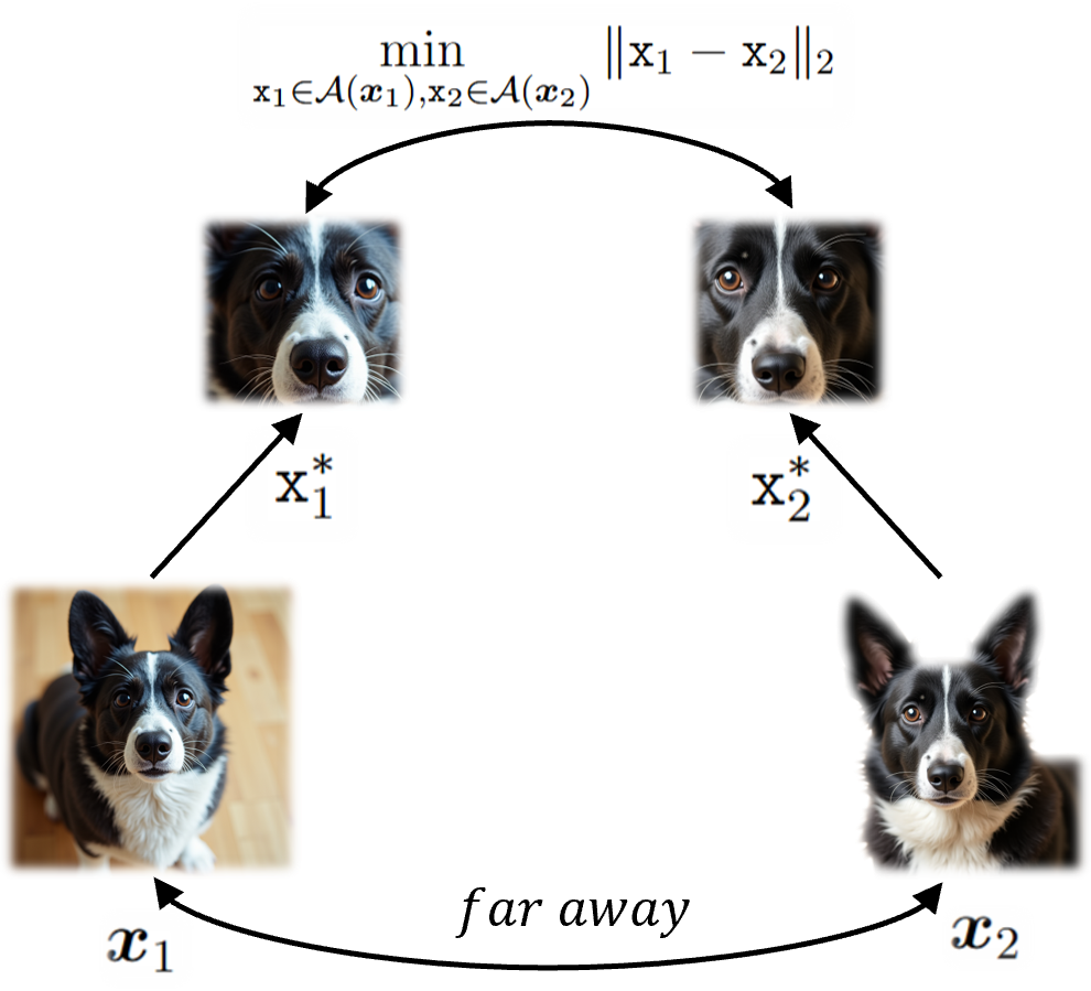
Figure 5: Illustration of $(\sigma,\delta)$-augmentation

We present Figure 5 to illustrate the motivation behind Definition 3. Consider the task of classifying dog and cat. Although the images $\bm{x}_{1}$ and $\bm{x}_{2}$ are semantically similar, their difference, $\|{\bm{x}_{1}-\bm{x}_{2}}\|_{2}$, can be large due to background variations. Through data augmentation, we can find $\mathtt{x}_{1}^{*}\in\mathcal{A}(\bm{x}_{1})$ and $\mathtt{x}_{2}^{*}\in\mathcal{A}(\bm{x}_{2})$ such that $\|{\mathtt{x}_{1}^{*}-\mathtt{x}_{2}^{*}}\|_{2}$ is sufficiently small. In this regard, the quantity $d_{\mathcal{A}}(\bm{x}_{1},\bm{x}_{2}):=\min_{\mathtt{x}_{1}\in\mathcal{A}(\bm{x}_{1}),\mathtt{x}_{2}\in\mathcal{A}(\bm{x}_{2})}\|{\mathtt{x}_{1}-\mathtt{x}_{2}}\|_{2}$ can indeed capture the semantic similarity. Furthermore, the supremum over $C_{T}(k)$, $\sup_{\bm{x}_{T,1},\bm{x}_{T,2}\in C_{T}(k)}d_{\mathcal{A}}(\bm{x}_{T,1},\bm{x}_{T,2})$ serves as a criterion for evaluating the quality of data augmentation. However, problematic pairs $(\breve{\bm{x}}_{T,1},\breve{\bm{x}}_{T,2})$ such that $d_{\mathcal{A}}(\breve{\bm{x}}_{1},\breve{\bm{x}}_{2})$ is significantly larger than that of other pairs, causing the supremum to be disproportionately large, leading to unreliable results. To fix this issue, we replace $C_{T}(k)$ with its subset $\widetilde{C}_{T}(k)$ satisfying condition (i), improving the robustness of the definition. Moreover, condition (iii) implies that the augmentation should be sufficiently effective to correctly recognize the objects that align with the image label. Specifically, consider the image presented in Figure 3, this condition necessitates that the data augmentations can accurately recognize the patch of toilet paper rather than the other objects, as this image has been labeled as toilet paper in ImageNet. A simpler alternative to this condition is to assume that different classes $C_{T}(k)$ are pairwise disjoint, i.e., $\forall i\neq j,C_{T}(i)\cap C_{T}(j)=\emptyset$, which implies $\mathbb{P}_{T}\{\cup_{k=1}^{K}\widetilde{C}_{T}(k)\big{\}}=\sum_{k=1}^{K}\mathbb{P}_{T}\{\widetilde{C}_{T}(k)\}\geq\sigma\sum_{k=1}^{K}\mathbb{P}_{T}\{C_{T}(k)\}=\sigma$. With these, we are now are ready to present the population theorem.

Theorem 1.

Given a $(\sigma,\delta)$-augmentation, if the encoder $f$ with $\|{f}\|_{2}=R$ is $L$-Lipschitz, and if Assumption 1 and 2 hold, then for any $\varepsilon>0$, $\max_{i\neq j}\mu_{T}(i)^{\top}\mu_{T}(j)\lesssim\mathcal{L}(f)+\epsilon_{1}$. Furthermore, if $\max_{i\neq j}\mu_{T}(i)^{\top}\mu_{T}(j)<R^{2}\psi(\sigma,\delta,\varepsilon,f)$, then the downstream misclassification rate of $G_{f}$

$$\mathrm{Err}(G_{f})\leq(1-\sigma)+\mathcal{O}\Big{(}\varepsilon^{-1}\big{\{}\mathcal{L}(f)+\epsilon_{1}+\epsilon_{2}\big{\}}^{\frac{1}{2}}\Big{)},$$

where the specific formulation of $\psi(\sigma,\delta,\varepsilon,f)$ can be found in Lemma 2.

Theorem 1 demonstrates that minimizing the loss function of DM results in a well-separated representation space for downstream task. Specifically, once the quantity $\mu_{T}(i)^{\top}\mu_{T}(j)$ falls below the critical threshold $\psi(\sigma,\delta,\varepsilon,f)$, minimizing $\mathcal{L}(f)$ significantly reduces the downstream misclassification rate. The error bound is composed of three factors: the quality of augmentation $\sigma$, the loss function of DM, $\mathcal{L}(f)$, and the distribution shift $\epsilon_{1},\epsilon_{2}$.

While Theorem 1 highlights the effectiveness of DM, several questions remain unresolved. First, can the sample-level minimizer $\hat{f}_{n_{S}}$ satisfy the conditions of Theorem 1? Second, is it possible to establish an end-to-end error bound for DM to analyze the impact of $n_{S}$ and $n_{T}$ on the misclassification rate, thereby elucidating the success of few-shot learning?

3.2 Sample Theorem

Assumption 3.

Assume there exists a sequence of $(\sigma_{n},\delta_{n})$-augmentations $\mathcal{A}_{n}$ such that both $\sigma_{n}\to 1$ and $\delta_{n}\to 0$.

We note that, in contrast to Assumption 4.3 in Duan et al. (2024), which requires the convergence rate of $\delta_{n}$ to be faster than $\mathcal{O}(n^{-(d+1)/2(\gamma+d+1)})$ for $f^{*}$ in the Hölder class with parameter $\gamma$, our Assumption 3 only requires that $\delta_{n}\to 1$ without any constraint on the convergence rate. Hence, Assumption 3 is notably milder.

Assumption 4.

Assume there exists $\alpha>0$ and $\beta>0$ such that $\epsilon_{1}=\mathcal{O}(n_{S}^{-\alpha})$ and $\epsilon_{2}=\mathcal{O}(n_{S}^{-\beta})$ for sufficiently large $n_{S}$.

This assumption implies that the distribution shift should not be excessive. Intuitively, a model that distinguishes between cats and dogs is largely ineffective for identifying whether a patient is ill based on X-ray images, due to the significant domain shift between the tasks.

Before presenting the final assumption, we introduce Lemma 1, known as Brenier’s theorem in optimal transport theory. Its proof can be found in Theorem 1 of Ball (2004).

Lemma 1 (Existence of Optimal Transport Map).

If $\nu_{1}$ and $\nu_{2}$ are probability measures on $\mathbb{R}^{k}$, $\nu_{2}$ has compact support and $\nu_{1}$ assigns no mass to any set of Hausdorff dimension $(k-1)$, then there exists a optimal transport map $T:\mathbb{R}^{k}\to\mathbb{R}^{k}$ transporting $\nu_{1}$ to $\nu_{2}$, i.e. $T_{\sharp}(\nu_{1})=\nu_{2}$. Moreover, $T$ is bijective.

We now introduce Assumption 5, which justifies that $\mathcal{L}(f^{*})=0$, a crucial step for extending our theory to the sample level. Further details are provided in Section C.5.

Assumption 5.

Suppose there exists a Lipschitz map $f:\mathcal{X}_{S}\to\mathbb{R}^{d^{*}}$ satisfying (i) $f_{\sharp}\mathbb{P}_{S}$ assigns no mass to any set of Hausdorff dimension $(d^{*}-1)$ and (ii) the optimal transport map transporting $f_{\sharp}\mathbb{P}_{S}$ to $\mathbb{P}_{\mathcal{R}}$ is also Lipschitz continuous.

The Lipschitz continuity of optimal transport maps has long been a key yet challenging problem, with numerous studies demonstrating this property under specific classes of distributions (Caffarelli, 2000; Kim and Milman, 2012; Carlier et al., 2024; Fathi et al., 2024). Therefore, Assumption 5 essentially concerns the data distribution, where the variability of $f$ may allow a broad range of distributions to satisfy this condition.

Theorem 2.

Suppose Assumptions 1-5 hold. Set the widths and depths of the encoder and critic networks satisfying $\mathtt{D}_{2}\mathtt{W}_{2}\lesssim\mathtt{D}_{1}\mathtt{W}_{1}=\mathcal{O}\big{(}n_{S}^{-\frac{d}{2d+4}}\big{)}$, and set the augmentation as $\mathcal{A}_{n_{S}}$, then with probability at least $1-\mathcal{O}\big{(}n_{S}^{-\min\{\frac{1}{d+2},\alpha\}}\big{)}-\mathcal{O}\big{(}\frac{1}{\sqrt{\min_{k}n_{T}(k)}}\big{)}$,

$$\mathbb{E}_{\widetilde{\mathcal{D}}_{S}}\big{\{}\mathrm{Err}(G_{\hat{f}_{n_{S}}})\big{\}}\leq\big{(}1-\sigma_{n_{S}}\big{)}+\mathcal{O}\Big{(}n_{S}^{-\min\{\frac{1}{2d+4},\frac{\alpha}{4},\frac{\beta}{4}\}}\Big{)}$$

holds for sufficiently large $n_{S}$.

We defer the proof to Section C. Theorem 2 reveals that appropriately setting the widths and depths of encoder and critic ensures that the downstream misclassification rate of $G_{\hat{f}_{n_{S}}}$ is controlled by the quality of data augmentation $\sigma_{n_{S}}$ and the source sample size, with high probability. The convergence rate of the downstream misclassification rate is jointly determined by the original data dimension $d$ and the extent of the distribution shift, $\alpha$ and $\beta$. This probability approaches $1$ as $n_{S}$ or $n_{T}(k)$ increases. Notably, the convergence rate regarding $\min_{k}n_{T}(k)$ is $1/2$, implying even with a few downstream samples, as long as the unlabeled sample size $n_{S}$ is sufficiently large, the misclassification rate can still be maintained at a sufficiently low level, which coincides with empirical observations in practice.

4 Experiment

The PyTorch implementation of DM can be found in https://github.com/vincen-github/DM.

Method	CIFAR-10		CIFAR-100		STL-10
	Linear	$k$-nn	Linear	$k$-nn	Linear	$k$-nn
Barlow Twins (Zbontar et al., 2021)	83.96	81.18	56.75	47.91	81.41	76.41
SimCLR (Chen et al., 2020a)	90.23	87.57	64.16	53.65	87.44	82.68
Haochen22 (HaoChen et al., 2022)	86.95	82.83	53.75	48.40	81.44	77.31
Vicreg (Bardes et al., 2022)	87.16	85.10	56.63	49.59	84.63	81.13
DM	91.10	88.17	64.49	53.11	88.65	84.21

Table 1: Classification accuracy (top 1) of a linear classifier and a $k$-nearest neighbors classifier ($k=5$) for different loss functions and datasets.

4.1 Experiment details

Datasets

Following prior self-supervised learning works (Chen et al., 2020a; Ermolov et al., 2021; Zbontar et al., 2021; HaoChen et al., 2021; Bardes et al., 2022), we evaluate our method on three widely used image datasets: CIFAR-10 (Krizhevsky, 2009), CIFAR-100 (Krizhevsky, 2009), and STL-10 (Coates et al., 2011). Each dataset is split into three parts: an unsupervised set for training the encoder and critic via DM, a supervised set for training the linear classifier, and a testing set to assess the error.

Experimental Pipeline

During training, we randomly crop and resize images to 32$\times$32 (CIFAR-10, CIFAR-100) or 64$\times$64 (STL-10) before feeding them into the encoder. In the pretraining phase, we use the Adam optimizer to update both the encoder and the projection head based on the unlabeled dataset. After pretraining, the encoder is frozen, and the projection head is removed. We then train a linear classifier on top of the frozen encoder using another Adam optimizer, with the classifier represented as a linear transformation from $\mathbb{R}^{d^{*}}$ to $\mathbb{R}^{K}$. followed by a softmax layer. The classification loss is cross-entropy. We evaluate the classifier’s accuracy on the testing dataset and also report the performance of a $k$-nearest neighbors classifier ($k$=5) without fine-tuning.

Network Architecture

The encoder backbone is ResNet-18 (He et al., 2016), while the critic network consists of three smaller layers, each followed by layer normalization (Ba et al., 2016) and a LeakyReLU activation with a slope of 0.2. The critic’s dimensionality transformation follows $d^{*}\to 128\to d^{*}\to 1$. Notably, an overly complex critic may impair the learned representation’s performance. Following Chen et al. (2020a), we train a projection head alongside the encoder during the self-supervised task. The projection head is a two-layer ReLU network with a hidden size of 1000.

Estimating Mallows’ Distance with Gradient Penalty

Mallow’s distance in Equation (8) involves a minimization problem with the constraint $g\in\mathrm{Lip}(1)$, which is difficult to optimize directly due to the challenging nature of searching the $\mathrm{Lip}(1)$ set. To address this, Gulrajani et al. (2017) reformulate Mallow’s distance in Equation (9) as an unconstrained optimization problem,

$$\mathcal{W}_{\mathrm{gp}}(f,g)=\mathbb{E}_{Z\sim\mathbb{P}_{f}}\big{\{}g(Z)\big{\}}-\mathbb{E}_{\mathcal{R}\sim\mathbb{P}_{\mathcal{R}}}\big{\{}g(\mathcal{R})\big{\}}+\eta\cdot\mathbb{E}_{\bar{X}\sim\mathbb{P}_{\bar{X}}}\Big{[}\big{\{}\big{\|}\nabla_{\bar{X}}g(\bar{X})\big{\|}-1\big{\}}^{2}\Big{]},$$ (19)

where $\eta>0$ is a tuning parameter referred to as the “plenty weight”, typically set to 1 during DM training. Let $U[0,1]$ be the uniform distribution on the interval $[0,1]$ The random variable $\bar{X}\sim\mathbb{P}_{\bar{X}}$ is defined by $\bar{X}=uZ+(1-u)\mathcal{R}$, where $Z\sim\mathbb{P}_{f}$, $\mathcal{R}\sim\mathbb{P}_{\mathcal{R}}$, and $u\sim U[0,1]$. In practice, the encoder is updated at each step, while the critic is updated every five steps.

Hyperparameters

We set $K^{\prime}=384$, $R=1$ and $\epsilon=10^{-3}$ across all datasets. The encoder’s output dimension $d^{*}$ is set to be 384. The learning rates for the encoder and critic are $3\times 10^{-5}$ and $10^{-3}$, respectively, with weight decay of $5\times 10^{-7}$ and $10^{-4}$. A learning rate warm-up is applied for the first 500 iterations of the encoder optimizer. The weight parameter $\lambda$ is set as 1 for all datasets. is set to 1 for all datasets. The batch sizes are 512 for CIFAR-10 and CIFAR-100, and 384 for STL-10, with training for 1000 epochs on the unsupervised dataset. During testing, a linear classifier is trained for 500 epochs using the Adam optimizer with an exponentially decaying learning rate from $10^{-2}$ to $10^{-6}$, and a weight decay of $5\times 10^{-6}$.

Data Augmentations

We randomly extract crops ranging in size from 0.2 to 1.0 of the original area, with aspect ratios varying from 3/4 to 4/3 of the original aspect ratio. Horizontal mirroring is applied with a probability of 0.5. Additionally, color jittering is configured with parameters 0.4, 0.4, 0.4, 0.1 and a probability of 0.8, while grayscaling is applied with a probability of 0.2. During testing, only randomly crop and resize are utilized for evaluation.

Platform

All experiments were conducted using a single Tesla V100 GPU unit. The torch version is 2.2.1+cu118 and the CUDA version is 11.8.

4.2 Ablation Experiment: Finer-Grained Concept

As shown in Figure 4, some samples (e.g., orange and gray points) share similar semantic meaning (both represent “dog”) but are distant in the representation space due to the existence of finer-grained classes (e.g., “black dog” and “orange dog”). Whether self-supervised representation learning methods can effectively capture such subclass structures remains an open question, particularly in real-world applications (HaoChen et al., 2021, 2022; HaoChen and Ma, 2023).

A key distinction between our theoretical framework and experiments lies in the optimization of $\widehat{W}$. In theory, $\widehat{W}$ can be directly calculated, whereas in practice, it is updated via gradient descent. This approach relaxes the constraint $K^{\prime}=K$ discussed in Section 3 and provides greater flexibility. Additionally, $K^{\prime}$ offers significant interpretability, reflecting the number of concepts within the data. Intuitively, as the number of learned concepts were to increase within a certain range, more fine-grained concepts would be captured, and the transferability of the representations would improve. We validate this through the following ablation experiments.

Concept number ($K^{\prime}$)	64	128	256	384	512
Linear	49.83	55.93	61.13	64.49	63.87
$k$-nn	32.73	44.17	51.00	53.11	52.45

Table 2: The influence of concept number on representation performance. All experiments are conducted on CIFAR-100. The parameter $k$ is set to be $5$ and the representation dimension $d^{*}$ is set as $K^{\prime}$.

5 Outlook

Our study offers significant potential for further exploration in self-supervised learning. First, replacing the Mallows’ distance with alternative divergences may yield more efficient representations. Second, as highlighted by Wang and Isola (2020), Awasthi et al. (2022), and Duan et al. (2024), different self-supervised learning losses can lead to distinct structures in the representation space. While analyzing the structure of some existing losses is challenging due to their specialized design, recovering these structures via DM and examining the hyperparameters of the reference distribution may provide valuable insights into their interpretation. Lastly, the condition in Definition 3 represents a crucial factor in advancing self-supervised learning methods. Random augmentation compositions may be too disruptive for handling more complex real-world tasks. How to derive more effective augmentations that align with the requirements in Definition 3 remains an open question for future investigation.

Appendix A Notation List

Given the large number of symbols in this paper, consolidating them in this section offers readers a convenient reference. This structure reduces confusion and enhances comprehension by guiding readers to the first occurrence of each symbol in the relevant sections or equations.

Symbol	Description	Reference
$\mathcal{D}_{S}$	source dataset	Section 2
$\mathcal{D}_{T}$	target dataset	Section 2
$\widetilde{\mathcal{D}}_{S}$	augmentation-reference dataset	Section 2.3
$\widetilde{\mathcal{D}}_{T}$	augmented target dataset	Section 2.4
$C_{S}(k)$	$k$-th source latent class	Section 3.1
$C_{T}(k)$	$k$-th target class	Definition 3
$\widetilde{C}_{T}(k)$	main part of $C_{T}(k)$	Definition 3
$C_{k}$	$k$-th unlabeled reference part	Definition 3
$C_{\mathcal{R}}(k)$	$k$-th labeled reference part	Section 3.1
$n_{T}(k)$	sample size of $k$-th target class	Equation (13)
$n_{S}$	sample size of source dataset	Section 2
$n_{T}$	sample size of target dataset	Section 2
$\mathbb{P}_{S}$	source distribution	Section 2
$\mathbb{P}_{T}$	target distribution	Section 2
$\mathbb{P}_{S}(k)$	distribution conditioned on $X^{S}\in C_{S}(k)$	Section 3.1
$\mathbb{P}_{T}(k)$	distribution conditioned on $Y=k$	Section 3.1
$p_{S}(k)$	probability of $X^{S}\in C^{S}_{k}$	Section 3.1
$p_{T}(k)$	probability of $Y=k$	Section 3.1
$\mu_{S}(k)$	center of $k$-th latent class	Section 3.1
$\mu_{T}(k)$	center of $k$-th target class	Section 2.4
$\mathcal{P}_{i}$	random variable of $i$-th reference part	Equation (6)
$\bm{c}_{i}$	center of $i$-th reference part	Section 2.3
$\epsilon$	range of reference part	Equation (6)
$\epsilon_{1},\epsilon_{2}$	distribution shift	Equation (17)
$K^{\prime}$	number of reference parts	Section 2.3
$K$	the number downstream classes	Section 2
$\mathbb{P}_{\mathcal{R}}$	reference distribution	Section 2.3
$\mathbb{P}_{f}$	representation distribution	Section 2.3
$\mathcal{R}$	random vector of reference	Section 2.3
$R$	range constraint of encoder	Equation (3)
$\mathcal{F}$	feasible set of encoder	Equation (3)
$\mathcal{G}$	feasible set of critic	Equation (8)
$\widehat{\mathcal{F}}$	space for approximating $\mathcal{F}$	Equation (11)
$\widehat{\mathcal{G}}$	space for approximating $\mathcal{G}$	Equation (11)
$f^{*}$	population optimal encoder	Equation (7)
$\hat{f}_{n_{S}}$	empirical optimal encoder	Equation (11)
$L$	Lipschitz constant of encoder	Equation (3)
$Q$	Lipschitz constant of augmentations	Assumption 2
$M$	number of augmentations	Section 2.2
$\mathcal{W}(\mathbb{P}_{f},\mathbb{P}_{\mathcal{R}})$	Mallows’ distance between $\mathbb{P}_{f},\mathbb{P}_{\mathcal{R}}$	Equation (7)
$\mathcal{W}(f,g)$	$\mathbb{E}_{Z\sim\mathbb{P}_{f}}\{g(Z)\}-\mathbb{E}_{\mathcal{R}\sim\mathbb{P}_{\mathcal{R}}}\{g(\mathcal{R})\}$	Equation (2.3)
$\mathcal{L}(f)$	$\mathcal{L}_{\mathrm{align}}(f)+\lambda\cdot\mathcal{W}(\mathbb{P}_{f},\mathbb{P}_{\mathcal{R}})$	Equation (7)
$\mathcal{L}(f,g)$	$\mathcal{L}_{\mathrm{align}}(f)+\lambda\cdot\mathcal{W}(f,g)$	Equation (9)

Table 3: Summary of Symbols

Appendix B Population theorem

The population theorem in this study mainly builds upon the technique used in Huang et al. [2023] and Duan et al. [2024].

Lemma 2.

Given a $(\sigma,\delta)$-augmentation, if the encoder $f$ with $R_{1}\leq\|{f}\|_{2}\leq R_{2}$ is $L$-Lipschitz and

$$\mu_{T}(i)^{\top}\mu_{T}(j)<R_{2}^{2}\psi(\sigma,\delta,\varepsilon,f),$$

holds for any pair of $(i,j)$ with $i\neq j$, then for any $\varepsilon>0$, the downstream misclassification rate of $G_{f}$

$$\text{\rm Err}(G_{f})\leq(1-\sigma)+U_{T}(\varepsilon,f),$$

where $U_{T}(\varepsilon,f)=\mathbb{P}_{T}\big{\{}X_{T}:\sup_{\mathtt{X}_{T,1},\mathtt{X}_{T,2}\sim\mathcal{A}(X_{T})}\|{f(\mathtt{X}_{T,1})-f(\mathtt{X}_{T,2})}\|_{2}>\varepsilon\big{\}}$ and

$$\psi(\sigma,\delta,\varepsilon,f) =\Gamma_{\min}(\sigma,\delta,\varepsilon,f)-\sqrt{2-2\Gamma_{\min}(\sigma,\delta,\varepsilon,f)}-\frac{1}{2}\Big{(}1-\frac{\min_{k}\|{\hat{\mu}_{T}(k)}\|_{2}^{2}}{R_{2}}\Big{)}$$

$$\qquad-\frac{2\max_{k}\|{\hat{\mu}_{T}(k)-\mu_{T}(k)}\|_{2}}{R_{2}},$$ (20)

here $\Gamma_{\min}(\sigma,\delta,\varepsilon,f)$ is given by

$$\Gamma_{\min}(\sigma,\delta,\varepsilon,f)=\begin{cases}(2\sigma-1)-\frac{U_{T}(\varepsilon,f)}{\min_{i}p_{T}(i)}-\Big{(}\sigma-\frac{U_{T}(\varepsilon,f)}{\min_{i}p_{T}(i)}\Big{)}\Big{(}\frac{L\delta}{B}+\frac{2\varepsilon}{B}\Big{)},&R_{1}=R_{2}=R\\ \big{(}\sigma-\frac{U_{T}(\varepsilon,f)}{\min_{i}p_{T}(i)}\big{)}\big{(}1+\big{(}\frac{R_{2}}{R_{1}}\big{)}^{2}-\frac{L\delta}{R_{2}}-\frac{2\varepsilon}{R_{2}}\big{)}-1,&R_{1}<R_{2}.\end{cases}$$

Proof.

For any encoder $f$, let $V_{T}(\varepsilon,f):=\{X_{T}:\sup_{\mathtt{X}_{T,1},\mathtt{X}_{T,2}\sim\mathcal{A}(X_{T})}\|{f(\mathtt{X}_{T,1})-f(\mathtt{X}_{T,2})}\|_{2}\leq\varepsilon\}$, if any $X_{T}\in\widetilde{C}_{T}(1)\cup\cdots\cup\widetilde{C}_{T}(K)\cap V_{T}(\varepsilon,f)$ can be correctly classified by $G_{f}$, it turns out that $\mathrm{Err}(G_{f})$ can be bounded by $(1-\sigma)+U_{T}(\varepsilon,f)$. In fact,

$$\mathrm{Err}(G_{f}) =\mathbb{P}_{T}\big{\{}G_{f}(X_{T})\neq k,Y=k\big{\}}\leq\mathbb{P}_{T}\Big{[}\big{\{}\widetilde{C}_{T}(1)\cup\cdots\cup\widetilde{C}_{T}(K)\cap V_{T}(\varepsilon,f)\big{\}}^{c}\Big{]}$$

$$=\mathbb{P}_{T}\Big{[}\big{(}\widetilde{C}_{T}(1)\cup\cdots\cup\widetilde{C}_{T}(K)\big{)}^{c}\cup\big{\{}V_{T}(\varepsilon,f)\big{\}}^{c}\Big{]}\leq(1-\sigma)+\mathbb{P}_{T}\big{[}\{V_{T}(\varepsilon,f)\}^{c}\big{]}$$

$$=(1-\sigma)+U_{T}(\varepsilon,f),$$

where the last row is due to the fact $U_{T}(\varepsilon,f)=\{V_{T}(\varepsilon,f)\}^{c}$.

Hence it suffices to show for given $1\leq i\leq K$, $X_{T}\in\widetilde{C}_{T}(i)\cap V_{T}(\varepsilon,f)$ can be correctly classified by $G_{f}$ if for any $j\neq i$,

$$\mu_{T}(i)^{\top}\mu_{T}(j)<R_{2}^{2}\psi(\sigma,\delta,\varepsilon,f).$$

To this end, without losing generality, consider the case $i=1$. To turn out $X_{T}\in\widetilde{C}_{T}(1)\cap V_{T}(\varepsilon,f)$ can be correctly classified by $G_{f}$ under given condition, by the definition of $\widetilde{C}_{T}(1)$ and $V_{T}(\varepsilon,f)$, It suffices to show for any $k\neq 1,\|{f(X_{T})-\hat{\mu}_{T}(1)}\|_{2}<\|{f(X_{T})-\hat{\mu}_{T}(k)}\|_{2}$, which is equivalent to

$$f(X_{T})^{\top}\hat{\mu}_{T}(1)-f(X_{T})^{\top}\hat{\mu}_{T}(k)-\Big{(}\frac{1}{2}\|{\hat{\mu}_{T}(1)}\|^{2}_{2}-\frac{1}{2}\|{\hat{\mu}_{T}(k)}\|^{2}_{2}\Big{)}>0.$$ (21)

We will firstly deal with the term $f(X_{T})^{\top}\hat{\mu}_{T}(1)$,

$$f(X_{T})^{\top}\hat{\mu}_{T}(1)=f(X_{T})^{\top}\mu_{T}(1)+f(X_{T})^{\top}\{\hat{\mu}_{T}(1)-\mu_{T}(1)\}$$

$$\geq f(X_{T})^{\top}\mathbb{E}_{(X_{T},Y)\sim\mathbb{P}_{T}}\mathbb{E}_{\mathtt{X}_{T}\sim\mathcal{A}(X_{T})}\{f(\mathtt{X}_{T})|Y=1\}-\|{f(X_{T})}\|_{2}\|{\hat{\mu}_{T}(1)-\mu_{T}(1)}\|_{2}$$

$$\geq\frac{1}{p_{T}(1)}f(X_{T})^{\top}\mathbb{E}_{(X_{T},Y)\sim\mathbb{P}_{T}}\mathbb{E}_{\mathtt{X}_{T}\sim\mathcal{A}(X_{T})}\Big{[}f(\mathtt{X}_{T})\mathbbm{1}\big{\{}X_{T}\in C_{T}(1)\big{\}}\Big{]}-R_{2}\|{\hat{\mu}_{T}(1)-\mu_{T}(1)}\|_{2}$$

$$=\frac{1}{p_{T}(1)}f(X_{T})^{\top}\mathbb{E}_{(X_{T},Y)\sim\mathbb{P}_{T}}\mathbb{E}_{\mathtt{X}_{T}\sim\mathcal{A}(X_{T})}\Big{[}f(\mathtt{X}_{T})\mathbbm{1}\big{\{}X_{T}\in C_{T}(1)\cap\widetilde{C}_{T}(1)\cap V_{T}(\varepsilon,f)\big{\}}\Big{]}$$

$$\qquad+\frac{1}{p_{T}(1)}f(X_{T})^{\top}\mathbb{E}_{(X_{T},Y)\sim\mathbb{P}_{T}}\mathbb{E}_{\mathtt{X}_{T}\sim\mathcal{A}(X_{T})}\Big{[}f(\mathtt{X}_{T})\mathbbm{1}\big{\{}X_{T}\in C_{T}(1)\cap\big{(}\widetilde{C}_{T}(1)\cap V_{T}(\varepsilon,f)\big{)}^{c}\big{\}}\Big{]}$$

$$\qquad-R_{2}\|{\hat{\mu}_{T}(1)-\mu_{T}(1)}\|_{2}$$

$$=\frac{\mathbb{P}_{T}\big{\{}\widetilde{C}_{T}(1)\cap V_{T}(\varepsilon,f)\big{\}}}{p_{T}(1)}f(X_{T})^{\top}\mathbb{E}_{(X_{T},Y)\sim\mathbb{P}_{T}}\mathbb{E}_{\mathtt{X}_{T}\sim\mathcal{A}(X_{T})}\Big{\{}f(\mathtt{X}_{T})\big{|}X_{T}\in\widetilde{C}_{T}(1)\cap V_{T}(\varepsilon,f)\Big{\}}$$

$$\qquad+\frac{1}{p_{T}(1)}\mathbb{E}_{(X_{T},Y)\sim\mathbb{P}_{T}}\Big{[}\mathbb{E}_{\mathtt{X}_{T}\sim\mathcal{A}(X_{T})}\big{\{}f(X_{T})^{\top}f(\mathtt{X}_{T})\big{\}}\mathbbm{1}\big{\{}X_{T}\in C_{T}(1)\backslash\big{(}\widetilde{C}_{T}(1)\cap V_{T}(\varepsilon,f)\big{)}\big{\}}\Big{]}$$

$$\qquad-R_{2}\|{\hat{\mu}_{T}(1)-\mu_{T}(1)}\|_{2}$$

$$\geq\frac{\mathbb{P}_{T}\big{\{}\widetilde{C}_{T}(1)\cap V_{T}(\varepsilon,f)\big{\}}}{p_{T}(1)}f(X_{T})^{\top}\mathbb{E}_{(X_{T},Y)\sim\mathbb{P}_{T}}\mathbb{E}_{\mathtt{X}_{T}\sim\mathcal{A}(X_{T})}\big{\{}f(\mathtt{X}_{T})\big{|}X_{T}\in\widetilde{C}_{T}(1)\cap V_{T}(\varepsilon,f)\big{\}}$$

$$\qquad-\frac{R_{2}^{2}}{p_{T}(1)}\mathbb{P}_{T}\Big{[}C_{T}(1)\backslash\big{\{}\widetilde{C}_{T}(1)\cap V_{T}(\varepsilon,f)\big{\}}\Big{]}-R_{2}\|{\hat{\mu}_{T}(1)-\mu_{T}(1)}\|_{2},$$ (22)

where the second and the third inequalities are both due to the $\|{f}\|_{2}\leq R_{2}$.

Furthermore, we note that

$$\mathbb{P}_{T}\Big{[}C_{T}(1)\backslash\big{\{}\widetilde{C}_{T}(1)\cap V_{T}(\varepsilon,f)\big{\}}\Big{]} =\mathbb{P}_{T}\Big{[}\{C_{T}(1)\backslash\widetilde{C}_{T}(1)\}\cup\big{\{}\widetilde{C}_{T}(1)\cap\big{(}V_{T}(\varepsilon,f)\big{)}^{c}\}\Big{]}$$

$$\leq(1-\sigma)p_{T}(1)+U_{T}(\varepsilon,f),$$ (23)

and

$$\mathbb{P}_{T}\big{\{}\widetilde{C}_{T}(1)\cap V_{T}(\varepsilon,f)\big{\}} =\mathbb{P}_{T}\{C_{T}(1)\}-\mathbb{P}_{T}\Big{[}C_{T}(1)\backslash\big{\{}\widetilde{C}_{T}(1)\cap V_{T}(\varepsilon,f)\big{\}}\Big{]}$$

$$\geq p_{T}(1)-\big{\{}(1-\sigma)p_{T}(1)+U_{T}(\varepsilon,f)\big{\}}$$

$$=\sigma p_{T}(1)-U_{T}(\varepsilon,f).$$ (24)

Plugging (B), (B) into (B) yields

$$f(X_{T})^{\top}\hat{\mu}_{T}(1) \geq\Big{(}\sigma-\frac{U_{T}(\varepsilon,f)}{p_{T}(1)}\Big{)}f(X_{T})^{\top}\mathbb{E}_{(X_{T},Y)\sim\mathbb{P}_{T}}\mathbb{E}_{\mathtt{X}_{T}\sim\mathcal{A}(X_{T})}\big{\{}f(\mathtt{X}_{T})\big{|}X_{T}\in\widetilde{C}_{T}(1)\cap V_{T}(\varepsilon,f)\big{\}}$$

$$\qquad-R_{2}^{2}\Big{(}1-\sigma+\frac{U_{T}(\varepsilon,f)}{p_{T}(1)}\Big{)}-R_{2}\|{\hat{\mu}_{T}(1)-\mu_{T}(1)}\|_{2}.$$ (25)

Notice that $X_{T}\in\widetilde{C}_{T}(1)\cap V_{T}(\varepsilon,f)$. Thus for any $X_{T}^{\prime}\in\widetilde{C}_{T}(1)\cap V_{T}(\varepsilon,f)$, by the definition of $\widetilde{C}_{T}(1)$, we have $\min_{\mathtt{X}_{T}\sim\mathcal{A}(X_{T}),\mathtt{X}_{T}^{\prime}\sim\mathcal{A}(X_{T}^{\prime})}\|{\mathtt{X}_{T}-\mathtt{X}_{T}^{\prime}}\|_{2}\leq\delta$. Further denote $(\mathtt{X}_{T}^{*},\mathtt{X}_{T}^{\prime*})=\arg\min_{\mathtt{X}_{T}\sim\mathcal{A}(X_{T}),\mathtt{X}_{T}^{\prime}\sim\mathcal{A}(\mathtt{X}_{T}^{\prime})}\|{\mathtt{X}_{T}-\mathtt{X}_{T}^{\prime}}\|_{2}$, then $\|{\mathtt{X}_{T}^{*}-\mathtt{X}_{T}^{\prime*}}\|_{2}\leq\delta$, combining $L$-Lipschitz property of $f$ to yield $\|{f(\mathtt{X}_{T}^{*})-f(\mathtt{X}_{T}^{\prime*})}\|_{2}\leq L\|{\mathtt{X}_{T}^{*}-\mathtt{X}_{T}^{\prime*}}\|_{2}\leq L\delta$. Besides that, since $X_{T}^{\prime}\in V_{T}(\varepsilon,f)$, for any $\mathtt{X}_{T}^{\prime}\sim\mathcal{A}(X_{T}^{\prime}),\|{f(\mathtt{X}_{T}^{\prime})-f(\mathtt{X}_{T}^{\prime*})}\|_{2}\leq\varepsilon$. Similarly, as $X_{T}\in V_{T}(\varepsilon,f)$ and $\mathtt{X}_{T},\mathtt{X}_{T}^{*}\sim\mathcal{A}(X_{T})$, we know $\|{f(\mathtt{X}_{T})-f(\mathtt{X}_{T}^{*})}\|_{2}\leq\varepsilon$. Therefore,

$$f(X_{T})^{\top}\mathbb{E}_{(X_{T},Y)\sim\mathbb{P}_{T}}\mathbb{E}_{\mathtt{X}_{T}\sim\mathcal{A}(X_{T})}\big{\{}f(\mathtt{X}_{T})\big{|}X_{T}\in\widetilde{C}_{T}(1)\cap V_{T}(\varepsilon,f)\big{\}}$$

$$=\mathbb{E}_{(X_{T},Y)\sim\mathbb{P}_{T}}\mathbb{E}_{\mathtt{X}_{T}\sim\mathcal{A}(X_{T})}\big{\{}f(X_{T})^{\top}f(\mathtt{X}_{T})\big{|}X_{T}\in\widetilde{C}_{T}(1)\cap V_{T}(\varepsilon,f)\big{\}}$$

$$=\mathbb{E}_{(X_{T},Y)\sim\mathbb{P}_{T}}\mathbb{E}_{\mathtt{X}_{T}\sim\mathcal{A}(X_{T})}\Big{[}f(X_{T})^{\top}\big{\{}f(\mathtt{X}_{T})-f(X_{T}^{\prime})+f(X_{T}^{\prime})\big{\}}\big{|}X_{T}\in\widetilde{C}_{T}(1)\cap V_{T}(\varepsilon,f)\Big{]}$$

$$\geq R_{1}^{2}+\mathbb{E}_{(X_{T},Y)\sim\mathbb{P}_{T}}\mathbb{E}_{\mathtt{X}_{T}\sim\mathcal{A}(X_{T})}\Big{[}f(X_{T})^{\top}\big{\{}f(\mathtt{X}_{T})-f(X_{T}^{\prime})\big{\}}\big{|}X_{T}\in\widetilde{C}_{T}(1)\cap V_{T}(\varepsilon,f)\Big{]}$$

$$=R_{1}^{2}+\mathbb{E}_{(X_{T},Y)\sim\mathbb{P}_{T}}\mathbb{E}_{\mathtt{X}_{T}\sim\mathcal{A}(X_{T})}\Big{[}f(X_{T})^{\top}\big{\{}f(\mathtt{X}_{T})-f(\mathtt{X}_{T}^{*})+f(\mathtt{X}_{T}^{*})-f(\mathtt{X}_{T}^{\prime*})$$

$$\qquad+f(\mathtt{X}_{T}^{\prime*})-f(X_{T}^{\prime})\big{\}}\big{|}X_{T}\in\widetilde{C}_{T}(1)\cap V_{T}(\varepsilon,f)\Big{]}$$

$$\geq R_{1}^{2}-(R_{2}\varepsilon+R_{2}L\delta+R_{2}\varepsilon)$$

$$=R_{1}^{2}-R_{2}(L\delta+2\varepsilon),$$ (26)

where the first inequality is derived from the fact that $\|{f}\|_{2}\geq R_{1}$. Subsequently, plugging (B) to the inequality (B) yields

$$f(X_{T})^{\top}\hat{\mu}_{T}(1) \geq\Big{(}\sigma-\frac{U_{T}(\varepsilon,f)}{p_{T}(1)}\Big{)}f(X_{T})^{\top}\mathop{\mathbb{E}}\limits_{(X_{T},Y)\sim\mathbb{P}_{T}}\mathop{\mathbb{E}}\limits_{\mathtt{X}_{T}\sim\mathcal{A}(X_{T})}\{f(\mathtt{X}_{T})\}-R_{2}^{2}\Big{(}1-\sigma+\frac{U_{T}(\varepsilon,f)}{p_{T}(1)}\Big{)}$$

$$\qquad-R_{2}\|{\hat{\mu}_{T}(1)-\mu_{T}(1)}\|_{2}$$

$$\geq\Big{(}\sigma-\frac{U_{T}(\varepsilon,f)}{p_{T}(1)}\Big{)}\big{(}R_{1}^{2}-R_{2}(L\delta+2\varepsilon)\big{)}-R_{2}^{2}\Big{(}1-\sigma+\frac{U_{T}(\varepsilon,f)}{p_{T}(1)}\Big{)}$$

$$\qquad-R_{2}\|{\hat{\mu}_{T}(1)-\mu_{T}(1)}\|_{2}$$

$$=R_{2}^{2}\Gamma_{1}(\sigma,\delta,\varepsilon,f)-R_{2}\|{\hat{\mu}_{T}(1)-\mu_{T}(1)}\|_{2},$$ (27)

where $\Gamma_{1}(\sigma,\delta,\varepsilon,f)$ is defined as

$$\Gamma_{1}(\sigma,\delta,\varepsilon,f)=\begin{cases}(2\sigma-1)-\frac{U_{T}(\varepsilon,f)}{p_{T}(1)}-\Big{(}\sigma-\frac{U_{T}(\varepsilon,f)}{p_{T}(1)}\Big{)}\Big{(}\frac{L\delta}{R_{2}}+\frac{2\varepsilon}{R_{2}}\Big{)},&R_{1}=R_{2}=R\\ \big{(}\sigma-\frac{U_{T}(\varepsilon,f)}{p_{T}(1)}\big{)}\big{(}1+\big{(}\frac{R_{2}}{R_{1}}\big{)}^{2}-\frac{L\delta}{R_{2}}-\frac{2\varepsilon}{R_{2}}\big{)}-1.&R_{1}<R_{2}\end{cases}$$

As for the term $f(X_{T})^{\top}\hat{\mu}_{T}(k)$ in (21), we note that similar deduction process as above can also turns out $f(X_{T})^{\top}\mu_{T}(1)\geq R_{2}^{2}\Gamma_{1}(\sigma,\delta,\varepsilon,f)$, along with the fact: any $1\leq k\leq K$, $\|\mu_{T}(k)\|_{2}=\|\mathbb{E}_{(X_{T},Y)\sim\mathbb{P}_{T}}\mathbb{E}_{\mathtt{X}_{T}\sim\mathcal{A}(X_{T})}\{f(\mathtt{X}_{T})|Y=k\}\|_{2}\leq\mathbb{E}_{(X_{T},Y)\sim\mathbb{P}_{T}}\mathbb{E}_{\mathtt{X}_{T}\sim\mathcal{A}(X_{T})}\{\|f(\mathtt{X}_{T})\|_{2}|Y=k\}\leq R_{2}$, we have

$$f(X_{T})^{\top}\hat{\mu}_{T}(k)\leq f(X_{T})^{\top}\mu_{T}(k)+f(X_{T})^{\top}(\hat{\mu}_{T}(k)-\mu_{T}(k))$$

$$\leq f(X_{T})^{\top}\mu_{T}(k)+\|{f(X_{T})}\|_{2}\|{\hat{\mu}_{T}(k)-\mu_{T}(k)}\|_{2}$$

$$\leq f(X_{T})^{\top}\mu_{T}(k)+R_{2}\|{\hat{\mu}_{T}(k)-\mu_{T}(k)}\|_{2}$$

$$=(f(X_{T})-\mu_{T}(1))^{\top}\mu_{T}(k)+\mu_{T}(1)^{\top}\mu_{T}(k)+R_{2}\|{\hat{\mu}_{T}(k)-\mu_{T}(k)}\|_{2}$$

$$\leq\|{f(X_{T})-\mu_{T}(1)}\|_{2}\cdot\|{\mu_{T}(k)}\|_{2}+\mu_{T}(1)^{\top}\mu_{T}(k)+R_{2}\|{\hat{\mu}_{T}(k)-\mu_{T}(k)}\|_{2}$$

$$\leq R_{2}\sqrt{\|{f(X_{T})}\|^{2}_{2}-2f(X_{T})^{\top}\mu_{T}(1)+\|{\mu_{T}(1)}\|_{2}^{2}}+\mu_{T}(1)^{\top}\mu_{T}(k)+R_{2}\|{\hat{\mu}_{T}(k)-\mu_{T}(k)}\|_{2}$$

$$\leq R_{2}\sqrt{2R_{2}^{2}-2f(X_{T})^{\top}\mu_{T}(1)}+\mu_{T}(1)^{\top}\mu_{T}(k)+R_{2}\|{\hat{\mu}_{T}(k)-\mu_{T}(k)}\|_{2}$$

$$\leq R_{2}\sqrt{2R_{2}^{2}-2R_{2}^{2}\Gamma_{1}(\sigma,\delta,\varepsilon,f)}+\mu_{T}(1)^{\top}\mu_{T}(k)+R_{2}\|{\hat{\mu}_{T}(k)-\mu_{T}(k)}\|_{2}$$

$$=\sqrt{2}R_{2}^{2}\sqrt{1-\Gamma_{1}(\sigma,\delta,\varepsilon,f)}+\mu_{T}(1)^{\top}\mu_{T}(k)+R_{2}\|{\hat{\mu}_{T}(k)-\mu_{T}(k)}\|_{2}.$$ (28)

Plugging (B) and (B) into (21) concludes

$$f(X_{T})^{\top}\hat{\mu}_{T}(1)-f(X_{T})^{\top}\hat{\mu}_{T}(k)-\Big{(}\frac{1}{2}\|{\hat{\mu}_{T}(1)}\|_{2}^{2}-\frac{1}{2}\|{\hat{\mu}_{T}(k)}\|^{2}\Big{)}$$

$$=f(X_{T})^{\top}\hat{\mu}_{T}(1)-f(X_{T})^{\top}\hat{\mu}_{T}(k)-\frac{1}{2}\|{\hat{\mu}_{T}(1)}\|^{2}_{2}+\frac{1}{2}\|{\hat{\mu}_{T}(k)}\|^{2}_{2}$$

$$\geq f(X_{T})^{\top}\hat{\mu}_{T}(1)-f(X_{T})^{\top}\hat{\mu}_{T}(k)-\frac{1}{2}R_{2}^{2}+\frac{1}{2}\min_{k}\|{\hat{\mu}_{T}(k)}\|_{2}^{2}$$

$$=f(X_{T})^{\top}\hat{\mu}_{T}(1)-f(X_{T})^{\top}\hat{\mu}_{T}(k)-\frac{1}{2}R_{2}^{2}\big{(}1-\min_{k}\|{\hat{\mu}_{T}(k)}\|_{2}^{2}/R_{2}^{2}\big{)}$$

$$\geq R_{2}^{2}\Gamma_{1}(\sigma,\delta,\varepsilon,f)-R_{2}\|{\hat{\mu}_{T}(1)-\mu_{T}(1)}\|_{2}-\sqrt{2}R_{2}^{2}\sqrt{1-\Gamma_{1}(\sigma,\delta,\varepsilon,f)}$$

$$\qquad-\mu_{T}(1)^{\top}\mu_{T}(k)-R_{2}\|{\hat{\mu}_{T}(k)-\mu_{T}(k)}\|_{2}-\frac{1}{2}R_{2}^{2}\big{(}1-\min_{k}\|{\hat{\mu}_{T}(k)}\|_{2}^{2}/R_{2}^{2}\big{)}>0,$$

where the last inequality follows from the condition provided in Lemma 2. ∎

Lemma 3.

Given a $(\sigma,\delta)$-augmentation, if the encoder $f$ with $R_{1}\leq\|{f}\|_{2}\leq R_{2}$ is $L$-Lipschitz continuous, then for any $\varepsilon>0$,

$$U_{T}^{2}(\varepsilon,f)\lesssim\varepsilon^{-2}\big{\{}\mathcal{L}_{\mathrm{align}}(f)+\epsilon_{1}+\epsilon_{2}\big{\}},$$ (29)

and

$$\max_{i\neq j}\mu_{T}(i)^{\top}\mu_{T}(j)\lesssim\mathcal{W}(\mathbb{P}_{f},\mathbb{P}_{T})+\epsilon_{1}.$$ (30)

Proof.

The inequality in (30) has been established according to (18). Therefore, we will focus on proving (29) in this lemma. Since the distribution on $\mathcal{A}$ is uniform distribution, we have

$$\mathbb{E}_{\mathtt{X}_{T,1},\mathtt{X}_{T,2}\sim\mathcal{A}(X_{T})}\big{\|}f(\mathtt{X}_{T,1})-f(\mathtt{X}_{T,2})\big{\|}_{2}=\frac{1}{M^{2}}\sum_{i=1}^{M}\sum_{j=1}^{M}\big{\|}f\big{(}A_{i}(X_{T})\big{)}-f\big{(}A_{j}(X_{T})\big{)}\big{\|}_{2}.$$

Hence,

$$\sup_{\mathtt{X}_{T,1},\mathtt{X}_{T,2}\sim\mathcal{A}(X_{T})}\big{\|}f(\mathtt{X}_{T,1})-f(\mathtt{X}_{T,2})\big{\|}_{2} =\sup_{i,j}\big{\|}f\big{(}A_{i}(X_{T})\big{)}-f\big{(}A_{j}(X_{T})\big{)}\big{\|}_{2}$$

$$\leq\sum_{i=1}^{M}\sum_{j=1}^{M}\big{\|}f\big{(}A_{i}(X_{T})\big{)}-f\big{(}A_{j}(X_{T})\big{)}\big{\|}_{2}$$

$$=M^{2}\mathbb{E}_{\mathtt{X}_{T,1},\mathtt{X}_{T,2}\sim\mathcal{A}(X_{T})}\|{f(\mathtt{X}_{T,1})-f(\mathtt{X}_{T,2})}\|_{2},$$

which implies that

$$\Big{\{}X_{T}:\sup_{\mathtt{X}_{T,1},\mathtt{X}_{T,2}\sim\mathcal{A}(X_{T})}\|{f(\mathtt{X}_{T,1})-f(\mathtt{X}_{T,2})}\|_{2}>\varepsilon\Big{\}}\subseteq\Big{\{}X_{T}:\mathop{\mathbb{E}}_{\mathtt{X}_{T,1},\mathtt{X}_{T,2}\sim\mathcal{A}(X_{T})}\|{f(\mathtt{X}_{T,1})-f(\mathtt{X}_{T,2})}\|_{2}>\frac{\varepsilon}{M^{2}}\Big{\}}.$$

Recall the definition $U_{T}(\varepsilon,f)=\mathbb{P}_{T}\{X_{T}:\sup_{\mathtt{X}_{T,1},\mathtt{X}_{T,2}\sim\mathcal{A}(X_{T})}\|{f(\mathtt{X}_{T,1})-f(\mathtt{X}_{T,2})}\|_{2}>\varepsilon\big{\}}$, by Markov inequality, we know that

$$U^{2}_{T}(\varepsilon,f) \leq\mathbb{P}^{2}_{T}\Big{(}\mathbb{E}_{\mathtt{X}_{T,1},\mathtt{X}_{T,2}\sim\mathcal{A}(X_{T})}\big{\|}f(\mathtt{X}_{T,1})-f(\mathtt{X}_{T,2})\big{\|}_{2}>\frac{\varepsilon}{M^{2}}\Big{)}$$

$$\leq\Big{(}\frac{\mathbb{E}_{(X_{T},Y)\sim\mathbb{P}_{T}}\mathbb{E}_{\mathtt{X}_{T,1},\mathtt{X}_{T,2}\sim\mathcal{A}(X_{T})}\big{\|}f(\mathtt{X}_{T,1})-f(\mathtt{X}_{T,2})\big{\|}_{2}}{\frac{\varepsilon}{M^{2}}}\Big{)}^{2}$$

$$\leq\frac{\mathbb{E}_{(X_{T},Y)\sim\mathbb{P}_{T}}\mathbb{E}_{\mathtt{X}_{T,1},\mathtt{X}_{T,2}\sim\mathcal{A}(X_{T})}\big{\|}f(\mathtt{X}_{T,1})-f(\mathtt{X}_{T,2})\big{\|}^{2}_{2}}{\frac{\varepsilon^{2}}{M^{4}}}$$

$$\lesssim\varepsilon^{-2}\mathbb{E}_{(X_{T},Y)\sim\mathbb{P}_{T}}\mathbb{E}_{\mathtt{X}_{T,1},\mathtt{X}_{T,2}\sim\mathcal{A}(X_{T})}\big{\|}f(\mathtt{X}_{T,1})-f(\mathtt{X}_{T,2})\big{\|}^{2}_{2}.$$ (31)

Moreover,

$$\mathop{\mathbb{E}}_{(X_{T},Y)\sim\mathbb{P}_{T}}\mathop{\mathbb{E}}_{\mathtt{X}_{T,1},\mathtt{X}_{T,2}\sim\mathcal{A}(X_{T})}\big{\|}f(\mathtt{X}_{T,1})-f(\mathtt{X}_{T,2})\big{\|}_{2}^{2}$$

$$=\mathop{\mathbb{E}}_{X_{S}\sim\mathbb{P}_{S}}\mathop{\mathbb{E}}_{\mathtt{X}_{S,1},\mathtt{X}_{S,2}\sim\mathcal{A}(X_{S})}\big{\|}f(\mathtt{X}_{S,1})-f(\mathtt{X}_{S,2})\big{\|}_{2}^{2}+\mathop{\mathbb{E}}_{(X_{T},Y)\sim\mathbb{P}_{T}}\mathop{\mathbb{E}}_{\mathtt{X}_{T,1},\mathtt{X}_{T,2}\sim\mathcal{A}(X_{T})}\big{\|}f(\mathtt{X}_{T,1})-f(\mathtt{X}_{T,2})\big{\|}_{2}^{2}$$

$$\qquad-\mathop{\mathbb{E}}_{X_{S}\sim\mathbb{P}_{S}}\mathop{\mathbb{E}}_{\mathtt{X}_{S,1},\mathtt{X}_{S,2}\sim\mathcal{A}(X_{S})}\big{\|}f(\mathtt{X}_{S,1})-f(\mathtt{X}_{S,2})\big{\|}_{2}^{2}$$

$$=\mathop{\mathbb{E}}_{X_{S}\sim\mathbb{P}_{S}}\mathop{\mathbb{E}}_{\mathtt{X}_{S,1},\mathtt{X}_{S,2}\sim\mathcal{A}(X_{S})}\big{\|}f(\mathtt{X}_{S,1})-f(\mathtt{X}_{S,2})\big{\|}_{2}^{2}+\frac{1}{M^{2}}\sum_{i,j}\Big{\{}\mathop{\mathbb{E}}_{(X_{T},Y)\sim\mathbb{P}_{T}}\big{\|}f\big{(}A_{i}(X_{T})\big{)}-f\big{(}A_{j}(X_{T})\big{)}\big{\|}_{2}^{2}$$

$$\qquad-\mathop{\mathbb{E}}_{X_{S}\sim\mathbb{P}_{S}}\big{\|}f(A_{i}(X_{S}))-f(A_{j}(X_{S}))\big{\|}_{2}^{2}\Big{\}}$$

$$=\mathcal{L}_{\mathrm{align}}(f)+\frac{1}{M^{2}}\sum_{i=1}^{M}\sum_{j=1}^{M}\sum_{l=1}^{d^{*}}\Big{[}\mathbb{E}_{(X_{T},Y)\sim\mathbb{P}_{T}}\big{\{}f_{l}(A_{i}(X_{T}))-f_{l}(A_{j}(X_{T}))\big{\}}^{2}$$

$$\qquad-\mathbb{E}_{X_{S}\sim\mathbb{P}_{S}}\big{\{}f_{l}\big{(}A_{i}(X_{S})\big{)}-f_{l}\big{(}A_{j}(X_{S})\big{)}\big{\}}^{2}\Big{]}.$$ (32)

Since for all $i\in[m],j\in[m]$ and $l\in[d^{*}]$, we have

$$\mathbb{E}_{(X_{T},Y)\sim\mathbb{P}_{T}}\big{\{}f_{l}\big{(}A_{i}(X_{T})\big{)}-f_{l}\big{(}A_{j}(X_{T})\big{)}\big{\}}^{2}-\mathbb{E}_{X_{S}\sim\mathbb{P}_{S}}\big{\{}f_{l}\big{(}A_{i}(X_{S})\big{)}-f_{l}\big{(}A_{j}(X_{S})\big{)}\big{\}}^{2}$$

$$=\sum_{k=1}^{K}\Big{[}p_{T}(k)\mathop{\mathbb{E}}_{(X_{T},Y)\sim\mathbb{P}_{T}}\big{\{}f_{l}(A_{i}(X_{T}))-f_{l}(A_{j}(X_{T}))|Y=k\big{\}}^{2}$$

$$\qquad-p_{S}(k)\mathop{\mathbb{E}}_{X_{S}\sim\mathbb{P}_{S}}\big{\{}f_{l}\big{(}A_{i}(X_{S})\big{)}-f_{l}\big{(}A_{j}(X_{S})\big{)}\big{|}X_{S}\in C_{S}(k)\big{\}}^{2}\Big{]}$$

$$=\sum_{k=1}^{K}\Big{[}p_{T}(k)\Big{\{}\mathop{\mathbb{E}}_{(X_{T},Y)\sim\mathbb{P}_{T}}\big{\{}f_{l}\big{(}A_{i}(X_{T})\big{)}-f_{l}\big{(}A_{j}(X_{T})\big{)}\big{|}Y=k\big{\}}^{2}$$

$$\qquad-\mathop{\mathbb{E}}_{X_{S}\sim\mathbb{P}_{S}}\underbrace{\big{\{}f_{l}\big{(}A_{i}(X_{S})\big{)}-f_{l}\big{(}A_{j}(X_{S})\big{)}\big{|}X_{S}\in C_{S}(k)\big{\}}^{2}}_{h(X_{S})}\Big{\}}$$

$$\qquad+\big{\{}p_{T}(k)-p_{S}(k)\big{\}}\mathop{\mathbb{E}}_{X_{S}\sim\mathbb{P}_{S}}\big{\{}f_{l}\big{(}A_{i}(X_{S})\big{)}-f_{l}\big{(}A_{j}(X_{S})\big{)}\big{|}X_{S}\in C_{S}(k)\big{\}}^{2}\Big{]}$$

$$\lesssim\epsilon_{1}+\epsilon_{2},$$ (33)

where the last inequality arises from $\epsilon_{2}=\max_{k}|{p_{S}(k)-p_{T}(k)}|$ and $\epsilon_{1}=\max_{k}\mathcal{W}(\mathbb{P}_{S}(k),\mathbb{P}_{T}(k))$, $\epsilon_{2}=\max_{k}|{p_{S}(k)-p_{T}(k)}|$, along with the dual formulation of Mallows’ distance (5). In fact, since $f$ and any $A\in\mathcal{A}$ are Lipschitz continuous, and given that fact $R_{1}\leq\|{f}\|_{2}\leq R_{2}$, it follows that $h$ is also a Lipschitz function.

Combining (B) (B) (B) yields $U_{T}^{2}(\varepsilon,f)\lesssim\varepsilon^{-2}\big{(}\mathcal{L}_{\mathrm{align}}(f)+\epsilon_{1}+\epsilon_{2}\big{)}$. ∎

Next we represent Theorem 1 and give out its proof.

Theorem 3 (General version of Theorem 1).

Given a $(\sigma,\delta)$-augmentation, if the encoder $f$ with $R_{1}\leq\|{f}\|_{2}\leq R_{2}$ is $L$-Lipschitz and Assumption 1, 2 both hold, then for any $\varepsilon>0$, $\max_{i\neq j}\mu_{T}(i)^{\top}\mu_{T}(j)\lesssim\mathcal{L}(f)+\epsilon_{1}$. Furthermore, if $\max_{i\neq j}\mu_{T}(i)^{\top}\mu_{T}(j)<R_{2}^{2}\psi(\sigma,\delta,\varepsilon,f)$, then the downstream misclassification rate of $G_{f}$

$$\mathrm{Err}(G_{f})\leq(1-\sigma)+\mathcal{O}\Big{(}\varepsilon^{-1}\big{\{}\mathcal{L}(f)+\epsilon_{1}+\epsilon_{2}\big{\}}^{\frac{1}{2}}\Big{)},$$

Proof.

Combining Lemma 2 and Lemma 3 yields this result. It is evident that Theorem 1 is a direct conclusion when setting $R_{1}=R_{2}=R$. ∎

Appendix C Sample Theorem

The sample theorem in this study mainly draws on the technique used in Duan et al. [2024].

C.1 Error Decomposition

Note that $\mathcal{L}(f)=\sup_{g\in\mathcal{G}}\mathcal{L}(f,g)$, define the stochastic error $\mathcal{E}_{\mathrm{sta}}$, the encoder approximation error $\mathcal{E}_{\mathcal{F}}$ and the discriminator approximation error, $\mathcal{E}_{\mathcal{G}}$ respectively as follows

$$\mathcal{E}_{\mathrm{sta}}:=\sup_{f\in\widehat{\mathcal{F}},g\in\widehat{\mathcal{G}}}|{\mathcal{L}(f,g)-\widehat{\mathcal{L}}(f,g)}|,$$

$$\mathcal{E}_{\mathcal{F}}:=\inf_{f\in\widehat{\mathcal{F}}}\{\mathcal{L}(f)-\mathcal{L}(f^{*})\},$$

$$\mathcal{E}_{\mathcal{G}}:=\sup_{f\in\widehat{\mathcal{F}}}\big{|}\sup_{g\in\mathcal{G}}\mathcal{W}(f,g)-\sup_{g\in\widehat{\mathcal{G}}}\mathcal{W}(f,g)\big{|}.$$

Then we have following relationship.

Lemma 4.

$\mathcal{L}(\hat{f}_{n_{S}})\leq\mathcal{L}(f^{*})+2\mathcal{E}_{\mathrm{sta}}+\mathcal{E}_{\mathcal{F}}+2\mathcal{E}_{\mathcal{G}}$.

Proof.

For any $f\in\widehat{\mathcal{F}}$,

$$\mathcal{L}(\hat{f}_{n_{S}}) =\big{\{}\mathcal{L}(\hat{f}_{n_{S}})-\sup_{g\in\widehat{\mathcal{G}}}\mathcal{L}(\hat{f}_{n_{S}},g)\big{\}}+\big{\{}\sup_{g\in\widehat{\mathcal{G}}}\mathcal{L}(\hat{f}_{n_{S}},g)-\sup_{g\in\widehat{\mathcal{G}}}\widehat{\mathcal{L}}(\hat{f}_{n_{S}},g)\big{\}}$$

$$\qquad+\big{\{}\sup_{g\in\widehat{\mathcal{G}}}\widehat{\mathcal{L}}(\hat{f}_{n_{S}},g)-\sup_{g\in\widehat{\mathcal{G}}}\widehat{\mathcal{L}}(f,g)\big{\}}+\big{\{}\sup_{g\in\widehat{\mathcal{G}}}\widehat{\mathcal{L}}(f,g)-\sup_{g\in\widehat{\mathcal{G}}}\mathcal{L}(f,g)\big{\}}$$

$$\qquad+\big{\{}\sup_{g\in\widehat{\mathcal{G}}}\mathcal{L}(f,g)-\mathcal{L}(f)\big{\}}+\big{\{}\mathcal{L}(f)-\mathcal{L}(f^{*})\big{\}}+\mathcal{L}(f^{*})$$

For the second term and the forth term, we can conclude

$$\sup_{g\in\widehat{\mathcal{G}}}\mathcal{L}(\hat{f}_{n_{S}},g)-\sup_{g\in\widehat{\mathcal{G}}}\widehat{\mathcal{L}}(\hat{f}_{n_{S}},g)\leq\sup_{g\in\widehat{\mathcal{G}}}\{\mathcal{L}(\hat{f}_{n_{S}},g)-\widehat{\mathcal{L}}(\hat{f}_{n_{S}},g)\}\leq\mathcal{E}_{\mathrm{sta}}$$

and

$$\sup_{g\in\widehat{\mathcal{G}}}\widehat{\mathcal{L}}(f,g)-\sup_{g\in\widehat{\mathcal{G}}}\mathcal{L}(f,g) \leq\sup_{g\in\widehat{\mathcal{G}}}\{\widehat{\mathcal{L}}(f,g)-\mathcal{L}(f,g)\}\leq\mathcal{E}_{\mathrm{sta}}$$

The first and the fifth terms both can be bounded $\mathcal{E}_{\mathcal{G}}$. For the first term:

$$\mathcal{L}(\hat{f}_{n_{S}})-\sup_{g\in\widehat{\mathcal{G}}}\mathcal{L}(\hat{f}_{n_{S}},g) \leq\sup_{f\in\widehat{\mathcal{F}}}\{\mathcal{L}(f)-\sup_{g\in\widehat{\mathcal{G}}}\mathcal{L}(f,g)\}=\sup_{f\in\widehat{\mathcal{F}}}\{\sup_{g\in\mathcal{G}}\mathcal{W}(f,g)-\sup_{g\in\widehat{\mathcal{G}}}\mathcal{W}(f,g)\}$$

$$\leq\sup_{f\in\widehat{\mathcal{F}}}\big{|}\sup_{g\in\mathcal{G}}\mathcal{W}(f,g)-\sup_{g\in\widehat{\mathcal{G}}}\mathcal{W}(f,g)\big{|}=\mathcal{E}_{\mathcal{G}}.$$

Similar for the fifth term,

$$\sup_{g\in\widehat{\mathcal{G}}}\mathcal{L}(f,g)-\mathcal{L}(f) \leq\sup_{f\in\widehat{\mathcal{F}}}\{\sup_{g\in\widehat{\mathcal{G}}}\mathcal{L}(f,g)-\mathcal{L}(f)\}=\sup_{f\in\widehat{\mathcal{F}}}\{\sup_{g\in\widehat{\mathcal{G}}}\mathcal{W}(f,g)-\sup_{g\in\mathcal{G}}\mathcal{W}(f,g)\}$$

$$\leq\sup_{f\in\widehat{\mathcal{F}}}|{\sup_{g\in\widehat{\mathcal{G}}}\mathcal{W}(f,g)-\sup_{g\in\mathcal{G}}\mathcal{W}(f,g)}|=\mathcal{E}_{\mathcal{G}}$$

Finally, taking infimum over all $f\in\widehat{\mathcal{F}}$ yields

$$\mathcal{L}(\hat{f}_{n_{S}})\leq\mathcal{L}(f^{*})+2\mathcal{E}_{\mathrm{sta}}+\mathcal{E}_{\mathcal{F}}+2\mathcal{E}_{\mathcal{G}}.$$

∎

C.2 The Stochastic Error

Let $\ell(\bm{v}_{1},\bm{v}_{2},v_{3},v_{4},v_{5})=\|{\bm{v}_{1}-\bm{v}_{2}}\|_{2}^{2}+v_{3}-\frac{1}{2}\{v_{4}+v_{5}\}$, where $\bm{v}_{1},\bm{v}_{2}\in\mathbb{R}^{d^{*}}$ and $v_{3},v_{4},v_{5}\in\mathbb{R}$. It immediately follows that

$$\widehat{\mathcal{L}}(f,g)=\frac{1}{n_{S}}\sum_{i=1}^{n_{S}}\ell\big{(}f(\mathtt{X}^{(i)}_{S,1}),f(\mathtt{X}^{(i)}_{S,2}),g(\mathcal{R}^{(i)}),g(f(\mathtt{X}^{(i)}_{S,1})),g(f(\mathtt{X}^{(i)}_{S,2}))\big{)}.$$

Let $\widetilde{\mathcal{D}}^{\prime}_{S}=\{(\mathtt{X}_{S,1}^{\prime(i)},\mathtt{X}_{S,2}^{\prime(i)},\mathcal{R}^{\prime}_{i}):1\leq i\leq n_{S}\}$ be a random copy of $\widetilde{\mathcal{D}}_{S}$, which follows that

$$\mathcal{L}(f,g)=\frac{1}{n_{S}}\sum_{i=1}^{n_{S}}\mathbb{E}_{\widetilde{\mathcal{D}}^{\prime}_{s}}\big{\{}\ell\big{(}f(\mathtt{X}_{S,1}^{\prime(i)}),f(\mathtt{X}_{S,2}^{\prime(i)}),g(\mathcal{R}^{\prime}_{i}),g(f(\mathtt{X}_{S,1}^{\prime(i)})),g(f(\mathtt{X}_{S,2}^{\prime(i)}))\big{)}\big{\}}$$

Plugging this equation into the definition of $\mathcal{E}_{\mathrm{sta}}$ yields

$$\mathbb{E}_{\widetilde{\mathcal{D}}_{S}}\big{\{}\mathcal{E}_{\mathrm{sta}}\big{\}} =\mathbb{E}_{\widetilde{\mathcal{D}}_{S}}\big{\{}\sup_{f\in\widehat{\mathcal{F}},g\in\widehat{\mathcal{G}}}|{\mathcal{L}(f,g)-\widehat{\mathcal{L}}(f,g)}|\big{\}}$$

$$\leq\mathbb{E}_{\widetilde{\mathcal{D}}_{S}}\Big{[}\sup_{(f,g)\in\widehat{\mathcal{F}}\times\widehat{\mathcal{G}}}\Big{|}\frac{1}{n_{S}}\sum_{i=1}^{n_{S}}\mathbb{E}_{\widetilde{\mathcal{D}}^{\prime}_{S}}\big{\{}\ell\big{(}f(\mathtt{X}_{S,1}^{\prime(i)}),f(\mathtt{X}_{S,2}^{\prime(i)}),g(\mathcal{R}^{\prime}_{i}),g(f(\mathtt{X}_{S,1}^{\prime(i)})),g(f(\mathtt{X}_{S,2}^{\prime(i)}))\big{)}\big{\}}$$

$$\qquad-\frac{1}{n_{S}}\sum_{i=1}^{n_{S}}\ell\big{(}f(\mathtt{X}_{S,1}^{(i)}),f(\mathtt{X}_{S,2}^{(i)}),g(\mathcal{R}^{(i)}),g(f(\mathtt{X}_{S,1}^{(i)})),g(f(\mathtt{X}_{S,2}^{(i)}))\big{)}\Big{|}\Big{]}$$

$$\leq\mathbb{E}_{\widetilde{\mathcal{D}}_{S},\widetilde{\mathcal{D}}_{S}^{\prime}}\Big{\{}\sup_{(f,g)\in\widehat{\mathcal{F}}\times\widehat{\mathcal{G}}}\Big{|}\frac{1}{n_{S}}\sum_{i=1}^{n_{S}}\ell\big{(}f(\mathtt{X}_{S,1}^{\prime(i)}),f(\mathtt{X}_{S,2}^{\prime(i)}),g(\mathcal{R}^{(i)}),g(f(\mathtt{X}_{S,1}^{\prime(i)})),g(f(\mathtt{X}_{S,2}^{\prime(i)}))\big{)}$$

$$\qquad-\ell\big{(}f(\mathtt{X}_{S,1}^{(i)}),f(\mathtt{X}_{S,2}^{(i)}),g(\mathcal{R}^{(i)}),g(f(\mathtt{X}_{S,1}^{(i)})),g(f(\mathtt{X}_{S,2}^{(i)}))\big{)}\Big{|}\Big{\}}$$

$$\leq\mathbb{E}_{\widetilde{\mathcal{D}}_{S},\widetilde{\mathcal{D}}_{S}^{\prime},\bm{\xi}}\Big{\{}\sup_{(f,g)\in\widehat{\mathcal{F}}\times\widehat{\mathcal{G}}}\Big{|}\frac{1}{n_{S}}\sum_{i=1}^{n_{S}}\xi_{i}\Big{(}\ell\big{(}f(\mathtt{X}_{S,1}^{\prime(i)}),f(\mathtt{X}_{S,2}^{\prime(i)}),g(\mathcal{R}^{(i)}),g(f(\mathtt{X}_{S,1}^{\prime(i)})),g(f(\mathtt{X}_{S,2}^{\prime(i)}))\big{)}$$

$$\qquad-\ell\big{(}f(\mathtt{X}_{S,1}^{(i)}),f(\mathtt{X}_{S,2}^{(i)}),g(\mathcal{R}^{(i)}),g(f(\mathtt{X}_{S,1}^{(i)})),g(f(\mathtt{X}_{S,2}^{(i)}))\big{)}\Big{)}\Big{|}\Big{\}},$$

where the last inequality stems from the standard randomization techniques in empirical process theory, as detailed in Giné and Nickl [2016]. Moreover, since $\widetilde{\mathcal{D}}^{\prime}_{S}$ is a random copy of $\mathcal{D}_{S}$, we have

$$\mathbb{E}_{\widetilde{\mathcal{D}}_{S}}\big{\{}\mathcal{E}_{\mathrm{sta}}\big{\}} \leq 2\mathbb{E}_{\widetilde{\mathcal{D}}_{S},\bm{\xi}}\Big{\{}\sup_{(f,g)\in\widehat{\mathcal{F}}\times\widehat{\mathcal{G}}}\Big{|}\frac{1}{n_{S}}\sum_{i=1}^{n_{S}}\xi_{i}\ell\big{(}f(\mathtt{X}_{S,1}^{(i)}),f(\mathtt{X}_{S,2}^{(i)}),g(\mathcal{R}^{(i)}),g(f(\mathtt{X}_{S,1}^{(i)})),g(f(\mathtt{X}_{S,2}^{(i)}))\big{)}\Big{|}\Big{\}}$$

$$\lesssim\mathbb{E}_{\widetilde{\mathcal{D}}_{S},\bm{\xi}}\Big{[}\sup_{(f,g)\in\widehat{\mathcal{F}}\times\widehat{\mathcal{G}}}\Big{|}\frac{1}{n_{S}}\sum_{i=1}^{n_{S}}\sum_{j=1}^{d^{*}}\big{\{}\xi_{i,j,1}f_{j}(\mathtt{X}_{S,1}^{(i)})+\xi_{i,j,2}f_{j}(\mathtt{X}_{S,2}^{(i)})\big{\}}+\xi_{i,1}g(\mathcal{R}^{(i)})$$

$$\qquad+\xi_{i,2}g(f(\mathtt{X}_{S,1}^{(i)}))+\xi_{i,3}g(f(\mathtt{X}_{S,2}^{(i)}))\Big{|}\Big{]}$$

$$\lesssim\mathbb{E}_{\widetilde{\mathcal{D}}_{S},\bm{\xi}}\Big{\{}\sup_{f\in\widehat{\mathcal{F}}}\Big{|}\frac{1}{n_{S}}\sum_{i=1}^{n_{S}}\sum_{j=1}^{d^{*}}\xi_{i,j}f_{j}(\mathtt{X}_{S,1}^{(i)})\Big{|}\Big{\}}+\mathbb{E}_{\widetilde{\mathcal{D}}_{S},\bm{\xi}}\Big{\{}\sup_{g\in\widehat{\mathcal{G}}}\Big{|}\frac{1}{n_{S}}\sum_{i=1}^{n_{S}}\xi_{i}g(\mathcal{R}^{(i)})\Big{|}\Big{\}}$$

$$\qquad+\mathbb{E}_{\widetilde{\mathcal{D}}_{S},\bm{\xi}}\Big{\{}\sup_{(f,g)\in\widehat{\mathcal{F}}\times\widehat{\mathcal{G}}}\Big{|}\frac{1}{n_{S}}\sum_{i=1}^{n_{S}}\xi_{i}g(f(\mathtt{X}_{S,1}^{(i)}))\Big{|}\Big{\}},$$ (34)

where the second inequality follows from the vector-contraction principle, derived by combining Maurer [2016] with Theorem 3.2.1 in Giné and Nickl [2016].

Lemma 5 (Vector-contraction principle).

Let $\mathcal{X}$ be any set, $(x_{1},\ldots,x_{n})\in\mathcal{X}^{n}$, let $\mathcal{H}$ be a class of functions $f:\mathcal{X}\rightarrow\ell_{2}$ and let $h_{i}:\ell_{2}\rightarrow\mathbb{R}$ have Lipschitz norm $L^{\prime}$. Then

$$\mathbb{E}\sup_{f\in\mathcal{H}}\Big{|}\sum_{i}\xi_{i}h_{i}(f(x_{i}))\Big{|}\leq 2\sqrt{2}L^{\prime}\mathbb{E}\sup_{f\in\mathcal{H}}\Big{|}\sum_{i,k}\xi_{ik}f_{k}(x_{i})\Big{|},$$

where $\xi_{ik}$ is an independent doubly indexed Rademacher sequence and $f_{k}(x_{i})$ is the $k$-th component of $f(x_{i})$.

To deal with three terms concluded in (C.2), it is necessary to introduce several definitions and lemmas below.

Definition 4 (Covering number).

Let $n\in\mathbb{N}$, $\mathcal{S}\subseteq\mathbb{R}^{n}$, and $\rho>0$. A set $\mathcal{N}\subseteq\mathcal{S}$ is called a $\varrho$-net of $\mathcal{S}$ with respect to a metric $d$ if for every $\bm{u}\in\mathcal{S}$, there exists $\bm{v}\in\mathcal{N}$ such that $d(\bm{u},\bm{v})\leq\varrho$. The covering number of $\mathcal{S}$ is defined as

$$\mathcal{N}(\varrho,\mathcal{S},d):=\min\big{\{}|{\mathcal{Q}}|:\mathcal{Q}\text{ is an $\varrho$-cover of }\mathcal{S}\big{\}},$$

where $|{\mathcal{Q}}|$ is the cardinality of the set $\mathcal{Q}$.

Definition 5 (Uniform covering number).

Let $\mathcal{H}$ be a class of functions from $\mathcal{X}$ to $\mathbb{R}$. Given a sequence $x=(x_{1},x_{2},\ldots,x_{k})\in\mathcal{X}^{k}$, define $\mathcal{H}_{|_{x}}$ be the subset of $\mathbb{R}^{n}$ given by $\mathcal{H}_{|_{x}}=\{(f(x_{1}),f(x_{2}),\ldots,f(x_{k})):f\in\mathcal{H}\}$. For a positive number $\varrho$, the uniform covering number is given by

$$\mathcal{N}_{\infty}(\varrho,\mathcal{H},k)=\max\big{\{}\mathcal{N}(\varrho,\mathcal{H}_{|_{x}},d):x\in\mathcal{X}^{k}\big{\}}.$$

Lemma 6 (Lemma 10.5 of Anthony and Bartlett [1999]).

Let $\mathcal{H}$ is a class of functions from $\mathcal{X}$ to $\mathbb{R}$. For any $\varrho>0$ and $x\in\mathcal{X}^{k}$, we have the following inequality for the covering numbers:

$$\mathcal{N}(\varrho,\mathcal{H}_{|_{x}},d_{1})\leq\mathcal{N}(\varrho,\mathcal{H}_{|_{x}},d_{2})\leq\mathcal{N}(\varrho,\mathcal{H}_{|_{x}},d_{\infty}),$$

where $d_{1}(\bm{x},\bm{y}):=\frac{1}{n}\sum_{i=1}^{n}|{x_{i}-y_{i}}|,d_{2}(\bm{x},\bm{y}):=\big{(}\frac{1}{n}\sum_{i=1}^{n}(x_{i}-y_{i})^{2}\big{)}^{1/2}$ and $d_{\infty}(\bm{x},\bm{y}):=\max_{1\leq i\leq n}|x_{i}-y_{i}|$.

Definition 6 (Sub-Gaussian process).

A centred stochastic process $X(t),t\in T$, is sub-Gaussian with respect to a distance or pseudo-distance $d$ on $T$ if its increments satisfy the sub-Gaussian inequality, that is, if

$$\mathbb{E}[e^{\varsigma\{X(t)-X(s)\}}]\leq e^{\varsigma^{2}d^{2}(s,t)/2},\varsigma\in\mathbb{R},s,t\in T.$$

The following lemma are derived from Theorem 2.3.7 in Giné and Nickl [2016]:

Lemma 7 (Dudley’s entropy integral).

Let $(T,d)$ be a separable pseudo-metric space, and let $X(t),t\in T$, be a sub-Gaussian process relative to $d$. Then

$$\mathbb{E}\sup_{t\in T}|{X(t)}|\leq\mathbb{E}|{X(t_{0})}|+4\sqrt{2}\int_{0}^{D/2}\sqrt{\log 2\mathcal{N}(\varrho,T,d)}d\varrho.$$

where $t_{0}$ is any point in $T$ and $D$ is the diameter of $(T,d)$.

Proof.

It is remarkable to note that the essence of the entropy condition $\int_{0}^{\infty}\log\mathcal{N}(\rho,T,d)d\varrho<\infty$ in the proof of Theorem 2.3.7 in Giné and Nickl [2016] is to establish the separability of $(T,d)$. ∎

Based on Lemma 7 and (C.2), we can conclude

$$\mathbb{E}_{\widetilde{\mathcal{D}}_{S}}\big{\{}\mathcal{E}_{\mathrm{sta}}\big{\}} \lesssim\frac{1}{\sqrt{n_{S}}}\mathbb{E}_{\widetilde{\mathcal{D}}_{S}}\Big{\{}\int_{0}^{\mathtt{B}_{1}}\sqrt{\log 2\mathcal{N}\big{(}\varrho,\mathcal{NN}_{d,1}(\mathtt{W}_{1},\mathtt{D}_{1},\mathtt{B}_{1})_{|_{\{\mathtt{X}^{(i)}_{S,1}\}_{i=1}^{n_{S}}}},d_{2}\big{)}}d\varrho$$

$$\qquad+\int_{0}^{\mathtt{B}_{2}}\sqrt{\log 2\mathcal{N}\big{(}\varrho,\mathcal{NN}_{d^{*},1}(\mathtt{W}_{2},\mathtt{D}_{2},\mathtt{B}_{2})_{|_{\{\mathcal{R}^{(i)}\}_{i=1}^{n_{S}}}},d_{2}\big{)}}d\varrho$$

$$\qquad+\int_{0}^{\mathtt{B}_{2}}\sqrt{\log 2\mathcal{N}\big{(}\varrho,\mathcal{NN}_{d,1}(\max\{\mathtt{W}_{1},\mathtt{W}_{2}\},\mathtt{D}_{1}+\mathtt{D}_{2},\mathtt{B}_{2})_{|_{\{\mathcal{R}^{(i)}\}_{i=1}^{n_{S}}}},d_{2}\big{)}}d\varrho\Big{\}}.$$ (35)

We exemplify the first term in (C.2). By the fact that $f\in\widehat{\mathcal{F}}\Rightarrow f_{j}\in\mathcal{NN}_{d,1}(\mathtt{W}_{1},\mathtt{D}_{1},\mathtt{B}_{1})$ for any $1\leq j\leq d^{*}$, along with Fubini theorem, we have

$$\mathbb{E}_{\widetilde{\mathcal{D}}_{S},\bm{\xi}}\Big{\{}\sup_{f\in\widehat{\mathcal{F}}}\Big{|}\frac{1}{n_{S}}\sum_{i=1}^{n_{S}}\sum_{j=1}^{d^{*}}\xi_{i,j}f_{j}(\mathtt{X}_{S,1}^{(i)})\Big{|}\Big{\}}\leq d^{*}\mathbb{E}_{\widetilde{\mathcal{D}}_{S},\bm{\xi}}\Big{[}\mathbb{E}_{\bm{\xi}}\Big{\{}\sup_{f\in\mathcal{NN}_{d,1}(\mathtt{W}_{1},\mathtt{D}_{1},\mathtt{B}_{1})}\Big{|}\frac{1}{n_{S}}\sum_{i=1}^{n_{S}}\xi_{i}f(\mathtt{X}_{S,1}^{(i)})\Big{|}\Big{\}}$$

$$=d^{*}\mathbb{E}_{\widetilde{\mathcal{D}}_{S}}\Big{[}\mathbb{E}_{\bm{\xi}}\Big{\{}\sup_{f\in\mathcal{NN}_{d,1}(\mathtt{W}_{1},\mathtt{D}_{1},\mathtt{B}_{1})}\Big{|}\frac{1}{n_{S}}\sum_{i=1}^{n_{S}}\xi_{i}f(\mathtt{X}_{S,1}^{(i)})\Big{|}\Big{|}\mathtt{X}_{S,1}^{(i)},1\leq i\leq n_{S}\Big{\}}\Big{]}.$$

Therefore, it suffices to show

$$\mathbb{E}_{\bm{\xi}}\Big{\{}\sup_{f\in\mathcal{NN}_{d,1}(\mathtt{W}_{1},\mathtt{D}_{1},\mathtt{B}_{1})}\Big{|}\frac{1}{\sqrt{n_{S}}}\sum_{i=1}^{n_{S}}\xi_{i}f(\mathtt{X}_{S,1}^{(i)})\Big{|}\Big{|}\widetilde{\mathcal{D}}_{S}\Big{\}}\leq\int_{0}^{\mathtt{B}_{1}}\sqrt{\log 2\mathcal{N}\big{(}\varrho,\mathcal{NN}_{d,1}(\mathtt{W}_{1},\mathtt{D}_{1},\mathtt{B}_{1})_{|_{\{\mathtt{X}^{(i)}_{S,1}\}_{i=1}^{n_{S}}}},d_{2}\big{)}}d\varrho.$$

In fact, conditioned on $\widetilde{\mathcal{D}}_{S}$, which implies that $\mathtt{X}_{S,1}^{(i)},1\leq i\leq n_{S}$ are fixed, the stochastic process $\{\frac{1}{\sqrt{n_{S}}}\sum_{i=1}^{n_{S}}\xi_{i}f(\mathtt{X}_{S,1}^{(i)}):f\in\mathcal{NN}_{d,1}(\mathtt{W}_{1},\mathtt{D}_{1},\mathtt{B_{1}})\}$ is a sub-Gaussian process, as $\xi_{i},1\leq i\leq n_{S}$ are independent Rademacher variables (see page 40 in Giné and Nickl [2016]). Let $f_{|_{\{\mathtt{X}_{S,1}^{(i)}\}_{i=1}^{n_{S}}}}=(f(\mathtt{X}_{S,1}^{(1)}),\ldots,f(\mathtt{X}_{S,1}^{(n_{S})}))\in\mathbb{R}^{n_{S}}$ for any $f\in\mathcal{NN}_{d,1}(\mathtt{W}_{1},\mathtt{D}_{1},\mathtt{B}_{1})$, and define the distance on the index set $\mathcal{NN}_{d,1}(\mathtt{W}_{1},\mathtt{D}_{1},\mathtt{B}_{1})$ as

$$d_{\mathcal{NN}}(f_{1},f_{2}) :=\sqrt{\mathbb{E}\Big{\{}\Big{|}\frac{1}{\sqrt{n_{S}}}\sum_{i=1}^{n_{S}}\xi_{i}f_{1}(\mathtt{X}_{S,1}^{(i)})-\frac{1}{\sqrt{n_{S}}}\sum_{i=1}^{n_{S}}\xi_{i}f_{2}(\mathtt{X}_{S,1}^{(i)})\Big{|}\Big{\}}}$$

$$=\sqrt{\frac{1}{n_{S}}\sum_{i=1}^{n_{S}}\big{(}f_{1}(\mathtt{X}_{S,1}^{(i)})-f_{2}(\mathtt{X}_{S,1}^{(i)})\big{)}^{2}}=d_{2}({f_{1}}_{|_{\{\mathtt{X}_{S,1}^{(i)}\}_{i=1}^{n_{S}}}},{f_{2}}_{|_{\{\mathtt{X}_{S,1}^{(i)}\}_{i=1}^{n_{S}}}}),$$

we know that $(\mathcal{NN}_{d,1}(\mathtt{W}_{1},\mathtt{D}_{1},\mathtt{B}_{1})_{|_{\{\mathtt{X}^{(i)}_{S,1}\}_{i=1}^{n_{S}}}},d_{2})$ is a separable subset of $\mathbb{R}^{n_{S}}$ due to the existence of networks with rational parameters, satisfying the condition of Lemma 7. Let $f_{\bm{0}}\in\mathcal{NN}_{d,1}(\mathtt{W}_{1},\mathtt{D}_{1},\mathtt{B}_{1})$ be the network with all zero parameters. Setting $t_{0}$ in Lemma 7 as $f_{\bm{0}}$ yields $\mathbb{E}|{X(t_{0})}|=0$. Furthermore, for any $f\in\mathcal{NN}_{d,1}(\mathtt{W}_{1},\mathtt{D}_{1},\mathtt{B}_{1})$:

$$d_{\mathcal{NN}}(f,f_{\bm{0}})=d_{2}(f_{|_{\{\mathtt{X}_{S,1}^{(i)}\}_{i=1}^{n_{S}}}},{f_{\bm{0}}}_{|_{\{\mathtt{X}_{S,1}^{(i)}\}_{i=1}^{n_{S}}}})=\sqrt{\frac{1}{n_{S}}\sum_{i=1}^{n_{S}}f^{2}(X_{S,1}^{(i)})}\leq\mathtt{B}_{1},$$

hence the triangular inequality immediately follows that $D/2\leq\mathtt{B}_{1}$. Combining all facts turns out what we desire. The second and the third terms in C.2 can be obtained similarly.

We now introduce several definitions and lemmas to address the terms in (C.2).

Definition 7 (VC-dimension).

Let $\mathcal{H}$ denote a class of functions from $\mathcal{X}$ to $\{0,1\}$. For any non-negative integer $m$, we define the growth function of $\mathcal{H}$ as

$$\Pi_{\mathcal{H}}(m):=\max_{x_{1},\ldots,x_{m}\in\mathcal{X}}\big{|}\{(h(x_{1}),\ldots,h(x_{m})):h\in\mathcal{H}\}\big{|}.$$

If $|{\{(h(x_{1}),\ldots,h(x_{m})):h\in\mathcal{H}\}}|=2^{m}$, we say $\mathcal{H}$ shatters the set $\{x_{1},\ldots,x_{m}\}$. The Vapnik-Chervonenkis dimension of $\mathcal{H}$, denoted $\mathrm{VCdim}(\mathcal{H})$, is the size of the largest shattered set, i.e. the largest $m$ such that $\Pi_{\mathcal{H}}(m)=2^{m}$. If there is no largest $m$, we define $\mathrm{VCdim}(\mathcal{H})=\infty$. Moreover, for a class $\mathcal{H}$ of real-valued functions, we may define $\mathrm{VCdim}(\mathcal{H}):=\mathrm{VCdim}(\mathrm{sgn}(\mathcal{H}))$, where $\{\mathrm{sgn}(f):f\in\mathcal{H}\}$ and $\mathrm{sgn}(x)=\mathbbm{1}\{x>0\}$.

Definition 8 (pseudodimension).

Let $\mathcal{H}$ be a class of functions from $\mathcal{X}$ to $\mathbb{R}$. The pseudodimension of $\mathcal{H}$, written $\mathrm{Pdim}(\mathcal{H})$, is the largest integer $m$ for which there exists $(x_{1},\ldots,x_{m},y_{1},\ldots,y_{m})\in\mathcal{X}^{m}\times\mathbb{R}^{m}$ such that for any $(b_{1},\ldots,b_{m})\in\{0,1\}^{m}$ there exists $f\in\mathcal{H}$ such that $\forall i:f(x_{i})>y_{i}\Leftrightarrow b_{i}=1$.

Lemma 8 (Theorem 12.2 in Bartlett et al. [2019]).

Let $\mathcal{H}$ be a set of real functions from a domain $\mathcal{X}$ to the bounded interval $[0,\mathtt{B}]$. Then for any $\varrho>0$, the uniform covering number

$$\mathcal{N}_{\infty}(\varrho,\mathcal{H},m)\leq\sum_{i=1}^{\mathrm{Pdim}(\mathcal{H})}\dbinom{m}{i}\dbinom{\mathtt{B}}{\varrho}^{i},$$

which is less than $\big{(}em\mathtt{B}/(\varrho\mathrm{Pdim}(\mathcal{H}))\big{)}^{\mathrm{Pdim}(\mathcal{H})}$ for $m\geq\mathrm{Pdim}(\mathcal{H})$.

Lemma 9 (Theorem 14.1 in Anthony and Bartlett [1999]).

For any $\mathtt{d},\mathtt{W},\mathtt{D}\in\mathbb{N}$,

$$\mathrm{Pdim}\big{(}\mathcal{NN}_{d,1}(\mathtt{W},\mathtt{L})\big{)}\leq\mathrm{VCdim}\big{(}\mathcal{NN}_{d,1}(\mathtt{W},\mathtt{L})\big{)}.$$

Lemma 10 (Theorem 6 in Bartlett et al. [2019]).

For any $\mathtt{d},\mathtt{W},\mathtt{D}\in\mathbb{N}$, let $\mathtt{S}$ be the total number of parameters of $\mathcal{NN}_{\mathtt{d},1}(\mathtt{W},\mathtt{D})$, we have $\mathrm{VCdim}\big{(}\mathcal{NN}_{\mathtt{d},1}(\mathtt{W},\mathtt{D})\big{)}\lesssim\mathtt{D}\mathtt{S}\log_{2}\mathtt{S}$.

Let $\mathcal{NN}_{d_{1},d_{2}}(\mathtt{W},\mathtt{D})$ be the ReLU network class without the constraint $\sup_{\bm{x}\in\mathbb{R}^{p}}\|f_{\bm{\theta}}(\bm{x})\|_{\infty}\leq\mathtt{B}$ in Definition 2, it immediately follows that $\mathcal{NN}_{d_{1},d_{2}}(\mathtt{W},\mathtt{D},\mathtt{B})\subseteq\mathcal{NN}(\mathtt{W},\mathtt{D})$, implying following Lemma

Lemma 11.

For any $\mathtt{d},\mathtt{W},\mathtt{D}\in\mathbb{N}$, we have $\mathrm{Pdim}\big{(}\mathcal{NN}_{\mathtt{d},1}(\mathtt{W},\mathtt{D},\mathtt{B})\big{)}\leq\mathrm{Pdim}\big{(}\mathcal{NN}_{\mathtt{d},1}(\mathtt{W},\mathtt{D})\big{)}$.

Following above preliminaries, we are now further processing (C.2).

$$\mathbb{E}_{\widetilde{\mathcal{D}}_{S}}\big{\{}\mathcal{E}_{\mathrm{sta}}\big{\}} \lesssim\frac{1}{\sqrt{n_{S}}}\mathbb{E}_{\widetilde{\mathcal{D}}_{S}}\Big{\{}\int_{0}^{\mathtt{B}_{1}}\sqrt{\log 2\mathcal{N}\big{(}\varrho,\mathcal{NN}_{d,1}(\mathtt{W}_{1},\mathtt{D}_{1},\mathtt{B}_{1})_{|_{\{\mathtt{X}^{(i)}_{S,1}\}_{i=1}^{n_{S}}}},d_{2}\big{)}}d\varrho$$

$$\qquad+\int_{0}^{\mathtt{B}_{2}}\sqrt{\log 2\mathcal{N}\big{(}\varrho,\mathcal{NN}_{d^{*},1}(\mathtt{W}_{2},\mathtt{D}_{2},\mathtt{B}_{2})_{|_{\{\mathcal{R}^{(i)}\}_{i=1}^{n_{S}}}},d_{2}\big{)}}d\varrho$$

$$\qquad+\int_{0}^{\mathtt{B}_{2}}\sqrt{\log 2\mathcal{N}\big{(}\varrho,\mathcal{NN}_{d,1}(\max\{\mathtt{W}_{1},\mathtt{W}_{2}\},\mathtt{D}_{1}+\mathtt{D}_{2},\mathtt{B}_{2})_{|_{\{\mathcal{R}^{(i)}\}_{i=1}^{n_{S}}}},d_{2}\big{)}}d\varrho\Big{\}}$$

$$\leq\frac{1}{\sqrt{n_{S}}}\mathbb{E}_{\widetilde{\mathcal{D}}_{S}}\Big{\{}\int_{0}^{\mathtt{B}_{1}}\sqrt{\log 2\mathcal{N}\big{(}\varrho,\mathcal{NN}_{d,1}(\mathtt{W}_{1},\mathtt{D}_{1},\mathtt{B}_{1})_{|_{\{\mathtt{X}^{(i)}_{S,1}\}_{i=1}^{n_{S}}}},d_{\infty}\big{)}}d\varrho$$

$$\qquad+\int_{0}^{\mathtt{B}_{2}}\sqrt{\log 2\mathcal{N}\big{(}\varrho,\mathcal{NN}_{d^{*},1}(\mathtt{W}_{2},\mathtt{D}_{2},\mathtt{B}_{2})_{|_{\{\mathcal{R}^{(i)}\}_{i=1}^{n_{S}}}},d_{\infty}\big{)}}d\varrho$$

$$\qquad+\int_{0}^{\mathtt{B}_{2}}\sqrt{\log 2\mathcal{N}\big{(}\varrho,\mathcal{NN}_{d,1}(\max\{\mathtt{W}_{1},\mathtt{W}_{2}\},\mathtt{D}_{1}+\mathtt{D}_{2},\mathtt{B}_{2})_{|_{\{\mathcal{R}^{(i)}\}_{i=1}^{n_{S}}}},d_{\infty}\big{)}}d\varrho\Big{\}}$$ (Lemma 6)

$$\leq\frac{1}{\sqrt{n_{S}}}\Big{\{}\int_{0}^{\mathtt{B}_{1}}\sqrt{\log 2\mathcal{N}_{\infty}\big{(}\varrho,\mathcal{NN}_{d,1}(\mathtt{W}_{1},\mathtt{D}_{1},\mathtt{B}_{1}),n_{S}\big{)}}d\varrho$$

$$\qquad+\int_{0}^{\mathtt{B}_{2}}\sqrt{\log 2\mathcal{N}_{\infty}\big{(}\varrho,\mathcal{NN}_{d^{*},1}(\mathtt{W}_{2},\mathtt{D}_{2},\mathtt{B}_{2}),n_{S}\big{)}}d\varrho$$

$$\qquad+\int_{0}^{\mathtt{B}_{2}}\sqrt{\log 2\mathcal{N}_{\infty}\big{(}\varrho,\mathcal{NN}_{d,1}(\max\{\mathtt{W}_{1},\mathtt{W}_{2}\},\mathtt{D}_{1}+\mathtt{D}_{2},\mathtt{B}_{2}),n_{S}\big{)}}d\varrho\Big{\}}$$ (Definition 5)

$$\lesssim\Big{(}\frac{\mathrm{Pdim}(\mathcal{NN}_{d,1}\big{(}\mathtt{W}_{1},\mathtt{D}_{1})\big{)}\log n_{S}}{n_{S}}\Big{)}^{1/2}+\Big{(}\frac{\mathrm{Pdim}(\mathcal{NN}_{d^{*},1}\big{(}\mathtt{W}_{2},\mathtt{D}_{2})\big{)}\log n_{S}}{n_{S}}\Big{)}^{1/2}$$

$$\qquad+\Big{(}\frac{\mathrm{Pdim}(\mathcal{NN}_{d,1}\big{(}\max\{\mathtt{W}_{1},\mathtt{W}_{2}\},\mathtt{D}_{1}+\mathtt{D}_{2})\big{)}\log n_{S}}{n_{S}}\Big{)}^{1/2}$$ (Lemma 8 and 11)

$$\lesssim\Big{(}\frac{\mathrm{VCdim}(\mathcal{NN}_{d,1}\big{(}\mathtt{W}_{1},\mathtt{D}_{1})\big{)}\log n_{S}}{n_{S}}\Big{)}^{1/2}+\Big{(}\frac{\mathrm{VCdim}(\mathcal{NN}_{d^{*},1}\big{(}\mathtt{W}_{2},\mathtt{D}_{2})\big{)}\log n_{S}}{n_{S}}\Big{)}^{1/2}$$

$$\qquad+\Big{(}\frac{\mathrm{VCdim}(\mathcal{NN}_{d,1}\big{(}\max\{\mathtt{W}_{1},\mathtt{W}_{2}\},\mathtt{D}_{1}+\mathtt{D}_{2})\big{)}\log n_{S}}{n_{S}}\Big{)}^{1/2}$$ (Lemma 9)

$$\leq\mathcal{O}\Big{(}\sqrt{\frac{(\mathtt{D}_{1}+\mathtt{D}_{2})^{2}\max\{\mathtt{W_{1}},\mathtt{W}_{2}\}^{2}}{n_{S}}}\Big{)} \mathtt{S}\leq\mathtt{W}^{2}\mathtt{D}$$ (Lemma 10 and )

$$\lesssim\frac{\mathtt{D}_{1}\mathtt{W_{1}}}{\sqrt{n_{S}}}. \mathtt{W}_{1}\geq\mathtt{W}_{2} \mathtt{D}_{1}\geq\mathtt{D}_{2}$$ ( and )

We ignore the logarithmic term when deriving the penultimate inequality, as its impact on polynomial growth is negligible.

C.3 The Approximation Error

In this section, we aim to determine the upper bounds for $\mathcal{E}_{\mathcal{F}}$ and $\mathcal{E}_{\mathcal{G}}$, following the approach outlined in Yang et al. [2023] and Gao et al. [2024]. To this end, we need to introduce serval definitions and lemmas in advance. Let $d\in\mathbb{N}$ and $U$ be an open subset of $\mathbb{R}^{d}$. We denote $L^{\infty}(U)$ as the standard Lebesgue space on $U$ with $L^{\infty}$ norm.

Definition 9 (Sobolev space).

Let $n\in\{0\}\cup\mathbb{N}$, the Sobolev space $W^{n,\infty}(U)$ is defined by

$$W^{n,\infty}(U):=\{f\in L^{\infty}(U):D^{\bm{\alpha}}f\in L^{\infty}(U)\text{ for all }\bm{\alpha}\in\mathbb{N}_{0}^{d}\text{ with }\|{\bm{\alpha}}\|_{1}\leq n\}.$$

Moreover, for any $f\in W^{n,\infty}(U)$, we define the Sobolev norm $\|{\cdot}\|_{W^{n,\infty}(U)}$ by

$$\|{f}\|_{W^{n,\infty}(U)}:=\max_{0\leq\|{\bm{\alpha}}\|_{1}\leq n}\|{D^{\bm{\alpha}}f}\|_{L^{\infty}(U)}.$$

Lemma 12 (Characterization of $W^{1,\infty}$ in Evans [2010]).

Let $U$ be open and bounded, with $\partial U$ of class $C^{1}$. Then $f:U\to\mathbb{R}$ is Lipschitz continuous if and only if $f\in W^{1,\infty}(U)$

Lemma 13 (Corollary B.2 in Gao et al. [2024]).

For any $f\in W^{1,\infty}((0,1)^{d})$ such that $\|f\|_{W^{1,\infty}((0,1)^{d})}<\infty$, and $\mathtt{N},\mathtt{L}\in\mathbb{N}$, there exists a function $f_{\bm{\theta}}$ implemented by a deep ReLU network with width $\widetilde{\mathcal{O}}(\mathtt{N})$, depth $\widetilde{\mathcal{O}}(\mathtt{L})$ and $\mathtt{B}\geq\|{f}\|_{\infty}$ such that $\|f_{\bm{\theta}}\|_{W^{1,\infty}((0,1))^{d}}\lesssim\|f\|_{W^{1,\infty}((0,1)^{d})}$ and

$$\|{f_{\bm{\theta}}-f}\|_{L^{\infty}([0,1]^{d})}\lesssim\|{f}\|_{W^{1,\infty}((0,1)^{d})}(\mathtt{N}\mathtt{L})^{-2/d}.$$

C.3.1 The Encoder Approximation Error $\mathcal{E}_{\mathcal{F}}$

Lemma 13 and Lemma 12 together demonstrate that the approximation capacity of $\mathcal{NN}_{d,1}(\mathtt{W},\mathtt{D},\mathtt{B})$ to Lipschitz functions can be made arbitrarily precise by increasing the scale of the neural network. Consequently, the function. $\hat{f}_{n_{S}}$ retains the property $R_{1}\leq\|{\hat{f}_{n_{S}}}\|_{2}\leq R_{2}$ for some constants $R_{1}$ and $R_{2}$ close to $R$, allowing us to directly apply Theorem 3.

Recall the $\mathcal{L}(f)$ is defined as follow:

$$\mathcal{L}(f)=\mathop{\mathbb{E}}_{X_{S}\sim\mathbb{P}_{S}}\mathop{\mathbb{E}}_{\mathtt{X}_{S,1},\mathtt{X}_{S,2}\sim\mathcal{A}(X_{S})}\Big{\|}f(\mathtt{X}_{S,1})-f(\mathtt{X}_{S,2})\Big{\|}_{2}^{2}+\lambda\sup_{g\in\mathcal{G}}\mathop{\mathbb{E}}_{Z\sim\mathbb{P}_{f}}g(Z)-\mathop{\mathbb{E}}_{\mathcal{R}\sim\mathbb{P}_{\mathcal{R}}}g(\mathcal{R}).$$

For any $f$ with $B_{1}\leq\|{f}\|_{2}\leq B_{2}$, we know that

$$\mathcal{E}_{\mathcal{F}} :=\inf_{f\in\widehat{\mathcal{F}}}\big{\{}\mathcal{L}(f)-\mathcal{L}(f^{*})\big{\}}$$

$$\lesssim\inf_{f\in\widehat{\mathcal{F}}}\Big{[}\mathop{\mathbb{E}}_{X_{S}\sim\mathbb{P}_{S}}\mathop{\mathbb{E}}_{\mathtt{X}_{S,1},\mathtt{X}_{S,2}\sim\mathcal{A}(X_{S})}\Big{\|}f(\mathtt{X}_{S,1})-f(\mathtt{X}_{S,2})\Big{\|}_{2}^{2}-\mathop{\mathbb{E}}_{X_{S}\sim\mathbb{P}_{S}}\mathop{\mathbb{E}}_{\mathtt{X}_{S,1},\mathtt{X}_{S,2}\sim\mathcal{A}(X_{S})}\Big{\|}f^{*}(\mathtt{X}_{S,1})-f^{*}(\mathtt{X}_{S,2})\Big{\|}_{2}^{2}$$

$$\qquad+\lambda\sup_{g\in\mathcal{G}}\mathbb{E}_{X_{S}\sim\mathbb{P}_{S}}\mathbb{E}_{\mathtt{X}_{S}\sim\mathcal{A}(X_{S})}\big{\{}g(f(\mathtt{X}_{S})\big{\}}-\lambda\sup_{g\in\mathcal{G}}\mathbb{E}_{X_{S}\sim\mathbb{P}_{S}}\mathbb{E}_{\mathtt{X}_{S}\sim\mathcal{A}(X_{S})}\big{\{}g(f^{*}(\mathtt{X}_{S})\big{\}}\Big{]}$$

$$\lesssim\inf_{f\in\widehat{\mathcal{F}}}\Big{\{}\mathop{\mathbb{E}}_{X_{S}\sim\mathbb{P}_{S}}\mathop{\mathbb{E}}_{\mathtt{X}_{S,1},\mathtt{X}_{S,2}\sim\mathcal{A}(X_{S})}\Big{\|}f(\mathtt{X}_{S,1})-f(\mathtt{X}_{S,2})\Big{\|}_{2}^{2}-\mathop{\mathbb{E}}_{X_{S}\sim\mathbb{P}_{S}}\mathop{\mathbb{E}}_{\mathtt{X}_{S,1},\mathtt{X}_{S,2}\sim\mathcal{A}(X_{S})}\Big{\|}f^{*}(\mathtt{X}_{S,1})-f^{*}(\mathtt{X}_{S,2})\Big{\|}_{2}^{2}$$

$$\qquad+\lambda\sup_{g\in\mathcal{G}}\big{[}\mathbb{E}_{X_{S}\sim\mathbb{P}_{S}}\mathbb{E}_{\mathtt{X}_{S}\sim\mathcal{A}(X_{S})}\big{\{}g(f(\mathtt{X}_{S})\big{\}}-\mathbb{E}_{X_{S}\sim\mathbb{P}_{S}}\mathbb{E}_{\mathtt{X}_{S}\sim\mathcal{A}(X_{S})}\big{\{}g(f^{*}(\mathtt{X}_{S})\big{\}}\big{]}\Big{\}}$$

$$\leq\inf_{f\in\widehat{\mathcal{F}}}\Big{\{}\mathop{\mathbb{E}}_{X_{S}\sim\mathbb{P}_{S}}\mathop{\mathbb{E}}_{\mathtt{X}_{S,1},\mathtt{X}_{S,2}\sim\mathcal{A}(X_{S})}\Big{\|}f(\mathtt{X}_{S,1})-f(\mathtt{X}_{S,2})\Big{\|}_{2}^{2}-\mathop{\mathbb{E}}_{X_{S}\sim\mathbb{P}_{S}}\mathop{\mathbb{E}}_{\mathtt{X}_{S,1},\mathtt{X}_{S,2}\sim\mathcal{A}(X_{S})}\Big{\|}f^{*}(\mathtt{X}_{S,1})-f^{*}(\mathtt{X}_{S,2})\Big{\|}_{2}^{2}$$

$$\qquad+\lambda\mathbb{E}_{X_{S}\sim\mathbb{P}_{S}}\mathbb{E}_{\mathtt{X}_{S}\sim\mathcal{A}(X_{S})}\big{\|}f(\mathtt{X}_{S})-f^{*}(\mathtt{X}_{S})\big{\|}_{2}\Big{\}} g\in\mathrm{Lip}(1)$$ ()

$$=\inf_{f\in\widehat{\mathcal{F}}}\Big{[}\mathop{\mathbb{E}}_{X_{S}\sim\mathbb{P}_{S}}\mathop{\mathbb{E}}_{\mathtt{X}_{S,1},\mathtt{X}_{S,2}\sim\mathcal{A}(X_{S})}\Big{\{}\Big{(}\Big{\|}f(\mathtt{X}_{S,1})-f(\mathtt{X}_{S,2})\Big{\|}_{2}+\Big{\|}f^{*}(\mathtt{X}_{S,1})-f^{*}(\mathtt{X}_{S,2})\Big{\|}_{2}\Big{)}\Big{(}\Big{\|}f(\mathtt{X}_{S,1})$$

$$\qquad-f(\mathtt{X}_{S,2})\Big{\|}_{2}-\Big{\|}f^{*}(\mathtt{X}_{S,1})-f^{*}(\mathtt{X}_{S,2})\Big{\|}_{2}\Big{)}\Big{\}}+\lambda\mathbb{E}_{X_{S}\sim\mathbb{P}_{S}}\mathbb{E}_{\mathtt{X}_{S}\sim\mathcal{A}(X_{S})}\big{\|}f(\mathtt{X}_{S})-f^{*}(\mathtt{X}_{S})\big{\|}_{2}\Big{]}$$

$$\lesssim\inf_{f\in\widehat{\mathcal{F}}}\Big{\{}\mathop{\mathbb{E}}_{X_{S}\sim\mathbb{P}_{S}}\mathop{\mathbb{E}}_{\mathtt{X}_{S,1},\mathtt{X}_{S,2}\sim\mathcal{A}(X_{S})}\Big{(}\Big{\|}f(\mathtt{X}_{S,1})-f(\mathtt{X}_{S,2})\Big{\|}_{2}-\Big{\|}f^{*}(\mathtt{X}_{S,1})-f^{*}(\mathtt{X}_{S,2})\Big{\|}_{2}\Big{)}$$

$$\qquad+\mathbb{E}_{X_{S}\sim\mathbb{P}_{S}}\mathbb{E}_{\mathtt{X}_{S}\sim\mathcal{A}(X_{S})}\big{\|}f(\mathtt{X}_{S})-f^{*}(\mathtt{X}_{S})\big{\|}_{2}\Big{\}} \|{f}\|_{2}\leq R_{2},\|{f^{*}}\|_{2}\leq R$$ ()

$$\lesssim\inf_{f\in\widehat{\mathcal{F}}}\Big{\{}\mathop{\mathbb{E}}_{X_{S}\sim\mathbb{P}_{S}}\mathop{\mathbb{E}}_{\mathtt{X}_{S,1},\mathtt{X}_{S,2}\sim\mathcal{A}(X_{S})}\Big{(}\Big{\|}f(\mathtt{X}_{S,1})-f^{*}(\mathtt{X}_{S,1})\Big{\|}_{2}+\Big{\|}f(\mathtt{X}_{S,2})-f^{*}(\mathtt{X}_{S,2})\Big{\|}_{2}\Big{)}$$

$$\qquad+\mathbb{E}_{X_{S}\sim\mathbb{P}_{S}}\mathbb{E}_{\mathtt{X}_{S}\sim\mathcal{A}(X_{S})}\big{\|}f(\mathtt{X}_{S})-f^{*}(\mathtt{X}_{S})\big{\|}_{2}\Big{\}}$$ (Triangle inequlity)

$$\lesssim\inf_{f\in\widehat{\mathcal{F}}}\mathbb{E}_{X_{S}\sim\mathbb{P}_{S}}\mathbb{E}_{\mathtt{X}_{S}\sim\mathcal{A}(X_{S})}\big{\|}f(\mathtt{X}_{S})-f^{*}(\mathtt{X}_{S})\big{\|}_{2}$$

$$=\inf_{f\in\widehat{\mathcal{F}}}\mathbb{E}_{X_{S}\sim\mathbb{P}_{S}}\mathbb{E}_{\mathtt{X}_{S}\sim\mathcal{A}(X_{S})}\sqrt{\sum_{i=1}^{d^{*}}\{f_{i}(\mathtt{X}_{S})-f_{i}^{*}(\mathtt{X}_{S})\}^{2}}$$

$$\lesssim\inf_{f\in\widehat{\mathcal{F}}}\sqrt{\sum_{i=1}^{d^{*}}\|{f_{i}-f_{i}^{*}}\|_{\infty}^{2}}$$

$$\leq\sqrt{\sum_{i=1}^{d^{*}}\inf_{f_{i}\in\mathcal{NN}_{d,1}(\displaystyle\lfloor{\mathtt{W}_{1}/d^{*}}\rfloor,\mathtt{D}_{1},\mathtt{B}_{1})}\|{f_{i}-f^{*}_{i}}\|_{\infty}^{2}} *$$ ()

$$\lesssim\sup_{f\in W^{1,\infty}((0,1)^{d})}\inf_{f_{i}\in\mathcal{NN}(\displaystyle\lfloor{\mathtt{W}_{1}/d^{*}}\rfloor,\mathtt{D}_{1},\mathtt{B}_{1})}\|{f_{i}-f}\|_{\infty}$$

$$\lesssim(\mathtt{D}_{1}\mathtt{W}_{1})^{-2/d}.$$ (Lemma 13)

The inequality $(*)$ follows from the fact that $f_{i}\in\mathcal{NN}_{d,1}(\displaystyle\lfloor{\mathtt{W}_{1}/d^{*}}\rfloor,\mathtt{D}_{1},\mathtt{B}_{1})$ for $i\in[d^{*}]$, with independent parameters, then their concatenation $f=(f_{1},f_{2},\cdots,f_{d^{*}})^{\top}$ is an element of $\mathcal{NN}_{d,d^{*}}(\mathtt{W}_{1},\mathtt{D}_{1},\mathtt{B}_{1})$ with specific parameters. This is due to $\sup_{\bm{x}\in\mathbb{R}^{d}}\|{f(\bm{x})}\|_{\infty}=\sup_{\bm{x}\in\mathbb{R}^{d}}\max_{i\in d^{*}}|{f_{i}(\bm{x})}|\leq\mathtt{B}_{1}$. We ignore the logarithmic term when deriving the last inequality, as its impact on polynomial term is negligible.

C.3.2 The Critic Approximation Error $\mathcal{E}_{\mathcal{G}}$

The main goal of this section is to bound $\mathcal{E}_{\mathcal{G}}$. The key idea is based on the approach presented in [Liu et al., 2021].

Definition 10 (IPM, Müller [1997]).

For any probability distribution $\mu$ and $\nu$ and symmetric function class $\mathcal{H}$, define

$$d_{\mathcal{H}}(\mu,\nu)=\sup_{h\in\mathcal{H}}\mathbb{E}_{X_{1}\sim\mu}\big{\{}h(X_{1})\big{\}}-\mathbb{E}_{X_{2}\sim\nu}\big{\{}h(X_{2})\big{\}}$$

Remark 4.

We focus on the scenario that $\mathcal{H}=\mathrm{Lip}(1)$, implying $d_{\mathcal{H}}(\mu,\nu)=\mathcal{W}(\mu,\nu)$.

Definition 11 (Approximation error of $\mathcal{H}_{1}$ to $\mathcal{H}_{2}$).

Define the approximation error of a function class $\mathcal{H}_{1}$ to another function class $\mathcal{H}_{2}$

$$\mathcal{E}(\mathcal{H}_{2},\mathcal{H}_{1})=\sup_{h_{2}\in\mathcal{H}_{2}}\inf_{h_{1}\in\mathcal{H}_{1}}\|{h_{2}-h_{1}}\|_{\infty}$$

Lemma 14.

For any probability distributions $\mu$ and $\nu$ and symmetric function classes $\mathcal{H}_{1}$ and $\mathcal{H}_{2}$, the difference in IPMs with two distinct evaluation classes will not exceed $2$ times the approximation error between the two evaluation classes, that is $d_{\mathcal{H}_{2}}(\mu,\nu)-d_{\mathcal{H}_{1}}(\mu,\nu)\leq 2\mathcal{E}(\mathcal{H}_{2},\mathcal{H}_{1})$.

Proof.

$$d_{\mathcal{H}_{2}}(\mu,\nu)-d_{\mathcal{H}_{1}}(\mu,\nu)$$

$$=\sup_{h_{2}\in\mathcal{H}_{2}}\big{[}\mathbb{E}_{X_{1}\sim\mu}\{h_{2}(X_{1})\}-\mathbb{E}_{X_{2}\sim\nu}\{h_{2}(X_{2})\}\big{]}-\sup_{h_{1}\in\mathcal{H}_{1}}\big{[}\mathbb{E}_{X_{1}\sim\mu}\{h_{1}(X_{1})\}-\mathbb{E}_{X_{2}\sim\nu}\{h_{1}(X_{2})\}\big{]}$$

$$=\sup_{h_{2}\in\mathcal{H}_{2}}\inf_{h_{1}\in\mathcal{H}_{1}}\big{[}\mathbb{E}_{X_{1}\sim\mu}\{h_{2}(X_{1})-h_{1}(X_{1})\}+\mathbb{E}_{X_{2}\sim\nu}\{h_{1}(X_{2})-h_{2}(X_{2})\}\big{]}\leq 2\mathcal{E}(\mathcal{H}_{2},\mathcal{H}_{1})$$

∎

Applying Lemma 14 to $\mathcal{E}_{\mathcal{G}}$ transforms the problem of bounding $\mathcal{E}_{\mathcal{G}}$ into estimating the approximation error between $\mathcal{G}$ and $\widehat{\mathcal{G}}$, as shown in Corollary 1. This allows for the direct application of Lemma 13.

Corollary 1.

The discriminator approximation error, $\mathcal{E}_{\mathcal{G}}$, will not exceed $2$ times the approximation error between the two evaluation classes, that is $\mathcal{E}_{\mathcal{G}}\leq 2\mathcal{E}(\mathcal{G},\widehat{\mathcal{G}})$.

Recall we have assumed $\mathtt{D}_{2}\mathtt{W}_{2}\lesssim\mathtt{D}_{1}\mathtt{W}_{1}$. Combining Corollary 1 and Lemma 13 yields

$$2\mathcal{E}_{\mathcal{G}}\lesssim(\mathtt{D}_{2}\mathtt{W}_{2})^{-2/d}\lesssim(\mathtt{D}_{1}\mathtt{W}_{1})^{-2/d}.$$

C.4 Trade-off between Statistic Error and Approximation Error

By setting $\mathtt{D}_{1}\mathtt{W}_{1}=n_{S}^{\frac{d}{2d+4}},\mathtt{D}_{2}\mathtt{W}_{2}\lesssim\mathtt{D}_{1}\mathtt{W}_{1}$ yields

$$\mathbb{E}_{\widetilde{\mathcal{D}}_{S}}[\mathcal{L}(\hat{f}_{n_{S}})] \lesssim\mathcal{L}(f^{*})+\frac{\mathtt{D}_{1}\mathtt{W}_{1}}{\sqrt{n_{S}}}+(\mathtt{D}_{1}\mathtt{W}_{1})^{-2/d}\lesssim\mathcal{L}(f^{*})+n_{S}^{-\frac{1}{d+2}}.$$

C.5 Vanish $\mathcal{L}(f^{*})$

In this section, we focus on constructing an encoder $\tilde{f}\in\mathcal{F}$ making $\mathcal{L}(\tilde{f})$ vanish. This follows that $\mathcal{L}(f^{*})=0$ by the definition of $f^{*}$, further providing an end-to-end theoretical guarantee for DM. To this end, we introduce following well-known lemma, the Kirszbraun theorem. as stated in page 21 of Schwartz [1969].

Lemma 15 (Kirszbraun theorem).

if $U$ is a subset of some Hilbert space $\mathcal{H}_{1}$, and $\mathcal{H}_{2}$ is another Hilbert space, and $f:U\to\mathcal{H}_{2}$ is a Lipschitz-continuous map, then there is a Lipschitz-continuous map $F:\mathcal{H}_{1}\to\mathcal{H}_{2}$ that extends $f$ and has the same Lipschitz constants as $f$.

We first construct a function $\tilde{f}_{1}$ such that $\mathcal{L}_{\mathrm{align}}(\tilde{f}_{1})=0$, and subsequently identify an injection $\tilde{f}_{2}$. The composition $\tilde{f}:=\tilde{f}_{2}\circ\tilde{f}_{1}$ is shown to satisfy $\mathcal{W}(\mathbb{P}_{\tilde{f}},\mathbb{P}_{\mathcal{R}})=0$, while maintaining $\mathcal{L}_{\mathrm{align}}(\tilde{f})=0$.

By the definition of $\mathcal{L}_{\mathrm{align}}(f)$, $\tilde{f}_{1}$ satisfies $\mathcal{L}_{\mathrm{align}}(\tilde{f}_{1})=0$ if and only if, for all $\bm{x}\sim\mathbb{P}_{S}$, any $\mathtt{x}_{1},\mathtt{x}_{2}\in\mathcal{A}(\bm{x})$, we have $\tilde{f}_{1}(\mathtt{x}_{1})=\tilde{f}_{1}(\mathtt{x}_{2})$. This implies that $\tilde{f}_{1}$ must encode all augmented views of the same $\bm{x}\sim\mathbb{P}_{S}$ as the same representation. To achieve this, we modify $f$ from Assumption 5. Specifically, for any $\mathtt{x}\in\mathcal{A}(\mathcal{X}_{S})$, where $\mathtt{x}=A(\bm{x})$ for some $\bm{x}\in\mathcal{X}_{S}$ and $A\in\mathcal{A}$, we define $\tilde{f}_{1}(\mathtt{x})=f(\bm{x})$.

It follows that $\tilde{f}_{1}$ is a Lipschitz map on $\mathcal{A}(\mathcal{X}_{S})$, as both $f$ and $A\in\mathcal{A}$ are Lipschitz continuous. Specifically, for any $\mathtt{x}_{1}=A_{1}(\bm{x}_{1})$ and $\mathtt{x}_{2}=A_{2}(\bm{x}_{2})$, we have:

$$\|{\tilde{f}_{1}(\mathtt{x}_{1})-\tilde{f}_{1}(\mathtt{x}_{2})}\|_{2} =\|{\tilde{f}_{1}(A_{1}(\bm{x}_{1}))-\tilde{f}_{1}(A_{2}(\bm{x}_{2}))}\|_{2}\lesssim\|{A_{1}(\bm{x}_{1})-A_{2}(\bm{x}_{2})}\|_{2}$$

$$\leq\|{A_{1}(\bm{x}_{1})-A_{1}(\bm{x}_{2})}\|_{2}+\|{A_{2}(\bm{x}_{1})-A_{2}(\bm{x}_{2})}\|_{2}\leq 2M\|{\bm{x}_{1}-\bm{x}_{2}}\|_{2}.$$

We next extend $\tilde{f}_{1}$ to $[0,1]^{d}$ using Kirszbraun theorem (Lemma 15). It is easy to verify that $\|{\tilde{f}_{1}(\mathtt{x}_{1})-\tilde{f}_{1}(\mathtt{x}_{2})}\|_{2}=0$ when $\mathtt{x}_{1}$ and $\mathtt{x}_{2}$ are augmented views of the same $\bm{x}\in\mathcal{X}_{S}$. Moreover, since the distribution on $\mathcal{A}$ is uniform, it is evident that $f_{\sharp}\mathbb{P}_{S}=(\tilde{f}_{1})_{\sharp}\mathbb{P}_{S}$. Therefore, according to Assumption 5, the optimal transport map $T$ between $(\tilde{f}_{1})_{\sharp}\mathbb{P}_{S}$ and $\mathbb{P}_{\mathcal{R}}$ is a Lipschitz bijection, so we set $\tilde{f}_{2}=T$ to obtain the desired $\tilde{f}$.

In fact, $\tilde{f}_{2}$ being the optimal transport map ensures that $\tilde{f}_{\sharp}\mathbb{P}_{S}=(\tilde{f}_{2}\circ\tilde{f_{1}})_{\sharp}\mathbb{P}_{S}=(\tilde{f}_{2})_{\sharp}(\tilde{f}_{1})_{\sharp}\mathbb{P}_{S}=\mathbb{P}_{\mathcal{R}}$, implying $\mathcal{W}(\mathbb{P}_{\tilde{f}},\mathbb{P}_{\mathcal{R}})=0$. Furthermore, since both $\tilde{f}_{1}$ and $\tilde{f}_{2}$ is Lipschitz continuous, $\tilde{f}$ is Lipschitz continuous, ensuring that $\tilde{f}\in\mathcal{F}$ with an appropriate Lipschitz constant $L$ in (3). Finally, the bijectivity of $\tilde{f}_{2}$ guarantees that $\mathcal{L}_{\mathrm{align}}(\tilde{f})=0$. Therefore, we have constructed an encoder $\tilde{f}\in\mathcal{F}$ such that $\mathcal{L}(\tilde{f})=0$, further concluding $\mathcal{L}(f^{*})=0$ under Assumption 5.

C.6 Proof of Theorem 2

Theorem 2.

Suppose Assumptions 1-5 hold. Set the widths and depths of the encoder and critic networks satisfying $\mathtt{D}_{2}\mathtt{W}_{2}\lesssim\mathtt{D}_{1}\mathtt{W}_{1}=\mathcal{O}\big{(}n_{S}^{-\frac{d}{2d+4}}\big{)}$, and set the augmentation as $\mathcal{A}_{n_{S}}$, then with probability at least $1-\mathcal{O}\big{(}n_{S}^{-\min\{\frac{1}{d+2},\alpha\}}\big{)}-\mathcal{O}\big{(}\frac{1}{\min_{k}\sqrt{n_{T}(k)}}\big{)}$,

$$\mathbb{E}_{\widetilde{\mathcal{D}}_{S}}\big{\{}\mathrm{Err}(G_{\hat{f}_{n_{S}}})\big{\}}\leq\big{(}1-\sigma_{n_{S}}\big{)}+\mathcal{O}\Big{(}n_{S}^{-\min\{\frac{1}{2d+4},\frac{\alpha}{4},\frac{\beta}{4}\}}\Big{)}$$

holds for sufficiently large $n_{S}$.

Proof.

We have established that $R_{1}\leq\|{\hat{f}_{n_{S}}}\|_{2}\leq R_{2}$ with $R_{1}\approx R_{2}$ in Section C.3.1, in Section C.3.1, allowing us to apply Theorem 3 to $\hat{f}_{n_{S}}$. Taking the expectation with respect to $\widetilde{\mathcal{D}}_{S}$ on both sides yields:

$$\mathbb{E}_{\widetilde{\mathcal{D}}_{S}}\big{\{}\max_{i\neq j}\mu_{T}(i)^{\top}\mu_{T}(j)\big{\}}\lesssim\mathbb{E}_{\widetilde{\mathcal{D}}_{S}}\big{\{}\mathcal{L}(\hat{f}_{n_{S}})\big{\}}+\epsilon_{1}$$ (36)

$$\mathbb{E}_{\widetilde{\mathcal{D}}_{S}}\big{\{}\mathrm{Err}(G_{\hat{f}_{n_{S}}})\big{\}}\lesssim\big{(}1-\sigma_{n_{S}}\big{)}+\varepsilon^{-1}\Big{(}\mathbb{E}_{\widetilde{\mathcal{D}}_{S}}\big{\{}\mathcal{L}(\hat{f}_{n_{S}})\big{\}}+\epsilon_{1}+\epsilon_{2}\Big{)}^{\frac{1}{2}},$$ (37)

The right-hand side of (37) follows from Jensen’s inequality. Furthermore, substituting $\mathbb{E}_{\widetilde{\mathcal{D}}_{S}}\{\mathcal{L}(\hat{f}_{n_{S}})\}\lesssim n_{S}^{-\frac{1}{d+2}}$ into (36) and (37), we obtain:

$$\max_{i\neq j}\mathbb{E}_{\widetilde{\mathcal{D}}_{S}}\big{\{}\mu_{T}(i)^{\top}\mu_{T}(j)\big{\}}\lesssim n_{S}^{-\frac{1}{d+2}}+\epsilon_{1}$$ (38)

and

$$\mathbb{E}_{\widetilde{\mathcal{D}}_{S}}\big{\{}\mathrm{Err}(G_{\hat{f}_{n_{S}}})\big{\}}\leq(1-\sigma_{n_{S}})+\mathcal{O}\Big{(}\varepsilon^{-1}\big{(}n_{S}^{-\frac{1}{d+2}}+\epsilon_{1}+\epsilon_{2}\big{)}^{\frac{1}{2}}\Big{)}.$$ (39)

To ensure (39) holds, recall the corresponding requirement stated in Theorem 3:

$$\mu_{T}(i)^{\top}\mu_{T}(j)<R_{2}^{2}\psi(\sigma_{n_{S}},\delta_{n_{S}},\varepsilon,\hat{f}_{n_{S}}),$$

where $\psi(\sigma_{n_{S}},\delta_{n_{S}},\varepsilon,\hat{f}_{n_{S}})=\Gamma_{\min}(\sigma_{n_{S}},\delta_{n_{S}},\varepsilon,\hat{f}_{n_{S}})-\sqrt{2-2\Gamma_{\min}(\sigma,\delta,\varepsilon,f)}-\frac{1}{2}\Big{(}1-\frac{\min_{k}\|{\hat{\mu}_{T}(k)}\|_{2}^{2}}{R_{2}}\Big{)}-\frac{2\max_{k}\|{\hat{\mu}_{T}(k)-\mu_{T}(k)}\|_{2}}{R_{2}}$, in here, $\Gamma_{\min}(\sigma_{n_{S}},\delta_{n_{S}},\varepsilon,\hat{f}_{n_{S}})=\big{(}\sigma_{n_{S}}-\frac{U_{T}(\varepsilon,\hat{f}_{n_{S}})}{\min_{i}p_{t}(i)}\big{)}\big{(}1+\big{(}\frac{R_{2}}{R_{1}}\big{)}^{2}-\frac{L\delta_{n_{S}}}{R_{2}}-\frac{2\varepsilon}{R_{2}}\big{)}-1$.

Therefore, if $\psi(\sigma_{n_{S}},\delta_{n_{S}},\varepsilon,\hat{f}_{n_{S}})>0$, by Markov inequality, we can ensure (39) holds with probability at least $1-\mathcal{O}\Big{(}\frac{n_{S}^{-1/(d+2)}+\epsilon_{1}}{\psi(\sigma_{n_{S}},\delta_{n_{S}},\varepsilon,\hat{f}_{n_{S}})}\Big{)}$.

For the scenario where the distribution shift satisfies $\epsilon_{1}\lesssim n_{S}^{-\alpha},\epsilon_{2}\lesssim n_{S}^{-\beta}$ for sufficiently large $n_{S}$, as stated in Assumption 4, and data augmentation in Assumption 3 (i.e., $\sigma_{n_{S}}\to 1$ and $\delta_{n_{S}}\to 0$), setting $\varepsilon=\varepsilon_{n_{S}}=n_{S}^{-\min\{\frac{1}{4(d+2)},\frac{\alpha}{4},\frac{\beta}{4}\}}$ yields $\mathbb{E}_{\widetilde{\mathcal{D}}_{S}}\big{\{}U_{T}^{2}(\varepsilon_{n_{S}},\hat{f}_{n_{S}})\big{\}}\lesssim n_{S}^{-\min\{\frac{1}{2d+4},\frac{\alpha}{4},\frac{\beta}{4}\}}$ by (29). This implies $\Gamma_{\min}(\sigma_{n_{S}},\delta_{n_{S}},\varepsilon_{n_{S}},\hat{f}_{n_{S}})\approx 1$ for sufficiently large $n_{S}$. Furthermore, since $\frac{1}{2}\big{(}1-\min_{k}\|{\hat{\mu}_{T}(k)}\|_{2}^{2}/R_{2}\big{)}\leq\frac{1}{2}$, we conclude $\psi(\sigma_{n_{S}},\delta_{n_{S}},\varepsilon_{n_{S}},\hat{f}_{n_{S}})\geq\frac{1}{2}-\frac{2\max_{k}\|{\hat{\mu}_{T}(k)-\mu_{T}(k)}\|_{2}}{R_{2}}$. According to Multidimensional Chebyshev’s inequality,

$$\mathbb{P}_{T}\Big{(}\|{\hat{\mu}_{T}(k)-\mu_{T}(k)}\|_{2}\geq\frac{R_{2}}{8}\Big{)} \leq\frac{64\sqrt{\mathbb{E}_{X_{T}\sim\mathbb{P}_{T}}\mathbb{E}_{\mathtt{X}_{T}\sim\mathcal{A}(X_{T})}\big{\{}\|{f(\mathtt{X}_{T})-\mu_{T}(k)}\|_{2}^{2}|X_{T}\in\widetilde{C}_{T}(k)\big{\}}}}{R_{2}^{2}\sqrt{2n_{T}(k)}}$$

$$\leq\frac{128}{R_{2}\sqrt{n_{T}(k)}},$$

we have $\psi(\sigma_{n_{S}},\delta_{n_{S}},\varepsilon_{n_{S}},\hat{f}_{n_{S}})\geq 1/4$ with probability at least $1-\mathcal{O}\big{(}\frac{1}{\min_{k}\sqrt{n_{T}(k)}}\big{)}$ when $n_{S}$ is large enough.

By combining above conclusions, we know with probability at least $1-\mathcal{O}\big{(}n_{S}^{-\min\{\frac{1}{d+2},\alpha\}}\big{)}-\mathcal{O}\big{(}\frac{1}{\min_{k}\sqrt{n_{T}(k)}}\big{)}$,

$$\mathbb{E}_{\widetilde{\mathcal{D}}_{S}}\big{\{}\mathrm{Err}(G_{\hat{f}_{n_{S}}})\big{\}}\leq\big{(}1-\sigma_{n_{S}}\big{)}+\mathcal{O}\Big{(}n_{S}^{-\min\{\frac{1}{2d+4},\frac{\alpha}{4},\frac{\beta}{4}\}}\Big{)}$$

when $n_{S}$ is sufficiently large. ∎

References

- Albelwi [2022] Saleh Albelwi. Survey on self-supervised learning: Auxiliary pretext tasks and contrastive learning methods in imaging. Entropy, 24(4), 2022. ISSN 1099-4300. doi:10.3390/e24040551. URL https://www.mdpi.com/1099-4300/24/4/551.
- Anthony and Bartlett [1999] M. Anthony and P.L. Bartlett. Neural Network Learning: Theoretical Foundations. Cambridge University Press, 1999. ISBN 9780521573535. URL https://books.google.com/books?id=ih_FngEACAAJ.
- Awasthi et al. [2022] Pranjal Awasthi, Nishanth Dikkala, and Pritish Kamath. Do more negative samples necessarily hurt in contrastive learning? In International Conference on Machine Learning, 2022. URL https://api.semanticscholar.org/CorpusID:248512556.
- Ba et al. [2016] Jimmy Lei Ba, Jamie Ryan Kiros, and Geoffrey E. Hinton. Layer normalization, 2016. URL https://arxiv.org/abs/1607.06450.
- Ball [2004] K. Ball. An elementary introduction to monotone transportation. 01 2004.
- Bardes et al. [2022] Adrien Bardes, Jean Ponce, and Yann LeCun. Vicreg: Variance-invariance-covariance regularization for self-supervised learning. In The Tenth International Conference on Learning Representations, ICLR 2022, Virtual Event, April 25-29, 2022. OpenReview.net, 2022. URL https://openreview.net/forum?id=xm6YD62D1Ub.
- Bartlett et al. [2019] Peter L. Bartlett, Nick Harvey, Christopher Liaw, and Abbas Mehrabian. Nearly-tight vc-dimension and pseudodimension bounds for piecewise linear neural networks. Journal of Machine Learning Research, 20(63):1–17, 2019. URL http://jmlr.org/papers/v20/17-612.html.
- Bauer and Kohler [2019] Benedikt Bauer and Michael Kohler. On deep learning as a remedy for the curse of dimensionality in nonparametric regression. The Annals of Statistics, 47(4):2261 – 2285, 2019. doi:10.1214/18-AOS1747. URL https://doi.org/10.1214/18-AOS1747.
- Ben-David et al. [2006] Shai Ben-David, John Blitzer, Koby Crammer, and Fernando Pereira. Analysis of representations for domain adaptation. In B. Schölkopf, J. Platt, and T. Hoffman, editors, Advances in Neural Information Processing Systems, volume 19. MIT Press, 2006. URL https://proceedings.neurips.cc/paper_files/paper/2006/file/b1b0432ceafb0ce714426e9114852ac7-Paper.pdf.
- Bengio et al. [2012] Yoshua Bengio, Aaron C. Courville, and Pascal Vincent. Unsupervised feature learning and deep learning: A review and new perspectives. CoRR, abs/1206.5538, 2012. URL http://arxiv.org/abs/1206.5538.
- Blitzer et al. [2007] John Blitzer, Koby Crammer, Alex Kulesza, Fernando Pereira, and Jennifer Wortman. Learning bounds for domain adaptation. In J. Platt, D. Koller, Y. Singer, and S. Roweis, editors, Advances in Neural Information Processing Systems, volume 20. Curran Associates, Inc., 2007. URL https://proceedings.neurips.cc/paper_files/paper/2007/file/42e77b63637ab381e8be5f8318cc28a2-Paper.pdf.
- Caffarelli [2000] Luis A. Caffarelli. Monotonicity properties of optimal transportation and the fkg and related inequalities. Communications in Mathematical Physics, 214(3):547–563, 2000. doi:10.1007/s002200000257. URL https://doi.org/10.1007/s002200000257.
- Cai and Pu [2024] T. Tony Cai and Hongming Pu. Transfer learning for nonparametric regression: Non-asymptotic minimax analysis and adaptive procedure, 2024. URL https://arxiv.org/abs/2401.12272.
- Cai and Wei [2019] T. Tony Cai and Hongji Wei. Transfer learning for nonparametric classification: Minimax rate and adaptive classifier, 2019. URL https://arxiv.org/abs/1906.02903.
- Carlier et al. [2024] Guillaume Carlier, Alessio Figalli, and Filippo Santambrogio. On optimal transport maps between 1/d-concave densities. arXiv preprint arXiv:2404.05456, 2024.
- Chen et al. [2020a] Ting Chen, Simon Kornblith, Mohammad Norouzi, and Geoffrey Hinton. A simple framework for contrastive learning of visual representations. In Hal Daumé III and Aarti Singh, editors, Proceedings of the 37th International Conference on Machine Learning, volume 119 of Proceedings of Machine Learning Research, pages 1597–1607. PMLR, 13–18 Jul 2020a. URL https://proceedings.mlr.press/v119/chen20j.html.
- Chen et al. [2019] Wei-Yu Chen, Yen-Cheng Liu, Zsolt Kira, Yu-Chiang Frank Wang, and Jia-Bin Huang. A closer look at few-shot classification. CoRR, abs/1904.04232, 2019. URL http://arxiv.org/abs/1904.04232.
- Chen and He [2021] Xinlei Chen and Kaiming He. Exploring simple siamese representation learning. In Proceedings of the IEEE/CVF conference on computer vision and pattern recognition, pages 15750–15758, 2021.
- Chen et al. [2020b] Yinbo Chen, Xiaolong Wang, Zhuang Liu, Huijuan Xu, and Trevor Darrell. A new meta-baseline for few-shot learning. CoRR, abs/2003.04390, 2020b. URL https://arxiv.org/abs/2003.04390.
- Chopra et al. [2005] Sumit Chopra, Raia Hadsell, and Yann LeCun. Learning a similarity metric discriminatively, with application to face verification. In 2005 IEEE computer society conference on computer vision and pattern recognition (CVPR’05), volume 1, pages 539–546. IEEE, 2005.
- Chuang et al. [2020] Ching-Yao Chuang, Joshua Robinson, Yen-Chen Lin, Antonio Torralba, and Stefanie Jegelka. Debiased contrastive learning. In H. Larochelle, M. Ranzato, R. Hadsell, M.F. Balcan, and H. Lin, editors, Advances in Neural Information Processing Systems, volume 33, pages 8765–8775. Curran Associates, Inc., 2020. URL https://proceedings.neurips.cc/paper_files/paper/2020/file/63c3ddcc7b23daa1e42dc41f9a44a873-Paper.pdf.
- Chuang et al. [2022] Ching-Yao Chuang, R Devon Hjelm, Xin Wang, Vibhav Vineet, Neel Joshi, Antonio Torralba, Stefanie Jegelka, and Yale Song. Robust contrastive learning against noisy views. In Proceedings of the IEEE/CVF Conference on Computer Vision and Pattern Recognition, pages 16670–16681, 2022.
- Coates et al. [2011] Adam Coates, Andrew Ng, and Honglak Lee. An analysis of single-layer networks in unsupervised feature learning. In Geoffrey Gordon, David Dunson, and Miroslav Dudík, editors, Proceedings of the Fourteenth International Conference on Artificial Intelligence and Statistics, volume 15 of Proceedings of Machine Learning Research, pages 215–223, Fort Lauderdale, FL, USA, 11–13 Apr 2011. PMLR. URL https://proceedings.mlr.press/v15/coates11a.html.
- Deng et al. [2009] Jia Deng, Wei Dong, Richard Socher, Li-Jia Li, Kai Li, and Li Fei-Fei. Imagenet: A large-scale hierarchical image database. In 2009 IEEE Conference on Computer Vision and Pattern Recognition, pages 248–255, 2009. doi:10.1109/CVPR.2009.5206848.
- Dhillon et al. [2020] Guneet Singh Dhillon, Pratik Chaudhari, Avinash Ravichandran, and Stefano Soatto. A baseline for few-shot image classification. In 8th International Conference on Learning Representations, ICLR 2020, Addis Ababa, Ethiopia, April 26-30, 2020. OpenReview.net, 2020. URL https://openreview.net/forum?id=rylXBkrYDS.
- Duan et al. [2024] Chenguang Duan, Yuling Jiao, Huazhen Lin, Wensen Ma, and Jerry Zhijian Yang. Unsupervised transfer learning via adversarial contrastive training, 2024. URL https://arxiv.org/abs/2408.08533.
- Ermolov et al. [2021] Aleksandr Ermolov, Aliaksandr Siarohin, Enver Sangineto, and Nicu Sebe. Whitening for self-supervised representation learning. In International Conference on Machine Learning, pages 3015–3024. PMLR, 2021.
- Evans [2010] L.C. Evans. Partial Differential Equations. Graduate studies in mathematics. American Mathematical Society, 2010. ISBN 9780821849743. URL https://books.google.com.hk/books?id=Xnu0o_EJrCQC.
- Fan et al. [2023] Jianqing Fan, Cheng Gao, and Jason M. Klusowski. Robust transfer learning with unreliable source data, 2023. URL https://arxiv.org/abs/2310.04606.
- Fathi et al. [2024] Max Fathi, Dan Mikulincer, and Yair Shenfeld. Transportation onto log-lipschitz perturbations. Calculus of Variations and Partial Differential Equations, 63(3):61, 2024. doi:10.1007/s00526-023-02652-x. URL https://doi.org/10.1007/s00526-023-02652-x.
- Gao et al. [2024] Yuan Gao, Jian Huang, Yuling Jiao, and Shurong Zheng. Convergence of continuous normalizing flows for learning probability distributions, 2024. URL https://arxiv.org/abs/2404.00551.
- Giné and Nickl [2016] E. Giné and R. Nickl. Mathematical Foundations of Infinite-Dimensional Statistical Models. Cambridge Series in Statistical and Probabilistic Mathematics. Cambridge University Press, 2016. ISBN 9781107043169. URL https://books.google.com.tw/books?id=Gr0wCwAAQBAJ.
- Grill et al. [2020] Jean-Bastien Grill, Florian Strub, Florent Altché, Corentin Tallec, Pierre Richemond, Elena Buchatskaya, Carl Doersch, Bernardo Avila Pires, Zhaohan Guo, Mohammad Gheshlaghi Azar, et al. Bootstrap your own latent-a new approach to self-supervised learning. Advances in neural information processing systems, 33:21271–21284, 2020.
- Gulrajani et al. [2017] Ishaan Gulrajani, Faruk Ahmed, Martin Arjovsky, Vincent Dumoulin, and Aaron C Courville. Improved training of wasserstein gans. Advances in neural information processing systems, 30, 2017.
- HaoChen and Ma [2023] Jeff Z. HaoChen and Tengyu Ma. A theoretical study of inductive biases in contrastive learning, 2023. URL https://arxiv.org/abs/2211.14699.
- HaoChen et al. [2021] Jeff Z. HaoChen, Colin Wei, Adrien Gaidon, and Tengyu Ma. Provable guarantees for self-supervised deep learning with spectral contrastive loss. In M. Ranzato, A. Beygelzimer, Y. Dauphin, P.S. Liang, and J. Wortman Vaughan, editors, Advances in Neural Information Processing Systems, volume 34, pages 5000–5011. Curran Associates, Inc., 2021. URL https://proceedings.neurips.cc/paper_files/paper/2021/file/27debb435021eb68b3965290b5e24c49-Paper.pdf.
- HaoChen et al. [2022] Jeff Z. HaoChen, Colin Wei, Ananya Kumar, and Tengyu Ma. Beyond separability: Analyzing the linear transferability of contrastive representations to related subpopulations. In S. Koyejo, S. Mohamed, A. Agarwal, D. Belgrave, K. Cho, and A. Oh, editors, Advances in Neural Information Processing Systems, volume 35, pages 26889–26902. Curran Associates, Inc., 2022. URL https://proceedings.neurips.cc/paper_files/paper/2022/file/ac112e8ffc4e5b9ece32070440a8ca43-Paper-Conference.pdf.
- He et al. [2016] Kaiming He, Xiangyu Zhang, Shaoqing Ren, and Jian Sun. Deep residual learning for image recognition. In Proceedings of the IEEE conference on computer vision and pattern recognition, pages 770–778, 2016.
- He et al. [2020] Kaiming He, Haoqi Fan, Yuxin Wu, Saining Xie, and Ross Girshick. Momentum contrast for unsupervised visual representation learning. In Proceedings of the IEEE/CVF conference on computer vision and pattern recognition, pages 9729–9738, 2020.
- Hoffer and Ailon [2015] Elad Hoffer and Nir Ailon. Deep metric learning using triplet network. In Similarity-based pattern recognition: third international workshop, SIMBAD 2015, Copenhagen, Denmark, October 12-14, 2015. Proceedings 3, pages 84–92. Springer, 2015.
- Hollander et al. [2013] M. Hollander, D.A. Wolfe, and E. Chicken. Nonparametric Statistical Methods. Wiley Series in Probability and Statistics. Wiley, 2013. ISBN 9780470387375. URL https://books.google.com/books?id=-V7jAQAAQBAJ.
- Huang et al. [2023] Weiran Huang, Mingyang Yi, Xuyang Zhao, and Zihao Jiang. Towards the generalization of contrastive self-supervised learning. In The Eleventh International Conference on Learning Representations, ICLR 2023, Kigali, Rwanda, May 1-5, 2023. OpenReview.net, 2023. URL https://openreview.net/forum?id=XDJwuEYHhme.
- Jing et al. [2021] Li Jing, Pascal Vincent, Yann LeCun, and Yuandong Tian. Understanding dimensional collapse in contrastive self-supervised learning. arXiv preprint arXiv:2110.09348, 2021.
- Kim and Milman [2012] Young-Heon Kim and Emanuel Milman. A generalization of caffarelli’s contraction theorem via (reverse) heat flow. Mathematische Annalen, 354(3):827–862, 2012. doi:10.1007/s00208-011-0749-x. URL https://doi.org/10.1007/s00208-011-0749-x.
- Kohler and Krzyzak [2004] M. Kohler and A. Krzyzak. Adaptive regression estimation with multilayer feedforward neural networks. In International Symposium onInformation Theory, 2004. ISIT 2004. Proceedings., pages 467–, 2004. doi:10.1109/ISIT.2004.1365504.
- Kohler and Krzyżak [2016] Michael Kohler and Adam Krzyżak. Nonparametric regression based on hierarchical interaction models. IEEE Transactions on Information Theory, 63(3):1620–1630, 2016.
- Krizhevsky [2009] Alex Krizhevsky. Learning multiple layers of features from tiny images. Technical report, 2009.
- LeCun et al. [2015] Yann LeCun, Yoshua Bengio, and Geoffrey Hinton. Deep learning. nature, 521(7553):436, 2015.
- Li et al. [2021] Sai Li, T. Tony Cai, and Hongzhe Li. Transfer Learning for High-Dimensional Linear Regression: Prediction, Estimation and Minimax Optimality. Journal of the Royal Statistical Society Series B: Statistical Methodology, 84(1):149–173, 11 2021. ISSN 1369-7412. doi:10.1111/rssb.12479. URL https://doi.org/10.1111/rssb.12479.
- Li et al. [2023] Sai Li, Linjun Zhang, T. Cai, and Hongzhe Li. Estimation and inference for high-dimensional generalized linear models with knowledge transfer. Journal of the American Statistical Association, pages 1–25, 02 2023. doi:10.1080/01621459.2023.2184373.
- Lin and Reimherr [2024] Haotian Lin and Matthew Reimherr. On hypothesis transfer learning of functional linear models. Stat, 1050:22, 2024.
- Liu et al. [2021] Shiao Liu, Yunfei Yang, Jian Huang, Yuling Jiao, and Yang Wang. Non-asymptotic error bounds for bidirectional gans. Advances in Neural Information Processing Systems, 34:12328–12339, 2021.
- Liu [2024] Shuo Shuo Liu. Unified transfer learning models in high-dimensional linear regression, 2024. URL https://arxiv.org/abs/2307.00238.
- Maity et al. [2024] Subha Maity, Diptavo Dutta, Jonathan Terhorst, Yuekai Sun, and Moulinath Banerjee. A linear adjustment-based approach to posterior drift in transfer learning. Biometrika, 111(1):31–50, 2024.
- Mallows [1972] C. L. Mallows. A note on asymptotic joint normality. The Annals of Mathematical Statistics, 43(2):508–515, 1972. ISSN 00034851, 21688990. URL http://www.jstor.org/stable/2239988.
- Mansour et al. [2009] Yishay Mansour, Mehryar Mohri, and Afshin Rostamizadeh. Domain adaptation: Learning bounds and algorithms. CoRR, abs/0902.3430, 2009. URL http://arxiv.org/abs/0902.3430.
- Maurer [2016] Andreas Maurer. A vector-contraction inequality for rademacher complexities. In Algorithmic Learning Theory: 27th International Conference, ALT 2016, Bari, Italy, October 19-21, 2016, Proceedings 27, pages 3–17. Springer, 2016.
- Müller [1997] Alfred Müller. Integral probability metrics and their generating classes of functions. Advances in Applied Probability, 29(2):429–443, 1997. doi:10.2307/1428011.
- Reeve et al. [2021] Henry WJ Reeve, Timothy I Cannings, and Richard J Samworth. Adaptive transfer learning. The Annals of Statistics, 49(6):3618–3649, 2021.
- Rumelhart et al. [1986] David E Rumelhart, Geoffrey E Hinton, and Ronald J Williams. Learning representations by back-propagating errors. nature, 323(6088):533–536, 1986.
- Schmidt-Hieber [2020] Johannes Schmidt-Hieber. Nonparametric regression using deep neural networks with relu activation function. The Annals of Statistics, 48(4), August 2020. ISSN 0090-5364. doi:10.1214/19-aos1875. URL http://dx.doi.org/10.1214/19-AOS1875.
- Schroff et al. [2015] Florian Schroff, Dmitry Kalenichenko, and James Philbin. Facenet: A unified embedding for face recognition and clustering. In Proceedings of the IEEE conference on computer vision and pattern recognition, pages 815–823, 2015.
- Schwartz [1969] J.T. Schwartz. Nonlinear Functional Analysis. Notes on mathematics and its applications. Gordon and Breach, 1969. ISBN 9780677015002. URL https://books.google.com.tw/books?id=7DYv1rkD1E4C.
- Shao and Tu [2012] J. Shao and D. Tu. The Jackknife and Bootstrap. Springer Series in Statistics. Springer New York, 2012. ISBN 9781461207955. URL https://books.google.com/books?id=VO3SBwAAQBAJ.
- Shimodaira [2000] Hidetoshi Shimodaira. Improving predictive inference under covariate shift by weighting the log-likelihood function. Journal of Statistical Planning and Inference, 90:227–244, 10 2000. doi:10.1016/S0378-3758(00)00115-4.
- Singh and Diggavi [2023] Navjot Singh and Suhas N. Diggavi. Representation transfer learning via multiple pre-trained models for linear regression. In IEEE International Symposium on Information Theory, ISIT 2023, Taipei, Taiwan, June 25-30, 2023, pages 561–566. IEEE, 2023. doi:10.1109/ISIT54713.2023.10207013. URL https://doi.org/10.1109/ISIT54713.2023.10207013.
- Sugiyama et al. [2007] Masashi Sugiyama, Shinichi Nakajima, Hisashi Kashima, Paul Buenau, and Motoaki Kawanabe. Direct importance estimation with model selection and its application to covariate shift adaptation. In J. Platt, D. Koller, Y. Singer, and S. Roweis, editors, Advances in Neural Information Processing Systems, volume 20. Curran Associates, Inc., 2007. URL https://proceedings.neurips.cc/paper_files/paper/2007/file/be83ab3ecd0db773eb2dc1b0a17836a1-Paper.pdf.
- Tian and Feng [2022] Ye Tian and Yang Feng. Transfer learning under high-dimensional generalized linear models, 2022. URL https://arxiv.org/abs/2105.14328.
- Villani [2009] Cédric Villani. Optimal Transport : Old and New, volume 338 of Grundlehren der mathematischen Wissenschaften. Springer Berlin Heidelberg, Berlin, Heidelberg, 1. aufl. edition, 2009. ISBN 9783540710493.
- Wainwright [2019] M.J. Wainwright. High-Dimensional Statistics: A Non-Asymptotic Viewpoint. Cambridge Series in Statistical and Probabilistic Mathematics. Cambridge University Press, 2019. ISBN 9781108498029. URL https://books.google.com/books?id=IluHDwAAQBAJ.
- Wang and Isola [2020] Tongzhou Wang and Phillip Isola. Understanding contrastive representation learning through alignment and uniformity on the hypersphere. In Hal Daumé III and Aarti Singh, editors, Proceedings of the 37th International Conference on Machine Learning, volume 119 of Proceedings of Machine Learning Research, pages 9929–9939. PMLR, 13–18 Jul 2020. URL https://proceedings.mlr.press/v119/wang20k.html.
- Wang et al. [2016] Xuezhi Wang, Junier B Oliva, Jeff G Schneider, and Barnabás Póczos. Nonparametric risk and stability analysis for multi-task learning problems. In IJCAI, pages 2146–2152, 2016.
- Wang et al. [2024] Zaitian Wang, Pengfei Wang, Kunpeng Liu, Pengyang Wang, Yanjie Fu, Chang-Tien Lu, Charu C Aggarwal, Jian Pei, and Yuanchun Zhou. A comprehensive survey on data augmentation. arXiv preprint arXiv:2405.09591, 2024.
- Yang et al. [2023] Yahong Yang, Haizhao Yang, and Yang Xiang. Nearly optimal vc-dimension and pseudo-dimension bounds for deep neural network derivatives. Advances in Neural Information Processing Systems, 36:21721–21756, 2023.
- Ye et al. [2019] Mang Ye, Xu Zhang, Pong C Yuen, and Shih-Fu Chang. Unsupervised embedding learning via invariant and spreading instance feature. In Proceedings of the IEEE/CVF conference on computer vision and pattern recognition, pages 6210–6219, 2019.
- Zbontar et al. [2021] Jure Zbontar, Li Jing, Ishan Misra, Yann LeCun, and Stéphane Deny. Barlow twins: Self-supervised learning via redundancy reduction. In International conference on machine learning, pages 12310–12320. PMLR, 2021.
- Zhai and Wu [2018] Andrew Zhai and Hao-Yu Wu. Classification is a strong baseline for deep metric learning. arXiv preprint arXiv:1811.12649, 2018.
- Zhang et al. [2021] Aston Zhang, Zachary C. Lipton, Mu Li, and Alexander J. Smola. Dive into deep learning. CoRR, abs/2106.11342, 2021. URL https://arxiv.org/abs/2106.11342.
- Zhao et al. [2024] Junlong Zhao, Shengbin Zheng, and Chenlei Leng. Residual importance weighted transfer learning for high-dimensional linear regression, 2024. URL https://arxiv.org/abs/2311.07972.