Fully spectral scheme for the linear BGK equation on the whole space.

Abstract.

In this article, we design a fully spectral method in both space and velocity for a linear inhomogeneous kinetic equation with mass, momentum and energy conservation. We focus on the linear BGK equation with a confinement potential $\phi$, even if the method could be applied to different collision operators. It is based upon the projection on Hermite polynomials in velocity and orthonormal polynomials with respect to the weight $e^{-\phi}$ in space. The potential $\phi$ is assumed to be a polynomial. It is, to the author’s knowledge, the first scheme which preserves hypocoercive behavior in addition to the conservation laws. These different properties are illustrated numerically on both quadratic and double well potential.  

Mathematics Subject Classification : 65M70, 65M12
Keywords : kinetic equation, hypocoercivity, spectral method, orthogonal polynomials

1. Introduction

1.1. Context

Now, we test our scheme on the double-well case, where In this work we are interested in the numerical approximation and the long time asymptotic of the linear inhomogeneous BGK equation. It describes the evolution of the probability density function $f:\mathbb{R}^{+}_{t}\times\mathbb{R}_{x}\times\mathbb{R}_{v}\mapsto\mathbb{R}^{+}$ of a large particles system confined by a smooth stationnary potential $\phi:\mathbb{R}_{x}\mapsto\mathbb{R}$ such that $e^{-\phi}\in L^{1}(\mathbb{R})$. The unknown $f$ verifies

$$\left\{\begin{array}[]{rll}\partial_{t}f+v\partial_{x}f-\partial_{x}\phi\partial_{v}f&=&\mathscr{L}(f),\\ f(0,.,.)&=&f_{0}\in L^{2}(\mathbb{R}\times\mathbb{R},\mathscr{M}(x,v)^{-1}dxdv).\end{array}\right.$$ (1.1)

Here, $\mu(v)=\frac{1}{\sqrt{2\pi}}e^{-v^{2}/2}$ is the Gaussian density and $\mathscr{M}(x,v)=\mu(v)e^{-\phi(x)}$ is the total Maxwellian. The collision operator $\mathscr{L}$ is a linearization of the BGK operator:

$$\mathscr{L}(f)=-\left(f-\left(\int_{\mathbb{R}}fdv\right)\mu(v)-\left(\int_{\mathbb{R}}fvdv\right)v\mu(v)-\left(\int_{\mathbb{R}}f\frac{v^{2}-1}{\sqrt{2}}dv\right)\frac{v^{2}-1}{\sqrt{2}}\mu(v)\right)$$ (1.2)

The solution $f$ is at each instant $t>0$ in $L^{2}(\mathbb{R}\times\mathbb{R},\mathscr{M}(x,v)^{-1}dxdv)$.

Under minimal assumptions, equilibria of (1.1) have been classified completely for the first time in [4], as well as for a large class of linear kinetic equations with several moments conservation. These so-called special macroscopic modes are the solutions $F$ of (1.1) which minimize entropy, i.e which lie in the kernel of $\mathscr{L}$, thus satisfying

$$\left\{\begin{array}[]{rll}\partial_{t}F+v\partial_{x}F-\partial_{x}\phi\partial_{v}F&=&0,\\ F-\left(\int_{\mathbb{R}}Fdv\right)\mu(v)-\left(\int_{\mathbb{R}}Fvdv\right)v\mu(v)-\left(\int_{\mathbb{R}}F\frac{v^{2}-1}{\sqrt{2}}dv\right)\frac{v^{2}-1}{\sqrt{2}}\mu(v)&=&0.\\ \end{array}\right.$$ (1.3)

The space of solutions depends strongly on the symmetries of the potential. More precisely, in the general multi-dimensional setting ($x\in\mathbb{R}^{n}$), the symmetries of the potential are quantified by the number of directions in which $\phi$ is harmonic, i.e in which $\phi$ is a polynomial of degree $2$. The potential can be fully non-harmonic, partially harmonic of fully harmonic depending on the number of these directions. One can construct a basis of the special macroscopic mode by studying the potential only.

In our one-dimensional setting, this study is trivial: $\phi$ is ever harmonic or non-harmonic. A basis for the steady state is composed of:

• The Maxwellian $\mathscr{M}(x,v)$ ;

• The energy mode $\mathscr{E}(x,v)=(\frac{1}{2}(v^{2}-1)+\phi(x)-<\phi>)\mathscr{M}(x,v)$.

When $\phi$ is fully harmonic, the basis also contains oscillatory modes:

• $f_{+}(t,x,v)=(x\cos(t)+v\sin(t))\mathscr{M}(x,v)$

• $f_{-}(t,x,v)=(v\cos(t)-x\sin(t))\mathscr{M}(x,v)$

• $g_{+}(t,x,v)=(xv\cos(2t)+\frac{1}{2}(x^{2}-v^{2})\sin(2t))\mathscr{M}(x,v)$

• $g_{-}(t,x,v)=(\frac{1}{2}(x^{2}-v^{2})\cos(2t)-xv\sin(2t))\mathscr{M}(x,v)$

Each of these modes are in duality of a conservation law: the first two modes correspond respectively to the mass and energy conservation. The other one correspond to less explicit conservations.

In [4], the question of the convergence toward minimizers of entropy was answered by using hypocoercivity methods. Let us first introduce the suitable minimizer $f_{\infty}$ and the perturbation $h$ around it. They are defined by

$$f_{\infty}=\alpha\mathscr{M}+\beta\mathscr{E}+\gamma_{+}f_{+}+\gamma_{-}f_{-}+\delta_{+}g_{+}+\delta_{-}g_{-}$$

where the coefficients $\alpha,\beta,\gamma_{+},\gamma_{-},\delta_{+},\delta_{-}$ are computed so that the perturbation

$$h=\dfrac{f-f_{\infty}}{\mathscr{M}}$$

satisfies the hypothesis of Proposition 2.1 at $t=0$. The perturbation belongs to the weighted space $L^{2}(\mathbb{R}\times\mathbb{R},\mathscr{M}(x,v)dxdv)$ which is endowed with the natural norm

$$\|f\|_{L^{2}(\mathscr{M})}:=\left(\int_{\mathbb{R}\times\mathbb{R}}f^{2}(x,v)\mathscr{M}(x,v)dxdv\right)^{1/2}.$$

The hypocoercivity result takes the form:

Theorem 1.1 ([4]).

There exists two positive constants $C,\kappa$ such that for any solution $f\in\mathscr{C}(\mathbb{R}^{+},L^{2}(\mathbb{R}\times\mathbb{R},\mathscr{M}(x,v)dxdv))$ of (1.1) with initial condition $f_{0}\in L^{2}(\mathbb{R}\times\mathbb{R},\mathscr{M}(x,v)dxdv)$,

$$\forall t\geq 0,\ \ \|h(t)\|_{L^{2}(\mathscr{M})}\leq Ce^{-\kappa t}\|h(t=0)\|_{L^{2}(\mathscr{M})}.$$

In the following, we will propose a fully spectral method to approximate the perturbation $h$ which satisfies by a direct computation from (1.1):

$$\left\{\begin{array}[]{rll}\partial_{t}h+v\partial_{x}h-\partial_{x}\phi\partial_{v}h&=&Lh,\\ h(0,.,.)&=&h_{0}\in L^{2}(\mathbb{R}\times\mathbb{R},\mathscr{M}(x,v)dxdv).\end{array}\right.$$ (1.4)

The right hand side is defined by

$$Lf:=-\left(h-\left(\int_{\mathbb{R}}h\mu dv\right)-\left(\int_{\mathbb{R}}hv\mu dv\right)v-\left(\int_{\mathbb{R}}h\frac{v^{2}-1}{\sqrt{2}}\mu dv\right)\frac{v^{2}-1}{\sqrt{2}}\right)$$

and is nothing more than the orthogonal projection onto $Span\{\mu,v\mu,v^{2}\mu\}^{\perp}$.

Our main purpose is to propose discrete analogues of this hypocoercivity result together with discrete analogues of the conservation laws. We mention that our numerical method will not introduce any artificial boundary condition.

1.2. Notations and assumptions

If $a,b\in\mathbb{R}$, the notation "$a\lesssim b$" means that there exists a constant $k>0$ such that $a\leq kb$. We denote for convenience

$$\delta_{k\geq 3}=\left\{\begin{array}[]{ccc}1&\mbox{ if }&k\geq 3\\ 0&\mbox{ else }&\end{array}\right.$$ (1.5)

In what follows, the potential $\phi$ is an even polynomial of degree $2m$, with $m\geq 1$. This assumption seems restrictive, but it allows anyway a variety of interesting case, such as harmonic and double well potential (see below). It is also essential for our discretization.

Let

$$\rho:=e^{-\phi}.$$

As $\phi$ is even, it is direct that $\rho$ is centered:

$$\int_{\mathbb{R}}x\rho dx=0.$$

We make two other assumptions on $\rho$:

$$\int_{\mathbb{R}}\rho dx=1;\ \ \int_{\mathbb{R}}\partial_{x}^{2}\phi\rho dx=1.$$

Indeed, if it is not the case, just replace $\phi$ by $\tilde{\phi}(x)=\phi(\gamma x)+\ln(c)$ where

$$c=\sqrt{\int_{\mathbb{R}}e^{-\phi}dx\int_{\mathbb{R}}\partial^{2}_{x}\phi e^{-\phi}dx};\ \ \gamma=\sqrt{\dfrac{\int_{\mathbb{R}}e^{-\phi}dx}{\int_{\mathbb{R}}\partial^{2}_{x}\phi e^{-\phi}dx}}.$$

With our choice of normalization, the harmonic case corresponds to $\phi(x)=\frac{1}{2}(x^{2}+\ln(2\pi))$. We will refer to the double well case when $\phi(x)=(x-1)^{2}(x+1)^{2}$ before normalization.

Let $L^{2}(\rho)$ be the space of square integrable function with respect to the measure $\rho(x)dx$ on $\mathbb{R}$. The $L^{2}(\rho)$-norm is denoted

$$\|f\|:=\left(\int_{\mathbb{R}}f(x)^{2}\rho(x)dx\right)^{1/2}.$$

and the associated scalar product is denoted by $<f,g>$.

The mean of $f\in L^{2}(\rho)$ under the mesure $\rho(x)dx$ is denoted without ambiguity by

$$<f>:=\int_{\mathbb{R}}f(x)\rho(x)dx.$$

Let $H^{1}(\rho)$ be the Sobolev space consisting of the functions $f\in L^{1}_{loc}(\mathbb{R})$ such that

$$\|f\|+\|\partial_{x}f\|<\infty.$$

Here, $\partial_{x}f$ is the derivative of $f$ in the distributional sense.

The Gaussian density in velocity is

$$\mu(v)=\frac{1}{\sqrt{2\pi}}e^{-\frac{v^{2}}{2}}$$ (1.6)

and the total Maxwellian is

$$\mathscr{M}(x,v)=\mu(v)\rho(x).$$ (1.7)

The space composed of square integrable functions with respect to the measure $\mathscr{M}(x,v)dxdv$ is noted $L^{2}(\mathscr{M})$ and is endowed with the norm

$$\|f\|_{L^{2}(\mathscr{M})}:=\left(\int_{\mathbb{R}\times\mathbb{R}}f(x,v)^{2}\mathscr{M}(x,v)dxdv\right)^{1/2}.$$

The adjoint of $\partial_{x}$ in the space $L^{2}(\rho)$ is the operator $\partial_{x}^{*}=-\partial_{x}+\partial_{x}\phi$. The weighted laplacian, sdometime called the Witten laplacian, is the self-adjoint differential operator of $L^{2}(\rho)$ defined by $\partial_{x}^{*}\partial_{x}$. We then define operator $\Omega$ by

$$\Omega:=\partial_{x}^{*}\partial_{x}+1.$$ (1.8)

The weighted Laplacian replace in our geometry the usual Laplacian which is self-adjoint in the flat, unweighted space $L^{2}(\mathbb{R})$. Operator $\Omega$ plays a central role in the proof of hypocoercivity since among other roles, is used to recover the missing dissipation on the first three Hermite modes in velocity.

We denote by $X_{n}:=\mathbb{R}_{n}[X]$ the vector space of polynomials with real coefficients and with degree less than $n$. Polynomials will be identified with the associated polynomial functions.

The sequence of orthonormal polynomials with respect to the weight $\rho$ is noted $(\tilde{P}_{n})_{n\in\mathbb{N}}$. These polynomials are defined precisely in Annex A. In the harmonic case, these polynomials are the Hermite orthonormal polynomials $(\tilde{H}_{k})_{k\in\mathbb{N}}$. Recall that these have additional properties (see Annex A).

The orthogonal projection $\Pi_{X_{N}}f$ of a function $f\in L^{2}(\rho)$ on $X_{N}$ is given by

$$\Pi_{X_{N}}f=\sum_{k=0}^{N}\int_{\mathbb{R}}f\tilde{P}_{k}\rho dy\tilde{P}_{k}.$$ (1.9)

1.3. Main results

The scheme (see (3.2),(3.3),(3.4) below) designed for Equation (1.4) is a fully spectral scheme in both space and velocity, and is implicit in time. The solution is projected on the Hermite polynomials in velocity, and is projected on the polynomials $(\tilde{P}_{n})_{n\in\mathbb{N}}$ in space. We prove two main results in the sequel:

• The scheme and its semi-discrete version (discretization on $x$ and $v$ only) present conservation laws which are analogous to the one of the continuous setting (Proposition 3.1 and Proposition 4.1).

• The semi-discrete scheme preserves hypocoercivity, i.e we adapt the work of [4] to prove Theorem 1.2 below, which is the analogue of Theorem 1.1 in the discrete setting.

Theorem 1.2.

Let $N\geq deg(\phi)$. There are two positive constants $\omega_{N},\lambda_{N}$ such that for every solution $\tilde{h}$ of the semi-discrete scheme (3.2),(3.3),(3.4),

$$\forall t\geq 0,\ \ \|\tilde{h}\|_{L^{2}(\mathscr{M})}\leq\omega_{N}e^{-\lambda_{N}t}\|\tilde{h}(t=0)\|_{L^{2}(\mathscr{M})}.$$

The constants $\omega_{N},\lambda_{N}$ depend only on $N$ and $\phi$.

Up to our knowledge, this is the first scheme preserving both hypocoercivity and several conservation laws for a kinetic equation on the real line. It strongly rely on the continuous result of [4].

1.4. Brief review of litterature and main features on the present work.

Preserving structures in the discrete setting is crucial for observing features such as numerical hypocoercivity. For the Kolmogorov equation on the whole space, a finite difference was introduced in [8]. It preserves polynomial decay estimates of the solution. No practical implementation is proposed. For the spatialy inhomogeneous Fokker-Planck and linear Boltzmann equations on the torus, several methods have been developped. In [5], authors build a finite difference scheme only for the Fokker-Planck equation and in [1], an asymptotic-preserving finite volume scheme is built for both equations. In these two papers, authors have to choose a finite interval for the velocity since it is not possible to implement a scheme on an infinite number of cells. This leads them to build an appropriate discrete Maxwellian and to choose boundary conditions. Later, in [2], this difficulty was by-passed by first projecting the density on the Hermite basis in velocity. Moreover, authors were able to deal with a non-zero potential. The space discretization was achieved by a finite volume scheme. Fluxes were chosen so that the scheme was consistant with the PDE and the mass was conserved. The same ideas are not practical for our work: indeed, we did not find a flux which ensures conservation of mass and energy (and more if the potential is harmonic) and such that the scheme is consistent with the equation. Moreover, a finite volume scheme would not be implementable on $\mathbb{R}$.

Our approach is purely spectral. We project first the density on Hermite polynomials in velocity, then project the Hermite coefficients on suitable orthonormal polynomials in space. It is thus implementable. This discretization is the first to preserve every invariants depending on the harmonicity of the potential, and features numerical hypocoercivity. Contrary to [2], hypocercivity is established on truncated expansions rather than on the whole expansion. This raises the question of dependance of the hypocoercivity constants on the truncation parameters. In this work, only the linearized BGK operator is considered, but more general linear collision operators may be considered as long as their representation in the Hermite basis is banded.

1.5. Outline of the paper

In Section 2, we project Equation (1.4) on the Hermite polynomials $(\tilde{H}_{k})_{k\in\mathbb{N}}$ in velocity. We thus get an infinite system of PDEs (2.2) satisfied by the coefficients of the solution in this basis and use it to exhibit the conservation laws.

In Section 3, we project the system (2.2) on the orthonormal polynomials $(\tilde{P}_{n})_{n\in\mathbb{N}}$ to get a new system of ordinary differential equations (3.1). At this step, the perturbation $h$ is expanded as

$$h(t,x,v)=\sum_{k=0}^{+\infty}\sum_{n=0}^{+\infty}C_{k,n}(t)\tilde{P}_{n}(x)\tilde{H}_{k}(v)$$

and the coefficients $C_{k,n}$ satisfy the system: $\forall k,n\in\mathbb{N}$,

$$\dfrac{d}{dt}C_{k,n}(t)=\sqrt{k+1}\sum_{r=0}^{\infty}<\tilde{P}_{r},\partial_{x}\tilde{P}_{n}>C_{k+1,r}(t)-\sqrt{k}\sum_{r=0}^{\infty}<\tilde{P}_{n},\partial_{x}\tilde{P}_{r}>C_{k-1,r}(t)-\delta_{k\geq 3}C_{k,n}(t).$$

The main idea is to fix $K,N\in\mathbb{N}$ and approximate $h$ by

$$\tilde{h}(t,x,v)=\sum_{k=0}^{K}\sum_{n=0}^{N}\tilde{C}_{k,n}(t)\tilde{P}_{n}(x)\tilde{H}_{k}(v).$$

where the coefficients $\tilde{C}_{k,n}$ satisfy the system: $\forall 0\leq k\leq K,\forall 0\leq n\leq N$,

$$\dfrac{d}{dt}\tilde{C}_{k,n}(t)=\sqrt{k+1}\sum_{r=0}^{N}<\tilde{P}_{r},\partial_{x}\tilde{P}_{n}>\tilde{C}_{k+1,r}(t)-\sqrt{k}\sum_{r=0}^{N}<\tilde{P}_{n},\partial_{x}\tilde{P}_{r}>\tilde{C}_{k-1,r}(t)-\delta_{k\geq 3}\tilde{C}_{k,n}(t)$$

and $\tilde{C}_{K+1,n}=0$ for all $0\leq n\leq N$.

We then state the discrete conservation laws. The key property for this result is that the projection $\Pi_{X_{N}}$ is self-adjoint in $L^{2}(\rho)$, so for every $f\in L^{2}(\rho)$ and $P\in X_{N}$, it holds that

$$<\Pi_{X_{N}}f,P>=<f,P>.$$

In Section 4, we use an implicit Euler scheme to discretize the fully projected system (3.5) in time, and exhibit once again every discrete conservation laws.

Section 5 is devoted to the proof of Theorem 1.2. The proof proceeds in two main steps. The first one is to build an entropy functional $\mathscr{H}_{1}$, which is sufficient to prove hypocoercivity in the harmonic case. The second one is to complete this first entropy to get an entropy functional $\mathscr{H}_{2}$ which is used to prove hypocoercivity in the non-harmonic case.

We illustrate numerically some properties of our scheme in Section 6.

Finally, Annex A contains reminders on orthonormal polynomials. Annex B discuss Conjecture B.4 which is about the dependance of the relaxation rate on the dimension of the approximation space.

Aknowledgments. The author would like to thank Mehdi Badsi and Frédéric Hérau for their numerous comments on all aspects of this work.

2. Continuous setting

2.1. Decomposition on Hermite polynomials in velocity

The first step in constructing our scheme is to project Equation (1.4) onto the basis of the normalized Hermite polynomials $(\tilde{H}_{k})_{k\in\mathbb{N}}$, which form an orthonormal basis of $L^{2}(\mathbb{R},\mu dv)$ equipped with the usual scalar product (see appendix (A.2)). This is possible because $\int_{\mathbb{R}}h^{2}\mu(v)dv<\infty$ for almost all $x\in\mathbb{R}$ and almost all $t>0$. The coefficients of $h$ in this basis are the time and space functions $C_{k}(t,x)$, hence

$$h(t,x,v)=\sum_{k=0}^{\infty}C_{k}(t,x)\tilde{H}_{k}(v).$$ (2.1)

By projecting the equation on the Hermite polynomials $\tilde{H}_{k},k\in\mathbb{N}$, we show that the coefficients $C_{k},k\in\mathbb{N}$ verify the following system:

$$\ \partial_{t}C_{k}=\sqrt{k+1}\partial_{x}^{*}C_{k+1}-\sqrt{k}\partial_{x}C_{k-1}-\delta_{k\geq 3}C_{k}.\ \ \ \mathbf{(E_{k})}$$ (2.2)

Parseval formula and the monotone convergence theorem show that

$$\forall t\geq 0,\ \ \|h(t)\|_{L^{2}(\mathscr{M})}^{2}=\sum_{k=0}^{\infty}\|C_{k}(t)\|^{2}$$

and that $C_{k}\in L^{2}(\rho)$ for all $k\in\mathbb{N}$.

2.2. Conservation laws

In this section, we establish conservation laws identified in [4] by using the framework given by the system (2.2). Let us define the quantities $r,m$ and $e$ (local mass, local momentum, local kinetic energy):

$$r(t,x) := \int_{\mathbb{R}}h(t,x,v)\tilde{H}_{0}(v)\mu(v)dv\ =C_{0}(t,x),$$

$$m(t,x) := \int_{\mathbb{R}}h(t,x,v)\tilde{H}_{1}(v)\mu(v)dv\ =C_{1}(t,x),$$

$$\ e(t,x) := \int_{\mathbb{R}}h(t,x,v)\tilde{H}_{2}(v)\mu(v)dv=C_{2}(t,x).$$

Proposition 2.1 gives all the conservation laws for both harmonic and non-harmonic potentials.

Proposition 2.1 ([4]).

Suppose that $h\in C^{0}(\mathbb{R}^{+},L^{2}(\mathscr{M}))$ is a solution of the linear Boltzmann BGK equation (1.4).

• In the case of a general potential, and if at $t=0$,

  $$<r>=0$$ (2.3)

  then this is true at all times $t\geq 0$. In the same way, if at $t=0$,

  $$\dfrac{1}{\sqrt{2}}<e>+<\phi r>=0$$ (2.4)

  then it is true at all times $t\geq 0$.

• If $\phi$ is harmonic, and if at $t=0$,

  $$<rx>=0\mbox{ and }<m>=0,$$ (2.5)

  then it is true at all times $t\geq 0$. In the same way, if at $t=0$,

  $$<r>=0,\ <mx>=0\mbox{ and }\dfrac{1}{\sqrt{2}}<e>-<\phi r>=0$$ (2.6)

  then it is true at all times $t\geq 0$.

Proof.

Recall the first three equations of System (2.2):

$$\begin{array}[]{cclc}\partial_{t}C_{0}&=&\partial_{x}^{*}C_{1}&\mathbf{(E_{0})}\\ \partial_{t}C_{1}&=&\sqrt{2}\partial_{x}^{*}C_{2}-\partial_{x}C_{0}&\mathbf{(E_{1})}\\ \partial_{t}C_{2}&=&\sqrt{3}\partial_{x}^{*}C_{3}-\sqrt{2}\partial_{x}C_{1}&\mathbf{(E_{2})}\end{array}$$

• Multiplying Equation $\mathbf{(E_{0})}$ by $\rho$, integrating and performing an integration by parts gives (2.3):

  $$\dfrac{d}{dt}<r>=<\partial_{x}^{*}C_{1},1>=<C_{1},\partial_{x}1>=0.$$

  Repeating the same computations on Equation $\mathbf{(E_{2})}$ gives:

  $$\dfrac{d}{dt}<e> = \sqrt{3}<\partial_{x}^{*}C_{3},1>-\sqrt{2}<\partial_{x}C_{1},1>$$

  $$= -\sqrt{2}<C_{1},\partial_{x}^{*}1>$$

  $$= -\sqrt{2}<C_{1},\partial_{x}\phi>$$

  $$= -\sqrt{2}<m\partial_{x}\phi>.$$

  Next, multiplying Equation $\mathbf{(E_{0})}$ by $\phi\rho$, integrating and performing integrations by parts gives:

  $$\dfrac{d}{dt}<r\phi> = <\partial_{x}^{*}C_{1},\phi>$$

  $$= <C_{1},\partial_{x}\phi>$$

  $$= <m\partial_{x}\phi>.$$

  The last two identities implie conservation of total energy (2.4).

• In the harmonic case, $\phi(x)=\frac{1}{2}(x^{2}+\ln(2\pi))$, and $\partial_{x}\phi(x)=x$. By multiplying $\mathbf{(E_{0})}$ by $x\rho$, integrating and performing an integration by parts, one find

  $$\dfrac{d}{dt}<rx>=<\partial_{x}^{*}C_{1},x>=<C_{1},1>=<m>.$$

  Next, multiplying Equation $\mathbf{(E_{1})}$ by $\rho$, integrating and performing an integration by parts gives:

  $$\dfrac{d}{dt}<m> = \sqrt{2}<\partial_{x}^{*}C_{1},1>-<\partial_{x}C_{0},1>$$

  $$= -<C_{0},\partial_{x}^{*}1>$$

  $$= -<C_{0}x>$$

  $$= -<rx>.$$

  $<rx>$ and $<m>$ satisfy a first-order linear ODE system. By the Cauchy-Lipschitz Theorem and considering the initial conditions, we obtain that $<rx>=<m>=0$ at all times if it is true at $t=0$.

  For the last two conservation laws, multiplying Equation $\mathbf{(E_{1})}$ by $x\rho$, integrating by parts and using the fact that $<r>=<C_{0},1>=0$ gives:

  $$\dfrac{d}{dt}<mx> = \sqrt{2}<\partial_{x}^{*}C_{2},x>-<\partial_{x}C_{0},x>$$

  $$= \sqrt{2}<C_{2},1>-<C_{0},x^{2}-1>$$

  $$= \sqrt{2}<e>-<C_{0},x^{2}+\ln(2\pi)>$$

  $$= \sqrt{2}<e>-2<r\phi>$$

  $$= 2\left(\dfrac{1}{\sqrt{2}}<e>-<r\phi>\right).$$

  In the general case, we have already proven that $\dfrac{d}{dt}<e>=-\sqrt{2}<m\partial_{x}\phi>$ and $\dfrac{d}{dt}<r\phi>=-<m\partial_{x}\phi>$. We get directly that

  $$\dfrac{d}{dt}\left(\dfrac{1}{\sqrt{2}}<e>-<r\phi>\right)=-2<mx>.$$

  Once again, if the quantities are zero at $t=0$, then the Cauchy-Lipschitz Theorem implies that they are zero at all times.

∎

3. Semi-discrete spectral scheme in space and velocity

3.1. Projection on orthonormal polynomials in space

To discretize the system (2.2) in the space variable, we project the coefficients $C_{k}$ on the basis $(\tilde{P}_{n})_{n\in\mathbb{N}}$ of orthonormal polynomials with respect to the weight $\rho$. For all $k,n\in\mathbb{N}$, we denote the scalar product $<C_{k},\tilde{P}_{n}>$ by $C_{k,n}(t)$. Taking the $L^{2}(\rho)$-scalar product of the equation $\mathbf{(E_{k})}$ of the system (2.2) by $\tilde{P}_{n}$, we obtain that for all $k,n\in\mathbb{N}$:

$$\dfrac{d}{dt}C_{k,n}(t)=\sqrt{k+1}\sum_{r=0}^{\infty}<\tilde{P}_{r},\partial_{x}\tilde{P}_{n}>C_{k+1,r}(t)-\sqrt{k}\sum_{r=0}^{\infty}<\tilde{P}_{n},\partial_{x}\tilde{P}_{r}>C_{k-1,r}(t)-\delta_{k\geq 3}C_{k,n}(t).$$ (3.1)

We use this formulation to define a semi-discrete scheme. For fixed $K,N\in\mathbb{N}$, the semi-discrete scheme consists in solving the following linear system of ODEs:

$$\left\{\begin{array}[]{lll}\dfrac{d}{dt}\tilde{C}_{k,n}(t)&=&\sqrt{k+1}\sum_{r=0}^{N}<\tilde{P}_{r},\partial_{x}\tilde{P}_{n}>\tilde{C}_{k+1,r}(t)-\sqrt{k}\sum_{r=0}^{N}<\tilde{P}_{n},\partial_{x}\tilde{P}_{r}>\tilde{C}_{k-1,r}(t)-\delta_{k\geq 3}\tilde{C}_{k,n}(t)\\ \tilde{C}_{k,n}(0)&=&\int_{\mathbb{R}\times\mathbb{R}}h(0,x,v)\tilde{P}_{n}(x)\tilde{H}_{n}(v)\mathscr{M}(x,v)dxdv\ \ \ \forall k\in\llbracket 0\mkern 1.5mu,\mkern 1.5muK\rrbracket,n\in\llbracket 0\mkern 1.5mu,\mkern 1.5muN\rrbracket\\ \tilde{C}_{-1,n}&=&\tilde{C}_{K+1,n}=0\ \ \ \forall n\in\llbracket 0\mkern 1.5mu,\mkern 1.5muN\rrbracket.\end{array}\right.$$ (3.2)

We define an approximation of $C_{k}$ by the formula below:

$$\tilde{C}_{k}(t,x):=\sum_{n=0}^{N}\tilde{C}_{k,n}(t)\tilde{P}_{n}(x).$$ (3.3)

The approximation of $h$ is then

$$\tilde{h}(t,x,v):=\sum_{k=0}^{K}\tilde{C}_{k}(t,x)\tilde{H}_{k}(v).$$ (3.4)

We can give an equivalent formulation of the system (3.2). Simply multiply the equation on $\tilde{C}_{k,n}$ by $\tilde{P}_{n}$, then sum for $0\leq n\leq N$. We then obtain the equation:

$$\left\{\begin{array}[]{lll}\forall k\leq K,\ \partial_{t}\tilde{C}_{k}=\sqrt{k+1}\Pi_{X_{N}}\partial_{x}^{*}\tilde{C}_{k+1}-\sqrt{k}\partial_{x}\tilde{C}_{k-1}-\delta_{k\geq 3}\tilde{C}_{k}\ \ \ \mathbf{(\tilde{E}_{k})}\\ \forall k\leq K,\ \tilde{C}_{k}(0,x)=\Pi_{X_{N}}\int_{\mathbb{R}}h(0,x,v)\mu(v)dv.\end{array}\right.$$ (3.5)

While the form (3.2) of the scheme is used for practical implementation, the concise form (3.5) is more convenient in view of the theoretical analysis.

Remark 3.1.

The orthogonal projection $\Pi_{X_{N}}$ appears in the formulation (3.2) only before the operator $\partial_{x}^{*}$. Indeed, $X_{N}$ is stable by $\partial_{x}$, but due to the multiplication by $\partial_{x}\phi$, $X_{N}$ is not stable by $\partial_{x}^{*}$.

3.2. Discrete conservation laws

We will now prove the conservation laws analogous to the conservation laws of the continuous model. We will have to make an assumption on the parameter $N$,

$$\textbf{(H)}\ \ N\geq\ deg(\phi)$$

Assumption (H) will be essential for both the semi-discrete and the fully discrete scheme. It will also play a key role for the hypocoercivity estimates later. Thus, from now on, we will always suppose (H) although we will not write it explicitely. Notice that it implies that $N\geq 2$ since $\phi$ is at least of degree $2$.

The key algebraic property in the proof of Proposition 3.1 is the self-adjointness of $\Pi_{X_{N}}$ in $L^{2}(\rho)$. Hence, for every $f\in L^{2}(\rho)$ and $P\in X_{N}$,

$$<\Pi_{X_{N}}f,P>=<f,P>.$$

Proposition 3.1.

Let $(\tilde{C}_{k,n})_{0\leq k\leq K,0\leq n\leq N}$ be the solution of System (3.5). Let us define the following quantities:

$$\tilde{r}:=\tilde{C}_{0};\ \tilde{m}:=\tilde{C}_{1};\ \tilde{e}:=\tilde{C}_{2}$$

• In the case of a general potential, and if at $t=0$,

  $$<\tilde{r}>=0$$ (3.6)

  then this is true at all times $t\geq 0$. In the same way, if at $t=0$,

  $$\dfrac{1}{\sqrt{2}}<\tilde{e}>+<\phi\tilde{r}>=0$$ (3.7)

  then it is true at all times $t\geq 0$.

• If $\phi$ is harmonic, and at $t=0$,

  $$<\tilde{r}x>=0\mbox{ and }<\tilde{m}>=0,$$ (3.8)

  then it is true at all times $t\geq 0$. In the same way, if at $t=0$,

  $$<\tilde{r}>=0,\ <\tilde{m}x>=0\mbox{ and }\dfrac{1}{\sqrt{2}}<\tilde{e}>-<\phi\tilde{r}>=0$$ (3.9)

  then it is true at all times $t\geq 0$.

Proof.

Recall the first three equations of the system (3.5):

$$\begin{array}[]{cclc}\partial_{t}\tilde{C}_{0}&=&\Pi_{X_{N}}\partial_{x}^{*}\tilde{C}_{1}&\mathbf{(\tilde{E}_{0})}\\ \partial_{t}\tilde{C}_{1}&=&\sqrt{2}\Pi_{X_{N}}\partial_{x}^{*}\tilde{C}_{2}-\partial_{x}\tilde{C}_{0}&\mathbf{(\tilde{E}_{1})}\\ \partial_{t}\tilde{C}_{2}&=&\sqrt{3}\Pi_{X_{N}}\partial_{x}^{*}\tilde{C}_{3}-\sqrt{2}\partial_{x}\tilde{C}_{1}&\mathbf{(\tilde{E}_{2})}\end{array}$$

• Multiplying Equation $\mathbf{(\tilde{E}_{0})}$ by $\rho$, integrating and performing an integration by parts gives

  $$\dfrac{d}{dt}<\tilde{r}>=<\Pi_{X_{N}}\partial_{x}^{*}\tilde{C}_{1},1>=<\tilde{C}_{1},\partial_{x}1>=0.$$

  This shows the conservation of mass.

  Then, repeating the same computations on Equation $\mathbf{(\tilde{E}_{2})}$ yields:

  $$\dfrac{d}{dt}<\tilde{e}> = \sqrt{3}<\partial_{x}^{*}\tilde{C}_{3},1>-\sqrt{2}<\partial_{x}\tilde{C}_{1},1>$$

  $$= -\sqrt{2}<\tilde{C}_{1},\partial_{x}^{*}1>$$

  $$= -\sqrt{2}<\tilde{C}_{1},\partial_{x}\phi>$$

  $$= -\sqrt{2}<\tilde{m}\partial_{x}\phi>.$$

  Multiplying Equation $\mathbf{(\tilde{E}_{0})}$ by $\phi\rho$, integrating and performing an integration by parts gives:

  $$\dfrac{d}{dt}<\tilde{r}\phi> = <\Pi_{X_{N}}\partial_{x}^{*}\tilde{C}_{1},\phi>$$

  $$= <\tilde{C}_{1},\partial_{x}\phi>$$

  $$= <\tilde{m}\partial_{x}\phi>.$$

  The last two identities prove conservation of total energy in (3.7).

• In the harmonic case, $\phi(x)=\frac{1}{2}(x^{2}+\ln(2\pi))$, and $\partial_{x}\phi(x)=x$. Multiplying $\mathbf{(\tilde{E}_{0})}$ by $x\rho$, integrating and performing an integration by parts yields:

  $$\dfrac{d}{dt}<\tilde{r}x>=<\Pi_{X_{N}}\partial_{x}^{*}\tilde{C}_{1},x>=<\tilde{C}_{1},1>=<\tilde{m}>.$$

  Then, multiplying Equation $\mathbf{(\tilde{E}_{1})}$ by $\rho$ and performing similar computations gives:

  $$\dfrac{d}{dt}<\tilde{m}> = \sqrt{2}<\Pi_{X_{N}}\partial_{x}^{*}\tilde{C}_{1},1>-<\partial_{x}\tilde{C}_{0},1>$$

  $$= -<\tilde{C}_{0},\partial_{x}^{*}1>$$

  $$= -<\tilde{C}_{0}x>$$

  $$= -<\tilde{r}x>.$$

  Hence, $<\tilde{r}x>$ and $<\tilde{m}>$ satisfy a first-order linear ODE system. If the two quantities are zero at $t=0$, the Cauchy-Lipschitz Theorem implies that $<\tilde{r}x>=<\tilde{m}>=0$ at all times.

  For the last two conservation laws, multiplying Equation $\mathbf{(\tilde{E}_{1})}$ by $x\rho$, and using the fact that $<\tilde{r}>=<\tilde{C}_{0},1>=0$ yields:

  $$\dfrac{d}{dt}<\tilde{m}x> = \sqrt{2}<\Pi_{X_{N}}\partial_{x}^{*}\tilde{C}_{2},x>-<\partial_{x}\tilde{C}_{0},x>$$

  $$= \sqrt{2}<\tilde{C}_{2},1>-<\tilde{C}_{0},x^{2}-1>$$

  $$= \sqrt{2}<\tilde{e}>-<\tilde{C}_{0},x^{2}+\ln(2\pi)>$$

  $$= \sqrt{2}<\tilde{e}>-2<\tilde{r}\phi>$$

  $$= 2\left(\dfrac{1}{\sqrt{2}}<\tilde{e}>-<\tilde{r}\phi>\right).$$

  It was proven in the general case that $\dfrac{d}{dt}<e>=-\sqrt{2}<m\partial_{x}\phi>$ and
  $\dfrac{d}{dt}<r\phi>=-<m\partial_{x}\phi>$. We get directly that

  $$\dfrac{d}{dt}\left(\dfrac{1}{\sqrt{2}}<\tilde{e}>-<\tilde{r}\phi>\right)=-2<\tilde{m}x>.$$

  Once again, if the quantities are zero at $t=0$, the Cauchy-Lipschitz Theorem implies quantities are zero at all times.

∎

4. Totally discrete scheme

4.1. Time discretization

The variables $x$ and $v$ have already been discretized by projections on orthonormal polynomials. It remains to discretize the $t$ variable. To do this, we choose to discretize the linear ODE system (3.2) with an implicit Euler scheme. Let $\Delta t>0$ be the time step. We define the instant $t_{i}:=i\Delta t$ for any integer $i$.

Let $a_{r,n}:=\int_{\mathbb{R}}\partial_{x}P_{r}(x)P_{n}(x)\rho(x)dx,\ \forall r,n\in\llbracket 0\mkern 1.5mu,\mkern 1.5muN\rrbracket$. We construct approximations $\tilde{C}^{i}_{k,n}$ of approximations of $\tilde{C}_{k,n}(t^{i})$ for all $k\in\llbracket 0\mkern 1.5mu,\mkern 1.5muK\rrbracket,n\in\llbracket 0\mkern 1.5mu,\mkern 1.5muN\rrbracket,i\in\mathbb{N}$ by solving the following system of linear equations inherited from (3.2):

$$\left\{\begin{array}[]{ccl}\tilde{C}_{k,n}^{0}&=&\tilde{C}_{k,n}(0)\\ \tilde{C}_{k,n}^{i+1}&=&\tilde{C}_{k,n}^{i}+\Delta t(\sqrt{k+1}\sum_{r=0}^{N}a_{r,n}\tilde{C}_{k+1,n}^{i+1}-\sqrt{k}\sum_{r=0}^{N}a_{n,r}\tilde{C}_{k-1,r}^{i+1}-\delta_{k\geq 3}\tilde{C}_{k,n}^{i+1})\ \mathbf{(\tilde{E}_{k,n}^{i})}\end{array}\right.$$ (4.1)

Remember that we set $\tilde{C}_{-1,n}=\tilde{C}_{K+1,n}=0$ for all $n\in\llbracket 0\mkern 1.5mu,\mkern 1.5muN\rrbracket$. The approximation of $C_{k}$ at time $t_{i}$ is defined by

$$\tilde{C}^{i}_{k}(x):=\sum_{n=0}^{N}\tilde{C}^{i}_{k,n}\tilde{P}_{n}(x).$$

The approximation of $h$ at time $t_{i}$ is then

$$\tilde{h}^{i}(x,v):=\sum_{k=0}^{K}\tilde{C}^{i}_{k}(x)\tilde{H}_{k}(v).$$

We can give an equivalent formulation to the system (4.1). Simply multiply $\mathbf{(\tilde{E}_{k,n}^{i})}$ by $\tilde{P}_{n}$, then sum for $n\in\llbracket 0\mkern 1.5mu,\mkern 1.5muN\rrbracket$. We then obtain the equation:

$$\dfrac{\tilde{C}_{k}^{i+1}-\tilde{C}_{k}^{i}}{\Delta t}=\sqrt{k+1}\Pi_{X_{N}}\partial_{x}^{*}\tilde{C}_{k+1}^{i+1}-\sqrt{k}\partial_{x}\tilde{C}_{k-1}^{i+1}-\delta_{k\geq 3}\tilde{C}_{k}^{i+1}\ \mathbf{(\tilde{E}_{k}^{i})}$$ (4.2)

We choose an implicit scheme because it is inconditionnaly stable. In fact, Theorem 1.2 shows that the matrix $M$ of the ODE system (3.2) is hypocoercive on a subspace of $\mathbb{R}^{(N+1)(K+1)}$ given by the conservation laws. As the solution belongs to this subspace at each time, the ODE system (3.2) can be reduced to a smaller ODE system with a hypocoercive matrix $A$ of the form

$$\frac{du}{dt}=-Au(t),\ \ \forall t\geq 0$$

The matrix $A$ is hypocoercive, so the Lyapunov stability Theorem implies that there exists a symetric, positive-definite matrix $P$ such that $A$ is $\alpha$-coercive ($\alpha>0$) in the Euclidian norm $\|.\|_{P}$ associated to the scalar product $<x,y>_{P}:=\sqrt{x^{T}Py}$. The implcit Euler scheme for this problem reads

$$\forall i\in\mathbb{N},\ u_{i+1}+\Delta tAu_{i+1}=u_{i}.$$

We therefore deduce

$$\|u_{i+1}\|_{P}^{2}+\Delta t<Au_{i+1},u_{i+1}>_{P}=<u_{i},u_{i+1}>_{P}.$$

Using the coercivity and the Young inequality, we find that

$$\|u_{i+1}\|_{P}^{2}+\alpha\Delta t\|u_{i+1}\|_{P}^{2}\leq\frac{1}{2}(\|u_{i}\|_{P}^{2}+\|u_{i+1}\|_{P}^{2}).$$

Hence,

$$\|u_{i+1}\|_{P}^{2}\leq\frac{1}{1+2\alpha\Delta t}\|u_{i}\|_{P}^{2}$$

and we deduce the decay estimates

$$\forall i\in\mathbb{N},\ \|u_{i}\|_{P}^{2}\leq\frac{1}{(1+2\alpha\Delta t)^{i}}\|u_{0}\|_{P}^{2}.$$

If now $\Delta t=\frac{T}{I}$ for a fixed $T>0$ and $I\in\mathbb{N}^{*}$, then

$$\forall I\in\mathbb{N},\ \|u_{I}\|_{P}^{2}\leq\frac{1}{(1+\frac{2\alpha T}{I})^{I}}\|u_{0}\|_{P}^{2}.$$

Here, $u_{I}$ is the discrete solution at time $T$, and the bound converges as $I\to\infty$ toward $e^{-2\alpha T}\|u_{0}\|_{P}^{2}$. Note that $\alpha$ may depends on the parameter $N$ as the hypocoercivity constants in Theorem 1.2 do.

4.2. Discrete conservation laws

Let us now prove the conservation laws analogous to the conservation laws of the continuous model for this fully discrete scheme.

Proposition 4.1.

Let $(\tilde{C}^{i}_{k,n})_{0\leq k\leq K,0\leq n\leq N,i\in\mathbb{N}}$ be the solution of the system (4.1). We define the following quantities:

$$\tilde{r}^{i}:=\tilde{C}^{i}_{0};\ \tilde{m}^{i}:=\tilde{C}_{1}^{i};\ \tilde{e}^{i}:=\tilde{C}_{2}^{i}$$

• In the case of a general potential, and if at $t_{0}=0$,

  $$<\tilde{r}^{0}>=0$$ (4.3)

  then this is true at all times $t_{i},\ i\in\mathbb{N}$. In the same way, if at $t_{0}=0$,

  $$\dfrac{1}{\sqrt{2}}<\tilde{e}^{0}>+<\phi\tilde{r}^{0}>=0$$ (4.4)

  then it is true at all times $t_{i},\ i\in\mathbb{N}$.

• If $\phi$ is harmonic, and at $t_{0}=0$,

  $$<\tilde{r}^{0}x>=0\mbox{ and }<\tilde{m}^{0}>=0$$ (4.5)

  then it is true at all times $t_{i},\ i\in\mathbb{N}$. In the same way, if at $t_{0}=0$,

  $$<\tilde{r}^{0}>=0,\ <\tilde{m}^{0}x>=0\mbox{ and }\dfrac{1}{\sqrt{2}}<\tilde{e}^{0}>-<\phi\tilde{r}^{0}>=0$$ (4.6)

  then it is true at all times $t_{i},\ i\in\mathbb{N}$.

Proof.

The first three equations of System (4.2) are:

$$\begin{array}[]{cclc}\dfrac{\tilde{C}_{0}^{i+1}-\tilde{C}_{0}^{i}}{\Delta t}&=&\Pi_{X_{N}}\partial_{x}^{*}\tilde{C}_{1}^{i+1}&\mathbf{(\tilde{E}_{0}^{i})}\\ \dfrac{\tilde{C}_{1}^{i+1}-\tilde{C}_{1}^{i}}{\Delta t}&=&\sqrt{2}\Pi_{X_{N}}\partial_{x}^{*}\tilde{C}_{2}^{i+1}-\partial_{x}\tilde{C}_{0}^{i+1}&\mathbf{(\tilde{E}_{1}^{i})}\\ \dfrac{\tilde{C}_{2}^{i+1}-\tilde{C}_{2}^{i}}{\Delta t}&=&\sqrt{3}\Pi_{X_{N}}\partial_{x}^{*}\tilde{C}_{3}^{i+1}-\sqrt{2}\partial_{x}\tilde{C}_{1}^{i+1}&\mathbf{(\tilde{E}_{2}^{i})}\end{array}$$

The proof is analogous to the proof of Proposition (4.1) and is left to the reader.

∎

5. Hypocoercivity of the Semi-Discrete Scheme

Throughout this section, $C_{N}$ denotes a positive constant depending on $N$.

We study the decay of the $L^{2}(\mathscr{M})$-norm $\|\tilde{h}(t)\|_{L^{2}(\mathscr{M})}$ in time. In this perspective, one may compute its time derivative. The following result is an easy consequence of the Parseval formula and of System (3.5).

Lemma 5.1.

The solution $\tilde{h}$ of the semi discrete scheme (3.5) satisfy the following identity:

$$\forall K\in\mathbb{N},\ \forall N\geq deg(\phi),\ \ \ \dfrac{1}{2}\dfrac{d}{dt}\|\tilde{h}(t)\|_{L^{2}(\mathscr{M})}^{2}=-\sum_{k=3}^{K}\|\tilde{C}_{k}(t)\|^{2}$$

The dissipations of the modes $\tilde{C}_{0},\tilde{C}_{1},\tilde{C}_{2}$ are missing in the previous lemma. Thus, it is impossible to use Gronwall’s lemma directly to exhibit the convergence to 0 with an exponential rate. This is due to the lack of coercivity of the operator $-v\partial_{x}+\partial_{x}\phi\partial_{v}+L$. To recover them, we will use $L^{2}$-hypocoercivity techniques. More precisely, we build a suitable entropy functional equivalent to the $L^{2}(\mathscr{M})$ norm and for which we can prove exponential decay to 0. We will closely follow the strategy proposed in [4]. In this perspective, we will intensively make use the weighted Laplacian $\Omega$ (defined in 1.8), which satisfies the following functional inequalities.

Proposition 5.1 ([4], [3]).

The weighted Laplacian $\Omega$ satisfies the following inequalities.

• The zeroth-order strong Poincaré inequality:

  $$\|\Omega^{-1}\partial_{x}^{2}\varphi\|\lesssim\|\varphi\|$$ (5.1)

• The Poincaré-Lions inequality:

  $$\|\varphi-\langle\varphi\rangle\|\lesssim\|\Omega^{-1/2}\partial_{x}\varphi\|\lesssim\|\varphi-\langle\varphi\rangle\|$$ (5.2)

• The -1 order Poincaré-Lions inequality and its variant:

  $$\|\Omega^{-1/2}(\varphi-\langle\varphi\rangle)\|\lesssim\|\Omega^{-1}\partial_{x}\varphi\|\lesssim\|\Omega^{-1/2}(\varphi-\langle\varphi\rangle)\|$$ (5.3)

  $$\|\varphi-\langle\varphi\rangle\|\lesssim\|\partial_{x}\Omega^{-1/2}\varphi\|+\|\Omega^{-1/2}\partial_{x}\varphi\|\lesssim\|\varphi-\langle\varphi\rangle\|$$ (5.4)

In our discrete framework, an additional difficulty arises from the introduction of the orthogonal projection $\Pi_{X_{N}}$. Some operators involved in the proof therefore have norms that possibly depend on $N$. We define a constant $K_{N}$ depending only on $N$ and the potential such that:

$$\sup_{f\in X_{N},f\neq 0}\dfrac{\|\Omega^{-1/2}\Pi_{X_{N}}\partial_{x}^{*}f\|}{\|f\|}\leq K_{N}$$ (5.5)

$$\sup_{f\in X_{N},f\neq 0}\dfrac{\|\Omega^{-1}\partial_{x}\Pi_{X_{N}}\partial_{x}^{*}f\|}{\|f\|}\leq K_{N},$$ (5.6)

$$\sup_{f\in X_{N},f\neq 0}\dfrac{\|\Omega^{-1}\Pi_{X_{N}}\partial_{x}^{*}\Pi_{X_{N}}\partial_{x}^{*}f\|}{\|f\|}\leq K_{N},$$ (5.7)

$$\sup_{f\in X_{N},f\neq 0}\dfrac{\|\Omega^{-1}\Pi_{X_{N}}\partial_{x}^{*}\partial_{x}f\|}{\|f\|}\leq K_{N}.$$ (5.8)

Note that $K_{N}$ is well-defined as these linear operators are defined on $X_{N}$, which is finite-dimensional.

Remark 5.1.

This implies that the rate of exponential decay obtained may depend on $N$ and possibly converges to 0. If so, the scheme is inaccurate and the approximation deteriorate as $N$ increases. We have not been able to prove or disprove that $K_{N}$ is bounded, but we have gathered some attempt in appendix B.

We also use the notations from [4] by defining:

$$r_{s}=\tilde{C}_{0}-\langle\partial_{x}\tilde{C}_{0}\rangle x-\frac{1}{2}\langle\partial_{x}^{2}\tilde{C}_{0}\rangle\xi_{2}$$ (5.9)

$$m_{s}=\tilde{C}_{1}-\langle\partial_{x}\tilde{C}_{1}\rangle x-\langle\tilde{C}_{1}\rangle$$ (5.10)

$$e_{s}=\tilde{C}_{2}-\langle\tilde{C}_{2}\rangle$$ (5.11)

$$w=\tilde{C}_{0}-\sqrt{2}\langle\tilde{C}_{2}\rangle\phi$$ (5.12)

$$w_{s}=r_{s}-\sqrt{2}\langle\tilde{C}_{2}\rangle\phi_{s}$$ (5.13)

where we introduced the functions $\xi_{\phi}=\phi-\langle\phi\rangle$, $\xi_{2}=x^{2}-\langle x^{2}\rangle$, and $\phi_{s}=\xi_{\phi}-\frac{1}{2}\langle\partial_{x}^{2}\phi\rangle\xi_{2}$.

Remark that

$$w_{s}=w-<\partial_{x}w>x-\dfrac{1}{2}<\partial_{x}^{2}w>\xi_{2}+\sqrt{2}<\tilde{C}_{2}><\phi>.$$ (5.14)

We also define $\tilde{h}^{\perp}$ by

$$\tilde{h}^{\perp}(t,x,v)=\sum_{k=3}^{K}\tilde{C}_{k}(t,x)\tilde{H}_{k}(v).$$ (5.15)

First, we explicit evolution equations on $e_{s},m_{s}$ and $w_{s}$ that will be useful later.

Lemma 5.2.

The functions $e_{s},m_{s}$ and $w_{s}$ verify the following equations:

$$\partial_{t}e_{s}=\sqrt{3}\Pi_{X_{N}}\partial_{x}^{*}\tilde{C}_{3}-\sqrt{2}\partial_{x}m_{s},$$ (5.16)

$$\partial_{t}m_{s}=\sqrt{2}\Pi_{X_{N}}\partial_{x}^{*}\tilde{C}_{2}-\partial_{x}\tilde{C_{0}}-\sqrt{2}<\partial_{x}\Pi_{X_{N}}\partial_{x}^{*}\tilde{C}_{2}>x+<\partial_{x}^{2}\tilde{C}_{0}>x+<\partial_{x}\tilde{C}_{0}>,$$ (5.17)

$$\partial_{t}m_{s}=-\partial_{x}w_{s}+\sqrt{2}(\Pi_{X_{N}}\partial_{x}^{*}e_{s}-<e_{s}\partial_{x}^{2}\phi>x),$$ (5.18)

$$\partial_{t}w_{s}=\Pi_{X_{N}}\partial_{x}^{*}\tilde{C}_{1}-<\partial_{x}^{2}\phi,\tilde{C}_{1}>x-\dfrac{1}{2}<\partial_{x}\Pi_{X_{N}}\partial_{x}^{*2}1,\tilde{C}_{1}>\xi_{2}+2<\partial_{x}\phi,\tilde{C}_{1}>\phi_{s},$$ (5.19)

$$\partial_{t}^{2}w_{s} = \Pi_{X_{N}}\partial_{x}^{*}(\sqrt{2}\Pi_{X_{N}}\partial_{x}^{*}\tilde{C}_{2}-\partial_{x}\tilde{C}_{0})-(\sqrt{2}<\partial_{x}^{3}\phi,\tilde{C}_{2}>-<\partial_{x}^{*}\partial_{x}^{2}\phi,\tilde{C}_{0}>)x$$

$$- \dfrac{1}{2}(\sqrt{2}<\partial_{x}^{2}\Pi_{X_{N}}\partial_{x}^{*}1,\tilde{C}_{2}>-<\partial_{x}^{*}\partial_{x}\Pi_{X_{N}}\partial_{x}^{*}1,\tilde{C}_{0}>)\xi_{2}$$

$$+ 2(\sqrt{2}<\partial_{x}^{2}\phi,\tilde{C}_{2}>-<\partial_{x}^{*}\partial_{x}\phi,\tilde{C}_{0}>)\phi_{s}.$$

Proof.

Proof of (5.16):

We derive in time the expression of $e_{s}$, use the scheme (3.5) and perform an integration by part.

$$\partial_{t}e_{s} = \sqrt{3}\Pi_{X_{N}}\partial_{x}^{*}\tilde{C}_{3}-\sqrt{2}\partial_{x}\tilde{C}_{1}-<\sqrt{3}\Pi_{X_{N}}\partial_{x}^{*}\tilde{C}_{3}-\sqrt{2}\partial_{x}\tilde{C}_{1}>$$

$$= \sqrt{3}\Pi_{X_{N}}\partial_{x}^{*}\tilde{C}_{3}-\sqrt{2}\partial_{x}\tilde{C}_{1}-\sqrt{3}<\Pi_{X_{N}}\partial_{x}^{*}\tilde{C}_{3}>+\sqrt{2}<\partial_{x}\tilde{C}_{1}>$$

$$= \sqrt{3}\Pi_{X_{N}}\partial_{x}^{*}\tilde{C}_{3}-\sqrt{2}\partial_{x}\tilde{C}_{1}-\sqrt{3}<\tilde{C}_{3},\partial_{x}1>+\sqrt{2}<\partial_{x}\tilde{C}_{1}>$$

$$= \sqrt{3}\Pi_{X_{N}}\partial_{x}^{*}\tilde{C}_{3}-\sqrt{2}(\partial_{x}\tilde{C}_{1}-<\partial_{x}\tilde{C}_{1}>)$$

$$= \sqrt{3}\Pi_{X_{N}}\partial_{x}^{*}\tilde{C}_{3}-\sqrt{2}\partial_{x}m_{s}.$$

Proof of (5.17):

We derive in time the expression of $m_{s}$, use the scheme (3.5) and perform an integration by part.

$$\partial_{t}m_{s} = \sqrt{2}\Pi_{X_{N}}\partial_{x}^{*}\tilde{C}_{2}-\partial_{x}\tilde{C}_{0}-<\sqrt{2}\partial_{x}\Pi_{X_{N}}\partial_{x}^{*}\tilde{C}_{2}-\partial_{x}^{2}\tilde{C}_{0}>x-<\sqrt{2}\Pi_{X_{N}}\partial_{x}^{*}\tilde{C}_{2}-\partial_{x}\tilde{C}_{0}>$$

$$= \sqrt{2}\Pi_{X_{N}}\partial_{x}^{*}\tilde{C}_{2}-\partial_{x}\tilde{C}_{0}-\sqrt{2}<\partial_{x}\Pi_{X_{N}}\partial_{x}^{*}\tilde{C}_{2}>x+<\partial_{x}^{2}\tilde{C}_{0}>x+<\partial_{x}\tilde{C}_{0}>.$$

Proof of (5.18):

First, we use the scheme (3.5) to show that

$$\partial_{t}\tilde{C}_{1} = \sqrt{2}\Pi_{X_{N}}\partial_{x}^{*}\tilde{C}_{2}-\partial_{x}\tilde{C}_{0}$$

$$= \sqrt{2}\Pi_{X_{N}}\partial_{x}^{*}e_{s}-\partial_{x}\tilde{C}_{0}+\sqrt{2}<\tilde{C}_{2}>\Pi_{X_{N}}(\partial_{x}\phi).$$

Since $\partial_{x}\phi\in X_{N}$,

$$\partial_{t}\tilde{C}_{1}=\sqrt{2}\Pi_{X_{N}}\partial_{x}^{*}e_{s}-\partial_{x}\tilde{C}_{0}+\sqrt{2}\partial_{x}\phi<\tilde{C}_{2}>=\sqrt{2}\Pi_{X_{N}}\partial_{x}^{*}e_{s}-\partial_{x}w.$$

By integration with respect to $\rho dx$, we find that

$$\dfrac{d}{dt}<\tilde{C}_{1}>=-<\partial_{x}w>.$$

If we apply first $\partial_{x}$ and we do the same computation, we find that:

$$\dfrac{d}{dt}<\partial_{x}\tilde{C}_{1}>=\sqrt{2}<e_{s}\partial_{x}^{2}\phi>-<\partial_{x}^{2}w>,$$

where used above that $\partial_{x}\phi\in X_{N}$.

These expressions allow us to compute $\partial_{t}m_{s}$, since $\partial_{x}w_{s}=\partial_{x}w-<\partial_{x}^{2}w>x-<\partial_{x}w>$ from (5.14).

$$\partial_{t}m_{s} = \sqrt{2}\Pi_{X_{N}}\partial_{x}^{*}e_{s}-\partial_{x}w-\sqrt{2}<e_{s}\partial_{x}^{2}\phi>x+<\partial_{x}^{2}w>x+<\partial_{x}w>$$

$$= -\partial_{x}w_{s}+\sqrt{2}(\Pi_{X_{N}}\partial_{x}^{*}e_{s}-<e_{s}\partial_{x}^{2}\phi>x).$$

Proof of (5.19):

We derive in time the expression (5.13) of $w_{s}$, use the scheme (3.5) and perform integrations by part.

$$\partial_{t}w_{s} = \Pi_{X_{N}}\partial_{x}^{*}\tilde{C}_{1}-<\partial_{x}\Pi_{X_{N}}\partial_{x}^{*}\tilde{C}_{1}>x-\frac{1}{2}<\partial_{x}^{2}\Pi_{X_{N}}\partial_{x}^{*}\tilde{C}_{1}>\xi_{2}$$

$$- (\sqrt{6}<\Pi_{X_{N}}\partial_{x}^{*}\tilde{C}_{3}>-2<\partial_{x}\tilde{C}_{1}>)\phi_{s}$$

$$= \Pi_{X_{N}}\partial_{x}^{*}\tilde{C}_{1}-<\partial_{x}\Pi_{X_{N}}\partial_{x}^{*}\tilde{C}_{1}>x-\dfrac{1}{2}<\partial_{x}^{2}\Pi_{X_{N}}\partial_{x}^{*}\tilde{C}_{1}>\xi_{2}+2<\partial_{x}\tilde{C}_{1}>\phi_{s}$$

$$= \Pi_{X_{N}}\partial_{x}^{*}\tilde{C}_{1}-<\partial_{x}^{2}\phi,\tilde{C}_{1}>x-\dfrac{1}{2}<\partial_{x}\Pi_{X_{N}}\partial_{x}^{*2}1,\tilde{C}_{1}>\xi_{2}+2<\partial_{x}\phi,\tilde{C}_{1}>\phi_{s}.$$

Proof of (5.2):

We derive in time the expression (5.19) of $\partial_{t}w_{s}$, use the scheme (3.5) and perform integrations by part.

$$\partial_{t}^{2}w_{s} = \Pi_{X_{N}}\partial_{x}^{*}(\sqrt{2}\Pi_{X_{N}}\partial_{x}^{*}\tilde{C}_{2}-\partial_{x}\tilde{C}_{0})-<\partial_{x}^{2}\phi,\sqrt{2}\Pi_{X_{N}}\partial_{x}^{*}\tilde{C}_{2}-\partial_{x}\tilde{C}_{0}>x$$

$$- \dfrac{1}{2}<\partial_{x}\Pi_{X_{N}}\partial_{x}^{*2}1,\sqrt{2}\Pi_{X_{N}}\partial_{x}^{*}\tilde{C}_{2}-\partial_{x}\tilde{C}_{0}>\xi_{2}+2<\partial_{x}\phi,\sqrt{2}\Pi_{X_{N}}\partial_{x}^{*}\tilde{C}_{2}-\partial_{x}\tilde{C}_{0}>\phi_{s}$$

$$= \Pi_{X_{N}}\partial_{x}^{*}(\sqrt{2}\Pi_{X_{N}}\partial_{x}^{*}\tilde{C}_{2}-\partial_{x}\tilde{C}_{0})-(\sqrt{2}<\partial_{x}^{3}\phi,\tilde{C}_{2}>-<\partial_{x}^{*}\partial_{x}^{2}\phi,\tilde{C}_{0}>)x$$

$$- \dfrac{1}{2}(\sqrt{2}<\partial_{x}^{2}\Pi_{X_{N}}\partial_{x}^{*}1,\tilde{C}_{2}>-<\partial_{x}^{*}\partial_{x}\Pi_{X_{N}}\partial_{x}^{*}1,\tilde{C}_{0}>)\xi_{2}$$

$$+ 2(\sqrt{2}<\partial_{x}^{2}\phi,\tilde{C}_{2}>-<\partial_{x}^{*}\partial_{x}\phi,\tilde{C}_{0}>)\phi_{s}.$$

∎

5.1. Control of the multidimensionnal quantities

In this subsection, we provide estimates on the time derivatives of some terms which will appear in the entropy functionnal. These terms allow us to recover dissipation for the multidimensionnal quantities $\tilde{e}_{s},\tilde{m}_{s}$ and $\tilde{w}_{s}$.

Lemma 5.3.

There exists two positive constants $\kappa_{1}$ and $C_{N}$ such that

$$\dfrac{d}{dt}<\Omega^{-1}\partial_{x}\tilde{C}_{2},\tilde{C}_{3}>\leq-\kappa_{1}\|e_{s}\|^{2}+C_{N}\|\tilde{h}\|_{L^{2}(\mathscr{M})}\|\tilde{h}^{\perp}\|_{L^{2}(\mathscr{M})}.$$

Proof.

We use the semi-discrete scheme (3.5) to compute the time derivative explicitly:

$$\dfrac{d}{dt}<\Omega^{-1}\partial_{x}\tilde{C}_{2},\tilde{C}_{3}> = -\sqrt{3}\|\Omega^{-1/2}\partial_{x}\tilde{C}_{2}\|^{2}$$ (5.21)

$$+ <\Omega^{-1}\partial_{x}(\sqrt{3}\Pi_{X_{N}}\partial_{x}^{*}\tilde{C}_{3}-\sqrt{2}\partial_{x}\tilde{C}_{1}),\tilde{C}_{3}>$$ (5.22)

$$+ <\Omega^{-1}\partial_{x}\tilde{C}_{2},2\Pi_{X_{N}}\partial_{x}^{*}\tilde{C}_{4}-\tilde{C}_{3}>.$$ (5.23)

The term (5.22) can be bounded by using the Cauchy-Schwarz inequality, along with (5.1) and (5.6):

$$|<\Omega^{-1}\partial_{x}(\sqrt{3}\Pi_{X_{N}}\partial_{x}^{*}\tilde{C}_{3}-\sqrt{2}\partial_{x}\tilde{C}_{1}),\tilde{C}_{3}>|\lesssim(\sqrt{3}K_{N}+\sqrt{2})\|\tilde{h}\|_{L^{2}(\mathscr{M})}\|\tilde{h}^{\perp}\|_{L^{2}(\mathscr{M})}.$$

The term (5.23) can be estimated, by using the Young inequality, inequality (5.5) and the continuity of $\Omega^{-1/2}$:

$$<\Omega^{-1}\partial_{x}\tilde{C}_{2},2\Pi_{X_{N}}\partial_{x}^{*}\tilde{C}_{4}-\tilde{C}_{3}> \leq \dfrac{\sqrt{3}}{2}\|\Omega^{-1/2}\partial_{x}\tilde{C}_{2}\|^{2}+\dfrac{1}{2\sqrt{3}}\|\Omega^{-1/2}(2\Pi_{X_{N}}\partial_{x}^{*}\tilde{C}_{4}-\tilde{C}_{3})\|^{2}$$

$$\leq \dfrac{\sqrt{3}}{2}\|\Omega^{-1/2}\partial_{x}\tilde{C}_{2}\|^{2}+\dfrac{4}{\sqrt{3}}K_{N}^{2}\|\tilde{C}_{4}\|^{2}+\dfrac{1}{\sqrt{3}}\|\tilde{C}_{3}\|^{2}.$$

We finally gather all these estimations to get that

$$\dfrac{d}{dt}<\Omega^{-1}\partial_{x}\tilde{C}_{2},\tilde{C}_{3}> \leq -\dfrac{\sqrt{3}}{2}\|\Omega^{-1/2}\partial_{x}\tilde{C}_{2}\|^{2}+C_{N}\|\tilde{h}\|_{L^{2}(\mathscr{M})}\|\tilde{h}^{\perp}\|_{L^{2}(\mathscr{M})}.$$

We conclude by using inequality (5.2) and the expression of $\tilde{e}_{s}$ in (5.11).

∎

Lemma 5.4.

There exists two positive constants $\kappa_{2}$ and $C_{N}$ such that

$$\dfrac{d}{dt}<\Omega^{-1}\partial_{x}m_{s},e_{s}>\leq-\kappa_{2}\|m_{s}\|^{2}+C_{N}(\|e_{s}\|+\|\tilde{h}^{\perp}\|_{L^{2}(\mathscr{M})})\|\tilde{h}\|_{L^{2}(\mathscr{M})}.$$

Proof.

We use equation (5.16) in order to compute the time derivative explicitly:

$$\dfrac{d}{dt}<\Omega^{-1}\partial_{x}m_{s},e_{s}> = -\sqrt{2}\|\Omega^{-1/2}\partial_{x}m_{s}\|^{2}$$ (5.24)

$$+ \sqrt{3}<\Omega^{-1}\partial_{x}m_{s},\Pi_{X_{N}}\partial_{x}^{*}\tilde{C}_{3}>$$ (5.25)

$$+ <\Omega^{-1}\partial_{x}\partial_{t}m_{s},e_{s}>.$$ (5.26)

The term (5.25) can be bounded by using Young inequality along with (5.5):

$$\sqrt{3}|<\Omega^{-1}\partial_{x}m_{s},\Pi_{X_{N}}\partial_{x}^{*}\tilde{C}_{3}>|\leq\dfrac{\sqrt{2}}{2}\|\Omega^{-1/2}\partial_{x}m_{s}\|^{2}+\dfrac{\sqrt{3}}{2\sqrt{2}}K_{N}^{2}\|\tilde{h}^{\perp}\|_{L^{2}(\mathscr{M})}^{2}.$$

The term (5.26) is bounded by using Cauchy-Schwarz inequality:

$$<\Omega^{-1}\partial_{x}\partial_{t}m_{s},e_{s}>\leq\|e_{s}\|\|\Omega^{-1}\partial_{x}\partial_{t}m_{s}\|.$$

Remark that $\Omega 1=1$, so $\Omega^{-1}1=1$. We compute explicitely $\Omega^{-1}\partial_{x}\partial_{t}m_{s}$ with the help of equation (5.17):

$$\Omega^{-1}\partial_{x}\partial_{t}m_{s}=\sqrt{2}\Omega^{-1}\partial_{x}\Pi_{X_{N}}\partial_{x}^{*}\tilde{C}_{2}-\Omega^{-1}\partial_{x}^{2}\tilde{C_{0}}-\sqrt{2}<\partial_{x}\Pi_{X_{N}}\partial_{x}^{*}\tilde{C}_{2}>+<\partial_{x}^{2}\tilde{C}_{0}>.$$

By some integration by parts in the last two terms and since $\partial_{x}\phi\in X_{N}$, we get that

$$\Omega^{-1}\partial_{x}\partial_{t}m_{s}=\sqrt{2}\Omega^{-1}\partial_{x}\Pi_{X_{N}}\partial_{x}^{*}\tilde{C}_{2}-\Omega^{-1}\partial_{x}^{2}\tilde{C_{0}}-\sqrt{2}<\tilde{C}_{2},\partial_{x}^{2}\phi>+<\tilde{C}_{0},\partial_{x}^{*}\phi>.$$

By Inequalities (5.1), (5.6), we find that

$$\|\Omega^{-1}\partial_{x}\partial_{t}m_{s}\|\lesssim C_{N}\|\tilde{h}\|_{L^{2}(\mathscr{M})}+\sqrt{2}\|\partial_{x}^{2}\phi\|\|\tilde{C}_{2}\|+\|\tilde{C}_{0}\|\|\partial_{x}^{*}\phi\|\lesssim C_{N}\|\tilde{h}\|_{L^{2}(\mathscr{M})}.$$

We conclude the proof by gathering the estimations:

$$\dfrac{d}{dt}<\Omega^{-1}\partial_{x}m_{s},e_{s}>\leq-\dfrac{\sqrt{2}}{2}\|\Omega^{-1/2}\partial_{x}m_{s}\|^{2}+C_{N}(\|e_{s}\|+\|\tilde{h}^{\perp}\|)\|\tilde{h}\|_{L^{2}(\mathscr{M})}\\$$

and then by applying the Poincaré-Lions inequality (5.2). ∎

Lemma 5.5.

There exists two positive constants $\kappa_{3}$ and $C_{N}$ such that

$$\dfrac{d}{dt}<\Omega^{-1}\partial_{x}w_{s},m_{s}>\leq-\kappa_{3}\|w_{s}\|^{2}+C_{N}(\|e_{s}\|^{2}+\|\tilde{h}^{\perp}\|_{L^{2}(\mathscr{M})}^{2}+\|m_{s}\|\|\tilde{h}\|_{L^{2}(\mathscr{M})}).$$

and

$$\dfrac{d}{dt}<-\Omega^{-1}\partial_{t}w_{s},w_{s}>\leq-\|\Omega^{-1/2}\partial_{t}w_{s}\|^{2}+C_{N}\|w_{s}\|\|\tilde{h}\|_{L^{2}(\mathscr{M})}.$$

Proof.

By Equation (5.18) and by using Inequality (5.6) we have that

$$<\Omega^{-1}\partial_{x}w_{s},\partial_{t}m_{s}> = <\Omega^{-1}\partial_{x}w_{s},-\partial_{x}w_{s}+\sqrt{2}(\Pi_{X_{N}}\partial_{x}^{*}e_{s}-<e_{s}\partial_{x}^{2}\phi>x)>$$ (5.27)

$$= -\|\Omega^{-1/2}\partial_{x}w_{s}\|^{2}+\sqrt{2}<\Omega^{-1/2}\partial_{x}w_{s},\Omega^{-1/2}(\Pi_{X_{N}}\partial_{x}^{*}e_{s}-<e_{s}\partial_{x}^{2}\phi>x)>$$

$$\leq -\dfrac{1}{2}\|\Omega^{-1/2}\partial_{x}w_{s}\|^{2}+\|\Omega^{-1/2}(\Pi_{X_{N}}\partial_{x}^{*}e_{s}-<e_{s}\partial_{x}^{2}\phi>x)\|^{2}\mbox{ (Young)}$$

$$\leq -\dfrac{1}{2}\|\Omega^{-1/2}\partial_{x}w_{s}\|^{2}+2\|\Omega^{-1/2}\Pi_{X_{N}}\partial_{x}^{*}e_{s}\|^{2}+2\|\Omega^{-1/2}<e_{s}\partial_{x}^{2}\phi>x\|^{2}$$

$$\leq -\dfrac{1}{2}\|\Omega^{-1/2}\partial_{x}w_{s}\|^{2}+2K_{N}^{2}\|e_{s}\|^{2}+2\|\Omega^{-1/2}x\|^{2}\|\partial_{x}^{2}\phi\|^{2}\|e_{s}\|^{2}.$$

We continue by computing $\Omega^{-1}\partial_{x}\partial_{t}w_{s}$ with the help of equation (5.19):

$$\Omega^{-1}\partial_{x}\partial_{t}w_{s}=\Omega^{-1}\partial_{x}\Pi_{X_{N}}\partial_{x}^{*}\tilde{C}_{1}-<\partial_{x}^{2}\phi,\tilde{C}_{1}>-<\partial_{x}\Pi_{X_{N}}\partial_{x}^{*2}1,\tilde{C}_{1}>\Omega^{-1}x+2<\partial_{x}\phi,\tilde{C}_{1}>\Omega^{-1}\partial_{x}\phi_{s}.$$

By Inequality (5.6) and the Cauchy-Schwarz inequality, we get

$$<\Omega^{-1}\partial_{x}\partial_{t}w_{s},m_{s}>\leq\|m_{s}\|\|\tilde{h}\|_{L^{2}(\mathscr{M})}(K_{N}+\|\partial_{x}^{2}\phi\|+\|\Omega^{-1}x\|\|\partial_{x}\Pi_{X_{N}}\partial_{x}^{*2}1\|+2\|\partial_{x}\phi\|\|\Omega^{-1}\partial_{x}\phi_{s}\|).$$ (5.28)

We conclude by (5.27), (5.28) that

$$\dfrac{d}{dt}<\Omega^{-1}\partial_{x}w_{s},m_{s}>\leq-\dfrac{1}{2}\|\Omega^{-1/2}\partial_{x}w_{s}\|^{2}+C_{N}\|e_{s}\|^{2}+C_{N}\|\tilde{h}\|_{L^{2}(\mathscr{M})}\|m_{s}\|.$$

Let us move on to the second part of Lemma 5.5. We have

$$\dfrac{d}{dt}<-\Omega^{-1}\partial_{t}w_{s},w_{s}>=-\|\Omega^{-1/2}\partial_{t}w_{s}\|^{2}-<\Omega^{-1}\partial_{t}^{2}w_{s},w_{s}>.$$

Moreover, $\Omega^{-1}\partial_{t}^{2}w_{s}$ is known explicitely by (5.2):

$$\Omega^{-1}\partial_{t}^{2}w_{s} = \sqrt{2}\Omega^{-1}\Pi_{X_{N}}\partial_{x}^{*}\Pi_{X_{N}}\partial_{x}^{*}\tilde{C}_{2}$$

$$- \Omega^{-1}\Pi_{X_{N}}\partial_{x}^{*}\partial_{x}\tilde{C}_{0}$$

$$- (\sqrt{2}<\partial_{x}^{3}\phi,\tilde{C}_{2}>-<\partial_{x}^{*}\partial_{x}^{2}\phi,\tilde{C}_{0}>)\Omega^{-1}x$$

$$- \dfrac{1}{2}(\sqrt{2}<\partial_{x}^{2}\Pi_{X_{N}}\partial_{x}^{*}1,\tilde{C}_{2}>-<\partial_{x}^{*}\partial_{x}\Pi_{X_{N}}\partial_{x}^{*}1,\tilde{C}_{0}>)\Omega^{-1}\xi_{2}$$

$$+ 2(\sqrt{2}<\partial_{x}^{2}\phi,\tilde{C}_{2}>-<\partial_{x}^{*}\partial_{x}\phi,\tilde{C}_{0}>)\Omega^{-1}\phi_{s}.$$

The first two lines are bounded by (5.7) and (5.8). The last three lines can be bounded by using the Cauchy-Schwarz inequality. We find that

$$\|\Omega^{-1}\partial_{t}^{2}w_{s}\|\leq C_{N}\|\tilde{h}\|_{L^{2}(\mathscr{M})}.$$

Hence,

$$\dfrac{d}{dt}<-\Omega^{-1}\partial_{t}w_{s},w{s}>=-\|\Omega^{-1/2}\partial_{t}w_{s}\|^{2}+C_{N}\|\tilde{h}\|_{L^{2}(\mathscr{M})}^{2}.$$

∎

5.2. Control of the one dimensional quantities

Let us define the three following quantities. They will appear in the entropy functional so our goal is to contol their time derivatives.

$$b(t):=<\tilde{C}_{1}>$$ (5.29)

$$c(t):=<\tilde{C}_{2}>$$ (5.30)

$$z(t,x):=\tilde{r}(t,x)+b^{\prime}(t)x-c^{\prime\prime}(t)\dfrac{\xi_{2}(x)}{2\sqrt{2}}-\sqrt{2}c(t)b\xi_{\phi}(x)$$ (5.31)

Remember that we have already defined

$$\tilde{r}(t,x)=\tilde{C}_{0}(t,x);\ \tilde{m}(t,x)=\tilde{C}_{1}(t,x);\ \tilde{e}(t,x)=\tilde{C}_{2}(t,x)$$

We start with a short lemma.

Lemma 5.6.

The functions $b,c,z$ satisifies the following relations:

$$\tilde{r}(t,x)=-b^{\prime}(t)x+c^{\prime\prime}(t)\dfrac{\xi_{2}(x)}{2\sqrt{2}}+\sqrt{2}c(t)+z(t,x),$$

$$\tilde{e}(t,x)=c(t)+e_{s}(t,x),$$

$$\tilde{m}(t,x)=b(t)-\dfrac{1}{\sqrt{2}}c^{\prime}(t)x+m_{s}(t,x).$$

Proof.

Only the last relation is not trivial and does not follow directly form the definitions.

For the last relation, notice that:

$$c^{\prime}(t)=<\partial_{t}\tilde{C}_{2}>=-\sqrt{2}<\partial_{x}\tilde{C}_{1}>.$$

By the definition of $m_{s}$, we get the result.

∎

Lemma 5.7.

The function $z$ satisfies :

$$\|z\|^{2}\lesssim\|w_{s}\|^{2}+\|e_{s}\|^{2},$$

$$\|\Omega^{-1/2}\partial_{t}z\|^{2}\lesssim\|\Omega^{-1/2}\partial_{t}w_{s}\|^{2}+\|m_{s}\|^{2}+\|\tilde{h}^{\perp}\|_{L^{2}(\mathscr{M})}^{2}.$$

Proof.

From the definiton of $w_{s}$ (5.14), we deduce that

$$z:=r+b^{\prime}x-c^{\prime\prime}\dfrac{\xi_{2}}{2\sqrt{2}}-\sqrt{2}c\xi_{\phi}=w_{s}+\left(-\dfrac{1}{\sqrt{2}}c<\partial_{x}^{2}\phi>+\dfrac{1}{2}<\partial_{x}^{2}\tilde{C}_{0}>-\dfrac{c^{\prime\prime}}{2\sqrt{2}}\right)\xi_{2}.$$

Then, we compute $c^{\prime\prime}$ by using System (3.5) and the fact that $\partial_{x}\phi\in X_{N}$:

$$c^{\prime\prime}(t) = \sqrt{3}<\Pi_{X_{N}}\partial_{x}^{*}\partial_{t}\tilde{C}_{3}>-\sqrt{2}<\partial_{x}\partial_{t}\tilde{C}_{1}>$$

$$= -\sqrt{2}<\partial_{x}\partial_{t}\tilde{C}_{1}>$$

$$= -\sqrt{2}<\partial_{x}(\sqrt{2}\Pi_{X_{N}}\partial_{x}^{*}\tilde{C}_{2}-\partial_{x}\tilde{C}_{0})>$$

$$= -2<\tilde{C}_{2}\partial_{x}^{2}\phi>+\sqrt{2}<\partial_{x}^{2}\tilde{C}_{0}>.$$

This expression for $c^{\prime\prime}$ can be injected in the expression for $z$ above, and we get

$$z=w_{s}+\dfrac{1}{\sqrt{2}}<e_{s}\partial_{x}^{2}\phi>\xi_{2}.$$

The Cauchy-Schwarz and triangle inequalities implies that

$$\|z\|\leq\|w_{s}\|+\dfrac{1}{\sqrt{2}}\|\xi_{2}\|\|\partial_{x}^{2}\phi\|\|e_{s}\|.$$

This last expression shows the first point. For the second point, we differentiate $z$ with respect to $t$:

$$\partial_{t}z=\partial_{t}w_{s}+\dfrac{1}{\sqrt{2}}<\partial_{t}e_{s}\partial_{x}^{2}\phi>\xi_{2}.$$

We then use the scheme (3.5) and the definition of $m_{s}$ (5.10) to prove that:

$$\partial_{x}\tilde{C}_{1}=\partial_{x}m_{s}+\dfrac{1}{\sqrt{2}}<\partial_{t}\tilde{C}_{2}>.$$

By using (3.5) again:

$$\sqrt{2}\partial_{t}\tilde{C}_{2}=\sqrt{6}\Pi_{X_{N}}\partial_{x}^{*}\tilde{C}_{3}-2\partial_{x}m_{s}+\sqrt{2}<\partial_{t}\tilde{C}_{2}>.$$

This implies that

$$\sqrt{2}e_{s}=\sqrt{6}\Pi_{X_{N}}\partial_{x}^{*}\tilde{C}_{3}-2\partial_{x}m_{s}.$$

We have computed $\partial_{t}e_{s}$, so we can replace it in $\partial_{t}z$:

$$\partial_{t}z=\partial_{t}w_{s}+\dfrac{1}{2}<\sqrt{6}\Pi_{X_{N}}\partial_{x}^{*}\tilde{C}_{3}-2\partial_{x}m_{s},\partial_{x}^{2}\phi>\xi_{2}.$$

By using that $\partial_{x}\phi\in X_{N}$ and the Cauchy-Schwarz and triangle inequalities, we prove that

$$\|\Omega^{-1/2}\partial_{t}z\|\leq\|\Omega^{-1/2}\partial_{t}w_{s}\|+\left(\dfrac{\sqrt{6}}{2}\|\partial_{x}^{3}\phi\|\|\tilde{C}_{3}\|+\|m_{s}\|\|\partial_{x}^{*}\partial_{x}^{2}\phi\|\right)\|\Omega^{-1/2}\xi_{2}\|.$$

This gives us the last point.

∎

The following lemma gives a master equation satisfied by $z,b$ and $c$. This equation is slightly different from Equation (4.31) in [4], because of the orthogonal projection $\Pi_{X_{N}}$. Under the hypothesis (H), it will not raise any issue.

Lemma 5.8.

The functions $m_{s},b,c,z$ satisfy:

$$\dfrac{2\xi_{\phi}+x\partial_{x}\phi-1}{\sqrt{2}}c^{\prime}+\dfrac{\xi_{2}}{2\sqrt{2}}c^{\prime\prime\prime}-\partial_{x}\phi b-xb^{\prime\prime}=\Pi_{X_{N}}\partial_{x}^{*}m_{s}-\partial_{t}z.$$ (5.32)

This motivates the definition $R_{0}:=\Pi_{X_{N}}\partial_{x}^{*}m_{s}-\partial_{t}z$.

Proof.

From the definition of $z$,

$$\partial_{t}\tilde{C}_{0}=\sqrt{2}c^{\prime}\xi_{\phi}-b^{\prime\prime}x+\dfrac{\xi_{2}}{2\sqrt{2}}c^{\prime\prime\prime}+\partial_{t}z.$$

By the scheme (3.5), the third part of lemma (5.6) and since $x\partial_{x}\phi\in X_{N}$:

$$\partial_{t}\tilde{C}_{0}=\Pi_{X_{N}}\partial_{x}^{*}\tilde{C}_{1}=b\partial_{x}\phi-\dfrac{1}{\sqrt{2}}c^{\prime}(x\partial_{x}\phi-1)+\Pi_{X_{N}}\partial_{x}^{*}m_{s}.$$

As the two expressions are equal, the result follows.

∎

We will now exploit the ODE (5.32) to find estimates on the derivatives of $b,c$ and $z$.

Lemma 5.9.

The functions $b$ and $c$ verify

$$|b|+|b^{\prime\prime}|+|c^{\prime}|+|c^{\prime\prime\prime}|\lesssim\|\Omega^{-1/2}\partial_{t}w_{s}\|+\|m_{s}\|+\|\tilde{h}^{\perp}\|.$$

Proof.

We start by multiplying Equation (5.27) by $\partial_{x}\rho$ and then integrating. As $<1>=<(\partial_{x}\phi)^{2}>=1,<x>=0$ we find that

$$-\dfrac{1}{\sqrt{2}}<x(\partial_{x}\phi)^{2}>c^{\prime}+b+b^{\prime\prime}=-<\partial_{x}\phi R_{0}>.$$

By injecting this last expression for $b^{\prime\prime}$ into (5.32) we obtain that

$$\left(\dfrac{2\xi_{\phi}+x\partial_{x}\phi-1}{\sqrt{2}}-x\dfrac{<x(\partial_{x}\phi)^{2}>}{\sqrt{2}}\right)c^{\prime}+\dfrac{\xi_{2}}{2\sqrt{2}}c^{\prime\prime\prime}-(\partial_{x}\phi-x)b=R_{0}-x<\partial_{x}\phi R_{0}>.$$ (5.33)

By multiplying by $(\partial_{x}\phi-x)\rho$ and then integrating, we find that

$$\alpha_{1}c^{\prime}+\alpha_{2}c^{\prime\prime\prime}-<(\partial_{x}\phi-x)^{2}>b=<(\partial_{x}\phi-x-<x(\partial_{x}\phi-x)>\partial_{x}\phi)R_{0}>.$$

The real numbers $\alpha_{1},\alpha_{2}$ are given by

$$\alpha_{1}=<\dfrac{2\xi_{\phi}+x\partial_{x}\phi-1}{\sqrt{2}}-x\dfrac{<x(\partial_{x}\phi)^{2}>}{\sqrt{2}},\partial_{x}\phi-x>,$$

$$\alpha_{2}=<\dfrac{\xi_{2}}{2\sqrt{2}},\partial_{x}\phi-x>.$$

We then pose $\tilde{\Phi}:=\partial_{x}\phi-x-<x(\partial_{x}\phi-x)>\partial_{x}\phi$ which is an element of $X_{N}$. By definition of $R_{0}$, we have

$$<R_{0}\tilde{\Phi}>=<\Pi_{X_{N}}\partial_{x}^{*}m_{s}\tilde{\Phi}>-<\partial_{t}z,\partial_{t}\tilde{\Phi}>=<m_{s},\partial_{x}\tilde{\Phi}>-<\Omega^{-1/2}\partial_{t},\Omega^{1/2}\tilde{\Phi}>.$$

Functions $b$ and $c$ satisfy the following differential equation:

$$<(\partial_{x}\phi-x)^{2}>b=\alpha_{1}c^{\prime}+\alpha_{2}c^{\prime\prime\prime}-<m_{s},\partial_{x}\tilde{\Phi}>+<\Omega^{-1/2}\partial_{t},\Omega^{1/2}\tilde{\Phi}>.$$

There are then two cases.

Quadratic case:

the potential $\phi$ is $\phi(x)=\dfrac{1}{2}(x^{2}+\ln(2\pi))$. We know from studying the conservation laws that $b=c=0$, which gives the result directly.

Non-quadratic case:

$M_{\Phi}:=<(\partial_{x}\phi-x)^{2}>\neq 0$ and so $b$ verifies

$$b=\dfrac{\alpha_{1}}{M_{\Phi}}c^{\prime}+\dfrac{\alpha_{2}}{M_{\Phi}}c^{\prime\prime\prime}-\dfrac{<m_{s},\partial_{x}\tilde{\Phi}>}{M_{\Phi}}+\dfrac{<\Omega^{-1/2}\partial_{t},\Omega^{1/2}\tilde{\Phi}>}{M_{\Phi}}$$

and we can inject this expression into (5.28), which gives that

$$\Psi_{1}(x)c^{\prime}+\Psi_{2}(x)c^{\prime\prime\prime}=R_{0}-x<\partial_{x}\phi R_{0}>-\dfrac{\partial_{x}\phi-x}{M_{\Phi}}<\partial_{x}\tilde{\Phi},m_{s}>+\dfrac{\partial_{x}\phi-x}{M_{\Phi}}<\Omega^{-1/2}\partial_{t}z,\Omega^{1/2}\tilde{\Phi}>.$$ (5.34)

The functions $\Psi_{1},\Psi_{2}$ are given by

$$\Psi_{1}(x):=\dfrac{2\xi_{\phi}+x\partial_{x}\phi-1}{\sqrt{2}}-x\dfrac{<x(\partial_{x}\phi)^{2}>}{\sqrt{2}}-\alpha_{1}\dfrac{\partial_{x}\phi-x}{M_{\Phi}},$$

$$\Psi_{2}(x):=\dfrac{\xi_{2}}{2\sqrt{2}}-\dfrac{\alpha_{2}}{M_{\Phi}}(\partial_{x}\phi-x).$$

Now, assume that the functions $\Psi_{1}$ and $\Psi_{2}$ are lineraly dependant, so there exists $\lambda\neq 0$ such that $\Psi_{1}=\lambda\Psi_{2}$. It means that there exists real numbers $\alpha,\beta,\gamma$ such that for all $x\in\mathbb{R}$:

$$2\phi(x)+x\partial_{x}\phi(x)+\alpha\partial_{x}\phi(x)=\dfrac{\lambda}{2}x^{2}+\beta x+\gamma.$$

As $\phi$ is not harmonic, $deg(\phi)=2m\geq 4$. Let $\gamma_{m}$ be the positive leading coefficient of $\phi$. The equation above says that the term with highest degree in the left hand side vanishes, so we deduce that

$$2\gamma_{m}(1+m)=0.$$

As $\gamma_{m}\neq 0$, we get that $m=-1$ which is impossible. It shows that the functions are linearly independant. As $\Psi_{1}$ and $\Psi_{2}$ are lineraly independent and belong to $X_{N}$, we can find a basis $(\Psi_{1},\Psi_{2},w_{3},...w_{N+1})$ of $X_{N}$. Then, define $P:X_{N}\mapsto X_{N}$ as the non-symmetric projector of range $Span(\Psi_{1})$ and of kernel $Span(\Psi_{2},w_{3},...w_{N+1})$. By applying $P$ to (5.34), we get that

$$\Psi_{1}(x)c^{\prime}=P(R_{0})-P(x)<\partial_{x}\phi R_{0}>-\dfrac{P(\partial_{x}\phi-x)}{M_{\Phi}}<\partial_{x}\tilde{\Phi},m_{s}>+\dfrac{P(\partial_{x}\phi-x)}{M_{\Phi}}<\Omega^{-1/2}\partial_{t}z,\Omega^{1/2}\tilde{\Phi}>.$$

Now, take the scalar product against $\Psi_{1}$ to get that

$$\|\Psi_{1}\|^{2}c^{\prime} = <P(R_{0}),\Psi_{1}>-<P(x),\Psi_{1}><\partial_{x}\phi R_{0}>$$

$$+ \dfrac{<P(\partial_{x}\phi-x),\Psi_{1}>}{M_{\Phi}}(-<\partial_{x}\tilde{\Phi},m_{s}>+<\Omega^{-1/2}\partial_{t}z,\Omega^{1/2}\tilde{\Phi}>).$$

It only remains to estimate the right-hand side. Remark that the second line is directly controled by the Cauchy-Schwarz inequality and Lemma 5.7. We focus now on the first line. Since the adjoint $P^{*}$ of $P$ sends $X_{N}$ into $X_{N}$, the first term can be written as

$$<m_{s},\partial_{x}P^{*}(\Psi_{1})>-<\Omega^{-1/2}\partial_{t}z,\Omega^{1/2}P^{*}(\Psi_{1})>.$$

This term can be controlled by using Lemma 5.7. Finally, the second term of the first line can be written as

$$<P(x),\Psi_{1}>(<\partial_{x}^{2}\phi,m_{s}>-<\Omega^{1/2}\partial_{x}\phi,\Omega^{-1/2}\partial_{t}z>)$$

and it can be controlled by Lemma 5.7. The computations are the same when replacing $P$ by the projector of range $Span(\Psi_{2})$ and of kernel $Span(\Psi_{1},w_{3},...w_{N+1})$. We can use the estimates on $c^{\prime},c^{\prime\prime\prime}$ in the expressions of $b,b^{\prime\prime}$ found above and use Lemma 5.7 to finish the proof.

∎

Lemma 5.10.

There exists a constant $C>0$ such that

$$\dfrac{d}{dt}(-bb^{\prime})\leq-b^{{}^{\prime}2}+C(\|\Omega^{-1/2}\partial_{t}w_{s}\|^{2}+\|m_{s}\|^{2}+\|\tilde{h}^{\perp}\|^{2}),$$

$$\dfrac{d}{dt}(-c^{\prime}c^{\prime\prime})\leq-c^{{}^{\prime\prime}2}+C(\|\Omega^{-1/2}\partial_{t}w_{s}\|^{2}+\|m_{s}\|^{2}+\|\tilde{h}^{\perp}\|^{2}).$$

Proof.

By direct calculation,

$$\dfrac{d}{dt}(-bb^{\prime})\leq-b^{{}^{\prime}2}-bb^{\prime\prime},$$

$$\dfrac{d}{dt}(-c^{\prime}c^{\prime\prime})\leq-c^{{}^{\prime\prime}2}-c^{\prime}c^{\prime\prime\prime}.$$

The result follows from Lemma 5.9.

∎

Lemma 5.11.

We have that

$$|c|\lesssim|b^{\prime}|+|c^{\prime\prime}|+\|w_{s}\|+\|e_{s}\|,$$

$$\|\tilde{C}_{0}\|\lesssim|b^{\prime}|+|c^{\prime\prime}|+\|w_{s}\|+\|e_{s}\|.$$

Proof.

According to Lemma 5.6,

$$\tilde{C}_{0}=\sqrt{2}\xi_{\phi}c+S$$

where $S:=z-b^{\prime}x+\dfrac{\xi_{2}}{2\sqrt{2}}c^{\prime\prime}$. By the lemma 5.7, $\|S\|\lesssim|b^{\prime}|+|c^{\prime\prime}|+\|w_{s}\|+\|e_{s}\|$.

Remember the conservation law (see Proposition 3.1):

$$\dfrac{1}{\sqrt{2}}c+<\phi\tilde{C}_{0}>=0.$$

Replacing $\tilde{C}_{0}$, we have that

$$\dfrac{1}{\sqrt{2}}c(1+2<\phi\xi_{\phi}>)=-<\phi S>.$$

Since $<\phi\xi_{\phi}>=<\xi_{\phi}^{2}>$, we obtain the following estimate which implies the first line of the lemma:

$$|c|\leq\dfrac{\sqrt{2}}{1+<\xi_{\phi}^{2}>}\|\phi|\|S\|$$

Returning to the expression $\tilde{C}_{0}=\sqrt{2}\xi_{\phi}c+S$ and injecting the estimate for $c$, we obtain the second line of the lemma. ∎

5.3. Entropy and proof of hypocoercivity

We start by defining an entropy

$$\mathscr{H}_{1}(t) = \|\tilde{h}\|_{L^{2}(\mathscr{M})}^{2}+\varepsilon<\Omega^{-1}\partial_{x}\tilde{C}_{2},\tilde{C}_{3}>+\varepsilon^{\frac{3}{2}}<\Omega^{-1}\partial_{x}m_{s},e_{s}>+\varepsilon^{\frac{7}{4}}<\Omega^{-1}\partial_{x}w_{s},m_{s}>$$ (5.35)

$$+ \varepsilon^{\frac{15}{8}}<-\Omega^{-1}\partial_{t}w_{s},w_{s}>$$

where $\varepsilon>0$ is a parameter to be chosen later on, and the associated dissipation

$$\mathscr{D}_{1}(t)=\|\tilde{h}^{\perp}\|^{2}+\|e_{s}\|^{2}+\|m_{s}\|^{2}+\|w_{s}\|^{2}+\|\Omega^{-1/2}\partial_{t}w_{s}\|^{2}.$$ (5.36)

Note that Lemmas 5.3,5.4 and 5.5 are the equivalents of Lemmas 4.3, 4.4 and 4.5 of [4]. The only difference here is that the constant $C_{N}$ depends on $N$, the truncation parameter. Thus, we can state the following lemma, whose proof is the same as Lemma 4.6 of [4]. For the sake of completeness, we will also give the proof.

Proposition 5.2.

There are positive constants:

• $\kappa,\kappa_{0}$ independent of $N$,

• $C_{0,N}$ dependent on $N$,

• $\varepsilon_{N}$ dependent on $N$ and small enough

such that

$$\dfrac{d}{dt}\mathscr{H}_{1}(t)\leq-\kappa_{0}\|\tilde{h}^{\perp}\|_{L^{2}(\mathscr{M})}^{2}-\varepsilon^{15/8}_{N}\kappa\mathscr{D}_{1}(t)+\varepsilon_{N}^{2}C_{0,N}\|\tilde{h}\|_{L^{2}(\mathscr{M})}^{2}.$$

Proof.

We can estimate the time derivative of the entropy by using Lemmas 5.3,5.4, 5.5:

$$\dfrac{d}{dt}\mathscr{H}_{1}(t) \leq -2\|\tilde{h}^{\perp}\|^{2}+\varepsilon C_{N}\|\tilde{h}^{\perp}\|\|\tilde{h}\|_{L^{2}(\mathscr{M})}$$

$$- \varepsilon^{3/2}\kappa_{2}\|m_{s}\|^{2}+\varepsilon^{3/2}C_{N}(\|e_{s}\|+\|\tilde{h}^{\perp}\|)\|\tilde{h}\|_{L^{2}(\mathscr{M})}$$

$$- \varepsilon^{7/4}\kappa_{3}\|w_{s}\|^{2}+\varepsilon^{7/4}C_{N}(\|e_{s}\|^{2}+\|\tilde{h}^{\perp}\|^{2}+\|m_{s}\|\|\tilde{h}\|_{L^{2}(\mathscr{M})})$$

$$- \varepsilon^{15/8}\|\Omega^{-1/2}\partial_{t}w_{s}\|^{2}+\varepsilon^{15/8}C_{N}\|w_{s}\|\|\tilde{h}\|_{L^{2}(\mathscr{M})}.$$

We now have to give an upper bound to the unsigned terms in such a way that the negative terms absorb them, for $\varepsilon$ sufficiently small. In this purpose we use Young inequality on every unsigned term:

$$\varepsilon C_{N}\|\tilde{h}^{\perp}\|\|\tilde{h}\|_{L^{2}(\mathscr{M})}\leq\dfrac{1}{2}\|\tilde{h}^{\perp}\|^{2}+\dfrac{1}{2}\varepsilon^{2}C_{N}^{2}\|\tilde{h}\|_{L^{2}(\mathscr{M})}^{2},$$

$$\varepsilon^{3/2}C_{N}\|\tilde{h}^{\perp}\|\|\tilde{h}\|_{L^{2}(\mathscr{M})}\leq\dfrac{1}{2}\|\tilde{h}^{\perp}\|^{2}+\dfrac{1}{2}\varepsilon^{3}C_{N}^{2}\|\tilde{h}\|_{L^{2}(\mathscr{M})}^{2},$$

$$\varepsilon^{3/2}C_{N}\|e_{s}\|\|\tilde{h}\|_{L^{2}(\mathscr{M})}\leq\dfrac{1}{2}\varepsilon\kappa_{1}\|e_{s}\|^{2}+\dfrac{1}{2}\varepsilon^{2}\dfrac{C_{N}^{2}}{\kappa_{1}}\|\tilde{h}\|_{L^{2}(\mathscr{M})}^{2},$$

$$\varepsilon^{7/4}C_{N}\|m_{s}\|\|\tilde{h}\|_{L^{2}(\mathscr{M})}\leq\dfrac{1}{2}\varepsilon^{3/2}\kappa_{2}\|m_{s}\|^{2}+\dfrac{1}{2}\varepsilon^{2}\dfrac{C_{N}^{2}}{\kappa_{2}}\|\tilde{h}\|_{L^{2}(\mathscr{M})}^{2},$$

$$\varepsilon^{15/8}C_{N}\|w_{s}\|\|\tilde{h}\|_{L^{2}(\mathscr{M})}\leq\dfrac{1}{2}\varepsilon^{7/4}\kappa_{3}\|w_{s}\|^{2}+\dfrac{1}{2}\varepsilon^{2}\dfrac{C_{N}^{2}}{\kappa_{3}}\|\tilde{h}\|_{L^{2}(\mathscr{M})}^{2}.$$

Hence, the derivative of the entropy $\mathscr{H}_{1}$ is bounded by

$$\dfrac{d}{dt}\mathscr{H}_{1}(t) \leq -(1-C_{N}\varepsilon^{7/4})\|\tilde{h}^{\perp}\|^{2}$$

$$- \varepsilon\kappa_{1}\left(\dfrac{1}{2}-\dfrac{C_{N}\varepsilon^{3/4}}{\kappa_{1}}\right)\|e_{s}\|^{2}$$

$$- \dfrac{1}{2}\varepsilon^{3/2}\kappa_{2}\|m_{s}\|^{2}$$

$$- \dfrac{1}{2}\varepsilon^{7/4}\kappa_{3}\|w_{s}\|^{2}$$

$$- \varepsilon^{15/8}\|\Omega^{-1/2}\partial_{t}w_{s}\|^{2}$$

$$+ \dfrac{C_{N}^{2}}{2}\varepsilon^{2}\left(1+\varepsilon+\dfrac{1}{\kappa_{1}}+\dfrac{1}{\kappa_{2}}+\dfrac{1}{\kappa_{3}}\right)\|\tilde{h}\|_{L^{2}(\mathscr{M})}^{2}.$$

We now choose

$$0<\varepsilon:=\varepsilon_{N}<\min\left(1,\left(\dfrac{4C_{N}}{\kappa_{1}}\right)^{-4/3},\left(\dfrac{4C_{N}}{3}\right)^{-4/7}\right)$$

and $\kappa_{0}=\dfrac{1}{4}$, $\kappa=\min\left(\dfrac{1}{4},\dfrac{\kappa_{1}}{4},\dfrac{\kappa_{2}}{2},\dfrac{\kappa_{3}}{2},1\right)$ and $C_{0,N}=\dfrac{C_{N}^{2}}{2}\left(2+\dfrac{1}{\kappa_{1}}+\dfrac{1}{\kappa_{2}}+\dfrac{1}{\kappa_{3}}\right)$, and we get the result of Proposition 5.2.

∎

We then define a complete entropy

$$\mathscr{H}_{2}(t)=\mathscr{H}_{1}(t)-\varepsilon^{\frac{62}{32}}b^{\prime}b-\varepsilon^{\frac{62}{32}}c^{\prime}c^{\prime\prime}$$ (5.37)

and dissispation

$$\mathscr{D}_{2}(t)=\mathscr{D}_{1}(t)+b^{{}^{\prime}2}+c^{{}^{\prime\prime}2}.$$ (5.38)

Note that in the case of the quadratic potential, both entropy and dissipation are the same. So $\mathscr{H}_{2}$ and $\mathscr{D}_{2}$ are introduced to deal with non-quadratic cases. We now show a last equivalence.

Proposition 5.3.

There are positive constants $\Lambda_{1,N},\Lambda_{2,N},\Lambda_{3,N}$ such that for $\varepsilon_{N}>0$ small enough,

$$\|\tilde{h}\|_{L^{2}(\mathscr{M})}^{2}\leq\Lambda_{1,N}\mathscr{H}_{2}(t)\leq\Lambda_{2,N}\mathscr{D}_{2}(t)\leq\Lambda_{3,N}\|\tilde{h}\|_{L^{2}(\mathscr{M})}^{2}.$$

Proof.

From the definitions, we immediately know that

$$\|\tilde{C}_{0}\|+\|\tilde{C}_{1}\|+\|\tilde{C}_{2}\|+\|\tilde{h}^{\perp}\|_{L^{2}(\mathscr{M})}+|b|+|c|\lesssim\|\tilde{h}\|_{L^{2}(\mathscr{M})}.$$

By definition (5.11), $\|e_{s}\|\leq\|\tilde{C}_{2}\|+|c|\lesssim\|\tilde{h}\|_{L^{2}(\mathscr{M})}$. Using System (3.5) and doing an integration by parts, we find

$$|c^{\prime}|=\sqrt{2}|<\partial_{x}\tilde{C}_{1}>|=\sqrt{2}|<\tilde{C}_{1},\partial_{x}\phi>|\lesssim\|\tilde{h}\|_{L^{2}(\mathscr{M})}.$$

Using the definition of $m_{s}$ (5.10),

$$\|m_{s}\|\leq\|\tilde{C}_{1}\|+\|x\||<\partial_{x}\tilde{C}_{1}>|+|<\tilde{C}_{1}>|\lesssim\|\tilde{h}\|_{L^{2}(\mathscr{M})}.$$

We use the scheme (3.5) to show that $|b^{\prime}|=|<\partial_{x}\tilde{C}_{0}>|\lesssim\|\tilde{h}\|_{L^{2}(\mathscr{M})}$, and, by the definition of $w_{s}$ (5.12), we get that

$$w_{s}=\tilde{C}_{0}+b^{\prime}x-\dfrac{1}{2}<\tilde{C}_{0}((\partial_{x}\phi)^{2}-\partial_{x}^{2}\phi)>\xi_{2}-\sqrt{2}c\phi_{s}.$$

It is now clear that $\|w_{s}\|\lesssim\|\tilde{h}\|_{L^{2}(\mathscr{M})}$. A direct computation allows to write
$c^{\prime\prime}(t)=-2<\tilde{C}_{2}\partial_{x}^{2}\phi>+\sqrt{2}<\partial_{x}^{2}\tilde{C}_{0}>$, and therefore $|c^{\prime\prime}|\lesssim\|\tilde{h}\|_{L^{2}(\mathscr{M})}$.

Finally, we compute $\Omega^{-1/2}\partial_{t}w_{s}$:

$$\Omega^{-1/2}\partial_{t}w_{s}=\Pi_{X_{N}}\partial_{x}^{*}\tilde{C}_{1}-<\partial_{x}\Pi_{X_{N}}\partial_{x}^{*}\tilde{C}_{1}>\Omega^{-1/2}x-\dfrac{1}{2}<\partial_{x}^{2}\Pi_{X_{N}}\partial_{x}^{*}\tilde{C}_{1}>\Omega^{-1/2}\xi_{2}-\sqrt{2}c^{\prime}\Omega^{-1/2}\phi_{s}.$$

By performing integrations by parts and using (5.5), we have that $\|\Omega^{-1/2}\partial_{t}w_{s}\|\leq C_{N}^{\prime}\|\tilde{h}\|_{L^{2}(\mathscr{M})}$, were $C_{N}^{\prime}$ is a positive constant which depends on $N$. With the definition of $\mathscr{H}_{2}(t)$ and the various estimates mentioned above, we have that

$$|\|h\|^{2}-\mathscr{H}_{2}(t)|\leq C_{N}^{\prime}\|\tilde{h}\|_{L^{2}(\mathscr{M})}^{2}.$$

Similarly, from the definition of $\mathscr{D}_{2}(t)$, $\mathscr{D}_{2}(t)\leq C_{N}^{\prime}\|\tilde{h}\|_{L^{2}(\mathscr{M})}^{2}$.

Using Lemma 5.6, the first estimate of Lemma 5.7 and Lemma 5.11, we get that

$$\|\tilde{C}_{0}\|\lesssim|b^{\prime}|+|c^{\prime\prime}|+\|w_{s}\|+\|e_{s}\|+\|\tilde{h}^{\perp}\|.$$

Similarly, starting from the second equality of Lemma 5.6 and Lemma 5.9

$$\|m\|\lesssim\|\Omega^{-1/2}\partial_{t}w_{s}\|+\|m_{s}\|+|c^{\prime}|+\|\tilde{h}^{\perp}\|.$$

Finally, using the definition of $\mathscr{D}_{2}$, that $\|\tilde{h}\|_{L^{2}(\mathscr{M})}\leq\|\tilde{C}_{0}\|+\|\tilde{C}_{1}\|+\|\tilde{C}_{2}\|+\|\tilde{h}^{\perp}\|$ and using the last three estimates together with the estimate for $c$ from Lemma 5.11, we obtain that

$$\|\tilde{h}\|_{L^{2}(\mathscr{M})}\lesssim|\mathscr{D}_{2}|.$$

We have now shown all the desired equivalences.

∎

Finally, we conclude this section by the proof of the main result.

Proof of Theorem 1.2.

We use Proposition 5.2 and the equivalence given by Proposition 5.3 to find that

$$\dfrac{d}{dt}\mathscr{H}_{2}(t)\leq-\varepsilon^{62/32}\left(\dfrac{\Lambda_{1,N}}{\Lambda_{2,N}}-C_{0,N}\Lambda_{1,N}\varepsilon^{1/16}\right)\mathscr{H}_{2}(t).$$

We choose $\varepsilon<\varepsilon_{N}$ small enough and find a constant $\kappa_{N}>0$ such that

$$\dfrac{d}{dt}\mathscr{H}_{2}(t)\leq-\kappa_{N}\mathscr{H}_{2}(t).$$

Hence, by Gronwall lemma and Proposition 5.3, we deduce that

$$\|\tilde{h}(t)\|_{L^{2}(\mathscr{M})}^{2}\leq\Lambda_{3,N}e^{-\kappa_{N}t}\|\tilde{h}(0)\|_{L^{2}(\mathscr{M})}^{2}.$$

This concludes the proof. ∎

6. Numerical experiments

6.1. Implementation

We implement the scheme under the form (4.1). The iteration matrix is sparse and is block tridiagonal. We store it in CSR format. The computation of the orthonormal polynomials is done using the Chebychev algorithm (see [6]) and uses the quadruple precision format of Fortran. The computation of numbers $a_{r,n}$ is done by a composite Weddle-Hardy quadrature on a large interval.

6.2. Harmonic potential

The projection is realized on Hermite polynomials both in space and in velocity. For this test, we set $\tilde{C}_{1}(0,x)=\tilde{P}_{2}(x)$, $\tilde{C}_{2}(0,x)=\tilde{P}_{1}(x)$ and the other modes to $0$. On Figure 1, we represent the evolution of the norm $\|\tilde{h}\|_{L^{2}(\mathscr{M})}$, for different truncation parameters $N$. We also use linear interpolation to approximate the rate $\kappa$. We see that the two graphs are almost identical, and that the rate $\kappa$ does not vary with $N$. We also check every conservation laws, with the different quantities being equal to $0$ at each instant.

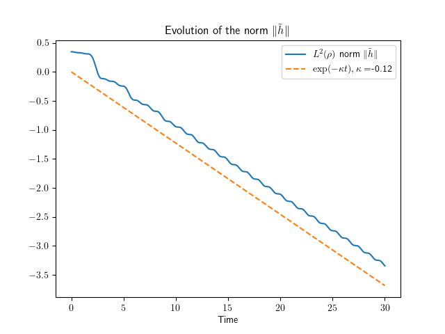
(a) $N=5,\ \ K=20$.

(b) $N=30,\ \ K=20$

Figure 1. Exponential decay of the norm $\|\tilde{h}\|_{L^{2}(\mathscr{M})}$ for different parameter $K$ and $N$ (y-axis in logscale).

6.3. Double well potential

The potential is here $\phi(x)=(x-1)^{2}(x+1)^{2}$. We also normalize $\phi$ in order to have $<1>=<\partial_{x}^{2}\phi>=1$.

6.3.1. Perturbation on $\tilde{C}_{2}$ only

For the first test, we set $\tilde{C}_{2}(0,x)=\tilde{P}_{1}(x)$ and the other modes to $0$. On Figure 2, we represent the evolution of the norm $\|\tilde{h}\|_{L^{2}(\mathscr{M})}$, for different truncation parameters $N$. We also use linear interpolation to approximate the rate $\kappa$. We see that the two graphs are almost identical, and that the rate $\kappa$ does not vary with $N$. This supports the conjecture of the operator norm (see Annex B) indenpendently of the potential.

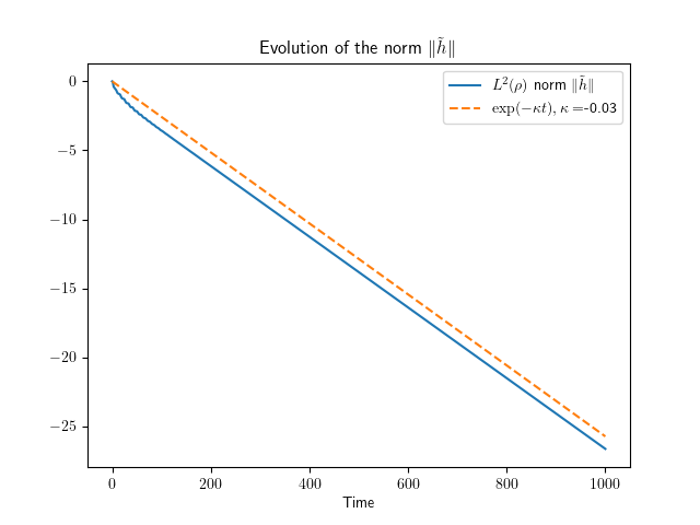
(a) $N=5,\ \ K=20$.

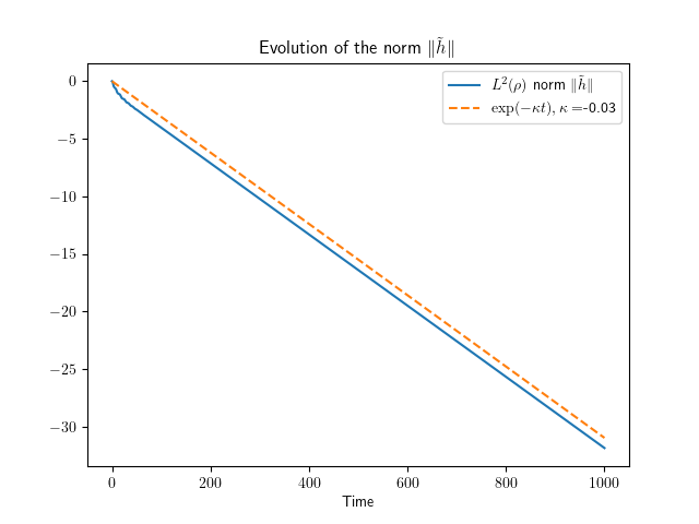
(b) $N=30,\ \ K=20$

Figure 2. Exponential decay of the norm $\|\tilde{h}\|_{L^{2}(\mathscr{M})}$ for different parameter $K$ and $N$ (y-axis in logscale).

6.3.2. Perturbation on $\tilde{C}_{0}$ and $\tilde{C}_{2}$ only

For the second test, we set $\tilde{C}_{0}(0,x)=\tilde{P}_{1}(x)+\tilde{P}_{2}(x)$, $\tilde{C}_{2}(0,x)=-\sqrt{2}<\phi,\tilde{P}_{2}>+\tilde{P}_{1}(x)$ and the other modes to $0$. On Figure 3, we represent the evolution of the pertubation $\tilde{h}$ at different instants. Notice the transfer between the two wells, and the range of values slowly shrinking.

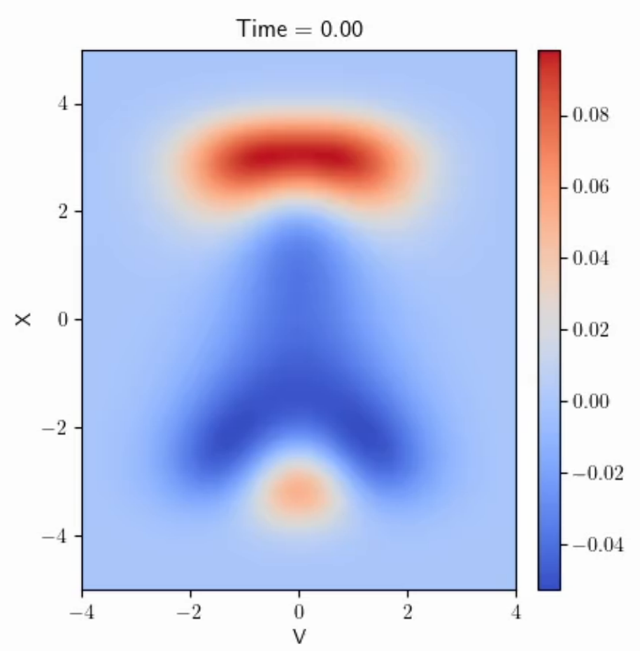
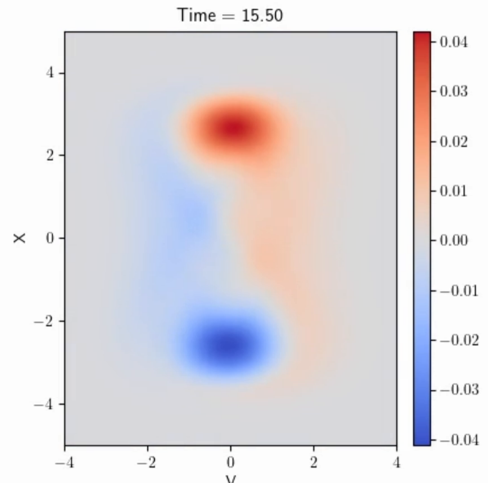
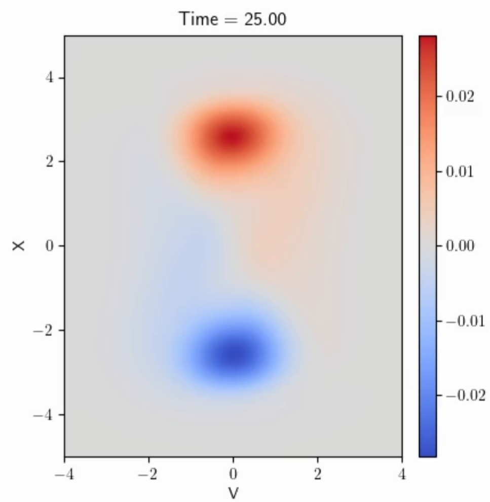
Figure 3. Evolution of the perturbation in the $(x,v)$-plane.

Appendix A Orthonormal polynomials

In this appendix, we gather definitions, notations and important results on the orthonormal polynomials sequences associated with a weight of the form $\rho(x)=e^{-\phi(x)}$. The potential $\phi$ is an even polynomial of degree $2m$, which can be expanded in the canonical basis:

$$\phi(x)=\sum_{i=0}^{m}\gamma_{i}x^{2i}$$

with positive leading coefficient $\gamma_{m}$.

A.1. Exponential weight for general potential

Let $(P_{n})_{n\in\mathbb{N}}$ be the sequence of orthogonal polynomials built by applying the Gram-Schmidt orthogonalization process to the sequence $(x^{n})_{n\in\mathbb{N}}$ with the $L^{2}(\rho)$ scalar product. Now, consider the sequence of polynomials $(\tilde{P}_{n})_{n\in\mathbb{N}}$ defined by the following recurrence relation:

$$\left\{\begin{array}[]{ccc}x\tilde{P}_{n}(x)&=&a_{n+1}\tilde{P}_{n+1}(x)+a_{n}\tilde{P}_{n-1}(x)\ \forall n\geq 1,\\ \tilde{P}_{0}=\dfrac{1}{a_{0}}&\ ;\ \tilde{P}_{-1}=0.&\end{array}\right.$$ (A.1)

The coefficients $(a_{k})_{k\in\mathbb{N}}$ are defined by the formula below (see [6]):

$$a_{0}=\sqrt{\int_{\mathbb{R}}\rho(t)dt};\ \ a_{k}=\sqrt{\dfrac{\int_{\mathbb{R}}P_{k}(t)^{2}\rho(t)dt}{\int_{\mathbb{R}}P_{k-1}(t)^{2}\rho(t)dt}}\ \ ,k\in\mathbb{N}^{*}.$$ (A.2)

The polynomials $(\tilde{P}_{n})_{n\in\mathbb{N}}$ are the orthonormal polynomials of $L^{2}(\rho)$, and they constitute a Hilbert basis of $L^{2}(\rho)$. The two sequences of polynomials are related by the following normalization:

$$\tilde{P}_{k}=\dfrac{P_{k}}{\|P_{k}\|}\ \forall k\in\mathbb{N}.$$

Fix $N\in\mathbb{N}$. Every function of $L^{2}(\rho)$ can be projected on the finite-dimensional space $X_{N}:=Span\{\tilde{P}_{n}\ |\ n=0,1,...,N\}$. The orthogonal projection on $X_{N}$ is noted $\Pi_{X_{N}}$, and

$$\Pi_{X_{N}}f=\sum_{k=0}^{N}\int_{\mathbb{R}}f\tilde{P}_{k}\rho dy\tilde{P}_{k}.$$

An important property is the asymptotic behaviour of the coefficients $a_{n}$, established by Magnus in :

Theorem A.1 ([7], Theorem 6.1).

Let $\phi$ a polynomial of even degree $2m$ and of leading coefficient $\gamma_{m}>0$. Then

$$a_{n}\sim\left(\dfrac{(m-1)!^{2}}{2\gamma_{m}(2m-1)!}n\right)^{1/2m}.$$ (A.3)

A.2. Hermite polynomials

In this part we consider the special case where
$\phi(x)=\frac{1}{2}(x^{2}+\ln(2\pi))$. The orthonormal polynomial sequence $(\tilde{H}_{k})_{k\in\mathbb{N}}$ of $L^{2}(\rho)$ are the so-called Hermite orthonormal polynomials. They are defined by the following recurrence relation:

$$\left\{\begin{array}[]{ccc}v\tilde{H}_{k}(v)&=&\sqrt{k+1}\tilde{H}_{k+1}(v)+\sqrt{k}\tilde{H}_{k-1}(v)\ \ \forall k\geq 1,\\ \tilde{H}_{0}=1&\ ;\ \tilde{H}_{-1}=0.\end{array}\right.$$

They enjoy a richer structure, and satisfy an important differential property:

$$\tilde{H}^{{}^{\prime}}_{k}(v)=\sqrt{k}\tilde{H}_{k-1}(v)\ \forall k\in\mathbb{N}.$$

Appendix B Conjecture and remarks on operators norm

We come back in this appendix on the inequalities (5.5)-(5.8). They define a constant $K_{N}>0$, which possibly depends on $N$. We conjecture that in fact it does not depend on $N$.

Conjecture 1.

There exists a constant $K>0$ independant of $N$ such that:

$$\sup_{f\in X_{N},f\neq 0}\dfrac{\|\Omega^{-1/2}\Pi_{X_{N}}\partial_{x}^{*}f\|}{\|f\|}\leq K,$$ (B.1)

$$\sup_{f\in X_{N},f\neq 0}\dfrac{\|\Omega^{-1}\partial_{x}\Pi_{X_{N}}\partial_{x}^{*}f\|}{\|f\|}\leq K,$$ (B.2)

$$\sup_{f\in X_{N},f\neq 0}\dfrac{\|\Omega^{-1}\Pi_{X_{N}}\partial_{x}^{*}\Pi_{X_{N}}\partial_{x}^{*}f\|}{\|f\|}\leq K,$$ (B.3)

$$\sup_{f\in X_{N},f\neq 0}\dfrac{\|\Omega^{-1}\Pi_{X_{N}}\partial_{x}^{*}\partial_{x}f\|}{\|f\|}\leq K.$$ (B.4)

As established by the previous computations, hypocoercivity constants of the scheme are independent of $N$ if this conjecture is true. We have not succeeded in either disproving or proving the conjecture. Nevertheless, in this appendix, we expose some ideas. We will set the degree of the potential $\phi$ to $2m=4$, so $m=2$. This will enable us to work on a non-Hermite case, while keeping the notations simple.

B.1. Expressions of operators in the polynomial basis $(\tilde{P}_{k})_{k\in\mathbb{N}}$

We can try to write the operators involved in the conjecture in the basis $(\tilde{P}_{k})_{k\in\mathbb{N}}$. We will work with $f\in X_{N}$.

B.1.1. The projection $\Pi_{X_{N}}$:

The projection $\Pi_{X_{N}}$ is defined on $L^{2}(\rho)$, and moreover we have

$$\Pi_{X_{N}}\tilde{P}_{k}=\left\{\begin{array}[]{cc}\tilde{P}_{k}&\mbox{ if }k\leq N,\\ 0&\mbox{ else.}\end{array}\right.$$

B.1.2. The adjoint operators $\partial_{x}$ and $\partial_{x}^{*}$:

Let us start by writing the multiplication operator by $\partial_{x}\phi$ in the basis $(\tilde{P}_{k})_{k\in\mathbb{N}}$. The following result is proved in [3]:

Theorem B.1 (Strong Poincaré inequality).

There exists a constant $C_{p}>0$ such that for all $f\in H^{1}(\rho)$,

$$\int_{\mathbb{R}}(1+\phi^{{}^{\prime}2}(x))|f(x)-<f>|^{2}\rho(x)dx\leq C_{p}\int_{\mathbb{R}}f^{{}^{\prime}2}(x)\rho(x)dx$$

where $<f>:=\int_{\mathbb{R}}f\rho dx$ denotes the mean value of $f$ with respect to the measure $\rho(x)dx$.

We deduce directly that the domain of the multiplication operator by $\partial_{x}\phi$ contains $H^{1}(\rho)$. Since $X_{N}\subset H^{1}(\rho)$, we can now compute the infinite matrix of the operator $\partial_{x}\phi$ in the basis $(\tilde{P}_{k})_{k\in\mathbb{N}}$. Let $f=\sum_{l=0}^{\infty}\hat{f}_{l}\tilde{P}_{l}\in H^{1}(\rho)$. We have

$$\partial_{x}\phi f=\sum_{k=0}^{\infty}\sum_{l=0}^{\infty}<\partial_{x}\phi\tilde{P}_{l},\tilde{P}_{k}>\hat{f}_{l}\tilde{P}_{k}.$$

Thus, if we denote $\Phi$ the infinite symmetric real matrix with coefficients $\Phi_{k,l}=<\partial_{x}\phi\tilde{P}_{l},\tilde{P}_{k}>$, with $k,l\in\mathbb{N}$, then

$$\partial_{x}\phi f=\sum_{k=0}^{\infty}\sum_{l=0}^{\infty}\Phi_{k,l}\hat{f}_{l}\tilde{P}_{k}.$$

Consequently, $\partial_{x}\phi$ is represented in the orthonormal polynomial basis by the matrix $\Phi$. We compute the coefficients $\Phi_{k,l}$.

Since $\Phi$ is symmetrical and $\tilde{P}_{k}\perp\mathbb{R}_{k-1}[X]$, the matrix $\Phi$ is a band matrix with bandwidth 7. The parity of $\phi$ implies that $\tilde{P}_{k}$ has the same parity as $k$. Thus, $\Phi_{k,k-2}=0$ for all $k\geq 0$ as this is the integral of an odd function on $\mathbb{R}$. This leaves 5 diagonals to calculate. We know from [7] that

$$\Phi_{k,k}=0\ ;\ \Phi_{k,k-1}=\dfrac{k}{a_{k}}:=l_{k}.$$

It therefore remains to calculate $\Phi_{k,k-3}$ for $k\geq 3$. From the definition of $\phi$ and by orthogonality, we have that

$$<\partial_{x}\phi\tilde{P}_{k-3},\tilde{P}_{k}>=4\gamma_{2}<x^{3}\tilde{P}_{k-3},\tilde{P}_{k}>.$$

By iterating the recurrence relation (A.1), we can calculate $x^{3}\tilde{P}_{k}$. We then find that

$$\Phi_{k,k-3}=<\partial_{x}\phi\tilde{P}_{k-3},\tilde{P}_{k}>=4\gamma_{2}a_{k}a_{k-1}a_{k-2}:=p_{k-2}.$$

Finally, we can represent the matrix $\Phi$:

$$\Phi=\begin{pmatrix}0&l_{1}&0&p_{1}&0&0&\ddots\\ l_{1}&0&l_{2}&0&p_{2}&0&\ddots\\ 0&l_{2}&0&l_{3}&0&p_{3}&\ddots\\ p_{1}&0&l_{3}&0&l_{4}&0&\ddots\\ 0&p_{2}&0&l_{4}&0&l_{5}&\ddots\\ 0&0&p_{3}&0&l_{5}&0&\ddots\\ \ddots&\ddots&\ddots&\ddots&\ddots&\ddots&\ddots\\ \end{pmatrix}$$

The coefficients have values calculated above, and according to the theorem A.3, $p_{n}\sim n^{3/4}$ and $l_{n}\sim n^{3/4}$.

We can now calculate the matrices representing the operators $\partial_{x}$ and $\partial_{x}^{*}$. Let $f=\sum_{l=0}^{\infty}\hat{f}_{l}\tilde{P}_{l}\in H^{1}(\rho)$. We have

$$\partial_{x}f = \sum_{k=0}^{\infty}<\partial_{x}f,\tilde{P}_{k}>\tilde{P}_{k}$$

$$= \sum_{k=0}^{\infty}<f,\partial_{x}\phi\tilde{P}_{k}-\partial_{x}\tilde{P}_{k}>\tilde{P}_{k}$$

$$= \partial_{x}\phi f-\sum_{k=0}^{\infty}<f,\partial_{x}\tilde{P}_{k}>\tilde{P}_{k}$$

$$= \partial_{x}\phi f-\sum_{k=0}^{\infty}\sum_{l=0}^{k-1}\hat{f}_{l}<\tilde{P}_{l},\partial_{x}\tilde{P}_{k}>\tilde{P}_{k}$$

$$= \partial_{x}\phi f-\sum_{k=0}^{\infty}\sum_{l=0}^{k-1}\hat{f}_{l}<\partial_{x}\phi\tilde{P}_{l},\tilde{P}_{k}>\tilde{P}_{k}.$$

It follows that

$$\partial_{x}^{*}f=\sum_{k=0}^{\infty}\sum_{l=0}^{k-1}\hat{f}_{l}<\partial_{x}\phi\tilde{P}_{l},\tilde{P}_{k}>\tilde{P}_{k}.$$

The matrix representing $\partial_{x}^{*}$ is the lower part of $\Phi$. Similarly, since $\partial_{x}+\partial_{x}^{*}=\partial_{x}\phi$, the matrix representing $\partial_{x}$ is the upper part of $\Phi$.

B.1.3. The operator $\Omega$

It is now easy to write the matrix reprensenting the operator $\Omega=\partial_{x}^{*}\partial_{x}+1$:

$$\begin{pmatrix}1&0&0&0&0&0&\ddots\\ 0&1+l_{0}^{2}&0&l_{0}p_{0}&0&0&\ddots\\ 0&0&1+l_{1}^{2}&0&l_{1}p_{1}&0&\ddots\\ 0&l_{0}p_{0}&0&1+p_{0}^{2}+l_{2}^{2}&0&l_{2}p_{2}&\ddots\\ 0&0&l_{1}p_{1}&0&1+p_{1}^{2}+l_{3}^{2}&0&\ddots\\ 0&0&&l_{2}p_{2}&0&1+p_{2}^{2}+l_{4}^{2}&\ddots\\ \ddots&\ddots&\ddots&\ddots&\ddots&\ddots&\ddots\\ \end{pmatrix}$$

Unfortunately, inverting and taking the square root of this matrix is very difficult, as it is not diagonal as in the Hermite case. Direct calculation of the composition product seems impossible. We may search for a differential operator diagonalized by the basis $(\tilde{P}_{k})_{k\in\mathbb{N}}$. Consider the first inequality conjectured (5.34). To estimate the operator norm of $\Omega^{-1/2}\Pi_{X_{N}}\partial_{x}^{*}$, we can estimate the norm of its adjoint $\partial_{x}\Pi_{X_{N}}\Omega^{-1/2}$. If $A$ and $B$ are two operators, then we define its commutator by $[A,B]:=AB-BA$. Let $f\in X_{N}$.

$$\partial_{x}\Pi_{X_{N}}\Omega^{-1/2}f=\partial_{x}\Omega^{-1/2}f+\partial_{x}[\Pi_{X_{N}},\Omega^{-1/2}]f.$$

From [3], we know that $\|\partial_{x}\Omega^{-1/2}f\|\leq\|f\|$. It therefore remains to estimate the norm of $\partial_{x}[\Pi_{X_{N}},\Omega^{-1/2}]f$. Now,

$$\|[\Pi_{X_{N}},\Omega^{-1/2}]f\|_{H^{1}(\rho)}^{2} = \|\Omega^{1/2}[\Pi_{X_{N}},\Omega^{-1/2}]f\|^{2}$$

$$= \|\Omega^{1/2}\Pi_{X_{N}}\Omega^{-1/2}f-f\|^{2}.$$

Consequently, we find that:

$$\|\partial_{x}[\Pi_{X_{N}},\Omega^{-1/2}]f\|\leq(\|\Omega^{1/2}\|_{H^{1}(\rho)\to L^{2}(\rho)}\|\Pi_{X_{N}}\|_{H^{1}(\rho)\to H^{1}(\rho)}\|\Omega^{-1/2}\|_{L^{2}(\rho)\to H^{1}(\rho)}+1)\|f\|.$$

Since the norms $\|\Omega^{-1/2}\|_{L^{2}(\rho)\to H^{1}(\rho)}$ and $\|\Omega^{1/2}\|_{H^{1}(\rho)\to L^{2}(\rho)}$ are finite, it remains to study the norm of the projection $\|\Pi_{X_{N}}\|_{H^{1}(\rho)\to H^{1}(\rho)}$. Let $f=\sum_{l=0}^{\infty}\hat{f}_{l}\tilde{P}_{l}\in H^{1}(\rho)$. The following notation is introduced:

$$\underline{\hat{f}}_{k}=\left\{\begin{array}[]{cc}\hat{f}_{k}&\mbox{ if }k\leq N,\\ 0&\mbox{ else. }\end{array}\right.$$

Thanks to the matrix expression of $\partial_{x}$, we can calculate the norm $\|\Pi_{X_{N}}f\|_{H^{1}(\rho)}^{2}$

$$\|\Pi_{X_{N}}f\|_{H^{1}(\rho)}^{2} = \|\Pi_{X_{N}}f\|^{2}+\|\partial_{x}\Pi_{X_{N}}f\|^{2}$$

$$\leq \|f\|^{2}+\|\partial_{x}\Pi_{X_{N}}f\|^{2}$$

$$= \|f\|^{2}+\sum_{k=0}^{\infty}(l_{k+1}\underline{\hat{f}}_{k+1}+p_{k+1}\underline{\hat{f}}_{k+3})^{2}$$

$$= \|f\|^{2}+\sum_{k=0}^{N-3}(l_{k+1}\hat{f}_{k+1}+p_{k+1}\hat{f}_{k+3})^{2}+(l_{N-1}\hat{f}_{N-1})^{2}+(l_{N}\hat{f}_{N})^{2}$$

$$\leq \|f\|^{2}+\sum_{k=0}^{\infty}(l_{k+1}\hat{f}_{k+1}+p_{k+1}\hat{f}_{k+3})^{2}+(l_{N-1}\hat{f}_{N-1})^{2}+(l_{N}\hat{f}_{N})^{2}$$

$$\leq \|f\|^{2}+\|\partial_{x}f\|^{2}+(l_{N-1}\hat{f}_{N-1})^{2}+(l_{N}\hat{f}_{N})^{2}$$

$$\leq \|f\|_{H^{1}(\rho)}^{2}+(l_{N-1}\hat{f}_{N-1})^{2}+(l_{N}\hat{f}_{N})^{2}.$$

We then wish to control the residual terms $(l_{N-1}\hat{f}_{N-1})^{2}+(l_{N}\hat{f}_{N})^{2}$ independently of $N$ by the norm $\|f\|_{H^{1}(\rho)}^{2}$. We may look for a regularity theorem on the coefficients of $f$. We will proceed as in the Hermite case and look for a self-adjoint operator diagonalized by the basis $(\tilde{P}_{k})_{k\in\mathbb{N}}$ whose domain would be $H^{1}(\rho)$. Unfortunately, we do not know any no differential equation satisfied by orthonormal polynomials associated with a general exponential weight. We could try to imitate the Hermite case, and use the product $L^{*}L$ where

$$L=\begin{pmatrix}0&0&0&0&0&0&\ddots\\ l_{1}&0&0&0&0&0&\ddots\\ 0&l_{2}&0&0&0&0&\ddots\\ 0&0&l_{3}&0&0&0&\ddots\\ 0&0&0&l_{4}&0&0&\ddots\\ 0&0&0&0&l_{5}&0&\ddots\\ \ddots&\ddots&\ddots&\ddots&\ddots&\ddots&\ddots\\ \end{pmatrix}$$

We have that $L^{*}L$ is diagonal, and its eigenvalues are exactly the real $l_{n}$:

$$L^{*}L=\begin{pmatrix}0&0&0&0&0&0&\ddots\\ 0&l_{1}&0&0&0&0&\ddots\\ 0&0&l_{2}&0&0&0&\ddots\\ 0&0&0&l_{3}&0&0&\ddots\\ 0&0&0&0&l_{4}&0&\ddots\\ 0&0&0&0&0&l_{5}&\ddots\\ \ddots&\ddots&\ddots&\ddots&\ddots&\ddots&\ddots\\ \end{pmatrix}$$

There is no reason why the domain of $L$ would contain $H^{1}(\rho)$, since $L\neq\partial_{x}^{*}$ in the general case. Therefore, no conclusion can be drawn.

References

- [1] Marianne Bessemoulin-Chatard, Maxime Herda, and Thomas Rey. Hypocoercivity and diffusion limit of a finite volume scheme for linear kinetic equations. Mathematics of Computation, 89(323):1093–1133, 2020.
- [2] Alain Blaustein and Francis Filbet. On a discrete framework of hypocoercivity for kinetic equations. Mathematics of Computation, 93(345):163–202, 2024.
- [3] Kleber Carrapatoso, Jean Dolbeault, Frédéric Hérau, Stéphane Mischler, and Clément Mouhot. Weighted Korn and Poincaré-Korn inequalities in the Euclidean space and associated operators. Archive for Rational Mechanics and Analysis, 343(3):1565–1596, 2022.
- [4] Kleber Carrapatoso, Jean Dolbeault, Frédéric Hérau, Stéphane Mischler, Clément Mouhot, and Christian Schmeiser. Special macroscopic modes and hypocoercivity. Journal of the European Mathematical Society, 2023. 65 pages, 1 figure.
- [5] Guillaume Dujardin, Frédéric Hérau, and Pauline Lafitte. Coercivity, hypocoercivity, exponential time decay and simulations for discrete fokker–planck equations. Numerische Mathematik, 144(3):615–697, 2020.
- [6] Walter Gautschi. Orthogonal Polynomials: Computation and Approximation. Oxford University Press, 04 2004.
- [7] A. P. Magnus. On freud’s equations for exponential weights. Journal of Approximation Theory, 46(1):65–99, 1986.
- [8] Alessio Porretta and Enrique Zuazua. Numerical hypocoercivity for the kolmogorov equation. Mathematics of Computation, 86(303):pp. 97–119, 2017.