Emergence of ecological structure and species rarity from fluctuating metabolic strategies

Abstract

Ecosystems often demonstrate the coexistence of numerous species competing for limited resources, with pronounced rarity and abundance patterns. A potential driver of such coexistence is environmental fluctuations that favor different species over time. However, how to include and treat such temporal variability in existing consumer-resource models is still an open problem. In this study, we examine the role of correlated temporal fluctuations in metabolic strategies within a stochastic consumer-resource framework, reflecting change of species behavior in response to the environment. In some conditions, we are able to solve analytically the species abundance distributions, through path integral formalism. Our results reveal that stochastic dynamic metabolic strategies induce community structures that align more closely with empirical ecological observations and contribute to the violation of the Competitive Exclusion Principle (CEP). The degree of CEP violation is maximized under intermediate competition strength, leading to an intermediate competition hypothesis. Furthermore, when non-neutral effects are present, maximal biodiversity is achieved for intermediate values of the amplitude of fluctuations. This work not only challenges traditional ecological paradigms, but also establishes a robust theoretical framework for exploring how temporal dynamics and stochasticity drive biodiversity and community.

I Introduction

Highly biodiverse ecosystems are ubiquitous [1, 2]. Examples include plants, birds, animals, and microorganisms, just to name a few. The astonishing richness of biodiversity is reflected in the fact that around 1.75 million species have been identified; however, this figure represents only about 20% of the estimated total that may exist [3, 2, 4]. Within single trophic levels in the food web, intricate interactions leads to competition among numerous species [5, 6].

The competitive exclusion principle (CEP) [7, 8] asserts that species competing for the same limiting resource cannot stably coexist in equilibrium: one species invariably excludes all others [9]. Mathematically, it is supported by the consumer-resource (CR) model [10] describing the population dynamics of species competing for resources [11, 10, 12, 13]. In stark contrast, Hutchinson’s “paradox of the plankton” defies this prediction, with thousands of plankton species coexisting despite feeding on a common pool of limited resources [14, 15, 16]. Similar observations are evident in microbial ecosystems [17] and terrestrial plant communities [18, 12]. On the other hand, the empirical data reveal that typically most individuals in ecological communities belong to a few species [19, 20], i.e. most of the species composing an ecosystems are rare  [21, 22]. It is thus of paramount interest to uncover the physical mechanisms that promote and sustain such biodiverse ecosystems, while also leading to realistic patterns of community structure [23, 24].

The coexistence of numerous species despite limited resources is often attributed to specific mechanisms such as resource partitioning [25, 26], cross-feeding [27, 28], predation [29], and chaotic population dynamics [30]. In recent years, the classical CR model has been extended to incorporate additional mechanisms, including metabolic trade-offs [31], spatial coarse graining [32, 33], dynamic metabolic adaptation [34], and Liebig’s law of the minimum [30], which states that species growth is determined by the scarcest available resource rather than the total resource pool.

While all these mechanisms are realistic and probably important, a fundamental and relevant factor that is omitted in all such models is environmental variability. In fact, ecosystems are generally influenced by fluctuations of various origins [35]. For example, vital rates of organisms may change significantly over time, due to adaptation dynamics [36, 37], environmental variations [38, 39, 40], and eco-evolutionary processes [41, 42, 43]. These temporal variations do not allow population dynamics to reach equilibrium [44] and create conditions under which species can coexist by exploiting different niches or by experiencing fluctuating selection pressures that prevent any one species from dominating indefinitely [45, 46]. Hutchinson [14] notably proposed that the interplay between environmental and biological time scales could prevent competitive exclusion, suggesting that equilibrium would be avoided, and the CEP violated, when these two time scales are relatively close compared to others. This idea aligns with the intermediate disturbance hypothesis (IDH) [46], which posits that biodiversity is maximized at intermediate levels of disturbance. Aside from external disturbances, fluctuations induced by environmental changes or shifts in resource availability can also disrupt competitive hierarchies, preventing dominant species from excluding others and thereby fostering coexistence [47]. In the presence of non-neutral competition, at low levels of fluctuations, competitive exclusion tends to dominate, reducing species richness, while with large fluctuations, the environment becomes too unstable to support diverse communities. This hypothesis provides a framework for understanding how biodiversity is maintained across a variety of ecosystems and emphasizing the dynamic interplay between competition, resource availability, and environmental stability. Despite these insights, for ecological communities composed of numerous species and resources, a comprehensive understanding of the effects of stochastic fluctuations on species abundance distributions predicted by the CR model is still lacking. Moreover, the theoretical validity of the IDH remains the subject of active discussion [48, 49, 50].

To address these gaps, we introduce stochastic fluctuations in species’ metabolic strategies, representing variation of the expressed metabolic functions due to random environmental changes. Recent studies have explored random Lotka-Volterra [51, 52, 53, 54] and random CR [55, 56] models to examine the effective population densities of large ecological communities. However, in CR models, only time-independent (quenched) stochasticity has been considered. In our framework, by contrast, metabolic strategies—the rates at which consumers uptake resources—are modeled as a random process with temporal fluctuations characterized by exponential autocorrelation.

Using the path integral formalism, we derive an effective consumer-resource dynamics in the limit of infinitely many species and resources. These equations enable us to compute the species abundance distribution (SAD) for general correlation times with minimal approximations, and exactly for vanishing correlation times. Our analysis reveals that: (i) predicted species distributions closely align with empirical observations [24], showing Gamma-like distributions for short correlation times; (ii) the CEP is violated for finite correlation times, with stronger violations for shorter correlation times; (iii) maximal CEP violation occurs when competition strength is intermediate, leading to an intermediate competition hypothesis; (iv) in the presence of non-neutral effects, optimal biodiversity is achieved at intermediate levels of fluctuation amplitude, a result related to – but independent from – the intermediate disturbance hypothesis [46].

II Methods

Our aim is to study the effect of temporal fluctuations of organisms’ feeding rates, i.e., of metabolic strategies, on the community structure of ecosystems. We describe a single trophic level, meaning organisms which interact primarily through the utilization of a common pool of nutrients, e.g., arboreal species in a forest or plankton species in the ocean. More explicitly, we consider a consumer-resource model of $S$ species competing for $R$ biotic and substitutable resources. At time $t$, the population size of species $\sigma=1,2,\dots,S$ is $n_{\sigma}(t)$, and the concentration of resource $i=1,2,\dots,R$ is $c_{i}(t)$. These quantities evolve according to the following equations:

$$\dot{n}_{\sigma} =n_{\sigma}\bigg{[}\sum_{i=1}^{R}\alpha_{\sigma,i}(t)c_{i}-\delta_{\sigma}\bigg{]}+\lambda_{n}\ ,$$ (1a)

$$\ \dot{c}_{i} =\mu_{i}c_{i}\bigg{(}1-\dfrac{c_{i}}{\kappa_{i}}\bigg{)}-c_{i}\sum_{\sigma=1}^{S}n_{\sigma}\alpha_{\sigma,i}(t)+\lambda_{c}\ ,$$ (1b)

$$\alpha_{\sigma,i}(t) =\dfrac{\bar{\alpha}}{S}+\dfrac{\Delta_{\sigma,i}+\Sigma Z_{\sigma,i}(t)}{\sqrt{S}}\ ,$$ (1c)

$$\dot{Z}_{\sigma,i} =-\dfrac{Z_{\sigma,i}}{\tau}+\dfrac{\sqrt{1+2\tau}}{\tau}\xi_{\sigma,i}(t)\ ,$$ (1d)

where $\alpha_{\sigma,i}(t)$ is the metabolic strategy characterizing the rate of consumption of resource $i$ by species $\sigma$ at time $t$, $\delta_{\sigma}$ is the death rate of species $\sigma$, $\mu_{i}$ and $\kappa_{i}$, respectively, are the growth rate and carrying capacity of $i$-th resource. All species share the same baseline level for metabolic strategies, given by $\bar{\alpha}/S$; species-specific variations from that baseline are modeled through $\Delta_{\sigma,i}/\sqrt{S}$, which are quenched independent and identically distributed normal random variables, $\Delta_{\sigma,i}\sim\mathcal{N}\big{(}0,\Delta^{2}\big{)}$. The scaling with $S$ in Eq. (1c) is necessary so that the limit $S\to+\infty$ is well-defined [53, 54]. In Eqs. (1c) and (1d), $\xi_{\sigma,i}(t)$ are independent Gaussian white noises with zero mean and delta-correlated in time: $\langle\xi_{\sigma,i}(t)\xi_{\sigma^{\prime},i^{\prime}}(t^{\prime})\rangle=2\delta_{\sigma,\sigma^{\prime}}\delta_{i,i^{\prime}}\delta(t-t^{\prime})$, such that each $Z_{\sigma,i}$ at stationarity behaves as a colored-noise with zero mean and exponentially-correlated in time:

$$\langle Z_{\sigma,i}(t)~Z_{\sigma^{\prime},i^{\prime}}(t^{\prime})\rangle=\delta_{\sigma,\sigma^{\prime}}\delta_{i,i^{\prime}}\dfrac{1+2\tau}{2\tau}e^{-|t-t^{\prime}|/\tau}\equiv\delta_{\sigma,\sigma^{\prime}}\delta_{i,i^{\prime}}q(|t-t^{\prime}|)\ .$$ (2)

Therefore, each $\alpha_{\sigma,i}$ fluctuates about $\bar{\alpha}/S+\Delta_{\sigma,i}/\sqrt{S}$, on time scales longer than $\tau$ whereas on shorter time scale it behaves like a quenched random variable. In the limits of vanishing and infinite correlation time, the temporal correlation in Eq. (2) behaves as

$$\langle Z_{\sigma,i}(t)~Z_{\sigma^{\prime},i^{\prime}}(t^{\prime})\rangle\to\delta_{\sigma,\sigma^{\prime}}\delta_{i,i^{\prime}}\begin{cases}\delta(t-t^{\prime})&~{\rm as}~\tau\to 0\\ 1&~{\rm as}~\tau\to\infty\end{cases}\ .$$ (3)

Notice that in the $\tau\to\infty$ limit the metabolic strategies becomes quenched, independent and identically distributed Gaussian random variables with average $\bar{\alpha}/N$ and variance $\Delta^{2}+\Sigma^{2}$. In Eq. (1c), the parameter $\Sigma$ regulates the amplitude of colored-noise fluctuations. Further, both consumers and resources can immigrate in the system with constant rates $\lambda_{n}$ and $\lambda_{c}$, respectively, which should be set to zero for isolated systems. We show some examples of solutions of Eq. (1) in Fig. 1, displaying the qualitative differences in trajectories for different values of $\tau$: fluctuations in species abundances become larger, and correspondingly turnover between species slows down.

In what follows, for convenience, we set $\delta_{\sigma}=\delta$, $\mu_{i}=\mu$, and $\kappa_{i}=\kappa$ for all consumers and resources. We regard all quantities as dimensionless. We note that choosing to scale metabolic strategies with $R$ instead of $S$ would produce identical results up to a redefinition of constants: $\bar{\alpha}\to\bar{\alpha}S/R,~\Delta\to\Delta\sqrt{S/R},~\Sigma\to\Sigma\sqrt{S/R}\ .$

In the following sections, we give the effective dynamics for Eq. (1) in the limit of infinite species and resource types, with a finite ratio $\nu\equiv S/R$, which defines the competition strength of the ecosystem. After that, we give expression for the stationary distribution of abundances of both species and resources in the case of no quenched disorder being present; these results allow us to illustrate some key predictions of this model. In particular, in the limit of $\tau\to 0$, we can write down the exact stationary distributions of the process, showing directly their dependence on the model’s parameters. For $\tau>0$, we obtain approximated stationary distributions, which depend on the statistics of the full system. Later, we explore the case of both quenched and annealed disorders, illustrating the effect of their interplay.

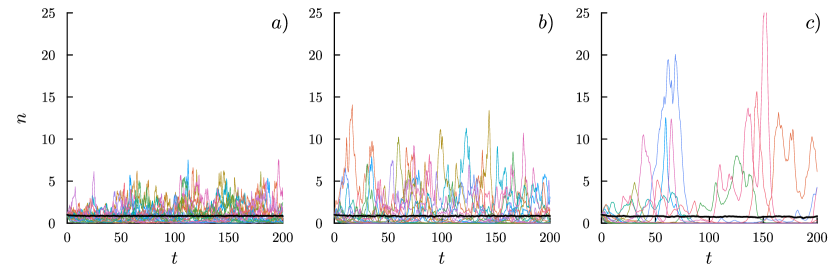
Figure 1: Examples of trajectories of $\{n_{\sigma}\}$, solutions of Eqs. (1), for $\tau=0.1$ (a), $\tau=1$ (b) and $\tau=10$ (c), with all remaining parameters being equal (the values of all other parameters are given in appendix G); in particular, $\Delta=0$. Colored lines show abundances of individual species, of which only 20 are shown for each instance, while the thick black lines represent the average species abundance.

II.1 Effective equations in the thermodynamic limit

Equation (1) describes the dynamics of the population of $S$ species competing for $R$ resources in the presence of stochastic metabolic strategies $\alpha_{\sigma,i}(t)$. While an exact solution of the full model Eq. (1) is not achievable, following Ref. [52, 56] we utilize dynamical mean field theory (DMFT) to derive effective dynamical equations that in some condition we will able to solve analytically. In the limit of infinite numbers of species and resources, with their ratio $\nu$ being fixed and finite, these stochastic differential equations describe the evolutions of the density, $n$, of a representative species and of the concentration of a representative resource, $c$. Both of these differential equations are driven by self-consistent noise, which represents the dynamical effect of all other (infinitely many) species and resources. Here, we report the DMFT equations, while the details of the calculation are relegated to Appendix A. The effective equations read

$$\dot{n} =n\Big{[}\frac{\bar{\alpha}}{\nu}\langle c\rangle-\delta-\frac{1}{\sqrt{\nu}}\xi_{n}+\frac{1}{\nu}\int_{0}^{t}~dt^{\prime}\Big{(}\Delta^{2}+\Sigma^{2}q(|t-t^{\prime}|)\Big{)}G_{c}(t,t^{\prime})n(t^{\prime})+h_{n}\Big{]}+\lambda_{n}\ ,$$ (4a)

$$\dot{c} =\mu c\Big{(}1-\frac{c}{\kappa}\Big{)}-c\Big{[}\bar{\alpha}\langle n\rangle+\xi_{c}+\int_{0}^{t}~dt^{\prime}\Big{(}\Delta^{2}+\Sigma^{2}q(|t-t^{\prime}|)\Big{)}G_{n}(t,t^{\prime})c(t^{\prime})-h_{c}\Big{]}+\lambda_{c}\ ,$$ (4b)

where the noises satisfy the following self-consistent equations:

$$\langle\xi_{n}\rangle =\langle\xi_{c}\rangle=0\ ,$$ (5a)

$$\langle\xi_{n}(t)\xi_{n}(t^{\prime})\rangle =\Big{(}\Delta^{2}+\Sigma^{2}q(|t-t^{\prime}|)\Big{)}\langle c(t)c(t^{\prime})\rangle\ ,$$ (5b)

$$\quad\langle\xi_{c}(t)\xi_{c}(t^{\prime})\rangle =\Big{(}\Delta^{2}+\Sigma^{2}q(|t-t^{\prime}|)\Big{)}\langle n(t)n(t^{\prime})\rangle\ ,$$ (5c)

for two-times correlation function of the driving noise, $q(|t-t^{\prime}|)$, is defined in Eq. (2). Averages denoted by the angular brackets in Eq. (5), are understood to be taken with respect to realizations of the effective dynamics (4). The auxiliary fields, $h_{n}(t)$ and $h_{c}(t)$, have been introduced for mathematical convenience, as they allow us to compute the response functions:

$$G_{n}(t,t^{\prime})=\Bigg{\langle}\frac{\delta n(t)}{\delta h_{n}(t^{\prime})}\Bigg{\rangle}\ ,$$ (6a)

$$G_{c}(t,t^{\prime})=\Bigg{\langle}\frac{\delta c(t)}{\delta h_{c}(t^{\prime})}\Bigg{\rangle}\ .$$ (6b)

Notice that Eqs. (4a) and (4b) are only coupled through the self-consistent conditions (5), which makes the effective equations (4) amenable to analytic calculations.

In the following, we investigate this effective dynamics at steady-state, giving an analytical description in the purely annealed case, i.e., $\Delta=0$, until stated otherwise. Disordered consumer-resources models have been studied with quenched disorder appearing both in metabolic strategies and in resource carrying capacity [56]; in the present work, we focus on disordered metabolic strategies, investigating the role of temporal fluctuations with general autocorrelation time. In this sense, as also mentioned above, our results will recover what found in [56] once we take the limit $\tau\to+\infty$.

II.2 Exact results in the white noise limit

In this section, we solve the Eqs. (4a) and (4b) to obtain the species abundance distribution in the white noise limit: $\tau\to 0$. Specifically, we set the auxiliary fields $h_{n,c}$ equal to 0 and take the limit $\tau\to 0$ (i.e., $q(|t-t^{\prime}|)\to\delta(t-t^{\prime})$), and we obtain the exact steady-state distributions of $n$ and $c$ (see Appendix B for more details):

$$p_{\rm st}^{(n)}(n;\tau=0) \propto n^{-1+d_{n}}e^{-n/b_{n}-\ell_{n}/n}\ ,$$ (7a)

$$p_{\rm st}^{(c)}(c;\tau=0) \propto c^{-1+d_{c}}e^{-c/b_{c}-\ell_{c}/c}\ ,$$ (7b)

where all the constants are defined in Appendix B. Setting the immigration rates $\lambda_{n}=\lambda_{c}=0$ – signifying the system is closed – results in $l_{n}=l_{c}=0$. In this case, the population and resource concentration distributions (7) become Gamma distributions, whereas one obtains truncated Gaussian distributions for the quenched disorder system [56]. Further, this allows us to obtain closed-form expressions for the first two moments of $n$ and $c$. Solving these moments, we can express $\langle n\rangle$ and $\langle c\rangle$ in terms of the models’ parameters, yielding explicit analytical predictions for all steady-state statistics. For $\langle n\rangle$ to be positive (or equivalently for $d_{n}$ to be positive, see Appendix B) the ratio of number of species to the resources has to be smaller than a critical $\nu_{c}$ , i.e., $\nu<\bar{\alpha}\kappa/\delta\equiv\nu_{c}$, failing which all species become extinct.

II.3 Approximate stationary distributions for general correlation time, $\tau$

Generally it is difficult to exactly calculate the stationary-state distributions of processes driven by colored noise. However, for one-dimensional process driven by Gaussian noise with exponential correlation (i.e., an Ornstein-Uhlenbeck process), the uniform colored-noise approximation (UCNA) [57] provides a way to compute the stationary-state distribution. Indeed, the effective variables $n$ and $c$ in Eq. (4) are only coupled through self-consistent conditions  (5), so that the effective dynamics comprises two one-dimensional equations. Furthermore, the correlation functions of both $n$ and $c$ have approximately exponential form, with characteristic times $\tau_{n}$ and $\tau_{c}$ respectively. We apply the UCNA and obtain the approximated stationary distributions of $n$ and $c$ (see Appendix C for calculations):

$$p_{\rm st}^{(n)}(n;\tau) \propto\big{(}n+A_{n}\big{)}n^{-1+\frac{2\tau}{1+2\tau}B_{n}}\exp\bigg{[}\frac{2\tau}{1+2\tau}C_{n}\bigg{(}-\frac{1}{2}n^{2}+D_{n}n\bigg{)}\bigg{]}\ ,$$ (8a)

$$p_{\rm st}^{(c)}(c;\tau) \propto\big{(}c+A_{c}\big{)}c^{-1+\frac{2\tau}{1+2\tau}B_{c}}\exp\bigg{[}\frac{2\tau}{1+2\tau}C_{c}\bigg{(}-\frac{1}{2}c^{2}+D_{c}c\bigg{)}\bigg{]}\ .$$ (8b)

Both distributions in Eq. (8) interpolate between a Gamma and a Gaussian distribution. The various parameters appearing in these distributions, $(A_{x},B_{x},C_{x},D_{x})_{x\in\{n,c\}}$, depend on the first and second moments of $n$ and $c$, as well as their correlation times and all of the models’ parameters, and are reported in Table C1 in Appendix C. Additionally, the UCNA leads to the definition of new constants, on which we comment here briefly. Two of these constants, $\chi_{n}$ and $\chi_{c}$, are related to the memory terms of the effective dynamics (i.e., the integrals in Eq. (4)) through the following simplifying assumption:

$$\int_{0}^{t}G_{x}(t,t^{\prime})q(t,t^{\prime})y(t^{\prime})dt^{\prime}\approx\chi_{x}y(t)\textrm{, for }(x,y)\in\big{\{}(n,c),(c,n)\big{\}}\ .$$ (9)

Moreover, the parameters of the distributions in Eq. (8) depend on two emerging time scales, given by $\bar{\tau}_{x}\equiv(\tau^{-1}+\tau_{x}^{\prime-1})^{-1}$, which is dominated by the smallest between $\tau$ and $\tau^{\prime}_{x}=\tau_{x}\langle x^{2}\rangle/(\langle x^{2}\rangle-\langle x\rangle^{2})$, for $x=n,c$; the origin of these time scales is to be found in the assumption that autocorrelation functions of $n$ and $c$ are exponential, as reported in Appendix C. While moments and correlation times of $n$ and $c$ can be obtained directly from numerical simulations of Eqs. (1), $\chi_{n}$ and $\chi_{c}$ are not directly accessible, and better considered as fitting parameters.

II.4 Evenness as an indicator of effective diversity

As we are working in the limit of infinite number of species and resources (DMFT, Eqs. (4)), it is natural to define fractions of species’ number, with respect to $S$, the maximum number of species in our model ecosystem. We thus want to investigate how populations’ abundances are spread across species. At stationarity, only $S_{*}$ ($\leq S$) species will have non-negligible abundance. If individuals are evenly distributed across all $S$ species then one expects $S_{*}\simeq S$; on the contrary, if the distribution is highly uneven, $S_{*}\ll S$.

A related challenge in both mathematical models and field observations is defining extinction thresholds. In models like ours, species with low fitness exhibit exponentially declining abundances in time, never truly reaching extinction but potentially transitioning between rare and abundant states over time [22]. In field observations, sample size heavily influences the detection of rare species, making it difficult to determine whether a species is locally extinct within a specific sampling framework [58, 59]. To address this, a practical abundance threshold is often applied, but this choice affects observed metrics such as species count. A more robust approach is to weight species abundances based on their magnitudes, avoiding arbitrary thresholds and providing a clearer measure of effective diversity.

These considerations naturally lead to the measure of community evenness [60, 61]. We use evenness to characterize community structure as predicted by our model, Eq. (1), in order to analyze the effect of different mechanisms in shaping ecosystems. Evenness describes community proportions, in the sense of relative rarity of species, clarifying the connection between the SAD and relative abundance distribution (RAD) of an ecosystem  [60, 62, 63].

Given the set of all species abundances in a community, $\{n_{\sigma}\}_{\sigma=1}^{S}$, the relative abundance of consumer species $\sigma$ is

$$p_{\sigma}=\dfrac{n_{\sigma}}{\sum_{\sigma^{\prime}}n_{\sigma^{\prime}}}\ .$$ (10)

Then, we define the evenness of a community in a given state as [64]:

$$D=\dfrac{e^{H}}{S}\ ,$$ (11)

where $H$ is the Shannon entropy:

$$H=-\sum_{\sigma=1}^{S}p_{\sigma}\ln p_{\sigma}\ .$$ (12)

This definition of evenness is particularly suitable for comparing ecosystems with varying numbers of species, while recognizing that evenness and species richness ($S$) represent two distinct yet interconnected dimensions of biodiversity [65]. The evenness metric satisfies $0<D<1$, where $D\approx 0$ indicates communities dominated by a few abundant species, and $D\approx 1$ corresponds to communities where all species have nearly equal abundances.

The metric $D$ can be interpreted as an indicator of the fraction of species, relative to the total $S$, that are most likely to be encountered in a random, uniform sample of the community. This provides insight into the ecosystem’s structure, effectively quantifying the functional fraction of species. In the specific context of a consumer-resource model, where the competition strength is defined as $\nu=S/R$, the product $\nu D$ represents the effective number of species per resource. This metric offers a more precise measure of the violation of the CEP. Furthermore, if $\nu D$ is not monotonic with respect to $\nu$, it implies that the CEP is maximally violated at a specific, non-trivial value of $\nu$.

We have analytically shown that the SAD in the white noise limit is a Gamma distribution (Eqn. (7)). In Appendix D we compute the evenness for this case $n\sim\text{Gamma}\big{(}d,b\big{)}$ in the limit of infinite $S$, and obtain $D=e^{-\psi(1+d)}d$, for the the Digamma function $\psi(z)\equiv\frac{d}{dz}\ln(\Gamma(z))$; see Fig. D1. This shows that $D$ is a well-defined quantity for highly diverse ecosystems, and depends only on one parameter of the SAD.

III Results

We analyzed how fluctuating metabolic strategies shape the structure of consumer-resource ecological communities. These metabolic strategies are characterized by several parameters: the heterogeneity among species ($\Delta$); the amplitude ($\Sigma$) and correlation time ($\tau$) of the fluctuations; and the competition strength ($\nu=S/R$). To study the impact of these parameters on the structure of the community, we employed the evenness ($D$) as a metric that quantifies the balance of abundances of species.

III.1 $\tau=0$

We first considered the case $\Delta=0$, where the long-term interspecific differences in metabolic strategies are negligible compared to temporal fluctuations. By solving the full system, we observed that increasing the correlation time $\tau$ leads to slower but larger fluctuations in species abundances (see Fig. 1). As $\tau\to+\infty$, communities become more uneven, with many rare species and a few abundant ones. This behavior is consistent with the known results for purely quenched disorder [56], where temporal fluctuations are absent.

We studied analytically the case of vanishing correlation time ($\tau\to 0$). We derived a closed-form expression for the species abundance distribution (SAD) (7) and an exact functional form for the evenness (Appendix D). Numerical simulations confirmed the excellent agreement between the theoretical SAD and the empirical distributions obtained from the model (Fig. 2a). This analytical result provides a precise prediction of the SAD for $\tau\to 0$, highlighting that even in the presence of strong fluctuations, the structure of ecological communities remains predictable.

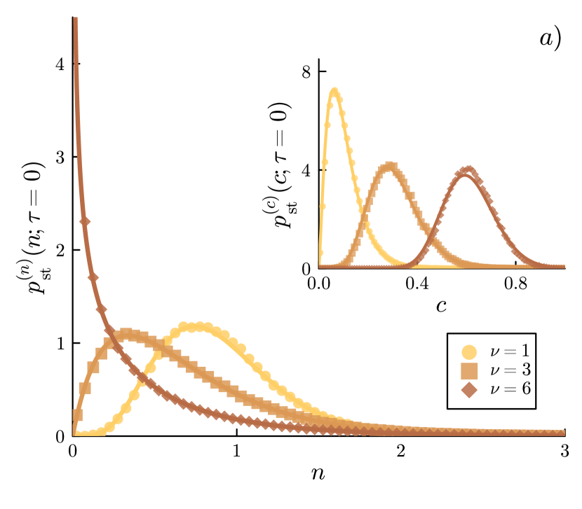
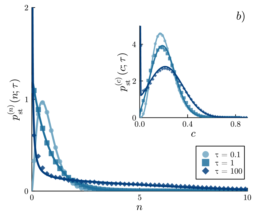
Figure 2: (a) Comparison of empirical stationary distributions (markers), obtained from simulations of Eq. (1), with the corresponding analytical distributions from Eq. (7) (solid lines), for different values of $\nu=S/R$. The analytical results are parameter-free predictions of the DMFT. (b) UCNA prediction for stationary distributions of species and resource abundances for $\nu=2$ with $\tau=0.1$, $1$, and $100$: simulation results (markers) and best-fit of predicted distributions (solid lines). Main panels show the distribution of $n$, while the insets show resource abundances $c$. All parameters used in the simulations are reported in Appendix G.

For larger values of competition strength $\nu$, the SAD peak shifts toward $n=0$, as increasing species diversity for a fixed number of resources leads to lower abundances for most species. Notably, under annealed uncorrelated disorder, the SAD takes the form of a Gamma distribution, consistent with empirical observations from real ecosystems [66, 24, 67]. This result emphasizes the robustness of our model in capturing universal patterns of biodiversity. While our primary focus was on biotic resources, Appendix F demonstrates that similar SADs emerge for abiotic resources, further validating the generality of our findings.

III.2 General $\tau$

For a general $\tau$, a richer phenomenology is observed. Using the Unified Colored Noise Approximation (UCNA), we derived approximate stationary distributions for general $\tau$ (Eq. (8)), which interpolate between Gamma and Gaussian shapes. The parameters of the distributions depend on moments of $n$ and $c$ and their correlation times, which we estimated directly from simulations of the full model, Eq. (1). Having no access to the values of $\chi_{n}$ and $\chi_{c}$ for generic $\tau$, we used these constants as fitting parameters. Fig. 2b shows that the theoretical (approximated) SAD closely matches numerical results.

Similarly to what happens with $\nu$, as $\tau$ increases, the turnover between rare and abundant species slows down (Appendix E). For this reason, rare species will experience longer periods of decay, leading to even lower abundances. In the limit $\tau\to+\infty$, a Gaussian component with large variance emerges in the SAD, representing abundant species, while rare species form a Gamma-like peak near $n=0$. This result is reminiscent of truncated Gaussian distributions observed in quenched-noise models [54, 56]. This is also consistent with the predictions of our model in the limit of long correlation time $\tau\to\infty$.

III.3 CEP violation

A key finding of our work is that temporal fluctuations in metabolic strategies allow the violation the CEP. This violation is quantitatively captured by the metric $\nu D$ (Appendix D), which represents the effective number of coexisting species per resource. Values of $\nu D>1$ indicate that more species coexist than allowed under strict competitive exclusion. For $\tau\to 0$, the relationship between $\nu$ and $D$ is obtained analytically. The violation of the CEP holds robustly across a wide range of model parameters (Fig. 3a).

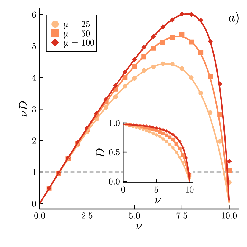
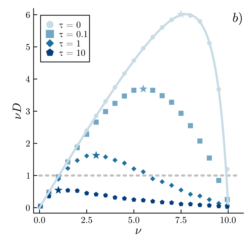
Figure 3: (a) Evenness ($D$) in the white noise limit: $D$ (inset) and $\nu D$ (main panel) as functions of $\nu$ for different values of $\mu$. Markers: numerical simulations. Solid lines: analytical results. (b) $\nu D$ as a function of $\nu$ for different $\tau$ values, with $\mu=100$. Solid line: exact evenness for $\tau=0$. Markers: numerical simulations. Stars indicate maximal $\nu D$ for each $\tau$ among the values found numerically. CEP is violated when $\nu D>1$, a threshold indicated by gray dashed lines. All other parameters used in the simulations are reported in Appendix G.

Interestingly, for moderate values of $\tau$, the violation of the CEP is maximized at an intermediate competition strength (Fig. 3b). In other words, the diversity supported by each resource is higher for intermediate levels of competition, which we refer to as intermediate competition principle, a result only emerging for time-dependent interactions. This result complements the intermediate disturbance principle by considering endogenous ecological forces, as in our model fluctuations in species interactions can lead to effective environmental fluctuations. For $\tau>0$, competitive exclusion can still be overcome, but as $\tau$ increases the optimal value of $\nu D$ decreases, eventually becoming smaller than $1$, and the optimal $\nu$ moves closer to $1$. This aligns with previous results showing that purely quenched disorder does not break the CEP [56]. In all cases, all species go extinct if $\nu\geq\nu_{c}$; correspondingly, $\nu D\to 0$ as $\nu\to\nu_{c}$.

III.4 Combined annealed and quenched disorder

We also investigated the case where both annealed and quenched disorder are present ($\Delta,\Sigma>0$). Fig. 4a shows how the SAD transitions from a Gamma distribution ($\Delta=0$) to a truncated Gaussian as $\Delta\to\Sigma$. Additionally, evenness as a function of $\Sigma$ and $\tau$ (Fig. 4b) reveals a non-trivial region of maximal diversity for $0<\Delta\ll\Sigma$, a result analogous to the intermediate disturbance hypothesis for the case of endogenous fluctuations. This phenomenon does not occur in the purely annealed case; see Fig. E2.

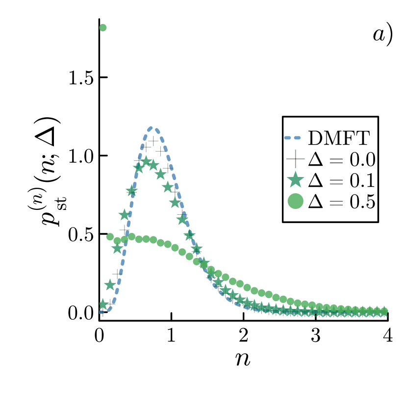
Figure 4: (a) SAD in the case of both quenched and annealed disorder ($\Delta,\Sigma>0$). Comparison between DMFT result in the white noise limit and $\Delta=0$ (dashed line) and empirical SADs with $\tau=0.1$, $\Sigma=1$ and different values of $\Delta$ (markers). We highlight the presence of a highly populated bin of low abundances for $\Delta=0.5$ (marker in the top left corner of the panel). (b) Evenness as function of $\Sigma$ and $\tau$, for $\Delta=0.1$. Fig. E2 in Appendix E is obtained with identical parameters, save for $\Delta$, which is set to zero. Brighter hues denote more even communities. Each point is obtained by computing the stationary evenness of a single realization of the microscopic dynamics, Eqs. (1). Grey dashed lines in panel (b) contour the region of optimal evenness. All other parameters used in the simulations are reported in Appendix G.

IV Discussion and Conclusions

The question of which mechanisms prevent competitive exclusion of species, and how these mechanisms affect ecosystem structure, is a long-standing and important one. Specific biological mechanisms exist that promote coexistence, such as resource partitioning, cross-feeding, and predation. However, real ecosystems are subject to temporal variations in vital rates due to environmental changes and other factors. To capture this dynamic aspect, we studied a consumer-resource model where metabolic strategies are modeled as colored noise, fluctuating around a fixed value with finite correlation time. This approach describes a phenomenon independent of the specific biological details of organisms, allowing predictions to apply to a broad variety of ecosystems.

Assuming that metabolic strategies of different species share the same baseline value, meaning that long-term differences are negligible compared to temporal fluctuations, we derived analytical expressions for the stationary distributions of abundances. In a range of moderate correlation times, the competitive exclusion principle is violated, and the effective number of species per resource is maximized at an intermediate value of competition strength ($\nu=S/R$). Further, our model aligns with empirical observations that species abundance distributions (SADs) in most ecosystems follow a robust pattern of many rare species and few common ones, often approximated by Gamma-like distributions [66, 24, 67]. Non-zero correlation times introduce a Gaussian component to the SAD, which becomes dominant as $\tau$ approaches infinity, consistent with previous findings [56]. While pure Gaussian SADs lack empirical support, moderate correlation times yield distributions where the Gaussian component remains subordinate, resulting in realistic SADs.

Temporal correlations in fluctuations slow the turnover between rare and abundant species, while stronger competition amplifies the impact of each species on others. These combined effects cause SADs to concentrate around rare species, a key characteristic of empirically observed SADs. Our model further predicts that in the white noise limit, all species go extinct when competition strength exceeds a threshold determined by a combination of biological and environmental factors, including baseline metabolic strategies, death rates, and resource carrying capacities. This ecological “hard limit” persists even for finite correlation times.

Non-neutral effects, such as niche availability and overlap, play a significant role in shaping community structure. In our generalized model, species-dependent baseline metabolic strategies reveals that fluctuations of suitable magnitude and correlation time enhance community evenness, reducing the impact of trait differences. These findings provide quantitative support for the intermediate disturbance hypothesis (IDH) in a very broad sense, encompassing temporal variations of diverse origins. Moreover, our results clarify how different aspects of these variations – namely, their magnitude and temporal correlation – interact to define what makes them “intermediate,” an aspect often overlooked in prior work (see e.g., Fig. 1 of Ref. [46]). Our analysis highlights a novel perspective: the emergence of maximal diversity at intermediate competition strength. This result demonstrates that an optimal degree of resource competition can foster coexistence by balancing the effects of competitive exclusion and community evenness. These findings are loosely related to IDH, but offer a quantitative framework to explore its implications in a broader context. By linking competition intensity and temporal fluctuations, our results open new avenues for understanding how ecosystems maintain biodiversity under varying environmental pressures.

Future studies could extend this framework to include non-substitutable resources or metabolic strategies constrained by realistic trade-offs. Analytical derivations for scenarios combining annealed and quenched disorder would further clarify the conditions under which maximal biodiversity regimes emerge. These developments will help refine our understanding of biodiversity patterns across ecosystems and provide a robust theoretical foundation for ecological management and conservation strategies.

Appendix A Derivation of the effective dynamics

In this Appendix we compute the effective equations for the microscopic consumer-resource model, Eqs. (1), which we repeat here:

$$\dfrac{\dot{n}_{\sigma}}{n_{\sigma}} =\sum_{i=1}^{R}\alpha_{\sigma,i}(t)~c_{i}-\delta+h_{\sigma}\,$$ (13)

$$\dfrac{\dot{c}_{i}}{c_{i}} =\mu(1-c_{i}/\kappa)-\sum_{\sigma=1}^{S}\alpha_{\sigma,i}(t)~n_{\sigma}+h_{i},$$ (14)

$$\alpha_{\sigma,i}(t) =\dfrac{\bar{\alpha}}{S}+\dfrac{\Sigma}{\sqrt{S}}Z_{\sigma,i}(t)\ ,$$ (15)

$$\dot{Z}_{\sigma,i} =-\dfrac{Z_{\sigma,i}}{\tau}+\dfrac{\sqrt{1+2\tau}}{\tau}\xi_{\sigma,i}(t)\ .~$$ (16)

Here $\sigma\in\{1,2,\dots,S\}$, $i\in\{1,2,\dots,R\}$. To make calculations less cumbersome, we neglect immigration terms; this is a matter of convenience, and they can be safely reinserted at the end of the derivation. Similarly, in this derivation, we omit the quenched disorder. In fact, the annealed and quenched disorders are integrated out independently, but give rise to analogous terms; thus, the effective equations (4) are recovered from the end results of this calculation simply by performing the substitution $\Sigma^{2}q(|t-t^{\prime}|)\to\Delta^{2}+\Sigma^{2}q(|t-t^{\prime}|)$. Finally, the auxiliary fields $h_{\sigma}$ and $h_{i}$ have been introduced to later compute response functions.

We will calculate the dynamical moment generating function as

$$\mathcal{Z}[\psi,\phi]\equiv\overline{\bigg{\langle}e^{i\sum_{\sigma}\int~dt~\psi_{\sigma}(t)n_{\sigma}(t)+i\sum_{j}\int~dt~\phi_{j}(t)c_{j}(t)}\bigg{\rangle}},$$ (18)

where the angular brackets indicate the average over paths which are solutions of Eqs. (13) and (14) for a given realization of $\alpha_{\sigma,i}(t)$, and the overhead bar stands for the average over ensemble of realizations of $\alpha_{\sigma,i}(t)$; $\mathcal{Z}[0,0]=1$ by normalization of the path’s probability. $\alpha_{\sigma,i}(t)$, whose dynamics is given by Eqs. (15) and (16), is distributed at stationarity according to Gaussian distribution with mean $\frac{\bar{\alpha}}{S}$ and variance $\frac{1}{S}\Sigma^{2}\frac{1+2\tau}{2\tau}$. It also has finite-time exponential correlation, since

$$\langle Z_{\sigma,i}(t)Z_{\sigma^{\prime},i^{\prime}}(t^{\prime})\rangle=\underbrace{\dfrac{1+2\tau}{2\tau}e^{-|t-t^{\prime}|/\tau}}_{q(|t-t^{\prime}|)}\delta_{\sigma,\sigma^{\prime}}\delta_{i,i^{\prime}}\ .$$ (19)

The average over paths in Eq. (18) is written as

$$\langle(\cdots)\rangle =\int\mathcal{D}[n]\mathcal{D}[c]~e^{i\sum_{\sigma}\int~dt~\psi_{\sigma}(t)n_{\sigma}(t)+i\sum_{j}\int~dt~\phi_{j}(t)c_{j}(t)}\prod_{\sigma,t}\delta\bigg{(}\dfrac{\dot{n}_{\sigma}(t)}{n_{\sigma}(t)}-\sum_{j}\alpha_{\sigma,j}(t)c_{j}(t)+\delta-h_{\sigma}(t)\bigg{)}$$

$$\times\prod_{j,t}\delta\bigg{(}\dfrac{\dot{c}_{j}(t)}{c_{j}(t)}-\mu[1-c_{j}(t)/\kappa]+\sum_{\sigma}\alpha_{\sigma,j}(t)n_{\sigma}(t)-h_{j}(t)\bigg{)},$$ (20)

where the $\prod_{\sigma,t}$ indicates the product of over all $\sigma$ indices and over all times $t$. We use the integral representation of the Dirac Delta function,

$$\delta(y-y_{0})\propto\int e^{i\hat{y}(y-y_{0})}d\hat{y}\ ,$$ (21)

in Eq. (20), leading to the following rewriting:

$$\langle(\cdots)\rangle =\int\mathcal{D}[n,\hat{n}]\mathcal{D}[c,\hat{c}]~\exp\bigg{[}i\sum_{\sigma}\int~dt~\psi_{\sigma}(t)n_{\sigma}(t)+i\sum_{j}\int~dt~\phi_{j}(t)c_{j}(t)\bigg{]}$$

$$\times\exp\bigg{[}i\sum_{\sigma}\int~dt~\hat{n}_{\sigma}(t)\bigg{(}\dfrac{\dot{n}_{\sigma}(t)}{n_{\sigma}(t)}-\sum_{j}\alpha_{\sigma,j}(t)c_{j}(t)+\delta-h_{\sigma}(t)\bigg{)}\bigg{]}$$

$$\times\exp\bigg{[}i\sum_{j}\int~dt~\hat{c}_{j}(t)\bigg{(}\dfrac{\dot{c}_{j}(t)}{c_{j}(t)}-\mu[1-c_{j}(t)/\kappa]+\sum_{\sigma}\alpha_{\sigma,j}(t)n_{\sigma}(t)-h_{j}(t)\bigg{)}\bigg{]}$$ (22)

$$=\int\mathcal{D}[n,\hat{n}]\mathcal{D}[c,\hat{c}]~\exp\bigg{[}i\sum_{\sigma}\int~dt~\psi_{\sigma}(t)n_{\sigma}(t)+i\sum_{j}\int~dt~\phi_{j}(t)c_{j}(t)\bigg{]}$$

$$\times\exp\bigg{[}i\sum_{\sigma}\int~dt~\hat{n}_{\sigma}(t)\bigg{(}\dfrac{\dot{n}_{\sigma}(t)}{n_{\sigma}(t)}+\delta-h_{\sigma}(t)\bigg{)}\bigg{]}$$

$$\times\exp\bigg{[}i\sum_{j}\int~dt~\hat{c}_{j}(t)\bigg{(}\dfrac{\dot{c}_{j}(t)}{c_{j}(t)}-\mu[1-c_{j}(t)/\kappa]-h_{j}(t)\bigg{)}\bigg{]}$$ (23)

$$\times\exp\bigg{[}-i\sum_{\sigma}\int~dt~\hat{n}_{\sigma}(t)\sum_{j}\alpha_{\sigma,j}(t)c_{j}(t)\bigg{]}\exp\bigg{[}i\sum_{j}\int~dt~\hat{c}_{j}(t)\sum_{\sigma}\alpha_{\sigma,j}(t)n_{\sigma}(t)\bigg{]}\ ,$$ (24)

where in the last line we have isolated all terms which contain $\alpha_{\sigma,i}(t)$. From the previous expression, we take the average over realizations of $\alpha_{\sigma,i}(t)$:

$$\mathcal{Z}[\psi,\phi]\equiv\overline{\langle(\cdots)\rangle} =\int\mathcal{D}[n,\hat{n}]\mathcal{D}[c,\hat{c}]~\underbrace{\exp\bigg{[}i\sum_{\sigma}\int~dt~\psi_{\sigma}(t)n_{\sigma}(t)+i\sum_{\sigma}\int~dt~\hat{n}_{\sigma}(t)\bigg{(}\dfrac{\dot{n}_{\sigma}(t)}{n_{\sigma}(t)}+\delta-h_{\sigma}(t)\bigg{)}\bigg{]}}_{A[n,\hat{n}]}$$

$$\times\underbrace{\exp\bigg{[}i\sum_{j}\int~dt~\phi_{j}(t)c_{j}(t)+i\sum_{j}\int~dt~\hat{c}_{j}(t)\bigg{(}\dfrac{\dot{c}_{j}(t)}{c_{j}(t)}-\mu[1-c_{j}(t)/\kappa]-h_{j}(t)\bigg{)}\bigg{]}}_{B[n,\hat{n}]}$$

$$\times\underbrace{\overline{\exp\bigg{[}-i\sum_{\sigma,j}\int~dt~\hat{n}_{\sigma}(t)\alpha_{\sigma,j}(t)c_{j}(t)\bigg{]}~~\exp\bigg{[}i\sum_{\sigma,j}\int~dt~\hat{c}_{j}(t)\alpha_{\sigma,j}(t)n_{\sigma}(t)\bigg{]}}}_{\Delta[n,\hat{n},c,\hat{c}]}\ .$$ (25)

Let us rewrite the last term as follows:

$$\Delta[n,\hat{n},c,\hat{c}] =\overline{\exp\bigg{[}i\sum_{\sigma,j}\int~dt~[\hat{c}_{j}(t)n_{\sigma}(t)-\hat{n}_{\sigma}(t)c_{j}(t)]\alpha_{\sigma,j}(t)\bigg{]}}$$

$$=\exp\bigg{[}i\frac{\bar{\alpha}}{S}\sum_{\sigma,j}\int dt[\hat{c}_{j}(t)n_{\sigma}(t)-\hat{n}_{\sigma}(t)c_{j}(t)]\bigg{]}$$

$$\times\exp\bigg{[}-\frac{\Sigma^{2}}{2S}\sum_{\sigma,j}\int dt\int dt^{\prime}[\hat{c}_{j}(t)n_{\sigma}(t)-\hat{n}_{\sigma}(t)c_{j}(t)][\hat{c}_{j}(t^{\prime})n_{\sigma}(t^{\prime})-\hat{n}_{\sigma}(t^{\prime})c_{j}(t^{\prime})]q(|t-t^{\prime}|)\bigg{]}\ ,$$ (26)

where in the last line we used the following result (see Appendix A.1):

$$\overline{\exp\bigg{[}\frac{i\Sigma}{\sqrt{S}}\int_{0}^{t}dt~A(t)Z(t)\bigg{]}}=\exp\bigg{[}-\dfrac{\Sigma^{2}}{2S}\int_{0}^{t}dt_{1}\int_{0}^{t}dt_{2}~A(t_{1})A(t_{2})q(|t_{1}-t_{2}|)\bigg{]}\ .$$ (27)

Thus,

$$\Delta[n,\hat{n},r,\hat{c}] =\exp\bigg{[}i\bar{\alpha}S\int~dt~[\rho_{n}(t)\lambda_{c}(t)-\rho_{c}(t)\lambda_{n}(t)]\bigg{]}$$

$$\times\exp\bigg{[}-\frac{\Sigma^{2}S}{2}\int~dt~\int~dt^{\prime}\big{[}Q_{n}(t,t^{\prime})L_{c}(t,t^{\prime})+Q_{c}(t,t^{\prime})L_{n}(t,t^{\prime})-2K_{n}(t,t^{\prime})K_{c}(t,t^{\prime})\big{]}q(|t-t^{\prime}|)\bigg{]}\ .$$ (28)

In Eq. (A) we defined the following order parameters:

$$\rho_{n}(t)=\dfrac{1}{S}\sum_{\sigma}n_{\sigma}(t) \qquad\qquad\lambda_{n}(t)=\dfrac{1}{S}\sum_{\sigma}\hat{n}_{\sigma}(t)$$ (29)

$$\rho_{c}(t)=\dfrac{1}{S}\sum_{i}c_{i}(t) \qquad\qquad\lambda_{c}(t)=\dfrac{1}{S}\sum_{i}\hat{c}_{i}(t)$$ (30)

$$Q_{n}(t,t^{\prime})=\dfrac{1}{S}\sum_{\sigma}n_{\sigma}(t)n_{\sigma}(t^{\prime}) \qquad\qquad L_{n}(t,t^{\prime})=\dfrac{1}{S}\sum_{\sigma}\hat{n}_{\sigma}(t)\hat{n}_{\sigma}(t^{\prime})$$ (31)

$$Q_{c}(t,t^{\prime})=\dfrac{1}{S}\sum_{i}c_{i}(t)c_{i}(t^{\prime}) \qquad\qquad L_{c}(t,t^{\prime})=\dfrac{1}{S}\sum_{i}\hat{c}_{i}(t)\hat{c}_{i}(t^{\prime})$$ (32)

$$K_{n}(t,t^{\prime})=\dfrac{1}{S}\sum_{\sigma}\hat{n}_{\sigma}(t)n_{\sigma}(t^{\prime}) \qquad\qquad K_{c}(t,t^{\prime})=\dfrac{1}{S}\sum_{i}\hat{c}_{i}(t)c_{i}(t^{\prime})$$ (33)

We use the Dirac Delta function integral representation to treat these order parameters as independent fields: as an example, for $\rho_{n}$ this amounts to inserting into $\mathcal{Z}$ the identity decomposition

$$1=\prod_{t}\delta\bigg{(}\rho_{n}S-\sum_{\sigma}n_{\sigma}(t)\bigg{)}\propto\int~\mathcal{D}[\hat{\rho}]e^{iS\int~dt~\hat{\rho}_{n}(t)\rho_{n}(t)}e^{-i\sum_{\sigma}\int~dt~\hat{\rho}_{n}(t)~n_{\sigma}(t)}$$ (34)

Defining $\Pi=(\rho,\lambda,Q,L,K)$ and $\hat{\Pi}=(\hat{\rho},\hat{\lambda},\hat{Q},\hat{L},\hat{K})$, we finally write $Z$:

$$\mathcal{Z}[\psi,\phi] =\int~\mathcal{D}[\Pi,\hat{\Pi}]~e^{S(\Psi[\Pi,\hat{\Pi}]+\Phi[\Pi])}$$

$$\times\int~\mathcal{D}[n,\hat{n}]\mathcal{A}[n,\hat{n}]~e^{-i\sum_{\sigma}\int~dt[\hat{\rho}_{n}(t)n_{\sigma}(t)+\hat{\lambda}_{n}(t)\hat{n}_{\sigma}(t)]}e^{-i\sum_{\sigma}\int~dt\int~dt^{\prime}~[\hat{Q}_{n}n_{\sigma}n_{\sigma}^{\prime}+\hat{L}_{n}\hat{n}_{\sigma}\hat{n}_{\sigma}^{\prime}+\hat{K}_{n}\hat{n}_{\sigma}n_{\sigma}^{\prime}]}$$

$$\times\int~\mathcal{D}[c,\hat{c}]\mathcal{B}[c,\hat{c}]e^{-i\sum_{j}\int~dt[\hat{\rho}_{c}(t)c_{j}(t)+\hat{\lambda}_{r}(t)\hat{c}_{j}(t)]}e^{-i\sum_{j}\int~dt\int~dt^{\prime}~[\hat{Q}_{c}c_{j}c_{j}^{\prime}+\hat{L}_{c}\hat{c}_{j}\hat{c}_{j}^{\prime}+\hat{K}_{c}\hat{c}_{j}c_{j}^{\prime}]}$$ (35)

where

$$\Psi[\Pi,\hat{\Pi}] =i\int~dt~\big{[}\hat{\rho}_{n}(t)\rho_{n}(t)+\hat{\lambda}_{n}(t)\lambda_{n}(t)+\hat{\rho}_{c}(t)\rho_{c}(t)+\hat{\lambda}_{r}(t)\lambda_{c}(t)\big{]}$$

$$+i\int~dt\int~dt^{\prime}~[\hat{Q}_{n}~Q_{n}+\hat{L}_{n}~L_{n}+\hat{Q}_{c}~Q_{c}+\hat{L}_{c}~L_{c}+\hat{K}_{n}~K_{n}+\hat{K}_{c}~K_{c}](t,t^{\prime})$$ (36)

$$\Phi[\Pi] =i\bar{\alpha}\int~dt~[\rho_{n}(t)\lambda_{c}(t)-\rho_{c}(t)\lambda_{n}(t)]$$

$$-\frac{\Sigma^{2}}{2}\int~dt~\int~dt^{\prime}\big{[}Q_{n}(t,t^{\prime})L_{c}(t,t^{\prime})+Q_{c}(t,t^{\prime})L_{n}(t,t^{\prime})-2K_{n}(t,t^{\prime})K_{c}(t,t^{\prime})\big{]}q(|t-t^{\prime}|)$$ (37)

Now $\mathcal{Z}$ can be written in a compact form:

$$\mathcal{Z}[\psi,\phi] =\int~\mathcal{D}[\Pi,\hat{\Pi}]~e^{S(\Psi[\Pi,\hat{\Pi}]+\Phi[\Pi]+\Omega_{n}[\hat{\Pi}]+\Omega_{c}[\hat{\Pi}])}\ .$$ (38)

To identify $\Omega_{n}[\hat{\Pi}]$, we start from the second line of Eq. (A). We first write $e^{\sum_{\sigma}(\dots)}=\prod_{\sigma}e^{(\dots)}$, and then we factorize the path integral over the $\sigma$ indices, since these integrals are not coupled and can be carried out independently. Finally, we turn the product into a summation through the logarithm function. Since each term inside the summation is identical, the prefactor $1/S$ cancels out, we suppress indices $\sigma$ and define a unique auxiliary fields $h_{n}(t)$, obtaining (we omit some function arguments for ease of notation, using shorthands such as $n(t)n(t^{\prime})\to nn^{\prime}$)

$$\Omega_{n}[\hat{\Pi}] =\ln\int~\mathcal{D}[n,\hat{n}]\exp\bigg{[}i\int~dt~\psi(t)n(t)+i\int~dt~\hat{n}(t)\bigg{(}\dfrac{\dot{n}(t)}{n(t)}+\delta-h_{n}(t)\bigg{)}\bigg{]}$$

$$\times\exp\bigg{[}-i\int~dt[\hat{\rho}_{n}(t)n(t)+\hat{\lambda}_{n}(t)\hat{n}(t)]-i\int~dt\int~dt^{\prime}~[\hat{Q}_{n}nn^{\prime}+\hat{L}_{n}\hat{n}\hat{n}^{\prime}+\hat{K}_{n}\hat{n}n^{\prime}]\bigg{]}\ .$$ (39)

In a similar manner we obtain the following object:

$$\Omega_{c}[\hat{\Pi}] =\dfrac{1}{\nu}\ln\int~\mathcal{D}[c,\hat{c}]\exp\bigg{[}i\int~dt~\phi(t)c(t)+i\int~dt~\hat{c}(t)\bigg{(}\dfrac{\dot{c}(t)}{c(t)}-\mu[1-c(t)/\kappa]-h_{c}(t)\bigg{)}\bigg{]}$$

$$\times\exp\bigg{[}-i\int~dt[\hat{\rho}_{c}(t)c(t)+\hat{\lambda}_{r}(t)\hat{c}(t)]-i\int~dt\int~dt^{\prime}~[\hat{Q}_{c}cc^{\prime}+\hat{L}_{c}\hat{c}\hat{c}^{\prime}+\hat{K}_{c}\hat{c}c^{\prime}]\bigg{]}$$ (40)

Here, $\nu=S/R$ appears as sums over the $i$ indices give $R$ identical contributions.

$\mathcal{Z}$, as given in Eqs. (38), can be approximated using the saddle-point method for large $S$ and $R$, with fixed $\nu$:

$$\mathcal{Z}\approx e^{S(\Psi[\Pi^{*},\hat{\Pi^{*}}]+\Phi[\Pi^{*}]+\Omega_{n}[\hat{\Pi^{*}}]+\Omega_{c}[\hat{\Pi^{*}}])},$$ (41)

where the fields marked by $*$ solve the saddle point equations:

$$\dfrac{\delta\Psi}{\delta\Pi}+\dfrac{\delta\Phi}{\delta\Pi}=0\ ,$$ (42)

$$\dfrac{\delta\Psi}{\delta\hat{\Pi}}+\dfrac{\delta\Omega_{n}}{\delta\hat{\Pi}}+\dfrac{\delta\Omega_{c}}{\delta\hat{\Pi}}=0\ .~$$ (43)

Eq. (42) is solved by

$$\hat{\rho}_{n}(t)=-\bar{\alpha}\lambda_{c}(t)=0 \qquad\qquad\hat{\lambda}_{n}(t)=\bar{\alpha}\rho_{c}(t)$$ (44)

$$\hat{\rho}_{c}(t)=\bar{\alpha}\lambda_{n}(t)=0 \hat{\lambda}_{r}(t)=-\bar{\alpha}\rho_{n}(t)$$ (45)

$$i\hat{Q}_{n}=\frac{\Sigma^{2}}{2}L_{c}~q(|t-t^{\prime}|)=0 i\hat{L}_{n}=\frac{\Sigma^{2}}{2}Q_{c}q(|t-t^{\prime}|)$$ (46)

$$i\hat{Q}_{c}=\frac{\Sigma^{2}}{2}L_{n}~q(|t-t^{\prime}|)=0 i\hat{L}_{c}=\frac{\Sigma^{2}}{2}Q_{n}q(|t-t^{\prime}|)$$ (47)

$$i\hat{K}_{n}=-\Sigma^{2}K_{c}~q(|t-t^{\prime}|) i\hat{K}_{c}=-\Sigma^{2}K_{n}q(|t-t^{\prime}|)$$ (48)

Eq. (43) instead gives

$$\rho_{n}(t)=\langle n\rangle_{\Omega_{n}} \qquad\qquad\lambda_{n}(t)=\langle\hat{n}\rangle_{\Omega_{n}}$$ (49)

$$\rho_{c}(t)=\dfrac{1}{\nu}\langle c\rangle_{\Omega_{c}} \lambda_{c}(t)=\dfrac{1}{\nu}\langle\hat{c}\rangle_{\Omega_{c}}$$ (50)

$$Q_{n}=\langle nn^{\prime}\rangle_{\Omega_{n}} L_{n}=\langle\hat{n}\hat{n}^{\prime}\rangle_{\Omega_{n}}$$ (51)

$$K_{n}=\langle\hat{n}n^{\prime}\rangle_{\Omega_{n}} Q_{c}=\dfrac{1}{\nu}\langle cc^{\prime}\rangle_{\Omega_{c}}$$ (52)

$$L_{c}=\dfrac{1}{\nu}\langle\hat{c}\hat{c}^{\prime}\rangle_{\Omega_{c}} K_{c}=\dfrac{1}{\nu}\langle\hat{c}c^{\prime}\rangle_{\Omega_{c}}$$ (53)

In the equalities above, $\langle\cdots\rangle_{\Gamma}$ signifies averaging with respect to the effective action $\Gamma=\{\Omega_{n},\Omega_{c}\}$. In Appendices A.2 and A.3 we prove some of these equalities.

Using the above identities, which are valid in the saddle point approximation (and exact in the limit $S,R\to\infty$), we first write $\Omega_{n}[\hat{\Pi}]$:

$$\Omega_{n}[\hat{\Pi}] =\ln\int~\mathcal{D}[n,\hat{n}]\exp\bigg{[}i\int~dt~\psi(t)n(t)+i\int~dt~\hat{n}(t)\bigg{(}\dfrac{\dot{n}(t)}{n(t)}+\delta-h_{n}(t)\bigg{)}\bigg{]}$$

$$\times\exp\bigg{[}-i\int~dt~\bar{\alpha}\rho_{c}(t)\hat{n}(t)-i\int~dt\int~dt^{\prime}~[-i\frac{\Sigma^{2}}{2}Q_{c}\hat{n}\hat{n}^{\prime}q(|t-t^{\prime}|)+i~\hat{n}\Sigma K_{c}n^{\prime}q(|t-t^{\prime}|)]\bigg{]}$$ (54)

$$=\ln\int~\mathcal{D}[n,\hat{n}]\exp\bigg{[}i\int~dt~\psi(t)n(t)+i\int~dt~\hat{n}(t)\bigg{(}\dfrac{\dot{n}(t)}{n(t)}+\delta-h_{n}(t)-~\bar{\alpha}\rho_{c}(t)-i\Sigma^{2}\int~dt^{\prime}~K_{c}(t,t^{\prime})n(t^{\prime})q(|t-t^{\prime}|)\bigg{)}$$

$$\times\exp\bigg{[}-\frac{\Sigma^{2}}{2}\int~dt\int~dt^{\prime}~[\hat{n}(t)Q_{c}(t,t^{\prime})\hat{n}(t^{\prime})q(|t-t^{\prime}|)]\bigg{]}$$ (55)

This gives the effective equation for $n(t)$:

$$\dfrac{\dot{n}(t)}{n(t)}=\frac{\bar{\alpha}\langle c\rangle(t)}{\nu}-\delta+i\Sigma^{2}\int~dt^{\prime}~K_{c}(t,t^{\prime})n(t^{\prime})q(|t-t^{\prime}|)+h_{n}(t)+\dfrac{\Sigma}{\sqrt{\nu}}\xi_{n}(t)$$ (56)

where the noise has the following correlation:

$$\langle\xi_{n}(t)\xi_{n}(t^{\prime})\rangle=\sqrt{\nu}Q_{c}(t,t^{\prime})q(|t-t^{\prime}|)=q(|t-t^{\prime}|)\langle c(t)c(t^{\prime})\rangle$$ (57)

Further, redefining the response function $G_{c}(t,t^{\prime})/\nu=-iK_{c}(t,t^{\prime})$, we get

$$\dfrac{\dot{n}(t)}{n(t)}=\frac{\bar{\alpha}\langle c\rangle(t)}{\nu}-\delta+h_{n}(t)+\dfrac{\Sigma}{\sqrt{\nu}}\xi_{n}(t)-\dfrac{\Sigma^{2}}{\nu}\int~dt^{\prime}~q(|t-t^{\prime}|)~G_{c}(t,t^{\prime})n(t^{\prime})$$ (58)

Similarly, we write

$$\Omega_{c}[\hat{\Pi}] =\dfrac{1}{\nu}\ln\int~\mathcal{D}[r,\hat{c}]\exp\bigg{[}i\int~dt~\phi(t)c(t)+i\int~dt~\hat{c}(t)\bigg{(}\dfrac{\dot{c}(t)}{c(t)}-\mu[1-c(t)/\kappa]-h_{c}(t)\bigg{)}\bigg{]}$$

$$\times\exp\bigg{[}-i\int~dt[-\bar{\alpha}\rho_{n}\hat{c}(t)]-i\int~dt\int~dt^{\prime}~[-i\frac{\Sigma^{2}}{2}Q_{n}\hat{c}\hat{c}^{\prime}+i\Sigma^{2}K_{n}\hat{c}r^{\prime}]q(|t-t^{\prime}|)\bigg{]}$$

$$=\dfrac{1}{\nu}\ln\int~\mathcal{D}[r,\hat{c}]\exp\bigg{[}i\int~dt~\phi(t)c(t)~+$$

$$+i\int~dt~\hat{c}(t)\bigg{(}\dfrac{\dot{c}(t)}{c(t)}-\mu[1-c(t)/\kappa]-h_{c}(t)+\bar{\alpha}\rho_{n}-i\Sigma^{2}\int~dt^{\prime}~K_{n}(t,t^{\prime})c(t^{\prime})q(|t-t^{\prime}|)\bigg{)}\bigg{]}$$

$$\times\exp\bigg{[}-i\int~dt\int~dt^{\prime}~[-i\frac{\Sigma^{2}}{2}Q_{n}\hat{c}\hat{c}^{\prime}q(|t-t^{\prime}|)]\bigg{]}$$ (59)

Thus, the effective equation for $c(t)$ is

$$\dfrac{\dot{c}(t)}{c(t)}=\mu[1-c(t)/\kappa]-\bar{\alpha}\langle n\rangle(t)+h_{c}(t)+\Sigma\xi_{c}(t)+i\Sigma^{2}\int~dt^{\prime}~q(|t-t^{\prime}|)K_{n}(t,t^{\prime})c(t^{\prime})$$ (60)

with noise correlations:

$$\langle\xi_{c}(t)\xi_{c}(t^{\prime})\rangle=Q_{n}(t,t^{\prime})q(|t-t^{\prime}|)=q(|t-t^{\prime}|)\langle n(t)n(t^{\prime})\rangle$$ (61)

We redefine the response function $G_{n}(t,t^{\prime})=-iK_{n}(t,t^{\prime})$ (Appendix A.4), and we get

$$\dfrac{\dot{c}(t)}{c(t)}=\mu[1-c(t)/\kappa]-\bar{\alpha}\langle n\rangle(t)+h_{c}(t)+\Sigma\xi_{c}(t)-\Sigma^{2}\int~dt^{\prime}~q(|t-t^{\prime}|)G_{n}(t,t^{\prime})c(t^{\prime})$$ (62)

Let us write the effective DMFT equations, which coincide with Eqs. (4) of the main text, provided we perform the substitution $\Sigma^{2}q(|t-t^{\prime}|)\to\Delta^{2}+\Sigma^{2}q(|t-t^{\prime}|)$ as anticipated:

$$\dfrac{\dot{n}(t)}{n(t)} =\bar{\alpha}\langle c\rangle(t)-\delta+\dfrac{\Sigma}{\sqrt{\nu}}\xi_{n}(t)-\dfrac{\Sigma^{2}}{\nu}\int_{0}^{t}~dt^{\prime}~q(|t-t^{\prime}|)~G_{c}(t,t^{\prime})n(t^{\prime})+h_{n}(t)$$ (63)

$$\dfrac{\dot{c}(t)}{c(t)} =\mu[1-c(t)/\kappa]-\bar{\alpha}\langle n\rangle(t)+\Sigma\xi_{c}(t)-\Sigma^{2}\int_{0}^{t}~dt^{\prime}~q(|t-t^{\prime}|)G_{n}(t,t^{\prime})c(t^{\prime})+h_{c}(t)$$ (64)

$$\langle\xi_{n}(t)\xi_{n}(t^{\prime})\rangle=q(|t-t^{\prime}|)\langle c(t)c(t^{\prime})\rangle$$ (65)

$$\langle\xi_{c}(t)\xi_{c}(t^{\prime})\rangle=q(|t-t^{\prime}|)\langle n(t)n(t^{\prime})\rangle$$ (66)

where $q(|t-t^{\prime}|)$ is given in Eq. (19), and the response functions are calculated as (see Appendix A.4)

$$G_{n}(t,t^{\prime})=\bigg{\langle}\dfrac{\delta n(t)}{\delta h_{n}(t^{\prime})}\bigg{\rangle}\ ,\quad G_{c}(t,t^{\prime})=\bigg{\langle}\dfrac{\delta c(t)}{\delta h_{c}(t^{\prime})}\bigg{\rangle}\ .$$ (67)

A.1 Proof of Eq. (27)

Here we give the proof of Eq. (27):

$$\overline{\exp\bigg{[}\frac{i\Sigma}{\sqrt{S}}\int_{0}^{t}dt~A(t)Z(t)\bigg{]}} =1-\frac{\Sigma^{2}}{2!S}\int_{0}^{t}dt_{1}\int_{0}^{t}dt_{2}~A(t_{1})A(t_{2})\overline{Z(t_{1})Z(t_{2})}+$$

$$+\frac{\Sigma^{4}}{4!S^{2}}\int_{0}^{t}dt_{1}\int_{0}^{t}dt_{2}\int_{0}^{t}dt_{3}\int_{0}^{t}dt_{4}~A(t_{1})A(t_{2})A(t_{3})A(t_{4})\overline{Z(t_{1})Z(t_{2})Z(t_{3})Z(t_{4})}+\dots\ ,$$ (68)

where we have dropped terms which are odd in $Z$, since these will be zero after averaging over the Gaussian distribution $P(Z)$. $Z$ is a stationary colored noise with two-time correlation: $\overline{Z(t_{1})Z(t_{2})}=q(|t_{1}-t_{2}|)$.

To evaluate the r.h.s. of Eq. (68), we make use of Wick’s theorem for Gaussian random variables:

$$\overline{Z(t_{1})Z(t_{2})} =q(|t_{1}-t_{2}|)$$ (69)

$$\overline{Z(t_{1})Z(t_{2})Z(t_{3})Z(t_{4})} =\overline{Z(t_{1})Z(t_{2})}~~\overline{Z(t_{3})Z(t_{4})}+\overline{Z(t_{1})Z(t_{3})}~~\overline{Z(t_{2})Z(t_{4})}+\overline{Z(t_{1})Z(t_{4})}~~\overline{Z(t_{2})Z(t_{3})}\ ,$$ (70)

through which we get

$$\overline{\exp\bigg{[}\frac{i\Sigma}{\sqrt{S}}\int_{0}^{t}dt~A(t)Z(t)\bigg{]}} =1-\frac{\Sigma^{2}}{2!S}\int_{0}^{t}dt_{1}\int_{0}^{t}dt_{2}~A(t_{1})A(t_{2})q(|t_{1}-t_{2}|)+$$

$$+\frac{3\Sigma^{4}}{4!S^{2}}\int_{0}^{t}dt_{1}\int_{0}^{t}dt_{2}\int_{0}^{t}dt_{3}\int_{0}^{t}dt_{4}~A(t_{1})A(t_{2})A(t_{3})A(t_{4})q(|t_{1}-t_{2}|)q(|t_{3}-t_{4}|)+\dots\ ,$$

$$=1-\frac{\Sigma^{2}}{2S}\int_{0}^{t}dt_{1}\int_{0}^{t}dt_{2}~A(t_{1})A(t_{2})q(|t_{1}-t_{2}|)+$$

$$+\dfrac{1}{2!}\bigg{(}\frac{\Sigma^{2}}{2S}\bigg{)}^{2}\bigg{[}\int_{0}^{t}dt_{1}\int_{0}^{t}dt_{2}~A(t_{1})A(t_{2})q(|t_{1}-t_{2}|)\bigg{]}^{2}+\dots$$ (71)

$$=\exp\bigg{[}-\dfrac{\Sigma^{2}}{2S}\int_{0}^{t}dt_{1}\int_{0}^{t}dt_{2}~A(t_{1})A(t_{2})q(|t_{1}-t_{2}|)\bigg{]}\ .$$ (72)

The above result is used to evaluate the last line of Eq. (26).

A.2 Proof of Eq. (49)

The left part of Eq. (49) reads:

$$\rho_{n}(t)=\langle n\rangle_{\Omega_{n}}.$$ (73)

This equation is obtained from Eq (43). In the following, we give the detail of the derivation of Eq. (73).

From Eq. (43), we have

$$\dfrac{\delta\Psi}{\delta\hat{\Pi}}+\dfrac{\delta\Omega_{n}}{\delta\hat{\Pi}}+\dfrac{\delta\Omega_{c}}{\delta\hat{\Pi}}=0$$ (74)

Let us first consider $\hat{\Pi}(t^{\prime})=\hat{\rho}_{n}(t^{\prime})$, then the first term gives

$$\dfrac{\delta\Psi}{\delta\hat{\rho}_{n}(t^{\prime})}=i\int~dt~\delta(t-t^{\prime})\rho_{n}(t)=i\rho_{n}(t^{\prime})$$ (75)

Similarly, the second term gives

$$\dfrac{\delta\Omega_{n}}{\delta\hat{\rho}_{n}(t^{\prime})} =\dfrac{\int~\mathcal{D}[n,\hat{n}]\cdots e^{-i\int~dt[\hat{\rho}_{n}(t)n(t)+\hat{\lambda}_{n}(t)\hat{n}(t)]}(-i\frac{\partial}{\partial\hat{\rho}(t^{\prime})})\int~dt~\hat{\rho}_{n}(t)n(t)\cdots}{\int~\mathcal{D}[n,\hat{n}]e^{i\int~dt~\psi(t)n(t)+i\int~dt~\hat{n}(t)\bigg{(}\frac{\dot{n}(t)}{n(t)}+\delta-h_{n}(t)\bigg{)}}~e^{-i\int~dt[\hat{\rho}_{n}(t)n(t)+\hat{\lambda}_{n}(t)\hat{n}(t)]-i\int~dt\int~dt^{\prime}~[\hat{Q}_{n}nn^{\prime}+\hat{L}_{n}\hat{n}\hat{n}^{\prime}+\hat{K}_{n}\hat{n}n^{\prime}]}}$$

$$=\dfrac{\int~\mathcal{D}[n,\hat{n}]\cdots e^{-i\int~dt[\hat{\rho}_{n}(t)n(t)+\hat{\lambda}_{n}(t)\hat{n}(t)]}(-i)\int~dt~\delta(t-t^{\prime})n(t)\cdots}{\int~\mathcal{D}[n,\hat{n}]e^{i\int~dt~\psi(t)n(t)+i\int~dt~\hat{n}(t)\bigg{(}\frac{\dot{n}(t)}{n(t)}+\delta-h_{n}(t)\bigg{)}}~e^{-i\int~dt[\hat{\rho}_{n}(t)n(t)+\hat{\lambda}_{n}(t)\hat{n}(t)]-i\int~dt\int~dt^{\prime}~[\hat{Q}_{n}nn^{\prime}+\hat{L}_{n}\hat{n}\hat{n}^{\prime}+\hat{K}_{n}\hat{n}n^{\prime}]}}$$

$$=-i\langle n(t^{\prime})\rangle_{\Omega_{n}}$$ (76)

The third term gives zero. Summing the two contributions in Eqs. (75) and (76) we obtain (73). We can compute the expressions of the other order parameters in a similar fashion.

A.3 Proof of Eq. (44)

In this section, we give a proof of the leftmost part of Eq. (44):

$$\hat{\rho}_{n}(t)=-\bar{\alpha}\lambda_{c}(t)=0,$$ (77)

where $\lambda_{c}=0$.

Let us look at the equation for $\lambda_{c}(t):$

$$\lambda_{c}(t)=\dfrac{1}{S}\sum_{j}~\hat{c}_{j}(t).$$ (78)

We will show that $\hat{c}_{j}=0$ for all $j$.

$$Z[\psi,\phi] =\int~\mathcal{D}[n,\hat{n}]~\mathcal{D}[r,\hat{c}]~\mathcal{A}[n,\hat{n}]\Delta[n,\hat{n},r,\hat{c}]$$

$$\times\exp\bigg{[}i\sum_{j}\int~dt~\phi_{j}(t)c_{j}(t)+i\sum_{j}\int~dt~\hat{c}_{j}(t)\bigg{(}\dfrac{\dot{c}_{j}(t)}{c_{j}(t)}+\mu[1-c_{j}(t)/\kappa]-h_{j}(t)\bigg{)}\bigg{]}.$$ (79)

Setting $\phi\to 0$ and $\phi\to 0$ gives $Z[\psi=0,\phi=0]=1$ (by definition). Differentiating $Z[\psi=0,\phi=0]$ with respect to $\theta_{k}(t^{\prime})$ gives:

$$\underbrace{\dfrac{\delta Z[\psi=0,\phi=0]}{\delta\theta_{k}(t^{\prime})}}_{=0}=\int~\mathcal{D}[n,\hat{n}]~\mathcal{D}[r,\hat{c}]~\mathcal{A}[n,\hat{n}]\Delta[n,\hat{n},r,\hat{c}]~e^{i\sum_{j}\int~dt~\hat{c}_{j}(t)\bigg{(}\dfrac{\dot{c}_{j}(t)}{c_{j}(t)}+a^{\mu}~c_{j}(t)-h_{j}(t)\bigg{)}}[-i\hat{c}_{k}(t^{\prime})],$$ (80)

where the term in the square bracket is obtained as we showed in the previous section (A.2). Since the left-hand side is identically equal to 0 for any choice of $\theta_{k}(t^{\prime})$ in the functional derivative, and that without the factor $-i\hat{c}_{k}(t^{\prime})$ the integral would evaluate to 1, it has to hold $\hat{c}_{k}(t^{\prime})=0$. By same token, if we differentiate with respect to $\hat{c}_{k}(t^{\prime})$, we get the equation of motion for resources in the presence of field $\theta_{k}(t)$. Therefore, $\lambda_{c}(t)=0$. The fact that other order parameters are identically equal to 0 can be shown with analogous calculations.

A.4 Response function

Here we compute the response functions of the effective dynamics. We begin by considering

$$\Omega_{n}[\hat{\Pi}] =\ln Z_{n,1}[\psi]\ ,$$ (81)

where

$$Z_{n,1}[\psi] \equiv\int~\mathcal{D}[n,\hat{n}]\exp\bigg{[}i\int~dt~\psi(t)n(t)+i\int~dt~\hat{n}(t)\bigg{(}\dfrac{\dot{n}(t)}{n(t)}+\delta-h_{n}(t)-~\bar{\alpha}\rho_{c}(t)-i\Sigma^{2}\int~dt^{\prime}~K_{c}(t,t^{\prime})n(t^{\prime})q(|t-t^{\prime}|)\bigg{)}$$

$$\times\exp\bigg{[}-\frac{\Sigma^{2}}{2}\int~dt\int~dt^{\prime}~[\hat{n}(t)Q_{c}(t,t^{\prime})\hat{n}(t^{\prime})q(|t-t^{\prime}|)]\bigg{]}\ .$$ (82)

Notice that $Z[\psi=0]=1$ for any given choice of $h_{n}(t)$.

Differentiating Eq. (81) with respect to $\psi(t)$, we get

$$\dfrac{\delta\Omega_{n}[\hat{\Pi}]}{\delta\psi(t)} =\dfrac{1}{Z_{n,1}[\psi]}\dfrac{\delta Z_{n,1}[\psi]}{\delta\psi(t)}$$ (83)

To compute $\langle n(t)\rangle$, we set $\psi=0$, and this gives

$$\dfrac{\delta\Omega_{n}[\hat{\Pi}]}{\delta\psi(t)}\bigg{|}_{\psi=0}=i\langle n(t)\rangle\ ,$$ (84)

where

$$\langle n(t)\rangle =\int~\mathcal{D}[n,\hat{n}]~n(t)~\exp\bigg{[}i\int~dt~\hat{n}(t)\bigg{(}\dfrac{\dot{n}(t)}{n(t)}+\delta-h_{n}(t)-~\bar{\alpha}\rho_{c}(t)-i\Sigma^{2}\int~dt^{\prime}~K_{c}(t,t^{\prime})n(t^{\prime})q(|t-t^{\prime}|)\bigg{)}$$

$$\times\exp\bigg{[}-\frac{\Sigma^{2}}{2}\int~dt\int~dt^{\prime}~[\hat{n}(t)Q_{c}(t,t^{\prime})\hat{n}(t^{\prime})q(|t-t^{\prime}|)]\bigg{]}$$ (85)

Here the average is performed over the effective dynamics (63).

Now, differentiating with respect to $h_{n}(t^{\prime})$, we get

$$G_{n}(t,t^{\prime})\equiv\dfrac{\delta\langle n(t)\rangle}{\delta h_{n}(t^{\prime})}=-i\langle n(t)\hat{n}(t^{\prime})\rangle\equiv-iK_{n}(t,t^{\prime})\ .$$ (86)

Similarly, consider the response function for the resource:

$$\Omega_{c}[\hat{\Pi}] =\dfrac{1}{\nu}\ln Z_{r,1}[\phi]$$ (87)

where

$$Z_{r,1}[\phi] =\int~\mathcal{D}[r,\hat{c}]\exp\bigg{[}i\int~dt~\phi(t)c(t)~+$$

$$+i\int~dt~\hat{c}(t)\bigg{(}\dfrac{\dot{c}(t)}{c(t)}-\mu[1-c(t)/\kappa]-h_{c}(t)+\bar{\alpha}\rho_{n}-i\Sigma^{2}\int~dt^{\prime}~K_{n}(t,t^{\prime})c(t^{\prime})q(|t-t^{\prime}|)\bigg{)}\bigg{]}$$

$$\times\exp\bigg{[}-i\int~dt\int~dt^{\prime}~[-i\frac{\Sigma^{2}}{2}Q_{n}\hat{c}\hat{c}^{\prime}q(|t-t^{\prime}|)]\bigg{]}$$ (88)

As before, $Z_{n,1}[\phi=0]=1$ for a given auxiliary field $h_{c}(t)$.

Differentiating Eq. (87) with respect to $\phi(t)$, we get

$$\dfrac{\delta\Omega_{n}[\hat{\Pi}]}{\delta\phi(t)} =\dfrac{1}{\nu}\dfrac{1}{Z_{n,1}[\psi]}\dfrac{\delta Z_{n,1}[\psi]}{\delta\psi(t)}$$ (89)

To compute $\langle c(t)\rangle$, we set $\phi=0$:

$$\dfrac{\delta\Omega_{c}[\hat{\Pi}]}{\delta\phi(t)}\bigg{|}_{\phi=0}=\dfrac{1}{\nu}i\langle c(t)\rangle,$$ (90)

where

$$\langle c(t)\rangle =\int~\mathcal{D}[r,\hat{c}]c(t)\exp\bigg{[}i\int~dt~\hat{c}(t)\bigg{(}\dfrac{\dot{c}(t)}{c(t)}-\mu[1-c(t)/\kappa]-h_{c}(t)+\bar{\alpha}\rho_{n}-i\Sigma^{2}\int~dt^{\prime}~K_{n}(t,t^{\prime})c(t^{\prime})q(|t-t^{\prime}|)\bigg{)}\bigg{]}$$

$$\times\exp\bigg{[}-\dfrac{\Sigma^{2}}{2}\int~dt\int~dt^{\prime}~Q_{n}\hat{c}\hat{c}^{\prime}q(|t-t^{\prime}|)\bigg{]}\ ,$$ (91)

Here the average is performed over the effective dynamics (64).

Differentiating Eq. (91) with respect to $h_{c}(t^{\prime})$, we get

$$G_{c}(t,t^{\prime})\equiv\dfrac{\delta\langle c(t)\rangle}{\delta h_{c}(t^{\prime})}=-i\langle c(t)\hat{c}(t^{\prime})\rangle\equiv-i\nu K_{c}(t,t^{\prime})\ .$$ (92)

Appendix B Stationary distributions of the effective dynamics in the white noise limit

The effective dynamics (4) are valid for any choice of $\tau$, which enters the definition of the temporal correlation of the noise, namely $q(|t-t^{\prime}|)=\frac{1+2\tau}{2\tau}e^{-\frac{|t-t^{\prime}|}{\tau}}$. In the steady state, i.e., for $t\to+\infty$, all two-time quantities (response functions and correlations) depend solely on the time difference $t-t^{\prime}$. Furthermore, in the limit of vanishing correlation time, $\tau\to 0$, the two noises $\xi_{n,c}(t)$ appearing in (4) have correlation structures which are local in time: $\langle\xi_{n}(t)\xi_{n}(t^{\prime})\rangle=\big{\langle}\big{[}c(t)\big{]}^{2}\big{\rangle}\delta(t-t^{\prime})$ and $\langle\xi_{c}(t)\xi_{c}(t^{\prime})\rangle=\big{\langle}\big{[}n(t)\big{]}^{2}\big{\rangle}\delta(t-t^{\prime})$. Using this, we calculate the response functions:

$$G_{n}(t,t^{\prime})\equiv\bigg{\langle}\frac{\delta n(t)}{\delta h_{n}(t^{\prime})}\bigg{\rangle}=\bigg{\langle}\frac{\delta}{\delta h_{n}(t^{\prime})}\cdots\int_{0}^{t}dt^{\prime}n(t^{\prime})h_{n}(t^{\prime})\cdots\bigg{\rangle}=\langle n(t^{\prime})\rangle\Theta(t-t^{\prime})\ ,$$ (93)

so that, as $t^{\prime}\to t$,

$$G_{n}(t,t^{\prime})\to\frac{1}{2}\langle n(t)\rangle\ ,$$ (94)

where the factor $\frac{1}{2}$ on the right-hand side is due to the definition of the step function $\Theta(\cdot)$, which has to be consistent with the Stratonovich interpretation of the stochastic equations (4). Similarly, one finds the response function for the resource concentration as

$$G_{c}(t,t^{\prime})\to\frac{1}{2}\langle c(t)\rangle\ .$$ (95)

Taking into account the above Eqs. (94) and (95), we set the auxiliary fields $h_{n}=h_{c}=0$, and rescale the noise terms to make explicit their dependence on $\langle n\rangle$ and $\langle c\rangle$. Further, changing from Stratonovich calculus to Ito calculus by introducing suitable terms [68], we rewrite (4) as

$$\dot{n} =n\Big{(}\frac{\bar{\alpha}}{\nu}\langle c\rangle-\delta+\frac{\Sigma\sqrt{\langle c^{2}\rangle}}{\sqrt{\nu}}\xi_{n}-\frac{\Sigma^{2}}{2\nu}\langle c\rangle n\Big{)}+\lambda_{n}\ ,$$ (96)

$$\dot{c} =\mu c\Big{(}1-\frac{c}{\kappa}\Big{)}-c\Big{(}\bar{\alpha}\langle n\rangle+\Sigma\sqrt{\langle n^{2}\rangle}\xi_{c}+\frac{\Sigma^{2}}{2}\langle n\rangle c\Big{)}+\lambda_{c}\ ,$$ (97)

where the noises $\xi_{x}(t)$ have zero mean, and are delta correlated in time: $\langle\xi_{x}(t)\xi_{y}(t^{\prime})\rangle=\delta_{x,y}\delta(t-t^{\prime})$, for $x,y\in\{n,c\}$. From these, it is straightforward to write down the stationary distributions of both $n$ and $c$:

$$p^{(n)}_{\rm st}(n) =Z_{n}^{-1}n^{-1+d_{n}}e^{-n/b_{n}}e^{-\ell_{n}/n}\ ,$$ (98)

$$p^{(c)}_{\rm st}(c) =Z_{c}^{-1}c^{-1+d_{c}}e^{-c/b_{c}}e^{-\ell_{c}/c}\ ,$$ (99)

where we defined $d_{n}\equiv 2\dfrac{\bar{\alpha}\langle c\rangle-\nu\delta}{\Sigma^{2}\langle c^{2}\rangle}$, $b_{n}\equiv\dfrac{\langle c^{2}\rangle}{\langle c\rangle}$, $\ell_{n}\equiv 2\dfrac{\nu\lambda_{n}}{\Sigma^{2}\langle c^{2}\rangle}$, $d_{c}\equiv 2\dfrac{\mu-\bar{\alpha}\langle n\rangle}{\Sigma^{2}\langle n^{2}\rangle}$, $b_{c}\equiv\dfrac{\Sigma^{2}\langle n^{2}\rangle}{2\mu/\kappa+\Sigma^{2}\langle n\rangle}$, $\ell_{c}\equiv 2\frac{\lambda_{c}}{\Sigma^{2}\langle n^{2}\rangle}$; $Z_{n}$ and $Z_{c}$ are normalization constants. Let us set $\lambda_{n}=0=\lambda_{c}$, so that the distributions in Eqs. (98) become Gamma distributions. In this case we can write closed equations for the $\langle n\rangle$ and $\langle c\rangle$, namely

$$\langle n\rangle =d_{n}b_{n}=2\frac{\bar{\alpha}\langle c\rangle-\nu\delta}{\Sigma^{2}\langle c\rangle}\ ,$$ (100)

$$\langle c\rangle =d_{c}b_{c}=2\frac{\mu-\bar{\alpha}\langle n\rangle}{2\mu/\kappa+\Sigma^{2}\langle n\rangle}\ ,$$ (101)

to which a unique positive solution exists, provided that $\nu>\nu_{c}\equiv\bar{\alpha}\kappa/\delta$:

$$\langle n\rangle =\frac{2\bar{\alpha}^{2}\kappa+\kappa\Sigma^{2}(\delta\nu+\mu)-\sqrt{\kappa\left(4\bar{\alpha}^{4}\kappa+4\bar{\alpha}\Sigma^{2}(\bar{\alpha}\delta\kappa\nu-\bar{\alpha}\kappa\mu+2\delta\mu\nu)+\kappa\Sigma^{4}(\delta\nu+\mu)^{2}\right)}}{2\bar{\alpha}\kappa\Sigma^{2}}\ ,$$ (102)

$$\langle c\rangle =\frac{-2\bar{\alpha}^{2}\kappa+\kappa\Sigma^{2}(\delta\nu+\mu)+\sqrt{\kappa\left(4\bar{\alpha}^{4}\kappa+4\bar{\alpha}\Sigma^{2}(\bar{\alpha}\delta\kappa\nu-\bar{\alpha}\kappa\mu+2\delta\mu\nu)+\kappa\Sigma^{4}(\delta\nu+\mu)^{2}\right)}}{2\Sigma^{2}(\bar{\alpha}\kappa+\mu)}\ .$$ (103)

Having found the first moments, we obtain closed equations for the second moments:

$$\langle n^{2}\rangle-\langle n\rangle^{2} =d_{n}b_{n}^{2}=\frac{\langle n\rangle}{\langle c\rangle}\langle c^{2}\rangle\ ,$$ (104)

$$\langle c^{2}\rangle-\langle c\rangle^{2} =d_{c}b_{c}^{2}=\frac{\langle c\rangle}{\frac{2\mu}{\kappa\Sigma^{2}}+\langle n\rangle}\langle n^{2}\rangle\ ,$$ (105)

which can be uniquely solved for $\langle n^{2}\rangle$ and $\langle c^{2}\rangle$, both found to be positive. Thus, we are able to write down the parameters of the stationary distributions of $n$ and $c$ in terms of the model’s parameters; in particular, the parameters of $p_{\rm st}^{(n)}$ have relatively simple expressions, reading

$$d_{n}=\frac{A}{2\mu\Sigma^{2}\nu_{c}}\frac{1}{b_{n}},\quad b_{n}=\frac{\delta\nu}{\bar{\alpha}}\Big{(}1+\frac{\delta\nu+\mu}{4\bar{\alpha}\delta\nu\mu}A\Big{)}\ ,$$ (106)

for

$$A\equiv\kappa(2\bar{\alpha}^{2}+\Sigma^{2}(\delta\nu+\mu))-\sqrt{\kappa(4\bar{\alpha}^{4}\kappa+4\bar{\alpha}\Sigma^{2}(2\delta\mu\nu+\bar{\alpha}\kappa(\delta\nu-\mu))+\kappa\Sigma^{4}(\delta\nu+\mu)^{2})}\ .$$ (107)

$A$ is found to be positive if $\nu<\nu_{c}\equiv\bar{\alpha}\kappa/\delta$. Having an explicit expression for $d_{n}$ is particularly useful when computing evenness, as shown in Appendix D.

Appendix C Stationary distributions of the effective dynamics for general correlation time

Here we show the necessary steps to derive the approximated stationary distribution of the effective process, Eq. (4), for generic $\tau$. This procedure is possible because, as noticed in the main text, the effective dynamics of $n(t)$ and $c(t)$ in Eq. (4) are only coupled in statistics, which become constants at stationarity; i.e., except for mutual self-consistency, the two equations are independent. We focus on $n(t)$; the corresponding result for $c(t)$ follows identical steps.

Firstly, the noise which appear in the equation for $n(t)$ depends on the two-times correlation of $c(t)$. We check numerically that the correlation function of $c(t)$—and thus, the correlation of $\xi_{n}$–has (approximately, for short times) an exponential form. Since the stationary autocorrelation function should interpolate between $\langle c^{2}\rangle$ at small times and $\langle c\rangle^{2}$ at large times, and calling $\tau_{c}$ the autocorrelation time of $c(t)$, we assume, for $|t-t^{\prime}|\ll\tau_{c}$,

$$\langle c(t)c(t^{\prime})\rangle\simeq\big{(}\langle c^{2}\rangle-\langle c\rangle^{2}\big{)}e^{-|t-t^{\prime}|/\tau_{c}}+\langle c\rangle^{2}\approx\langle c^{2}\rangle e^{-|t-t^{\prime}|/\tau_{c}^{\prime}}\ ,$$ (108)

where $\tau_{c}^{\prime}=\frac{\langle c^{2}\rangle}{\langle c^{2}\rangle-\langle c\rangle^{2}}\tau_{c}$. This enters the correlation function of $\xi_{n}(t)$, since

$$\langle\xi_{n}(t)\xi_{n}(t^{\prime})\rangle=q(t,t^{\prime})\langle c(t)c(t^{\prime})\rangle=\frac{2\tau}{1+2\tau}e^{-|t-t^{\prime}|/\tau}\langle c^{2}\rangle e^{-|t-t^{\prime}|/\tau_{c}^{\prime}}=\langle c^{2}\rangle\frac{2\tau}{1+2\tau}e^{-|t-t^{\prime}|/\bar{\tau}_{n}},$$ (109)

with $\bar{\tau}_{n}=\big{(}\tau^{-1}+\tau_{c}^{\prime-1}\big{)}^{-1}$.

Secondly, we need to approximate the memory terms contained in (4) to a manageable form. We do this by assuming

$$\int_{0}^{t}G_{c}(t,t^{\prime})q(t,t^{\prime})n(t^{\prime})dt^{\prime}\equiv\chi_{c}n(t)\,$$ (110)

where $\chi_{c}$ is a constant. This assumption is exact in the limits $\tau\to 0$ and $\tau\to+\infty$, and in these cases the value of $\chi_{c}$ is known exactly – explicitly for $\tau\to 0$ (see Appendix B), and as the numerical solution of a closed self-consistent equation for $\tau\to+\infty$ case [56]. However, in general, $\chi_{c}$ is left as a free parameter, to be determined by fitting the theoretical result to empirical distributions of abundances.

With the above assumptions, we can apply the results of [57] in the case of a stochastic equation with colored multiplicative noise. We are considering a (Stratonovich) SDE of the form $\dot{n}=n(A+Bn)+Cn\epsilon$, where $\epsilon$ is an Ornstein-Uhlenbeck process, $\dot{\epsilon}=-\epsilon/\bar{\tau}+(\sqrt{2D}/\bar{\tau}_{n})\xi$, and $\xi$ is Gaussian white noise, $\langle\xi\rangle=0$ and $\langle\xi(t)\xi(t^{\prime})\rangle=\delta(t-t^{\prime})$. The constants just introduced are $A=\bar{\alpha}\langle c\rangle/\nu-\delta$, $B=\Sigma^{2}\chi_{c}/\nu$, $C=\Sigma/\sqrt{\nu}$ and $D=\bar{\tau}_{n}\frac{1+2\tau}{2\tau}\langle c^{2}\rangle$. Applying the result in note 14 of [57] we obtain the first distribution (i.e., the SAD) of Eqs. (8). In the same way, we obtain the second distribution of Eqs. (8), where $\tau_{n}$ is the autocorrelation time of $n(t)$, $\tau_{n}^{\prime}=\frac{\langle n^{2}\rangle}{\langle n^{2}\rangle-\langle n\rangle^{2}}\tau_{n}$, $\bar{\tau}_{c}=(\tau^{-1}+\tau_{n}^{\prime-1})^{-1}$ and $\int_{0}^{t}G_{n}(t,t^{\prime})q(t,t^{\prime})c(t^{\prime})\equiv\chi_{n}c(t)$. All constants appearing in Eqs. (8) are reported in Tab. C1; normalization constants for both distributions can be computed analytically. It is straightforward to verify that the expressions above reduce to the white noise limit results, provided that as $\tau\to 0$ $\chi_{c}\to-\langle c\rangle/2$ and $\chi_{n}\to\langle n\rangle/2$. From this, we assume that $\chi_{c}<0$ and $\chi_{n}>0$ $\forall\tau$, which can be confirmed a posteriori by means of numerical analysis.

	$A$	$B$	$C$	$D$
$n$	$-\dfrac{\nu}{\bar{\tau}_{n}\Sigma^{2}\chi_{c}}$	$\dfrac{\bar{\alpha}\langle c\rangle-\nu\delta}{\bar{\tau}_{n}\langle c^{2}\rangle\Sigma^{2}}$	$\dfrac{1}{\langle c^{2}\rangle\nu}$	$\chi_{c}\big{[}\nu(\delta+\bar{\tau}_{n}^{-1})-\bar{\alpha}\langle c\rangle\big{]}$
$c$	$\dfrac{1}{\bar{\tau}_{c}\left(\frac{\mu}{\kappa}+\Sigma^{2}\chi_{n}\right)}$	$\dfrac{\mu-\bar{\alpha}\langle n\rangle}{\langle n\rangle^{2}\Sigma^{2}\bar{\tau}_{c}}$	$\dfrac{\mu/\kappa+\Sigma^{2}\chi_{n}}{\langle n^{2}\rangle\Sigma^{2}}$	$\dfrac{1}{\bar{\tau}_{c}}-\mu-\bar{\alpha}\langle n\rangle$

Table C1: Definitions of constants in Eqs. 8. We highlight the fact that $\tau$ enters several of these constants, which also depend on the first and second moments of $n$ and $c$.

Appendix D Connection between empirical evenness and SAD

We consider an ecological community with species richness $S$ and (absolute) species abundances $n_{1},n_{2},\dots,n_{S}$. The empirical evenness of this community is

$$\dfrac{e^{H}}{S},$$ (111)

where $H$ stands for the Shannon entropy [69] of the relative abundances $\{p_{\sigma}\}_{\sigma}$,

$$H=-\sum_{\sigma=1}^{S}p_{\sigma}\ln p_{\sigma}.$$ (112)

We wish to derive an estimate of the evenness from the species abundance distribution (SAD) of the community, $P(n)$, in the limit of large $S$. To this end, we build a (categorical) distribution of relative abundances by sampling $S$ abundances from the SAD,

$$p_{\sigma}\equiv\frac{n_{\sigma}}{S\langle n\rangle}\ ,\qquad\sigma=1,\dots,S\ ,$$ (113)

where $\langle n\rangle\equiv\int_{0}^{+\infty}dn~nP(n)$. Notice that, since we are treating the relative abundances as independent quantities, the constraint $\sum_{\sigma}p_{\sigma}=1$ is only satisfied in the limit $S\to\infty$, given that $\frac{1}{S}\sum_{\sigma}n_{\sigma}\to\langle n\rangle$. Within this construction, $e^{H}/S$ is a random variable which depends on the sample drawn from the SAD, therefore we compute the evenness by averaging over such samples:

$$D =\dfrac{1}{S}\langle e^{-\sum_{\sigma=1}^{S}p_{\sigma}\ln p_{\sigma}}\rangle$$ (114)

$$=\dfrac{1}{S}\bigg{\langle}\prod_{\sigma=1}^{S}e^{-\frac{n_{\sigma}}{S\langle n\rangle}\ln\frac{n_{\sigma}}{S\langle n\rangle}}\bigg{\rangle}\ .$$ (115)

Since each of $n_{\sigma}$ is independently and identically distributed according to the stationary SAD $P(n)$, we write

$$D =\dfrac{1}{S}\prod_{\sigma=1}^{S}\bigg{\langle}e^{-\frac{n_{\sigma}}{S\langle n\rangle}\ln\frac{n_{\sigma}}{S\langle n\rangle}}\bigg{\rangle}$$ (116)

$$=\dfrac{1}{S}\bigg{\langle}e^{-\frac{n}{S\langle n\rangle}\ln\frac{n}{S\langle n\rangle}}\bigg{\rangle}^{S}$$ (117)

$$=\dfrac{1}{S}\bigg{[}\int_{0}^{+\infty}~dn~P(n)~e^{-\frac{n}{S\langle n\rangle}\ln\frac{n}{S\langle n\rangle}}\bigg{]}^{S}\ .$$ (118)

Now, assume that the population is distributed according to a gamma distribution: $n\sim\text{Gamma}(d,b)$, so that $\langle n\rangle=db$ and $\langle\langle n^{2}\rangle\rangle=db^{2}$. Then,

$$D =\dfrac{1}{S}\bigg{[}\int_{0}^{+\infty}~dn~P(n)~\bigg{(}1-\frac{n}{S\langle n\rangle}\ln\frac{n}{S\langle n\rangle}+\mathcal{O}(S^{-2})\bigg{)}\bigg{]}^{S}$$ (119)

$$\approx\dfrac{1}{S}\Bigg{[}\frac{S\langle n\rangle-db\psi(1+d)-db\ln\left(\frac{b}{S\langle n\rangle}\right)}{S\langle n\rangle}\Bigg{]}^{S}$$ (120)

$$=\dfrac{1}{S}\bigg{[}1-\dfrac{\psi(1+d)-\ln(dS)}{S}\bigg{]}^{S}$$ (121)

$$\overset{S\to\infty}{\longrightarrow}\dfrac{1}{S}e^{-\psi(1+d)+\ln(dS)}$$ (122)

$$=e^{-\psi(1+d)}d\ ,$$ (123)

where $\psi(\cdot)$ is the Digamma function, $\psi(z)=\frac{d}{dz}\ln(\Gamma(z))$.

Firstly we notice that $D$ is manifestly a scale-free quantity, in that it only depends on the power-law component of the underlying Gamma distribution. Secondly, by an analogous computation to the one shown above, one easily finds that, in the limit $S\to+\infty$, $\langle\big{(}e^{H}/S\big{)}^{2}\rangle\to D^{2}$, so that $e^{H}/S$ is self-averaging (i.e., fluctuations vanish), and in particular $\langle e^{H}\rangle/S\to e^{\langle H\rangle}/S$. Figure D1 shows how $D$ changes depending on the shape of the underlying Gamma distribution of abundances.

Figure D1: Evenness of different instances of Gamma distributions, $p(n)\propto n^{-1+d}e^{-n/b}$; in all cases, $b=1$. Dashed lines indicate the mean of the distribution. For large values of $d$, the mean shifts away from $0$, and the coefficient of variation $\sigma(n)/\langle n\rangle=d^{-\frac{1}{2}}$ tends to 0, so that most abundances sampled from the distribution will have similar values and evenness will be close to one.

Appendix E Additional analysis for $\Delta=0$

For $\Delta=0$, we obtain complementary information to that of the SAD by the direct examination of statistics of species abundances, shown in Fig. E1, for increasing competition strength $\nu/\nu_{c}$ and for different values of $\tau$. In all cases, as $\nu/\nu_{c}\to 1$, the mean abundance of species decreases to $0$ linearly, while variance changes in a non-monotonic fashion. Increasing the correlation time affects mean abundances only marginally, as its linear decrease with competition strength is qualitatively maintained. Conversely, the maximum in variance becomes more pronounced with increasing $\tau$, showing a significant departure from the white noise limit result and formation of long tails in the distribution of abundances.

Concurrently, an analysis of temporal statistics of species abundances shows that the length of time intervals that species spend below a threshold, which can be interpreted as detectability threshold, diverges as $\nu$ approaches $\nu_{c}$ more quickly for larger values of $\tau$. This means that, while in all cases increasing competition strength will result in lower evenness, in the presence of rapid fluctuations most species will easily grow from rare to relatively abundant, even in competitive ecosystems; on the other hand, if environmental fluctuations play out on longer time scales, rare species will tend to remain so.

In terms of evenness, we observe no sharp transition between states of higher and lower evenness; see Fig. E2. We obtain a continuous gradient, as opposed to the case of $\Delta>0$.

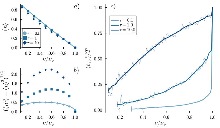
Figure E1: Comparing the effect of different correlation times on stationary statistics. Mean (a) and standard deviation (b) of stationary species abundances for different values of $\nu$. Markers are empirical values obtained from simulations, while solid line is the white noise limit analytic prediction. (c) Mean local time $\langle t_{<\varepsilon}\rangle$, i.e., mean length of time intervals spent by any species below a given threshold $\epsilon$ (in this case, $\epsilon=10^{-3}$), computed numerically; thick lines are smoothed (i.e. locally averaged) results, while thin dotted lines display typical fluctuations. As $\nu\to\nu_{c}$, mean local time saturates the observation time $T$, i.e., it diverges in the limit $T\to+\infty$, corresponding to the fact that all species become extinct at stationarity. Notice that different lines, representing mean local times for different values of $\tau$, begin at different values of $\nu/\nu_{c}$. This signals that, for $\nu\ll\nu_{c}$ and low $\tau$, no species will pass through the selected threshold. Correspondingly, we expect the peak of the SAD to move away from $n=0$.

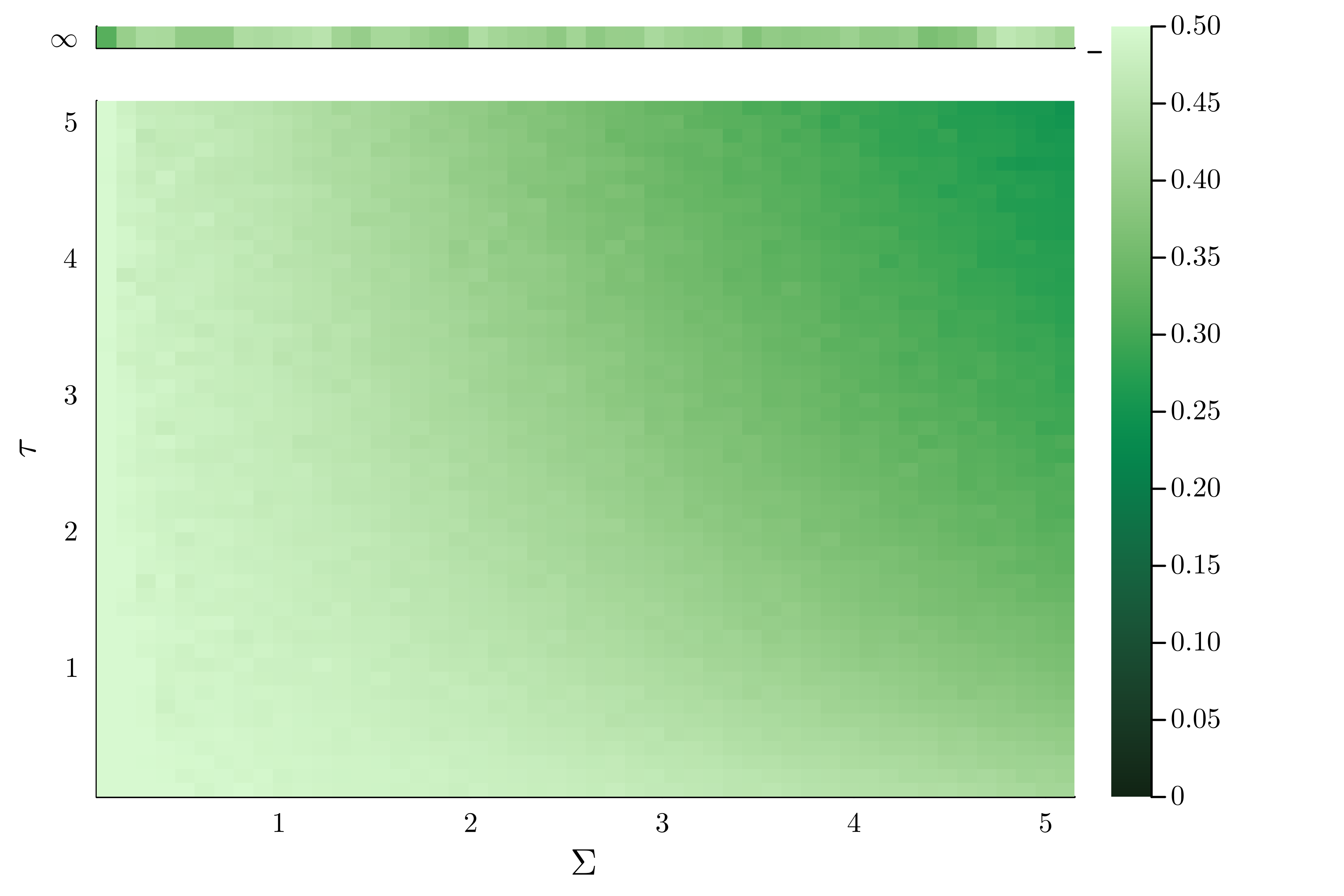
Figure E2: Evenness as function of $\Sigma$ and $\tau$, for $\Delta=0$; $\nu=1$. Each pixel is the result of a single realization of the system; the indicated value of evenness has been obtained by time average of the time dependent evenness, after discarding transients. The top line represents the corresponding values of evenness for the specified $\Sigma$ in the quenched limit, here realized with $\tau=10^{100}\approx\infty$. Notice that in the quenched limit evenness fluctuates widely, reflecting how the heterogeneity of steady state community structure depends on the realization of the system for relatively low $S$ and $R$. All parameters are reported in Appendix G.

Appendix F Stationary distributions for the case of abiotic resources

In general one might be interested in considering different types of dynamics for resources, in order to better represent different ecosystems. While stationary distribution of resources will change with its dynamics, the species abundance distribution will have the same form. As an important example, we consider abiotic dynamics for resources, namely the modification to Eqs. (1)

$$\dot{c}_{i}=\mu c_{i}(1-c_{i}/k)+\dots\rightarrow\dot{c}_{i}=\phi-\gamma c_{i}+\dots$$ (124)

The derivation of effective equations is identical to the case already considered, as is the study of stationary distributions for consumers and resources, which are identical in form to those in Eq. (7). However the coefficients of $p_{st}(c)$ are redefined to be $d_{c}=-2\frac{\gamma+\bar{\alpha}\langle n\rangle}{\Sigma^{2}\langle n^{2}\rangle}$, $b_{c}=\frac{\langle n^{2}\rangle}{\langle n\rangle}$ and $l_{c}=2\frac{\phi+\lambda_{c}}{\Sigma^{2}\langle n^{2}\rangle}$. Notice that $d_{c}<0$, while $l_{c}>0$ even in the case $\lambda_{c}=0$: this distribution is normalizable with $\mathcal{Z}_{c}^{-1}=2(b_{c}l_{c})^{d/2}K_{d}\Big{(}2\sqrt{l/b}\Big{)}$, where $K_{\cdot}(\cdot)$ is a modified Bessel function of the second kind. In fact the first two moments of the distributions can be written as $\langle c\rangle=\sqrt{b_{c}l_{c}}\frac{K_{1+d_{c}}\big{(}2\sqrt{l_{c}/b_{c}}\big{)}}{K_{d_{c}}\big{(}2\sqrt{l_{c}/b_{c}}\big{)}}$ and $\langle c^{2}\rangle=b_{c}l_{c}\frac{K_{2+d_{c}}\big{(}2\sqrt{l_{c}/b_{c}}\big{)}}{K_{d_{c}}\big{(}2\sqrt{l_{c}/b_{c}}\big{)}}$. In this case, self-consistent equations may only be solved numerically.

Appendix G Details on simulations and analysis

All code used to perform numerical analysis was written in Julia 1.9.3. All figures have been produced through the Plot.jl package, using the default GR backend. To fit curves to points, we used the function LsqFit.curve_fit, while to build hisogram from accumulated data we used Distributions.fit to populate an Histogram object. The random numbers used to build the trajectories of metabolic strategies have been generated through the function Base.randn(). Numerical integration of Eqs. 1 was performed through custom code, without using DifferentialEquations.jl or similar packages.

For $\tau>0$, we used the Euler-Maruyama scheme [68] to integrate the equations of motion, taking cautions that the integration step $dt$ is smaller than the correlation time $\tau$ by at least an order of magnitude, and in any case not larger than $10^{-2}$. While choosing smaller values of $\tau$ well approximates the white noise results, a rigorous analysis of the case $\tau=0$ requires that numerical integrations uses exactly white noise; in this limit, it is well known that one must use Stratonovich calculus [70], which is implemented numerically by Heun’s scheme [71]. In this case, choosing $dt=10^{-1}$ is often sufficient to obtain accurate results; however, as $\nu\to\nu_{c}$, smaller time steps are required to avoid abundances reaching 0 in finite times.

Initial conditions of both $n_{\sigma}$ and $c_{i}$ have been sampled by uniform distributions with support on positive real numbers, but stationary distributions has been found to be independent of initial conditions. Initial conditions of $Z_{\sigma,i}$ have been sampled from the stationary distribution of the corresponding Ornstein-Uhlenbeck process. Without this precaution, and especially in simulations for which $\tau\gtrapprox 10$ or $\nu\to\nu_{c}$, the time required for the system to reach the steady state may become exceedingly large.

To obtain numerically the stationary distributions to which compare those of the effective process, Eqs. (4), we simulated Eqs. (1) in a time interval $[0,T]$, and accumulated all values of $n_{\sigma}$ and $c_{i}$, after discarding all abundances in the transient time interval $[0,fT]$, with $0<f<1$. The choice of both $T$ and $f$ has been made on the empirical basis: as a thumb rule, larger values of $\tau$ lead to longer transients times to go from the initial distribution to the steady state distributions. Typically, for white noise simulations, we took $T=10^{3}$ and $f=0.5$, while for $\tau\gtrapprox 10$ we set $T=10^{4}$ and $f=0.7$. Furthermore, for large values of $\tau$, and due to long-lasting fluctuations, larger values of $S$ and $R$ need to be chosen, in order to adequately populate the empirical steady state distribution, so that comparisons with the analytical results are meaningful.

Figures: parameters used and additional notes

Fig. 1 Fixed parameters are $\bar{\alpha}=5$, $\Sigma=1$, $\Delta=0$, $\delta=1$, $\mu=10$, $\kappa=1$, $S=125$, $R=50$, $dt=10^{-2}$, $T=200$.

Fig. 2 (a) Fixed parameters are $\bar{\alpha}=10$, $\Sigma=1$, $\Delta=0$, $\delta=1$, $\mu=10$, $\kappa=1$, $R=50$, $dt=10^{-1}$, $T=5000$, $f=0.5$. Simulations have been carried out directly with white noise, i.e. not by choosing a value of $\tau$ close to 0. (b) Fixed parameters are $\bar{\alpha}=10$, $\Sigma=1$, $\Delta=0$, $\delta=1$, $\mu=10$, $\kappa=1$, $R=500$, $dt=10^{-1}$, $T=10^{4}$, $f\in[0.5,0.8]$ depending on $\tau$. Additionally, we report that, for large $\tau$, in order to successfully fit the theoretical distribution to empirical data, a suitable cut-off $\epsilon$ have to be applied to abundances, meaning that abundances lower than $\epsilon$ have not been accumulated to form empirical steady state distributions. For example, for $\tau=100$, we used $\epsilon=0.05$. The fit of the theoretical distribution has been performed using as free parameters both the constants $\chi_{x}$, $x=n,c$, as explained in the main text, and the normalization constants of the distributions.

Fig. 3 (a) Fixed parameters are $\bar{\alpha}=10$, $\Delta=0$, $\Sigma=\delta=\kappa=1$, $T=1000$, $dt=10^{-3}$, $f=0.7$ $R=100$.
(b) Fixed parameters are $\bar{\alpha}=10$, $\Delta=0$, $\Sigma=\delta=\kappa=1$, $\mu=100$, $T=1000$, $dt=\min\big{\{}10^{-2},\tau/10\big{\}}$, $f=0.7$ $R=500$.

Fig. 4 Fixed parameters are $\bar{\alpha}=10$, $\Sigma=\delta=\kappa=1$, $\tau=0.1$, $T=10^{3}$, $dt=10^{-2}$, $f=0.5$, $S=R=500$. (b) Fixed parameters are $\bar{\alpha}=50$, $\Delta=0.1$, $\delta=\kappa=1$, $T=5000$, $dt=10^{-2}$, $f=0.5$, $S=R=50$.

Fig. E1 Fixed parameters are $\bar{\alpha}=10$, $\delta=\kappa=1$, $\mu=10$. $T=1000$, $dt=10^{-2}$, $f=0.5$, $R=50$.

Fig. E2 Fixed parameters are $\bar{\alpha}=50$, $\Delta=0$, $\delta=\kappa=1$, $\mu=10$, $T=5000$, $dt=10^{-2}$, $f=0.5$, $S=R=50$.

References

- [1] Lawrence R Pomeroy and James J Alberts. Concepts of ecosystem ecology: a comparative view. Springer, 1988.
- [2] Edward O. Wilson. The diversity of life. Questions of science. Belknap Press of Harvard University Press Cambridge, Massachusetts, Cambridge, Massachusetts, 1992.
- [3] Robert M. May. How many species are there on earth? Science, 241(4872):1441–1449, 1988.
- [4] Paul L. Wennekes, James Rosindell, and Rampal S. Etienne. The neutral—niche debate: A philosophical perspective. Acta Biotheoretica, 60(3):257–271, Sep 2012.
- [5] Kevin S. McCann and Gabriel Gellner. Theoretical Ecology: concepts and applications. Oxford University Press, 05 2020.
- [6] Roger Arditi and Lev R Ginzburg. How species interact: altering the standard view on trophic ecology. Oxford University Press, 2012.
- [7] G. F. Gause. The Struggle for Existence. Williams & Wilkins, 1934.
- [8] G. Hardin. The competitive exclusion principle. Science, 131(3409):1292–1297, 1960.
- [9] Simon A. Levin. Community equilibria and stability, and an extension of the competitive exclusion principle. The American Naturalist, 104(939):413–423, 1970.
- [10] Robert H. MacArthur. Species packing and competitive equilibrium for many species. Theoretical Population Biology, 1(1):1–11, 1970.
- [11] Michael L. Rosenzweig and Robert H. MacArthur. Graphical representation and stability conditions of predator-prey interactions. The American Naturalist, 97(895):209–223, 1963.
- [12] David Tilman. Resource Competition and Community Structure. Princeton University Press, 1982.
- [13] Jonathan M. Chase and Mathew A. Leibold. Ecological Niches: Linking Classical and Contemporary Approaches. University of Chicago Press, 2003.
- [14] G. E. Hutchinson. The paradox of the plankton. The American Naturalist, 95(882):137–145, 1961.
- [15] Enrico Ser-Giacomi, Lucie Zinger, Shruti Malviya, Colomban De Vargas, Eric Karsenti, Chris Bowler, and Silvia De Monte. Ubiquitous abundance distribution of non-dominant plankton across the global ocean. Nature Ecology & Evolution, 2(8):1243–1249, Aug 2018.
- [16] Colomban de Vargas, Stéphane Audic, Nicolas Henry, Johan Decelle, Frédéric Mahé, Ramiro Logares, Enrique Lara, Cédric Berney, Noan Le Bescot, Ian Probert, Margaux Carmichael, Julie Poulain, Sarah Romac, Sébastien Colin, Jean-Marc Aury, Lucie Bittner, Samuel Chaffron, Micah Dunthorn, Stefan Engelen, Olga Flegontova, Lionel Guidi, Aleš Horák, Olivier Jaillon, Gipsi Lima-Mendez, Julius Lukeš, Shruti Malviya, Raphael Morard, Matthieu Mulot, Eleonora Scalco, Raffaele Siano, Flora Vincent, Adriana Zingone, Céline Dimier, Marc Picheral, Sarah Searson, Stefanie Kandels-Lewis, Tara Oceans Coordinators, Silvia G. Acinas, Peer Bork, Chris Bowler, Gabriel Gorsky, Nigel Grimsley, Pascal Hingamp, Daniele Iudicone, Fabrice Not, Hiroyuki Ogata, Stephane Pesant, Jeroen Raes, Michael E. Sieracki, Sabrina Speich, Lars Stemmann, Shinichi Sunagawa, Jean Weissenbach, Patrick Wincker, Eric Karsenti, Emmanuel Boss, Michael Follows, Lee Karp-Boss, Uros Krzic, Emmanuel G. Reynaud, Christian Sardet, Matthew B. Sullivan, and Didier Velayoudon. Eukaryotic plankton diversity in the sunlit ocean. Science, 348(6237):1261605, 2015.
- [17] Rolf Daniel. The metagenomics of soil. Nature Reviews Microbiology, 3(6):470–478, Jun 2005.
- [18] Alwyn H. Gentry. Tree species richness of upper amazonian forests. Proceedings of the National Academy of Sciences, 85(1):156–159, 1988.
- [19] Igor Volkov, Jayanth R. Banavar, Stephen P. Hubbell, and Amos Maritan. Patterns of relative species abundance in rainforests and coral reefs. Nature, 450(7166):45–49, Nov 2007.
- [20] Corey T. Callaghan, Luís Borda-de Água, Roel van Klink, Roberto Rozzi, and Henrique M. Pereira. Unveiling global species abundance distributions. Nature Ecology & Evolution, 7(10):1600–1609, Oct 2023.
- [21] Stephen P Hubbell. Tropical rain forest conservation and the twin challenges of diversity and rarity. Ecology and evolution, 3(10):3263–3274, 2013.
- [22] Egbert H van Nes, Diego GF Pujoni, Sudarshan A Shetty, Gerben Straatsma, Willem M de Vos, and Marten Scheffer. A tiny fraction of all species forms most of nature: Rarity as a sticky state. Proceedings of the National Academy of Sciences, 121(2):e2221791120, 2024.
- [23] Peter Chesson. Mechanisms of maintenance of species diversity. Annual Review of Ecology and Systematics, 31(1):343–366, 2000.
- [24] Jacopo Grilli. Macroecological laws describe variation and diversity in microbial communities. Nature Communications, 11(1):4743, Sep 2020.
- [25] Thomas W. Schoener. Resource partitioning in ecological communities. Science, 185(4145):27–39, 1974.
- [26] Yannis P. Papastamatiou, Bradley M. Wetherbee, Christopher G. Lowe, and Gerald L. Crow. Distribution and diet of four species of carcharhinid shark in the hawaiian islands: evidence for resource partitioning and competitive exclusion. Marine Ecology Progress Series, 320:239–251, 2006.
- [27] Thomas Pfeiffer and Sebastian Bonhoeffer. Evolution of cross-feeding in microbial populations. The American Naturalist, 163(6):E126–E135, 2004.
- [28] Joshua E. Goldford, Nanxi Lu, Djordje Bajić, Sylvie Estrela, Mikhail Tikhonov, Alicia Sanchez-Gorostiaga, Daniel Segrè, Pankaj Mehta, and Alvaro Sanchez. Emergent simplicity in microbial community assembly. Science, 361(6401):469–474, 2018.
- [29] Robert T. Paine. Food web complexity and species diversity. The American Naturalist, 100(910):65–75, 1966.
- [30] Jef Huisman and Franz J. Weissing. Biodiversity of plankton by species oscillations and chaos. Nature, 402(6760):407–410, Nov 1999.
- [31] Anna Posfai, Thibaud Taillefumier, and Ned S Wingreen. Metabolic trade-offs promote diversity in a model ecosystem. Physical review letters, 118(2):028103, 2017.
- [32] Deepak Gupta, Stefano Garlaschi, Samir Suweis, Sandro Azaele, and Amos Maritan. Effective resource competition model for species coexistence. Phys. Rev. Lett., 127:208101, Nov 2021.
- [33] Yizhou Liu, Jiliang Hu, and Jeff Gore. Ecosystem stability relies on diversity difference between trophic levels. Proceedings of the National Academy of Sciences, 121(50):e2416740121, 2024.
- [34] Leonardo Pacciani-Mori, Andrea Giometto, Samir Suweis, and Amos Maritan. Dynamic metabolic adaptation can promote species coexistence in competitive microbial communities. PLOS Computational Biology, 16(5):1–18, 05 2020.
- [35] Russell Lande, Steinar Engen, and Bernt-Erik SÆther. 1demographic and environmental stochasticity. In Stochastic Population Dynamics in Ecology and Conservation. Oxford University Press, 04 2003.
- [36] Masakazu Shimada, Yumiko Ishii, and Harunobu Shibao. Rapid adaptation: a new dimension for evolutionary perspectives in ecology. Population ecology, 52:5–14, 2010.
- [37] David Raubenheimer, Stephen J Simpson, and Alice H Tait. Match and mismatch: conservation physiology, nutritional ecology and the timescales of biological adaptation. Philosophical Transactions of the Royal Society B: Biological Sciences, 367(1596):1628–1646, 2012.
- [38] Sylvain Giroud, Andreas Nord, Kenneth B. Storey, and Julia Nowack. Editorial: Coping with environmental fluctuations: Ecological and evolutionary perspectives. Frontiers in Physiology, 11, October 2020.
- [39] Liliana Pinek, India Mansour, Milica Lakovic, Masahiro Ryo, and Matthias C Rillig. Rate of environmental change across scales in ecology. Biological Reviews, 95(6):1798–1811, 2020.
- [40] Joey R. Bernhardt, Mary I. O’Connor, Jennifer M. Sunday, and Andrew Gonzalez. Life in fluctuating environments. Philosophical Transactions of the Royal Society B: Biological Sciences, 375(1814):20190454, November 2020.
- [41] Nelson G Hairston Jr, Stephen P Ellner, Monica A Geber, Takehito Yoshida, and Jennifer A Fox. Rapid evolution and the convergence of ecological and evolutionary time. Ecology letters, 8(10):1114–1127, 2005.
- [42] Scott P Carroll, Andrew P Hendry, David N Reznick, and Charles W Fox. Evolution on ecological time-scales, 2007.
- [43] Emanuel A Fronhofer, Dov Corenblit, Jhelam N Deshpande, Lynn Govaert, Philippe Huneman, Frédérique Viard, Philippe Jarne, and Sara Puijalon. Eco-evolution from deep time to contemporary dynamics: The role of timescales and rate modulators. Ecology Letters, 26:S91–S108, 2023.
- [44] Andrew Morozov, Karen Abbott, Kim Cuddington, Tessa Francis, Gabriel Gellner, Alan Hastings, Ying-Cheng Lai, Sergei Petrovskii, Katherine Scranton, and Mary Lou Zeeman. Long transients in ecology: Theory and applications. Physics of life reviews, 32:1–40, 2020.
- [45] R. H. MacArthur. Population ecology of some warblers of northeastern coniferous forests. Ecology, 39(4):599–619.
- [46] J. H. Connell. Diversity in tropical rain forests and coral reefs. Science, 199(4335):1302–1310, 1978.
- [47] Christopher A Klausmeier. Successional state dynamics: a novel approach to modeling nonequilibrium foodweb dynamics. Journal of Theoretical Biology, 262(4):584–595, 2010.
- [48] Jeremy W Fox. The intermediate disturbance hypothesis should be abandoned. Trends in ecology & evolution, 28(2):86–92, 2013.
- [49] Douglas Sheil and David FRP Burslem. Defining and defending connell’s intermediate disturbance hypothesis: a response to fox. Trends in ecology & evolution, 28(10):571–572, 2013.
- [50] Jeremy W Fox. The intermediate disturbance hypothesis is broadly defined, substantive issues are key: a reply to sheil and burslem. Trends in Ecology & Evolution, 28(10):572–573, 2013.
- [51] Sandro Azaele and Amos Maritan. Generalized dynamical mean field theory for non-gaussian interactions. Phys. Rev. Lett., 133:127401, Sep 2024.
- [52] Samir Suweis, Francesco Ferraro, Christian Grilletta, Sandro Azaele, and Amos Maritan. Generalized lotka-volterra systems with time correlated stochastic interactions. Phys. Rev. Lett., 133:167101, Oct 2024.
- [53] F Roy, G Biroli, G Bunin, and C Cammarota. Numerical implementation of dynamical mean field theory for disordered systems: application to the lotka–volterra model of ecosystems. Journal of Physics A: Mathematical and Theoretical, 52(48):484001, nov 2019.
- [54] Tobias Galla. Dynamically evolved community size and stability of random lotka-volterra ecosystems(a). EPL (Europhysics Letters), 123(4):48004, September 2018.
- [55] Madhu Advani, Guy Bunin, and Pankaj Mehta. Statistical physics of community ecology: a cavity solution to macarthur’s consumer resource model. Journal of Statistical Mechanics: Theory and Experiment, 2018(3):033406, mar 2018.
- [56] A. R. Batista-Tomás, Andrea De Martino, and Roberto Mulet. Path-integral solution of macarthur’s resource-competition model for large ecosystems with random species-resources couplings. Chaos: An Interdisciplinary Journal of Nonlinear Science, 31(10), October 2021.
- [57] Peter Jung and Peter Hänggi. Dynamical systems: A unified colored-noise approximation. Physical Review A, 35(10):4464–4466, May 1987.
- [58] Frank W Preston. The commonness, and rarity, of species. Ecology, 29(3):254–283, 1948.
- [59] Anna Tovo, Samir Suweis, Marco Formentin, Marco Favretti, Igor Volkov, Jayanth R Banavar, Sandro Azaele, and Amos Maritan. Upscaling species richness and abundances in tropical forests. Science advances, 3(10):e1701438, 2017.
- [60] Thierry Mora and Aleksandra M Walczak. Rényi entropy, abundance distribution, and the equivalence of ensembles. Physical Review E, 93(5):052418, 2016.
- [61] Davide Zanchetta, Amos Maritan, and Sandro Azaele. Modelling post-disturbance empirical patterns in a forest ecosystem. bioRxiv, 2024.
- [62] Iris … Hordijk. Evenness mediates the global relationship between forest productivity and richness. Journal of Ecology, 111(6):1308–1326, May 2023.
- [63] Emanuele Pigani, Bruno Hay Mele, Lucia Campese, Enrico Ser-Giacomi, Maurizio Ribera, Daniele Iudicone, and Samir Suweis. Deviation from neutral species abundance distributions unveils geographical differences in the structure of diatom communities. Science Advances, 10(10), March 2024.
- [64] Benjamin Smith and J. Bastow Wilson. A consumer’s guide to evenness indices. Oikos, 76(1):70, May 1996.
- [65] Brian J. Wilsey and Catherine Potvin. Biodiversity and ecosystem functioning: Importance of species evenness in an old field. Ecology, 81(4):887–892, April 2000.
- [66] Sandro Azaele, Samir Suweis, Jacopo Grilli, Igor Volkov, Jayanth R Banavar, and Amos Maritan. Statistical mechanics of ecological systems: Neutral theory and beyond. Reviews of Modern Physics, 88(3):035003, 2016.
- [67] Samir Suweis, Francesco Ferraro, Christian Grilletta, Sandro Azaele, and Amos Maritan. Generalized lotka-volterra systems with time correlated stochastic interactions. Physical Review Letters, 133(16):167101, 2024.
- [68] C. W. Gardiner. Handbook of stochastic methods for physics, chemistry and the natural sciences. Berlin, 2004.
- [69] Ian F. Spellerberg and Peter J. Fedor. A tribute to claude shannon (1916–2001) and a plea for more rigorous use of species richness, species diversity and the ‘shannon–wiener’ index. Global Ecology and Biogeography, 12(3):177–179, April 2003.
- [70] NG Van Kampen. Stochastic Processes in Physics and Chemistry. North-Holland Publishing Co, 1992.
- [71] W Rüemelin. Numerical treatment of stochastic differential equations. SIAM Journal on Numerical Analysis, 19(3):604–613, 1982.