Hierarchical RL-MPC for Demand Response Scheduling
Abstract
This paper presents a hierarchical framework for demand response optimization in air separation units (ASUs) that combines reinforcement learning (RL) with linear model predictive control (LMPC). We investigate two control architectures: a direct RL approach and a control-informed methodology where an RL agent provides setpoints to a lower-level LMPC. The proposed RL-LMPC framework demonstrates improved sample efficiency during training and better constraint satisfaction compared to direct RL control. Using an industrial ASU case study, we show that our approach successfully manages operational constraints while optimizing electricity costs under time-varying pricing. Results indicate that the RL-LMPC architecture achieves comparable economic performance to direct RL while providing better robustness and requiring fewer training samples to converge. The framework offers a practical solution for implementing flexible operation strategies in process industries, bridging the gap between data-driven methods and traditional control approaches.
keywords:
Reinforcement learning, Chemical process control, Production scheduling1 Introduction
The growing proportion of renewable energy sources in power grids has led to greater volatility in electricity prices and supply. This creates both challenges and opportunities for energy-intensive industries. Demand response (DR) programs, which incentivize consumers to adjust their electricity usage in response to grid conditions, have emerged as a crucial tool for maintaining grid stability and efficiency. In this context, developing and operating flexible processes that can modulate their power consumption without compromising product quality or operational safety has become a key focus. Air separation units (ASUs), which produce high-purity oxygen, nitrogen, and argon from atmospheric air, are prime candidates for implementing DR strategies. These facilities consume significant amounts of electricity, amounting to 2.55% of U.S. manufacturing sector electricity (Pattison et al., 2016), and their products can be stored cryogenically, allowing for temporal decoupling of production and demand. However, the complex dynamics and strict operational constraints of ASUs pose challenges for DR implementation.
Optimization-based methods have been widely studied for ASU scheduling and control in DR contexts. Recent work has explored top-down approaches, e.g., using scale-bridging models with linear MPC (LMPC) and bottom-up strategies, e.g., employing economic nonlinear MPC (eNMPC). While these methods have shown promise, they face limitations in practical implementation. They rely on accurate process models, which can be challenging to develop and maintain for ASUs (Tsay et al., 2019). Additionally, computational solution of large-scale optimization problems in real time can be prohibitive (Caspari et al., 2020). Reinforcement learning (RL) offers an alternative, data-driven approach that can potentially overcome some of these limitations. RL agents can learn to approximate optimal control policies directly from process data and interactions. Once trained, RL policies generally enable quick real-time inference, avoiding the computational burden of online optimization. However, the direct application of RL to complex chemical processes such as ASUs faces challenges in terms of sample efficiency, stability, and constraint satisfaction. In this work, we propose a practical method that combines the strengths of RL and MPC for ASU control in DR scenarios. Specifically, we investigate a hierarchical framework that integrates the scheduling decisions of an RL agent with a lower-level LMPC system. We opt for linear MPC over nonlinear MPC due to its faster inference time, ensuring it doesn’t detract from RL’s computational efficiency, though this comes at the cost of some control performance. This approach aims to leverage RL’s learning capabilities and forward-inference efficiency while benefiting from MPC’s stabilizing effect on the learning process.
1.1 Related Works
The DR problem for industrial processes falls within the broader class of enterprise-wide optimization (EWO) problems described by Flores-Tlacuahuac and Grossmann (2006). In the context of DR, this often involves solving complex mixed-integer dynamic optimization (MIDO) problems, which combine discrete decisions (e.g., product scheduling) with continuous dynamic process models. These problems are typically transformed into mixed-integer nonlinear programming (MINLP) formulations for solution. While MIDO and MINLP approaches offer a rigorous framework for integrating scheduling and control decisions (Zhang et al., 2015), they often face computational challenges due to problem size and complexity.
Pattison et al. (2016) introduced scale-bridging models (SBMs) for DR applications, using data-driven low-order dynamic models to ensure feasible schedules with reduced computational burden. The approach demonstrated significant cost savings when applied to an air separation unit under time-varying electricity prices. Building on this work, Dias et al. (2018), Caspari et al. (2020), and Schulze et al. (2023) compared different paradigms for integrating scheduling and control in DR problems. Dias et al. developed a simulation-based optimization framework that combines SBMs with model predictive control (MPC), while Caspari et al. contrasted this “top-down” approach with a “bottom-up” economic MPC formulation. Schulze et al. developed a Koopman-based approach achieving real-time NMPC with 98% reduced computational cost. Applied to an air separation unit, this method demonstrated 8% cost savings over steady-state operation, though highlighting tradeoffs between computational efficiency and economic optimality.
Reinforcement learning (RL) presents a compelling approach to demand response in industrial processes, offering advantages over traditional optimization methods. RL learns optimal control policies through environment interaction without requiring explicit mathematical models of system dynamics or constraints. Its effectiveness has been demonstrated in industrial applications, particularly in fed-batch bioreactors (Kaisare et al., 2003; Peroni et al., 2005), which present significant run-to-run variabilities (Yoo et al., 2021; Petsagkourakis et al., 2022). Recent advances include integrating RL with PID controllers for improved interpretability and sample efficiency (Lawrence et al., 2022), with Bloor et al. (2024) showing enhanced performance through combined neural network-PID architectures. The data-driven nature of RL complements scheduling-based modeling approaches by leveraging historical data to improve decision-making. While challenges such as sample efficiency and stability remain, modern approaches such as scalable algorithms through action-space dimensionality reduction (Zhu et al., 2020) and hierarchical RL frameworks have shown promise in industrial control applications, as demonstrated by Kim et al. (2023) in optimal continuous control of refrigeration systems under Time-of-Use pricing. While these previous works have demonstrated the potential of both traditional optimization and reinforcement learning approaches, the integration of RL with MPC for demand response optimization remains largely unexplored. Our work addresses this gap by presenting a hierarchical framework that combines reinforcement learning with LMPC, demonstrating enhanced sample efficiency and constraint satisfaction while maintaining economic performance in industrial demand response applications.
2 Methodology
2.1 Reinforcement Learning for Control
In the RL framework, an agent learns to make decisions by interacting with an environment, aiming to maximize a cumulative reward signal. Formally, RL problems are often modeled as Markov Decision Processes (MDPs), defined by the tuple . Here, represents the state space, and is the control input space. The transition function describes the (stochastic) dynamics of the environment, while the reward function quantifies the desirability of transitions. The discount factor balances immediate and future rewards.
The goal in RL is to find the policy that maximizes the expected cumulative discounted reward:
| (1) |
where , , and the expectation is taken over the trajectories induced by the policy and the environment dynamics .
2.2 RL Control Structure
In this work, we explore two methodologies for applying RL to process control: a direct formulation and a control-informed approach. The following are formulated in a deterministic setting, in terms of both the dynamics, , and the control policy, .
In the direct, control-agnostic formulation, we train an RL agent to directly output control actions. The optimization problem can be formulated as:
| s.t. | |||
where are the differential states, and the deterministic system dynamics correspond to the process model, which is represented as a semi-explicit differential algebraic equation (DAE) system.
The hierarchical, control-informed approach combines the strengths of RL and LMPC. This formulation assumes the availability of a linear model of the plant, typically obtained from previous control experiments or system identification. In this framework, the RL agent learns to provide setpoints to a lower-level LMPC system. The optimization problem becomes:
| s.t. | |||
In this case, represents the RL policy that provides setpoints to the control law (written explicitly for simplicity), which then in turn determines the control actions . In this work, the control law is represented by a lower-level LMPC optimization that solves a quadratic program at each timestep to track the RL-provided setpoints. We employ the process model, linear dynamics, and cost matrices provided by Dias et al. (2018). While LMPC is chosen for its computational efficiency, its linear approximation of the nonlinear ASU dynamics can limit control performance, particularly during large transitions.
2.3 Constraint Handling
While recent works investigate directly embedding constraints in RL (Burtea and Tsay, 2024), here we simply formulate operational constraints of the problem as penalties to the reward function. For a path constraint of the form , the penalty at time is defined as:
| (2) |
where represents the nonlinear constraint function and represents a scaling factor to weight the constraints. For a terminal constraint of the form , we can densify the reward signal by relaxing it to a path constraint that activates when :
| (3) |
where represents the terminal constraint function evaluated at time , and represents the activation time, selected to balance effective load shifting influence and a sufficient response time for the agent. This modification provides continuous feedback throughout the latter portion of the episode instead of only at the terminal time . Equality constraints can be treated by duplicating (2)–(3).
2.4 Policy Optimization
Policy optimization is a fundamental approach in RL for finding an optimal policy. In continuous action spaces, policy gradient methods have shown significant promise. Among these, the Deep Deterministic Policy Gradient (DDPG) algorithm has emerged as particularly effective for continuous control tasks (Lillicrap et al., 2019), and we employ this algorithm for policy optimization throughout this work, although the proposed method is agnostic to the choice of RL algorithm. DDPG combines elements of both policy-based and value-based methods, utilizing an actor-critic architecture. Central to this approach is the concept of the Q-function, also known as the action-value function. The Q-function is defined as the expected cumulative discounted reward when taking action in state and following policy thereafter:
| (4) |
where is the reward at time step . In complex environments with continuous or high-dimensional state and action spaces, the Q-function can be approximated using a neural network:
| (5) |
where represents the parameters of the neural network. Building on these concepts, DDPG learns a deterministic policy and an action-value function simultaneously. The objective is to maximize the expected return defined as:
| (6) |
where is the deterministic policy. The policy is updated using the deterministic policy gradient theorem:
| (7) |
where are the parameters of the policy network, are the parameters of the Q-function network, and is the state distribution under the behavior policy .
3 Computational Case Study
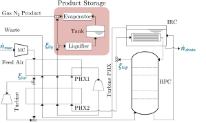
The ASU used as the case study within this work is an openly available benchmark process for flexible operation problems (Tsay et al., 2020) and is depicted in Figure 2. This benchmark process represents the environment that both agents can interact with. The ASU’s main process unit is the single cryogenic distillation column which produces high-purity Nitrogen product. The feed air () is passed through an electric compressor (MC in Figure 2) and is cooled in the first Primary Heat Exchanger (PHX1) after which a fraction is sent to the turbine to generate electricity. The rest of the feed is sent to the second Primary Heat Exchanger 2 (PHX2). This liquified stream is combined with the turbine outlet to feed the High Pressure Column (HPC). The bottoms stream is then sent to the reboiler side of the Integrated Reboiler/Condenser (IRC) Unit. The high-purity nitrogen from the distillate is split by fraction and sent to the primary heat exchanger. To enable the flexible operation of the ASU, nitrogen product can be liquified and sent to the storage tank. This stored product can be evaporated to meet the instantaneous demand when the production rate is decreased allowing the shifting of load. The fraction sent to the liquified is set with the following control logic so that the product demand is met at all times:
| (8) |
For a detailed explanation of the modeling of the ASU, we direct the reader to the work by Caspari et al. (2020).
3.1 Operational Constraints
The ASU system must be controlled to satisfy certain operational constraints regarding product purity, heat exchanger minimum temperature difference, and vessel holdup. Along with these constraints is a terminal constraints on the storage tank holdup. The storage constraint in particular is enforced to ensure enough storage for the following days. We note that this constraint is artificial since, over a long time horizon, it may be optimal to finish the horizon at lower or higher storage holdups dependent on the following day’s electricity profile and demand. The specific enforced path and terminal constraints are shown in Table 1 and the manipulated variable bounds are shown in Table 2.
| Variable | Constraint | Type |
|---|---|---|
| [ppm] | Path | |
| [K] | Path | |
| [mol] | Path | |
| [mol/s] | Path | |
| [mol | Terminal |
| MV | Bounds |
|---|---|
| [mol/s] | |
| [-] | |
| [-] | |
| [-] | |
| [mol/s] |
3.2 Reward Function
The objective of the case study is to minimize operational costs while also satisfying operational constraints. To translate this to the RL framework, we must construct a reward function that describes this goal. The economic half of the objective can be described as the maximization of the negative electricity costs as follows:
| (9) |
where [$/MWh] the electricity price at time , and [MW] is the power consumed/generated by unit at time step . The total reward at each timestep can then be written as:
| (10) |
3.3 State and Action Spaces
The RL agent’s state space is designed to contain the relevant information to make decisions. For both RL agents described in Section 2.2 the state is defined as:
| (11) |
where [ppm] is the product impurity, [K] is the temperature difference in the internal rectification column, [mol] is the amount of product in the storage tank, [mol/s] is the flow rate to the storage tank, [$/MWh] represents the electricity prices for the next 12 hours (perfect forecast is assumed), and represents the time within the day.
For the direct RL agent, the action space consists of all manipulated variables:
| (12) |
where [mol/s] is the main air compressor flow rate, [-] is the turbine split fraction, [-] is the top column split fraction, and [mol/s] is the reboiler drain flow rate. For the RL-LMPC agent, the action space is reduced to a single setpoint:
| (13) |
where [mol/s] is the setpoint for the product flow rate. Since the LMPC can effectively maintain the other three controlled variables around their steady-state values through coordinated manipulation of the lower-level inputs, we can reduce the action space from to . This simplification of the action space dimensionality allows the RL agent to focus solely on the critical production rate decisions while relying on the LMPC for stable operation of the remaining process variables.
4 Results and Discussion
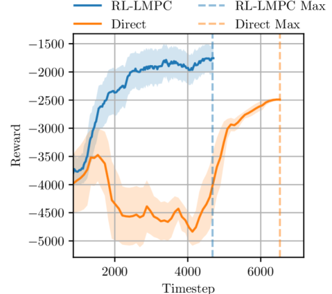
Figure 3 presents the learning curves for both RL-control approaches. Both algorithms were implemented using the Stable-Baselines3 library by Raffin et al. (2021), with default hyperparameters and trained with a budget of 10,000 timesteps and episodes of 96 timesteps, corresponding to a single day. The RL-LMPC framework demonstrates more efficient learning by converging to a high-quality policy after approximately 4000 timesteps, while the direct RL method required nearly 7000 timesteps to improve its final performance. This faster learning rate of the RL-LMPC can be attributed to the embedded LMPC reducing the exploration space by handling constraints explicitly, thereby allowing the RL agent to focus on optimizing the control policy within a feasible operating region. Moreover, the dimensionality of the explored action space is reduced considerably. After training, the best policy achieved within the 10,000 timestep budget was fixed and used to generate the subsequent operational trajectories shown in Figures 4 and 5.

Figure 4 first shows the power demand of the ASU unit overlayed over the electricity price profile and the product flow rates for both direct and RL-LMPC agents. Both control policies exhibit load-shifting behavior, strategically reducing power consumption during periods of peak electricity prices and increasing production during lower-price periods. The direct RL policy adopts a more conservative approach during the first 10 hours of operation, maintaining power consumption between 0.300-0.330 MW, despite relatively favorable electricity prices. In contrast, within the same period, the RL-LMPC increases production in preparation for the high energy prices. During the latter half of the operating period (hours 10-20), the direct policy becomes more aggressive, showing significant variations in power consumption in response to price fluctuations and the terminal storage constraint. While the RL-LMPC demonstrates effective load-shifting, some of its responses appear more aggressive than necessary, which may be attributed to the current LMPC tuning parameters rather than fundamental limitations of the approach. This follows the observations of Caspari et al. (2020) that allowing a scheduling layer to control the setpoints directly can give the flexibility to enable more aggressive behavior.
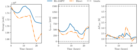
Figure 5 presents the trajectories of three constrained variables: storage levels, product impurity, and IRC temperature differences, comparing the performance of RL-LMPC and direct RL control approaches. The storage trajectory is subject to a terminal constraint requiring a return to the mid-level by the end of the 24-hour period. Both control approaches fail to satisfy this terminal condition, though with markedly different magnitudes. The direct RL agent exhibits substantially larger deviations, primarily due to its conservative operating strategy during initial hours, which fails to build a sufficient storage buffer for subsequent operations. The RL-LMPC agent, while still violating the terminal constraint, maintains closer proximity to the desired final state.
In terms of path constraints, both agents successfully maintain product impurity within the specified bounds throughout the operational period. However, a significant performance divergence occurs in the IRC temperature difference at hour 20, where the direct RL agent notably violates the lower bound. The RL-LMPC agent, benefiting from its embedded linear constraint model in the lower-level LMPC, successfully avoids such violations. This superior performance stems from the LMPC’s explicit constraint handling mechanism, which reduces constraint-violating actions from the RL agent’s exploration space, demonstrating a key advantage of the hybrid approach in managing operational constraints.
5 Conclusions and Future Works
This work investigates integrating reinforcement learning with model predictive control for demand response scheduling in air separation units. The proposed RL-LMPC framework showed certain advantages over a direct RL implementation in terms of sample efficiency and constraint satisfaction. By incorporating the LMPC’s knowledge of system dynamics and constraints, the hybrid approach reduces the solution space for the RL agent, helping avoid some infeasible operating conditions. This reduction in searchable space contributed to more efficient learning and we found the hybrid approach to exhibit more stable control behavior. Both approaches implemented load-shifting strategies in response to electricity price variations, with the RL-LMPC framework showing better capability at maintaining feasible operation.
Future work may investigate fully RL-based hierarchical control structures, e.g., where both high-level and low-level controllers are RL agents. The framework can be extended to incorporate stochastic electricity price distributions and varying initial storage levels. These developments may help advance the practical implementation of RL-based strategies in industrial process scheduling.
References
- Bloor et al. (2024) Bloor, M., Ahmed, A., Kotecha, N., Mercangöz, M., Tsay, C., and Chanona, E.A.D.R. (2024). Control-informed reinforcement learning for chemical processes. arXiv:2408.13566.
- Burtea and Tsay (2024) Burtea, R. and Tsay, C. (2024). Constrained continuous-action reinforcement learning for supply chain inventory management. Comput. Chem. Eng., 181, 108518.
- Caspari et al. (2020) Caspari, A., Tsay, C., Mhamdi, A., Baldea, M., and Mitsos, A. (2020). The integration of scheduling and control: Top-down vs. bottom-up. J. Process Control, 91, 50–62.
- Dias et al. (2018) Dias, L.S., Pattison, R.C., Tsay, C., Baldea, M., and Ierapetritou, M.G. (2018). A simulation-based optimization framework for integrating scheduling and model predictive control, and its application to air separation units. Comput. Chem. Eng., 113, 139–151.
- Flores-Tlacuahuac and Grossmann (2006) Flores-Tlacuahuac, A. and Grossmann, I.E. (2006). Simultaneous Cyclic Scheduling and Control of a Multiproduct CSTR. Ind. Eng. Chem. Res., 45(20), 6698–6712.
- Kaisare et al. (2003) Kaisare, N.S., Lee, J.M., and Lee, J.H. (2003). Simulation based strategy for nonlinear optimal control: Application to a microbial cell reactor. Int. J. Robust and Nonlinear Control, 13(3-4), 347–363.
- Kim et al. (2023) Kim, B., An, J., and Sim, M.K. (2023). Optimal continuous control of refrigerator for electricity cost minimization—Hierarchical reinforcement learning approach. Sustain. Energy Grids Netw., 36, 101177.
- Lawrence et al. (2022) Lawrence, N.P., Forbes, M.G., Loewen, P.D., McClement, D.G., Backström, J.U., and Gopaluni, R.B. (2022). Deep reinforcement learning with shallow controllers: An experimental application to PID tuning. Control Eng. Pract., 121, 105046.
- Lillicrap et al. (2019) Lillicrap, T.P., Hunt, J.J., Pritzel, A., Heess, N., Erez, T., Tassa, Y., Silver, D., and Wierstra, D. (2019). Continuous control with deep reinforcement learning. arXiv:1509.02971.
- Pattison et al. (2016) Pattison, R.C., Touretzky, C.R., Johansson, T., Harjunkoski, I., and Baldea, M. (2016). Optimal process operations in fast-changing electricity markets: Framework for scheduling with low-order dynamic models and an air separation application. Ind. Eng. Chem. Res., 55(16), 4562–4584.
- Peroni et al. (2005) Peroni, C.V., Kaisare, N.S., and Lee, J.H. (2005). Optimal control of a fed-batch bioreactor using simulation-based approximate dynamic programming. IEEE Trans. Control Syst. Technol., 13(5), 786–790.
- Petsagkourakis et al. (2022) Petsagkourakis, P., Sandoval, I.O., Bradford, E., Galvanin, F., Zhang, D., and del Rio-Chanona, E.A. (2022). Chance constrained policy optimization for process control and optimization. Journal of Process Control, 111, 35–45.
- Raffin et al. (2021) Raffin, A., Hill, A., Gleave, A., Kanervisto, A., Ernestus, M., and Dormann, N. (2021). Stable-baselines3: Reliable reinforcement learning implementations. Journal of Machine Learning Research, 22(268), 1–8. URL http://jmlr.org/papers/v22/20-1364.html.
- Schulze et al. (2023) Schulze, J.C., Doncevic, D.T., Erwes, N., and Mitsos, A. (2023). Data-driven model reduction and nonlinear model predictive control of an air separation unit by applied Koopman theory. arXiv:2309.05386.
- Tsay et al. (2020) Tsay, C., Caspari, A., Pattison, R., Johansson, T., Mitsos, A., and Baldea, M. (2020). A benchmark air separation unit for process control and flexible operation. Mendeley Data v1, 2. Doi:10.17632/pfcc5gvzty.1.
- Tsay et al. (2019) Tsay, C., Kumar, A., Flores-Cerrillo, J., and Baldea, M. (2019). Optimal demand response scheduling of an industrial air separation unit using data-driven dynamic models. Comput. Chem. Eng., 126, 22–34.
- Yoo et al. (2021) Yoo, H., Byun, H.E., Han, D., and Lee, J.H. (2021). Reinforcement learning for batch process control: Review and perspectives. Annu. Rev. Control, 52, 108–119.
- Zhang et al. (2015) Zhang, Q., Grossmann, I.E., Heuberger, C.F., Sundaramoorthy, A., and Pinto, J.M. (2015). Air separation with cryogenic energy storage: optimal scheduling considering electric energy and reserve markets. AIChE J., 61(5), 1547–1558.
- Zhu et al. (2020) Zhu, L., Cui, Y., Takami, G., Kanokogi, H., and Matsubara, T. (2020). Scalable reinforcement learning for plant-wide control of vinyl acetate monomer process. Control Eng. Pract., 97, 104331.