Natural damping of time-harmonic waves and its influence on Schwarz methods
1 Introduction
The Helmholtz equation is often used as the prototype time harmonic problem which is difficult to solve by numerical methods, both because high mesh resolutions are required when the wave number becomes large and iterative solvers struggle to solve such discretized problems ernst2011difficult . An idea is to use the shifted Helmholtz equation van2007spectral , , also called the Helmholtz equation with damping, and the parameter can be chosen to make iterative methods succeed, even though a difficult compromise must be chosen between approximation of the Helmholtz equation solution ( gander2015applying ) and easy solvability by iterative methods ( cocquet2017large ) when using the shifted problem as a preconditioner.
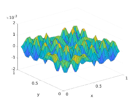
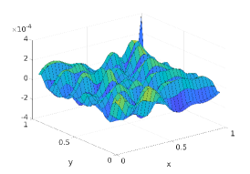
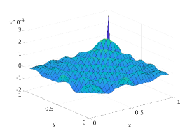
It was shown in Gander_Zhang_2022 that important damping is also coming from the outer boundary conditions applied to the Helmholtz equation, and while it is the closed cavity (all Dirichlet) and the waveguide (Dirichlet along the guide and impedance at the ends) are the really hard to solve by iterative methods, the free space problem (e.g. impedance all around) becomes as easy to solve as the Laplace problem in the constant coefficient case for Schwarz methods of sweeping type gander2019class based on optimized Schwarz technology. We show in Fig. 1 a Greens function corresponding to these three cases to illustrate how different the solution looks like.
We are interested here in studying if natural damping mechanisms coming from the physical properties of the wave phenomenon one wants to study can make the damped Helmholtz problem easy to solve by such Schwarz methods. To do so, we go back to the underlying phyiscal wave equation from which the Helmholtz equation arises, namely the second order wave equation, . There are two main damping mechanisms that arise in nature for damping solutions of the second order wave equation, first order and viscoelastic damping,
| (1) |
where is the first order damping strength, and is the viscoelastic damping strength. These terms are present in all physical phenomena in nature, the second order wave equation is a simplifying model, and waves never remain forever, there is always damping. If the source and the solution have the time-harmonic form and , then we find , which we write it in the normalized form (omitting the hats) to obtain the new Helmholtz equation that includes natural damping,
| (2) |
We show in Figure 2 the influence of first order and viscoelastic damping on the Greens functions from Figure 1.
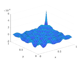
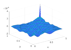

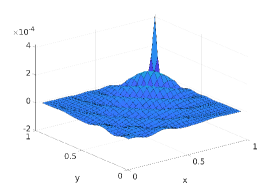
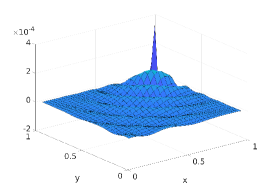
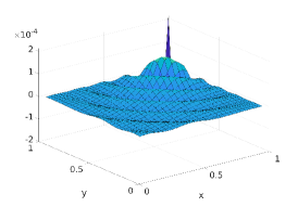
We see that both types of damping make the Greens function look like the easy to solve case in Figure 1 on the right, all difficulties from the closed cavity and wave guide configurations seem to have disappeared. It is therefore of interest to investigate the performance of Schwarz methods in these naturally damped configurations.
We analyze here the parallel Schwarz method applied to (2) on the domain with impedance transmission conditions at subdomain interfaces of the form , where is the unit normal. We decompose the domain along the direction into overlapping subdomains of the same width with the overlap width shared by two neighbors. We apply Fourier series in , then calculate the spectral radius of the iteration matrix of the interface values , which we call convergence factor , and present results both for the waveguide and the closed cavity problems.
2 Waveguide problem
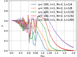
In the waveguide problem, at , and on the other sides, and we consider first order damping (, ) and viscoelastic damping (, ) separately. We visualize the convergence factor in the Fourier domain with the Fourier frequency for .
2.1 Helmholtz operator in the waveguide
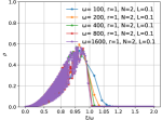
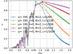
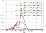
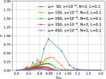
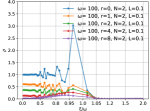
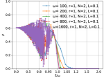
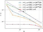
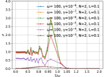
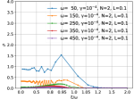
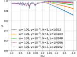
We first measure how the convergence factor scales with the damping coefficient ; see Fig. 3.
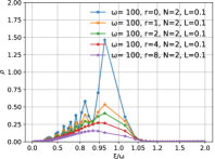
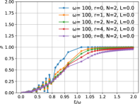
We see that the damping helps not only convergence of the propagating modes () but also the evanescent modes (), and that the benefit is more notable for the nonoverlapping method () and its evanescent modes. On the right, we see that the convergence factor goes to zero exponentially when , indicating very fast convergence.
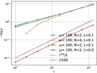
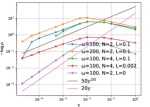
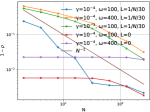
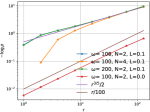
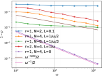
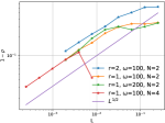
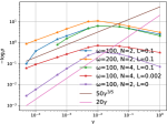
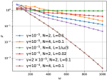
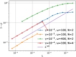
Next, we study the scalings with respect to the wavenumber , number of subdomains and the overlap width . On many subdomains, the overlap width has to be sufficiently small with respect to the wavenumber and the number of subdomains to ensure convergence without physical damping Gander_Zhang_2022 . Actually, for each given and , there would be an optimal overlap width, but we will not seek the optimal in this note and just use an ad hoc choice. Fig. 4
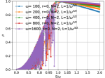
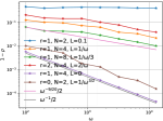
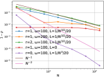
show that the waveguide problem with first order damping has similar scalings to the free space problem without damping in Gander_Zhang_2022 , while the waveguide problem without damping has much different scalings and is more difficult to solve by the Schwarz method. In particular, the top row in Fig. 4 shows that the Schwarz method on two fixed subdomains is robust in the wavenumber with damping, but not on many subdomains or without damping.
2.2 Helmholtz operator in the waveguide
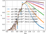
As we mentioned, the Helmholtz equation may be normalized to . The 0th order coefficient is then
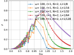
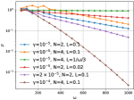
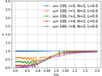
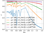
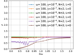
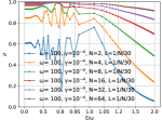
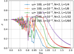
and, with no approximation, the ratio of the imaginary part to the real part is . Fig. 5
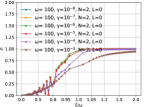
shows the scaling of the convergence factor with . Note that here is the same as the no damping case in Sect. 2.1, so is not shown here. But compared to Fig. 3 with the small dampings , , almost coincide with the no damping case, while roughly mimics .
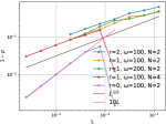
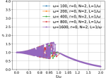
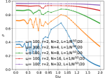
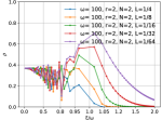
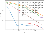
However, this does not imply that the viscoelastic damping in is the same as the first order damping in : the latter has the imaginary/real ratio . So we can expect the two types of damping to differ significantly with large . This is clearly visible in the first line of Fig. 6
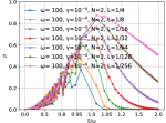
which is drastically different from the first line in Fig. 4. The scaling with number of subdomains is shown in Fig. 6 (middle). For moderate wavenumber, sufficiently small overlap is still required for convergence on many subdomains. There is an optimal overlap width for given , and , which is not investigated here. But with the ad hoc choice of we get the typical scaling for one-level parallel Schwarz methods applied to Laplace problems.
3 Cavity Problem
In the closed cavity problem, on all the boundary. For wellposedness of the problem without damping, we assume the squared wavenumber is not an eigenvalue of the negative Laplace operator.
3.1 Helmholtz operator in the cavity
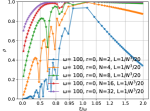
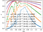
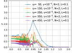
The influence of the first order damping coefficient is shown in Fig. 7.
Compared to Fig. 3 for the waveguide problem, here for the cavity problem the low space frequency has a larger convergence factor. But this difference quickly diminishes as increases, and the scaling for large remains the same, so even the very hard closed cavity problem becomes easy with first order damping.
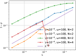
We show in Fig. 8
the corresponding dependence on the other parameters. We see that without first order damping the Schwarz method for the closed cavity problem can not converge at all; see Fig. 8 (top left). With first order damping, convergence is robust in for two subdomains as in the wave guide case, and deteriorates similarly for more subdomains. From the green line (, , ), we can see that, as gradually increases, the convergence here is first slower than, and then close to, the convergence in the wave guide case.
3.2 Helmholtz operator in the cavity
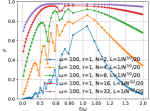
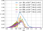
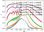
We finally show the influence of the viscous damping coefficient Fig. 9.
We see that similarly to the first order damping, the behavior of the very hard closed cavity case becomes comparable to the wave guide case, especially at , though, at smaller , the convergence at the space low frequency is slower than that in the wave guide. The corresponding dependence on the other parameters is shown in Fig. 10.

References
- (1) Cocquet, P.H., Gander, M.J.: How large a shift is needed in the shifted Helmholtz preconditioner for its effective inversion by multigrid? SIAM Journal on Scientific Computing 39(2), A438–A478 (2017)
- (2) Ernst, O.G., Gander, M.J.: Why it is difficult to solve Helmholtz problems with classical iterative methods. Numerical analysis of multiscale problems pp. 325–363 (2011)
- (3) Gander, M.J., Graham, I.G., Spence, E.A.: Applying GMRES to the Helmholtz equation with shifted Laplacian preconditioning: what is the largest shift for which wavenumber-independent convergence is guaranteed? Numerische Mathematik 131(3), 567–614 (2015)
- (4) Gander, M.J., Zhang, H.: A class of iterative solvers for the Helmholtz equation: Factorizations, sweeping preconditioners, source transfer, single layer potentials, polarized traces, and optimized Schwarz methods. Siam Review 61(1), 3–76 (2019)
- (5) Gander, M.J., Zhang, H.: Schwarz methods by domain truncation. Acta Numerica 31, 1–134 (2022)
- (6) Van Gijzen, M.B., Erlangga, Y.A., Vuik, C.: Spectral analysis of the discrete Helmholtz operator preconditioned with a shifted laplacian. SIAM Journal on Scientific Computing 29(5), 1942–1958 (2007)