Nonresonant quantum dynamics of a relativistic electron in counterpropagating laser beams
Abstract
The quantum dynamics of an ultrarelativistic electron in strong counterpropagating laser beams is investigated. In contrast to the stimulated Compton scattering regime, we consider the case when in the electron rest frame the frequency of the counterpropagating wave greatly exceeds that of the copropagating one. Taking advantage of the corresponding approximation recently developed by the authors for treating the classical dynamics in this setup, we solve the Klein-Gordon and Dirac equations in the quasiclassical approximation in the Wentzel-Kramers-Brillouin (WKB) framework. The obtained wave function for the Dirac equation shows entanglement between the kinetic momentum and spin of the electron, while the spin-averaged momentum coincides with the classical counterpart as expected. The derived wave functions will enable the calculation of the probabilities of nonlinear QED processes in this counterpropagating fields configuration.
I Introduction
Owing to the rapidly developing laser technology, ultraintense coherent laser beams with intensity up to W/cm2 can be generated [1, 2, 3, 4, 5], corresponding to the normalized field amplitude , where , are the electron charge and mass respectively, and the laser vector potential. Relativistic units with are used throughout. Since , the electron dynamics in the presence of the field is highly nonlinear and involve multiphoton emission and absorption. For ultrarelativistic electrons quantum effects in radiative processes are important when the field amplitude experienced in its rest frame approaches the Schwinger field [6]. The ratio between these quantities is known as the quantum strong field parameter , where is the electromagnetic tensor and the particle 4-momentum. It determines the physical regime of the interaction. The motion and radiation of a particle characterized by low value are described by the classical electrodynamics [7]. In the opposite case, however, the recoil caused by a single photon emission is significant, introducing quantum effect to the dynamics. This phenomenon was recently reported [8, 9] and is expected to become dominant in the experiments for next generation laser facilities [10, 11].
The appropriate framework to address laser-particle interaction corresponding to high values is the strong field QED [12]. Usually the Furry picture is applied [13], describing the strong background field as a classical coherent field, and using the Dirac equation solutions in this field as the basis to the QED perturbation theory. Unfortunately, the Dirac equation cannot be analytically solved in the presence of general background fields. Exact solutions exist only for few simplified configurations [14, 15, 16, 17, 18]. Most of the research in the context of strong field QED is based on the Volkov wave function [14, 6], describing a particle in the presence of a plane wave field. While fully adequate to account for the interaction of electrons with a single laser beam, the Volkov solution cannot be used in the presence of a tightly focused beam, multiple beam configuration, or plasma self-generated fields. The common practice in these cases is to assume that in the presence of strong fields the radiation is determined by the local value of the external field, due to smallness of the radiation formation length in ultrastrong fields with respect to the laser wavelength. This approach, known as the Local Constant Field Approximation (LCFA), is the basis of the PIC-QED codes [19, 20], which are the main tool to explore laser-plasma interaction in the high-intensities regime. Notwithstanding of the success of LCFA approach, several recent works [21, 22, 23, 24] pointed out its limitations and possible violations under certain conditions.
Thus, theoretical investigation of QED processes in the presence of complex field configurations requires alternative approaches beyond LCFA. One way is provided by the semiclassical operator techniques introduced by Schwinger [25], and further significantly developed by Baier and Katkov [26, 27, 28]. The Baier-Katkov method is applicable when the electron dynamics in the background fields is quasiclassical and it allows for the evaluation of quantum radiation with a large quantum recoil at a photon emission. In this approach, the photon emission probability amplitude is expressed in terms of the classical trajectory, which effectively means using the Wentzel-Kramers-Brillouin (WKB) approximation in the leading order for the electron wave function in background field. The Baier-Katkov method thus enables the evaluation of quantum radiation in scenarios where the electron motion is quasiclassical and the electron’s classical trajectory is known. The method’s deficiency is that it is limited to tree-level strong-field QED processes.
To achieve a more comprehensive quantum description of QED processes in strong fields, one can explicitly derive the electron wave function in the background field within the WKB approximation and use it in the Furry picture for the calculation of amplitudes of QED processes. Recently, this approach has been applied to investigate strong-field QED processes in tightly focused laser beams [29, 30, 31].
Tightly focusing laser beam is used in experiments to enhance the field strength for a given laser beam energy. However, the same goal can be achieved in multi-beam configurations. For instance, recently it has been proposed to create the so-called dipole wave [32, 33, 34] using combination of multiple laser beams. The simplest example of a multi-beam configuration is the setup of counterpropagating waves (CPW), which provides a compelling platform for studying QED effects [35, 36, 34, 37, 38] and is particularly conducive to the generation of QED cascades [39, 40].
The dynamics of a particle in CPW field configuration strongly depends on the ratio of the laser frequencies observed in the electron’s average rest frame. When this ratio approaches unity, the system enters a resonant regime, leading to phenomena such as the Kapitza-Dirac effect [41, 42, 43, 44] and stimulated Compton emission [45, 46, 47, 48]. Conversely, when the frequency ratio is significantly greater than one, the electrons dynamics is nonresonant and the emitted radiation has spontaneous character rather than stimulated one, exhibiting entirely different features, as explored in various studies [49, 50, 51]. Note that the CPW configuration can induce dynamical trapping, which is highly sensitive to the nature of the emission process [34, 52].
In this paper an approximate solution to the quantum equation of motion for both scalar particles and fermions in the CPW configuration is derived using the WKB technique. Our starting point is the approximate analytical solution of the classical equations of motion obtained by us in Ref. [51]. For the quantum problem, we discuss the same setup, when in the ultrarelativistic electron rest frame the counterpropagating laser wave frequency significantly exceeds that of the copropagating one, and apply the same additional approximations as in the classical case. In virtue of the classical solution, the classical action is found, which further facilitates the construction of the WKB solution. For the derivation of the time-dependent spinorial part of the wave function an iterative technique is applied. With the derived wave function, several quantum characteristics of the dynamics are analyzed in detail.
The paper is organized as follows. Section. II describes the classical theory: II.1 summarizes the results derived in Ref. [51] regarding the electron’s classical trajectory in CPW and II.2 derives the classical action. The WKB wave function as well as its validity criteria appear in Sec. III. In Sec. IV, the spin dynamics resulting from the novel wave function is demonstrated. Sec. V concludes the main findings the work and gives some outlook for the application of the wave function in future work.
II Classical theory
II.1 Classical trajectory
In this subsection the mathematical formulation of the CPW problem is introduced. The approximate solution of the classical equation of motion for a relativistic electron in the CPW setup and its validity condition, derived in our previous work [51], are summarized. The classical equation of motion for a particle in the presence of an electromagnetic field reads
| (1) |
where is the proper time, is the particle’s 4-momentum and is the electromagnetic field tensor. The vector potential corresponding to the circularly polarized CPW configuration is where
| (2) |
| (3) |
where and . The wave vectors read
| (4) |
The scalars are the fields’ amplitudes. In the following we use their normalized values , and , and are unit vectors.
The key assumption, allowing us to perform the integration over the proper time to solve Eq. (1), is that the particle propagates with relativistic velocity at a small angle with respect to the CPW axis. In mathematical terms, the following conditions should be fulfilled
| (5) | |||||
| (6) | |||||
| (7) |
where . It should be noticed that for the sake of simplicity, these conditions are expressed in terms of the quantities in the frame of reference where the counterpropagating waves have the same frequency, rather than in a Lorentz invariant form. The above expressions depend on the time-averaged 4-momentum , which is specified below. Due to the azimuthal symmetry we assume, without loss of generality, that the transverse momentum lies in the axis.
In this setup, as is shown in [51] the following relation is approximately fulfilled
| (8) |
as well as an analogous one with . The symbol stands for either or . Using (8), the Lorentz equation can be integrated and the momentum takes the form
| (9) |
The phases are given by
| (10) | |||||
| (11) |
Without lose of generality, we have chosen the electron to be copropagating with the laser beam . We derive the trajectory via
| (12) |
which yields for its components
| (13) | |||||
| (14) | |||||
The relation between the asymptotic momentum and the average one, as shown in Ref. [51], depends on the turn-on process of the beams. If the beams are turned on separately, an analytical expression exists for the average momentum. In case beam 1 is turned on first, we have
| (16) |
where
| (17) |
In case the second beam is turned on first, analogous derivation leads to
| (18) |
where
| (19) |
It would prove useful to write down explicitly the Lorentz invariant quantities as
| (20) |
The frequencies are related to the average velocity along axis by and . The effective mass is defined as . In our setup, in Lab-frame the counterpropagating laser waves have the same frequency , and the electron (copropagating with ) is ultrarelativistic, accordingly , with . Using Eq. (20), the restrictions imposed by the conditions (5)-(6) on the average electron propagation angle with respect to the laser beam axis () may be expressed by and .
II.2 The classical action
The classical action is defined [53] as
| (21) |
Employing the final momentum obtained above in Eq. (9), as well as the vector potential of the fields defined in Eqs. (2)-(3) and the approximation Eq. (8), the integration is carried out
| (22) |
where are given in Eqs. (10,11). Our final goal is to use the action to construct the WKB wave function. To this end we need to express it in terms of . For this purpose, we multiply the trajectory obtained in Sec. II by :
| (23) |
Owing to this relation, the action is expressed as
| (24) |
Next, we recall that depend on the proper time through . Hence, in order to obtain one should simply replace by , leading to
| (25) |
One can explicitly verify this action by substituting it into the Hamilton-Jacoby relation [53]
| (26) |
which yields indeed the 4-momentum obtained in the previous subsection.
In the case when one of the fields vanishes, Eq. (25) recovers the familiar electron action in a plane wave laser field [14].
III The WKB wave function
The obtained analytical solution of the classical equations of motion in counterpropagating laser fields can be employed to construct the wave function of the electron in the framework of the WKB approximation.
III.1 Solution of Klein-Gordon equation
In the following, we derive the relativistic electron wave function in WKB approximation, beginning with the spinless case. The wave function of a scalar particle in the CPW field configuration satisfies the Klein-Gordon equation:
| (27) |
We employ the WKB Ansatz [54], expressing the solution as a series in :
| (28) |
As the WKB method is a perturbative approach with respect to , we explicitly incorporate into the equations presented in this section for clarity. We obtain in the leading order () the classical Hamilton-Jacobi equation [53]:
| (29) |
which has an approximate solution given by Eq. (25). The equation for the first order correction () reads
| (30) |
Using Eq. (26), the equation for takes the form
| (31) |
This partial differential equation of first order is solved using the characteristics method [55]. Accordingly, the coordinates are given in terms of the characteristic variable
| (32) |
Comparing with (12) one observes that the characteristic variable is proportional to the proper time . Then, Eq. (31) reads
| (33) |
with the solution
| (34) |
Let us explicitly evaluate the integrand, employing the 4-momentum of Eq. (9)
| (35) |
Integrating over we obtain
| (36) |
Since we wish to express the wave function as a function of rather than , the phases are replaced by , respectively, as discussed in the previous section. Furthermore, one notices that according to our key assumption (7), the exponent’s argument is much smaller than 1, and one may therefore Taylor expand it as
| (37) |
Consequently, the first order WKB solution is obtained
| (38) |
where is the interaction volume and is the free particle normalization factor. The coefficient is determined according to the charge normalization
| (39) |
with the Klein-Gordon 4-current
| (40) |
and at vanishing electromagnetic fields. With Eqs. (38) and (40) one obtains
| (41) |
Then Eq. (39) can be rewritten as
| (42) |
We notice that the oscillatory parts of both and are small as compared to their average value. When multiplying both expressions, the second order terms are discarded. The first order terms are either sine or cosine functions with respect to the spatial coordinates, and therefore their contribution to the integration vanishes. Thus, the normalization coefficient reads
| (43) |
Finally, it should be noted that in the case when one of the laser waves vanishes, , the action reduces to its plane wave value, and the Volkov solution [28] is recovered.
Let us discuss now the validity domain of the solution. One may verify that the WKB approximation presented above is equivalent to neglecting the term after substituting the Ansatz to the equation of motion (27). Hence, in order to estimate its validity regime, let us compare the neglected high-order term
| (44) |
with the first-order one
| (45) |
where . Consequently, the WKB solution is valid as long as the following condition is met
| (46) |
which coincides with the Baier-Katkov semiclassical condition [27].
III.2 Solution of Dirac equation
We now extend our calculations to the case of a fermion in CPW configuration, focusing on solving the Dirac equation
| (47) |
where the slash symbol stands for for a general four-vector . are the Dirac matrices and the wave function is a four-component bispinor. It is convenient to use the quadratic form of the Dirac equation, resembling the Klein-Gordon one discussed above. Applying the operator to Eq. (47) one obtains [28]
| (48) |
where the . The WKB Ansatz reads where is now a spinor. While the equation for remains the same as in the Klein-Gordon case, namely Eq. (29), the equation for the first order in contains an additional term as compared to the scalar version (31)
| (49) |
Using Eq. (2) and (3) and the definition of the field tensor , the spinor part takes the form
| (50) |
where the symbol ’ designates derivative with respect to or , respectively. Employing as before the characteristics method one arrives at
| (51) |
We substitute where was derived in the previous section (36) and obtain
| (52) |
As opposed to the scalar case, the equation above does not admit an exact solution, since the matrices do not commute at different times. A possible analytical approximation to this class of mathematical problems is the Magnus expansion [56, 57]. However, in this particular case a second order Magnus expansion was not satisfactory and high order terms turned out to be very cumbersome. Therefore, we put forward an alternative iterative approach.
We notice that, had Eq. (52) been a scalar one, its solution would simply be . Let us examine the series corresponding to the Taylor expansion of the exponent
| (53) |
with and . One may readily verify that successive terms satisfy the following recursive relation
| (54) |
Inspired by this fact, we seek a solution for the spinor equation (52) in the form of Eqs. (53)-(54). By direct substitution of the Ansatz Eq. (53) into Eq. (52) and assuming Eq. (54) is fulfilled, one obtains that the equation is satisfied up to the residual term
| (55) |
In the following, Eq. (54) is solved, yielding a general expression for . We explicitly demonstrate that each term is smaller then the previous one, so the total sum converges to the equation’s solution.
The first step to be taken is to specify the zeroth-order term. We set it to be where is the field free particle bispinor with the normalization being . This choice ensures that our solution satisfies the initial conditions at . Thus, the redundant unphysical solution associated with the second order Dirac equation is excluded [28]. The first-order term straightforwardly reads
| (56) |
In order to solve for the second-order term, it proves convenient to write down explicitly the first beam vector potential, introduced in (2) as
| (57) |
as well as for the second wave. The polarization 4-vector is . The vector potential’s derivative with respect to is therefore
| (58) |
Since as well as , the following identities hold
| (59) |
and analogous ones for . Since the polarization vector satisfies , one may verify that
| (60) |
The integration is carried out using the key approximation (8), as presented in subsection. II.1. Consequently, the second-order term is given by
| (61) |
Employing (57,58) again in order to express the result in terms of one obtains
| (62) |
One may repeat this procedure to obtain a general expression , for the recursive equation (54)
| (63) |
where the exponentials , and were introduced and the symbol stands for the integer part of the number . The functions appearing in the denominator are defined as follows
| (64) |
and
| (65) |
Let us now identify the small parameter of the above expansion. For this purpose we examine two successive orders, and , taking the form given in Eq. (63). Without a loss of generality, we assume that is even. The denominator for both terms scales as . As a result, the first term of the order differs by an additional factor scaling as from the first term of the order. Analogously, the second term acquires an additional factor scaling as . Next, we consider the and orders, and notice that the multiplying factors flip with respect to the previous case. Hence, the is smaller by a factor of from the order. Namely this quantity is the small parameter corresponding to our expansion. It is always much smaller than according to the validity condition Eq. (7), so a convergence is always achieved.
As in the scalar case, in the absence of one of the beams our solution coincides with the Volkov wave function. For instance, substituting the first two terms in the expansion read
| (66) |
Higher-order terms in the expansion vanish due to . Namely, the expansion is truncated and recovers the spinor part of the Volkov wave function [28]. Notice that in the presence of both beams the expansion cannot be similarly truncated, as . As in the scalar case, we may now write the wave function up to the normalization constant
| (67) |
Since the wave function should be a function of rather than , the phases are replaced by , and as in the scalar case.
III.3 The matrix expansion convergence
In the previous section, approximate solutions to the scalar and spinor wave functions were established. For the scalar case, the wave function can be directly substituted into the original Klein-Gordon equation to verify that it satisfies the equation up to a small term corresponding to the second-order WKB correction, as shown in Eq. (46). In contrast, for the spinor case, direct substitution into the Dirac equation (47) is more cumbersome due to the matrix structure of the equation. However, the spinor solution differs from the scalar case only by an additional spin-dependent term, which satisfies Eq.(52). Consequently, demonstrating the convergence of the spinor solution reduces to verifying that this spin-dependent term converges with respect to Eq.(52). This simplifies the analysis, allowing the convergence properties of the spinor solution to be inferred directly from the behavior of this term and the convergence condition for the scalar case [Eq. (46)].
| n | 1 | 2 | 3 | 4 | 5 |
|---|---|---|---|---|---|
In the following, we verify the solution of Eq.(52) in the form of Eq. (53) order by order to demonstrate convergence. Firstly, we specify the parameters of the laser and particle beams, which should fulfill the following requirements:
-
•
For a significant quantum effect, high laser frequency and amplitudes are favourable. Hence, a Free Electron Laser facility operating in the x-ray regime (XFEL) is the best candidate. The chosen laser frequency is reachable in present XFEL facilities and the amplitudes are higher by about an order of magnitude but might be accessible in the next generation ones.
- •
-
•
The WKB validity criterion, Eq. (46), is fulfilled.
-
•
The electric field amplitudes of the waves, , and , remain below the Schwinger field threshold, ensuring that pair production is suppressed [58].
Table 1 presents the average over time and space of the value of the residual term , as defined in Eq. (55), for several orders of the approximate expansion. The results are normalized to , and indicate a rapid convergence, requiring only a few terms to achieve high accuracy.
Before using the wave function to calculate some physical quantities, let us briefly compare the wave function obtained above with the ones presented in [50, 49]. In [50] an approximate solution for the wave function of spinless particles in counterpropagating waves are derived, as well as its WKB limit. Since the authors assume that the angle between the particle propagation and the beams axis is , there is no overlap between their solution and the one presented here, where this angle is assumed to be very small. Nevertheless, the wave function presented here is more favorable for rate calculation for two reasons. First, the validity condition required in [50] are much more restrictive, see Eqs. (41), (55)-(58) there. Second, their solution is given in terms of an infinite series, rendering the rate calculation very cumbersome. On the other hand, in [49] a particle propagating on the beams axis is considered, and a classical solution and the corresponding WKB wave function are derived. The momentum takes then the form of an elliptic integral. In case Eqs. (5)-(7) are fulfilled, the integrand may be Taylor expanded, reducing to the above given expression Eq. (9) with . However, the nontrivial relation between the asymptotic and the average momentum, derived at the end of subsection II.1 in our paper, is not discussed there. Moreover, their solution cannot be used to rate calculation even if the incoming particle transverse momentum is vanishing. The reason is that in this case the outgoing particle will acquire transverse momentum, thus going beyond the approximation validity. The wave function given here, however, applies also for nonnegligible transverse momentum and therefore is suitable for a rate calculation.
IV Spin dynamics
In this section, we use the previously derived WKB wave function to calculate various physical characteristics and compare them with possible classical counterparts, highlighting the role of the quantum effects.
We start by examining the spin of the electron, as it has no classical counterpart and therefore emphasizes the purely quantum effects of the electron’s dynamics. It can be defined as
| (68) |
It should be mentioned that the expectation value of the spin calculated from a WKB wave function also obeys the familiar Bergmann-Michel-Telegdi (BMT) equation, as was generally proven in Ref. [59]. In the instantaneous rest frame of the electron, the 4-pseudovector spin is expressed as . In many high-energy particle reactions, the helicity (namely, the component of parallel to the momentum ) is of particular interest
| (69) |
In the calculations below, we choose the spin to be initially oriented along the -axis, perpendicular to the initial average velocity of the particle ( axis). This configuration is selected because it maximizes the value of , amplifying the spin’s influence on the particle’s motion.
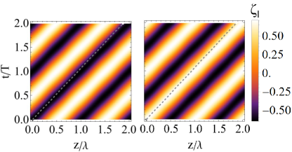
The wave function obtained in the previous section is a function of the 4-vector . Assuming the axis of average motion is , the various phases appearing in the wave function’s expression depend on . Therefore, a better understanding of the spin dynamics arises when one examines the 2D plots (see Fig.1) of the spin as a function of the temporal and spatial coordinates. From the figure we can see that the spin of the electron oscillates in a wide range, . In order to explain the pattern we recall that according to our analytical solution, 3 types of oscillations are to be expected, corresponding to the three phases . The large amplitude ones in the spin arise from the term. For this reason, they take the form of diagonal lines, corresponding to the copropagating beam. The velocity of the electron is smaller than the speed of light, which makes its classical trajectory (gray dashed lines in the figure) lag slowly behind. This fact gives rise to the slow oscillations with frequency [see definition in Eq. (20)], seen also in Fig. 2. The imprint of the second laser pulse is much smaller and is therefore not visible in these plots.
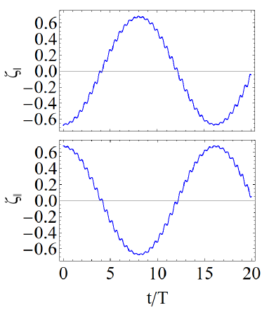
As is well known, in the realm of the WKB approximation, the particle’s free propagation (without taking into account QED processes) approximately follows the classical trajectory . Therefore, we now examine in Fig.2 the spin along the classical trajectory as a function of the laboratory time. Two typical frequencies are observed in the spin dynamics, corresponding those appearing in the classical motion (20). The larger frequency corresponds to the counter-propagating beam through and the small frequency relates to the co-propagating beam through . The ratio between these two frequencies scale as and is enhanced by orders of magnitude for ultrarelativistic particles.
Secondly, let us write down the symmetric stress-energy for the electron
| (70) |
with . The left (right) arrow designates an operator acting to the left (right). The component of this tensor, , is equivalent to the momentum density. Therefore, dividing by the probability density yields the quantum counterpart of the classical momentum, .
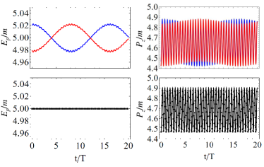
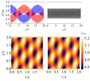
The energy and momentum along the classical trajectory are shown in Fig.3. The black line stands for the spin averaged quantities and the black dots to the classical value. One can observe, as a sanity check, that these two curves coincide, as expected. The spin-dependent quantities exhibit more complex behaviour as compared to the spin-averaged ones. For example, the spin-averaged energy is constant whereas the spin-dependent energy manifests signatures of the frequencies , and discussed above.
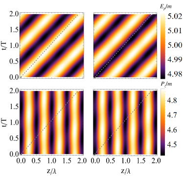
Again, the corresponding 2D plots are presented in Fig 4 to give a broader picture of the dynamics. The energy plot is analogous to the spin component discussed earlier. As for the momentum, the oscillations may be separated to a semi-classical part, originating from the term, and a spin-dependent quantum part, associated with the terms. In Fig 4, the dominant contributions is the semi-classical one, and hence one observes vertical lines (since is time-independent). In case is increased, the quantum part becomes more manifest as can to be seen in Fig 5. Namely, the spin-dependent oscillations are enhanced (right column) and the pattern in the 2D plot is modified accordingly (left column). Such high values of the frequency () are not currently feasible but are useful in order to demonstrate the interplay between the two contributions .
V Discussion and conclusions
In this paper, the quantum dynamics of a scalar/fermion particle in the CPW setup is explored. Assuming the particle is moving with relativistic velocity and a small angle with respect to the CPW axis, the frequency of the co- and counter-propagating beams in the particle’s frame significantly differ from each other. As a result, the system is far from resonance and the Lorentz equation can be approximately integrated analytically. With the aid of the classical trajectory, the Hamilton-Jacoby equation for the classical action is integrated as well. This equation also corresponds to the zeroth-order term of the WKB expansion. Afterwards, the equation describing the first-order WKB term was addressed utilizing the characteristics method. For the scalar case, the integration is exact. For the spinor case, this equation does not admit an exact solution, since the ODE coefficients are matrices rather than c-numbers and therefore do not generally commute with themselves for different times. A unique expansion was used, whose terms are related to each other recursively through a set of ODE’s. Fortunately, given the assumption required in the realm of our classical solution approximation, this set of equations is solved, allowing one to write down general expression for the expansion terms and show their amplitude is decreasing. The validity condition was discussed by evaluating the order of magnitude of the neglected term in the equation. The bottom line coincides with the estimation of Baier and Katkov. Accordingly, the semiclassical approach is adequate as long as the particle energy greatly exceeds the typical frequency of the particle’s motion induced by the external field.
The final result of the derivation, namely the particle’s wave function, paves the way to various research possibilities related to the quantum dynamics of a particle in the presence of a CPW background. For instance, it may be applied to calculate the Schwinger pair production rate for a standing wave. It is well known that this QED process takes place only for electromagnetic configuration with . The simplest way to realize it in the laboratory is the CPW configuration. At present, however, analytical research of this topic is restricted to the pure electric field configuration [60]. It should be mentioned that since our wave function is valid for certain momentum values, only part of the phase space may be reachable. Nevertheless, it can still be valuable for physical insights as well as for benchmarks with extensive numerical models such as the Wigner formalism [61, 62].
Furthermore, this wave function is suitable for calculations of strong-Field QED scatterings, such as nonlinear Compton and Breit-Wheeler (first-order processes) as well as higher order ones (e.g. trident process, mass correction etc). The higher order processes were out of reach until now in the absence of an appropriate wave function. the first order processes may be also obtained within the Baier-Katkov formalism (see for instance [51] regarding the non-linear Compton in CPW), and a detailed comparison would be of fundamental interest. Another intriguing perspective the above presented solution is the spin dynamics of the particle in CPW configuration.
Acknowledgement
QZL and ER contributed equally to the work, to numerical and analytical calculations, respectively. The authors are grateful to K.Z. Hatsagortsyan and C.H. Keitel for their support and valuable comments. ER wishes to thank A. Zigler for fruitful discussions.
References
- Yoon et al. [2021] J. W. Yoon, Y. G. Kim, I. W. Choi, J. H. Sung, H. W. Lee, S. K. Lee, C. H. Nam, J. H. Sung, H. W. Lee, S. K. Lee, S. K. Lee, S. K. Lee, C. H. Nam, C. H. Nam, and C. H. Nam, Realization of laser intensity over w/cm2, Optica 8, 630 (2021).
- Danson et al. [2019] C. N. Danson, C. Haefner, J. Bromage, T. Butcher, J.-C. F. Chanteloup, E. A. Chowdhury, A. Galvanauskas, L. A. Gizzi, J. Hein, D. I. Hillier, N. W. Hopps, Y. Kato, E. A. Khazanov, R. Kodama, G. Korn, R. Li, Y. Li, J. Limpert, J. Ma, C. H. Nam, D. Neely, D. Papadopoulos, R. R. Penman, L. Qian, J. J. Rocca, A. A. Shaykin, C. W. Siders, C. Spindloe, S. Szatmári, R. M. G. M. Trines, J. Zhu, P. Zhu, and J. D. Zuegel, Petawatt and exawatt class lasers worldwide, High Power Laser Science and Engineering 7, e54 (2019).
- Radier et al. [2022] C. Radier, O. Chalus, M. Charbonneau, S. Thambirajah, G. Deschamps, S. David, J. Barbe, E. Etter, G. Matras, S. Ricaud, V. Leroux, C. Richard, F. Lureau, A. Baleanu, R. Banici, A. Gradinariu, C. Caldararu, C. Capiteanu, A. Naziru, B. Diaconescu, V. Iancu, R. Dabu, D. Ursescu, I. Dancus, C. A. Ur, K. A. Tanaka, and N. V. Zamfir, 10 PW peak power femtosecond laser pulses at ELI-NP, High Power Laser Science and Engineering , 1 (2022).
- Li et al. [2022] A. X. Li, C. Y. Qin, H. Zhang, S. Li, L. L. Fan, Q. S. Wang, T. J. Xu, N. W. Wang, L. H. Yu, Y. Xu, Y. Q. Liu, C. Wang, X. L. Wang, Z. X. Zhang, X. Y. Liu, P. L. Bai, Z. B. Gan, X. B. Zhang, X. B. Wang, C. Fan, Y. J. Sun, Y. H. Tang, B. Yao, X. Y. Liang, Y. X. Leng, B. F. Shen, L. L. Ji, R. X. Li, and Z. Z. Xu, Acceleration of 60 MeV proton beams in the commissioning experiment of the SULF-10 PW laser, High Power Laser Science and Engineering 10, e26 (2022).
- [5] The Vulcan facility, https://www.clf.stfc.ac.uk/Pages/Vulcan-laser.aspx.
- Ritus [1985] V. I. Ritus, Quantum effects of the interaction of elementary particles with an intense electromagnetic field, J. Sov. Laser Res. 6, 497 (1985).
- Jackson [1975] J. D. Jackson, Classical Electrodynamics (Wiley, New York, 1975).
- Cole et al. [2018] J. M. Cole, K. T. Behm, E. Gerstmayr, T. G. Blackburn, J. C. Wood, C. D. Baird, M. J. Duff, C. Harvey, A. Ilderton, A. S. Joglekar, K. Krushelnick, S. Kuschel, M. Marklund, P. McKenna, C. D. Murphy, K. Poder, C. P. Ridgers, G. M. Samarin, G. Sarri, D. R. Symes, A. G. R. Thomas, J. Warwick, M. Zepf, Z. Najmudin, and S. P. D. Mangles, Experimental evidence of radiation reaction in the collision of a high-intensity laser pulse with a laser-wakefield accelerated electron beam, Phys. Rev. X 8, 011020 (2018).
- Poder et al. [2018] K. Poder, M. Tamburini, G. Sarri, A. Di Piazza, S. Kuschel, C. D. Baird, K. Behm, S. Bohlen, J. M. Cole, D. J. Corvan, M. Duff, E. Gerstmayr, C. H. Keitel, K. Krushelnick, S. P. D. Mangles, P. McKenna, C. D. Murphy, Z. Najmudin, C. P. Ridgers, G. M. Samarin, D. R. Symes, A. G. R. Thomas, J. Warwick, and M. Zepf, Experimental signatures of the quantum nature of radiation reaction in the field of an ultraintense laser, Phys. Rev. X 8, 031004 (2018).
- The Extreme Light Infrastructure () [ELI] The Extreme Light Infrastructure (ELI), http://www.eli-laser.eu/.
- Exawatt Center for Extreme Light Stidies () [XCELS] Exawatt Center for Extreme Light Stidies (XCELS), http://www.xcels.iapras.ru/.
- Di Piazza et al. [2012] A. Di Piazza, C. Müller, K. Z. Hatsagortsyan, and C. H. Keitel, Extremely high-intensity laser interactions with fundamental quantum systems, Rev. Mod. Phys. 84, 1177 (2012).
- Furry [1951] W. H. Furry, On bound states and scattering in positron theory, Phys. Rev. 81, 115 (1951).
- Wolkow [1935] D. M. Wolkow, Über eine Klasse von Lösungen der Diracschen Gleichung, Z. Phys. 94, 250 (1935).
- Klepikov [1954] N. Klepikov, Zh. Eskp. Teor. Fiz. 26, 19 (1954).
- Sokolov and Ternov [1986] A. A. Sokolov and I. M. Ternov, Radiation from Relativistic Electrons (American Institute of Physics, New York, 1986).
- Redmond [1965] P. J. Redmond, Solution of the Klein-Gordon and Dirac equations for a particle with a plane electromagnetic wave and a parallel magnetic field, J. Math. Phys. 6, 1163 (1965).
- Nikishov [1971] A. Nikishov, Quantum processes in a constant electric field, Sov. Phys. JETP 32, 690 (1971).
- Elkina et al. [2011] N. V. Elkina, A. M. Fedotov, I. Y. Kostyukov, M. V. Legkov, N. B. Narozhny, E. N. Nerush, and H. Ruhl, Qed cascades induced by circularly polarized laser fields, Phys. Rev. ST Accel. Beams 14, 054401 (2011).
- Gonoskov et al. [2015] A. Gonoskov, S. Bastrakov, E. Efimenko, A. Ilderton, M. Marklund, I. Meyerov, A. Muraviev, A. Sergeev, I. Surmin, and E. Wallin, Extended particle-in-cell schemes for physics in ultrastrong laser fields: Review and developments, Phys. Rev. E 92, 023305 (2015).
- Di Piazza et al. [2018] A. Di Piazza, M. Tamburini, S. Meuren, and C. H. Keitel, Implementing nonlinear Compton scattering beyond the local-constant-field approximation, Phys. Rev. A 98, 012134 (2018).
- Di Piazza et al. [2019] A. Di Piazza, M. Tamburini, S. Meuren, and C. H. Keitel, Improved local-constant-field approximation for strong-field QED codes, Phys. Rev. A 99, 022125 (2019).
- Raicher et al. [2019] E. Raicher, S. Eliezer, C. H. Keitel, and K. Z. Hatsagortsyan, Semiclassical limitations for photon emission in strong external fields, Physical Review A 99, 052513 (2019).
- Lv et al. [2021a] Q. Z. Lv, E. Raicher, C. H. Keitel, and K. Z. Hatsagortsyan, Anomalous violation of the local crossed field approximation in colliding laser beams, Physical Review Research 3, 013214 (2021a).
- Schwinger [1954] J. Schwinger, The Quantum Correction in the Radiation By Energetic Accelerated Electrons, Proceedings of the National Academy of Sciences 40, 132 (1954).
- Baier and Katkov [1968] V. N. Baier and V. M. Katkov, Processes involved in the motion of high energy particles in a magnetic field, Sov. Phys. JETP 26, 854 (1968).
- Baier et al. [1994] V. N. Baier, V. M. Katkov, and V. M. Strakhovenko, Electromagnetic Processes at High Energies in Oriented Single Crystals (World Scientific, Singapore, 1994).
- Berestetskii et al. [1982] V. B. Berestetskii, , E. M. Lifshitz, and L. P. Pitevskii, Quantum electrodynamics (Pergamon, Oxford, 1982) chapt.90.
- Di Piazza [2015] A. Di Piazza, Analytical tools for investigating strong-field qed processes in tightly focused laser fields, Phys. Rev. A 91, 042118 (2015).
- Di Piazza [2016] A. Di Piazza, Nonlinear breit-wheeler pair production in a tightly focused laser beam, Phys. Rev. Lett. 117, 213201 (2016).
- Di Piazza [2017] A. Di Piazza, First-order strong-field qed processes in a tightly focused laser beam, Phys. Rev. A 95, 032121 (2017).
- Bulanov et al. [2010a] S. S. Bulanov, V. D. Mur, N. B. Narozhny, J. Nees, and V. S. Popov, Multiple colliding electromagnetic pulses: A way to lower the threshold of pair production from vacuum, Phys. Rev. Lett. 104, 220404 (2010a).
- Gonoskov et al. [2013] A. Gonoskov, I. Gonoskov, C. Harvey, A. Ilderton, A. Kim, M. Marklund, G. Mourou, and A. Sergeev, Probing nonperturbative qed with optimally focused laser pulses, Phys. Rev. Lett. 111, 060404 (2013).
- Gonoskov et al. [2014] A. Gonoskov, A. Bashinov, I. Gonoskov, C. Harvey, A. Ilderton, A. Kim, M. Marklund, G. Mourou, and A. Sergeev, Anomalous radiative trapping in laser fields of extreme intensity, Phys. Rev. Lett. 113, 014801 (2014).
- Kirk et al. [2009] J. G. Kirk, A. R. Bell, and I. Arka, Pair production in counter-propagating laser beams, Plasma Phys. Contr. F. 51, 085008 (2009).
- Bulanov et al. [2010b] S. S. Bulanov, T. Z. Esirkepov, A. G. R. Thomas, J. K. Koga, and S. V. Bulanov, Schwinger limit attainability with extreme power lasers, Phys. Rev. Lett. 105, 220407 (2010b).
- Gong et al. [2017] Z. Gong, R. H. Hu, Y. R. Shou, B. Qiao, C. E. Chen, X. T. He, S. S. Bulanov, T. Z. Esirkepov, S. V. Bulanov, and X. Q. Yan, High-efficiency -ray flash generation via multiple-laser scattering in ponderomotive potential well, Phys. Rev. E 95, 013210 (2017).
- Grismayer et al. [2017] T. Grismayer, M. Vranic, J. L. Martins, R. A. Fonseca, and L. O. Silva, Seeded qed cascades in counterpropagating laser pulses, Phys. Rev. E 95, 023210 (2017).
- Grismayer et al. [2016] T. Grismayer, M. Vranic, J. L. Martins, R. A. Fonseca, and L. O. Silva, Laser absorption via quantum electrodynamics cascades in counter propagating laser pulses, Phys. Plasmas 23, 056706 (2016).
- Jirka et al. [2016] M. Jirka, O. Klimo, S. V. Bulanov, T. Z. Esirkepov, E. Gelfer, S. S. Bulanov, S. Weber, and G. Korn, Electron dynamics and and production by colliding laser pulses, Phys. Rev. E 93, 023207 (2016).
- Kapitza and Dirac [1933] P. L. Kapitza and P. A. M. Dirac, The reflection of electrons from standing light waves, Math. Proc. Cambr. Phil. Soc. 29, 297–300 (1933).
- Batelaan [2007] H. Batelaan, Colloquium: Illuminating the kapitza-dirac effect with electron matter optics, Rev. Mod. Phys. 79, 929 (2007).
- Ahrens et al. [2012] S. Ahrens, H. Bauke, C. H. Keitel, and C. Müller, Spin dynamics in the kapitza-dirac effect, Phys. Rev. Lett. 109, 043601 (2012).
- Dellweg and Müller [2017] M. M. Dellweg and C. Müller, Spin-polarizing interferometric beam splitter for free electrons, Phys. Rev. Lett. 118, 070403 (2017).
- Friedman et al. [1988] A. Friedman, A. Gover, G. Kurizki, S. Ruschin, and A. Yariv, Spontaneous and stimulated emission from quasifree electrons, Rev. Mod. Phys. 60, 471 (1988).
- Pantell et al. [1968] R. Pantell, G. Soncini, and H. Puthoff, Stimulated photon-electron scattering, IEEE J. Quant. El. 4, 905 (1968).
- Fedorov [1981] M. Fedorov, Free-electron lasers and multiphoton free-free transitions, Progress in Quantum Electronics 7, 73 (1981).
- Avetissian [2016] H. K. Avetissian, Relativistic nonlinear electrodynamics (Springer, New York, 2016).
- King and Hu [2016] B. King and H. Hu, Classical and quantum dynamics of a charged scalar particle in a background of two counterpropagating plane waves, Phys. Rev. D 94, 125010 (2016).
- Hu and Huang [2015] H. Hu and J. Huang, Analytical solution for the klein-gordon equation and action function of the solution for the dirac equation in counterpropagating laser waves, Phys. Rev. A 92, 062105 (2015).
- Lv et al. [2021b] Q. Z. Lv, E. Raicher, C. H. Keitel, and K. Z. Hatsagortsyan, Ultrarelativistic electrons in counterpropagating laser beams, New Journal of Physics 23, 065005 (2021b).
- Kirk [2016] J. G. Kirk, Radiative trapping in intense laser beams, Plasma Phys. Cont. Fus. 58, 085005 (2016).
- Landau and Lifshitz [1975] L. D. Landau and E. M. Lifshitz, The Classical Theory of Fields (Elsevier, Oxford, 1975).
- Akhiezer and Berestetskii [1965] A. Akhiezer and V. Berestetskii, Quantum electrodynamics (Interscience, New York, 1965).
- Courant and Hilbert [1989] R. Courant and D. Hilbert, Methods of mathematical physics, vol. 2 (Wiley-VCH, Weinheim, 1989).
- Magnus [1954] W. Magnus, On the exponential solution of differential equations for a linear operator, Communications on pure and applied mathematics 7, 649 (1954).
- Blanes et al. [2009] S. Blanes, F. Casas, J.-A. Oteo, and J. Ros, The magnus expansion and some of its applications, Physics reports 470, 151 (2009).
- Schwinger [1951] J. Schwinger, On gauge invariance and vacuum polarization, Phys. Rev. 82, 664 (1951).
- Rafanelli and Schiller [1964] K. Rafanelli and R. Schiller, Classical Motions of Spin-1/2 Particles, Phys. Rev. 135, B279 (1964).
- Hebenstreit et al. [2009] F. Hebenstreit, R. Alkofer, G. V. Dunne, and H. Gies, Momentum signatures for schwinger pair production in short laser pulses with a subcycle structure, Phys. Rev. Lett. 102, 150404 (2009).
- Bialynicki-Birula et al. [1991] I. Bialynicki-Birula, P. Gornicki, and J. Rafelski, Phase-space structure of the dirac vacuum, Physical Review D 44, 1825 (1991).
- Hebenstreit et al. [2011] F. Hebenstreit, R. Alkofer, and H. Gies, Particle self-bunching in the schwinger effect in spacetime-dependent electric fields, Physical review letters 107, 180403 (2011).