On the Subsidy of Envy-Free Orientations in Graphs111The author names are ordered alphabetically
Abstract
We study a fair division problem in (multi)graphs where agents (vertices) are pairwise connected by items (edges), and each agent is only interested in its incident items. We consider how to allocate items to incident agents in an envy-free manner, i.e., envy-free orientations, while minimizing the overall payment, i.e., subsidy. We first prove that computing an envy-free orientation with the minimum subsidy is NP-hard, even when the graph is simple and the agents have bi-valued additive valuations. We then bound the worst-case subsidy. We prove that for any multigraph (i.e., allowing parallel edges) and monotone valuations where the marginal value of each good is at most $1 for each agent, $1 each (a total subsidy of , where is the number of agents) is sufficient. This is one of the few cases where linear subsidy is known to be necessary and sufficient to guarantee envy-freeness when agents have monotone valuations. When the valuations are additive (while the graph may contain parallel edges) and when the graph is simple (while the valuations may be monotone), we improve the bound to and , respectively. Moreover, these two bounds are tight.
1 Introduction
We study envy-free allocations of indivisible goods, called items in this paper. An allocation is envy-free (EF) if no agent strictly prefers another agent’s bundle [Fol67]. Unlike divisible items where EF allocations always exist [BT95], an EF allocation is not guaranteed to exist when items cannot be divided. Considering a simple example of allocating one item between two agents, both valuing the item at $1, the agent who gets the item would be envied by the other agent. To maintain fairness between the two agents, compensation of $1 can be provided to the agent who receives nothing. More generally, a compelling and pragmatic research problem is to determine the minimal compensation required to ensure EF among agents.
This problem has been widely studied in the literature within the paradigm of fair division with the minimum subsidy. Halpern and Shah [HS19] first proved that when agents have additive valuations and the marginal value of each good is at most 1, a total subsidy of is sufficient to find an allocation so that no agent envies another agent. This result was improved to by Brustle et al. [BDN+20] and this bound is tight as there are instances which require at least subsidy in order to achieve EF. Brustle et al. [BDN+20] also proved that for general monotone valuations an EF allocation always exists with a subsidy of , which was improved to in [KMS+24]. It is worth noting that the tight bound for monotone valuations is still unknown [LLSW24], where the lower bound is . One exception is [BKNS22], in which Barman et al. proved that a subsidy of is necessary and sufficient for monotone valuations with binary marginal values.
We follow the above line of research and restrict our attention to envy-free orientations in graphs – a model that has attracted significant attention since [CFKS23]. Here, agents are the vertices in a graph and goods are the edges so that each agent is only interested in the goods incident to her, which are called relevant items of the agent. An allocation is said to be an orientation if every item is allocated to one of the two incident agents. Christodoulou et al. [CFKS23] introduced this model and proved that deciding the existence of an envy-free up to any item (EFX) orientation is NP-hard. An allocation is EFX if no agent envies another agent’s bundle after (hypothetically) removing any item in it. Zeng and Mehta [ZM24] characterized the structure of the graphs so that it is guaranteed that an EFX orientation exists. Deligkas et al. [DEGK24] strengthened the result of [CFKS23] by proving that even with 8 agents, the problem remains NP-hard when the graph has parallel edges. However, how to use subsidy to compensate agents so that the agents are EF has not been studied before our work.
Therefore, in this work, we address the problem of determining the amount of subsidy required to ensure envy-freeness among agents in the graph orientation problem. Our results span from multigraphs to simple graphs and from monotone valuations to additive valuations. For each setting, we consider the computation problem of finding an EF orientation with the minimum subsidy and the problem of characterizing the corresponding worst-case bound. Our results also partially answer the open problem left in [BDN+20, BKNS22, KMS+24], where for monotone valuations, the upper- and lower-bounds of subsidy are and with the tight bound unknown [LLSW24]. For (multi)graph orientation problem with monotone valuations, we prove that the tight bound of subsidy is .
1.1 Main results
We first consider the computation problem of computing an orientation that achieves EF among agents using the minimum subsidy. We then investigate the worst-case bound of subsidies that can ensure EF in various settings. Regarding the computation problem, we prove that it is NP-hard even for bi-valued additive valuations (see Theorem 2), and is tractable when the valuations are binary additive (see Theorem 4).
| Setting | Upper Bound | Lower Bound |
|---|---|---|
| Multi & Monotone | (Theorem 9) | (Example 20) |
| Multi & Additive | (Theorem 11) | (Example 10) |
| Simple & Monotone | (Theorem 21) | (Example 20) |
We then consider the problem of how much subsidy is sufficient to guarantee envy-freeness. The results are summarized in Table 1. We begin with the most general case where agents have monotone valuation functions and the graph can contain parallel edges (i.e., multigraph). We prove that a subsidy of is sufficient to guarantee EF for all instances. For the lower bound, there exists a simple graph instance where every EF orientation requires a total subsidy of at least . Thus our result is tight up to an additive constant 1, leaving the exact bound as an open problem. It is worth mentioning that this is one of the few cases where linear subsidy is necessary and sufficient to guarantee EF when agents have monotone valuations [BDN+20, BKNS22, KMS+24].
For two special cases, we prove that the results can be improved.
The first improvement, which is the mostly technically involved result in our paper, is for additive valuations, while the graph can still contain parallel edges. Interestingly, for this case, we prove that a subsidy of is necessary and sufficient to ensure an EF orientation. In comparison, without orientation restrictions, the bound of subsidy is . To prove this result, we introduce reserve graphs, where each agent claims exactly one edge in which she has the highest value (called reserve edge of the agent). It is a simple case if no two reserve edges share the same neighborhoods, and we prove that no subsidy is required. When both two agents claim reserve edges from items between them, we prove that a collective subsidy of no more than 1 is sufficient to ensure EF for all agents that these two competing agents can reach in the reserve graph.
The second improvement is for simple graphs, while the valuations are still monotone. Since the lower bound instance for the general case considers simple graphs, a subsidy of is necessary in the worst case. We show that is also sufficient to ensure EF orientations for all simple graphs. To prove this result, we show that when , there is always an envy-freeable allocation such that there are two agents who do not envy other agents before allocating any subsidy.
1.2 Related works
Since EF allocations may not exist, the majority of the literature is focused on its relaxations when subsidy is not allowed. Two widely adopted relaxations are envy-free up to one item (EF1) [Bud11] and envy-free up to any item (EFX) [CKM+19], which requires no agent strictly prefers another agent’s bundle excluding one or any item. EF1 allocations always exist [LMMS04] but the existence of EFX allocations is still unknown except for several special cases, e.g., [PR20, CGM24]. We refer to the recent surveys [AAB+23, LLSW24] for a comprehensive overview of fair allocation. Below we restrict our focus on the graph orientation and fair division with subsidy.
Graph Orientation
Christodoulou et al. [CFKS23] first introduced the graph model where vertices are agents and edges are items such that agents are only interested in their incident items. When agents have additive valuations, they proved that an EFX allocations when the items can be arbitrarily allocated always exists but an EFX orientation where items must be allocated to their incident agents may not exist. Zeng and Mehta [ZM24] identified a family of graphs which admit EFX orientations exist. Kaviani et al. [KSS24] and Deligkas et al. [DEGK24] repectively generalized the graph orientation problem. In the model of Kaviani et al. [KSS24], agents have -bounded valuations, where each item has a non-zero marginal value for at most agents, and any two agents share at most common interested items. They proved that for -bounded valuations, EF2X orientations always exist. In the model of Deligkas et al. [DEGK24], every agent has a predetermined set of items and only receives items from this set. They proved that for monotone valuations, an EF1 allocation always exists. Zhou et al. [ZWLL24] extended the goods model in [CFKS23] to mixed setting when the marginal value of each item can be positive or negative.
Fair Division with Subsidy
Caragiannis and Ioannidis [CI21] first studied the computational complexity of using the minimum amount of subsidies to ensure envy-freeness. Halpern and Shah [HS19] bounded the worst-case amount of subsidies for additive valuations, and Brustle et al. [BDN+20] later improved the result in [HS19]. There is a line of recent works focusing on the variants and generalizations of the standard setting. For example, Goko et al. [GIK+24] considered the strategic behaviors when subsidy is used, and Aziz et al. [AHK+24] considered weighted envy-freeness when the agents have different entitlements. Brustle et al. [BDN+20], Barman et al. [BKNS22] and Kawase et al. [KMS+24] extended the valuations from additive to general monotone, which is also the focus of the current paper. Choo et al. [CLS+24] and Dai et al. [DCW+24] respectively studied the envy-free house allocation with subsidies and its weighted variant. Wu et al. [WZZ23, WZ24] extended the subsidy model to the fair allocation of indivisible chores.
2 Preliminaries
We first introduce the necessary notations and solution concepts in standard fair division problems. Denote by for all . There is a set of items to be allocated to a set of agents. An allocation is an -partition of where refers to the bundle allocated to agent . Each agent has a monotone valuation function such that for any , . Following the convention of the literature on fair division with subsidies, we scale the valuations such that the maximum marginal value of any item is 1. That is . The valuation is additive if for any , . We say item is irrelevant for agent if for all . In other words, the marginal value of assigning an agent her irrelevant item is always 0. Item is relevant for agent if it is not irrelevant.
With no subsidies, an allocation is envy-free (EF) if no agent would prefer the bundles of others to her own bundle, i.e., for any , . Let be the subsidy or payment vector where each agent receives payment . An allocation with payment is envy-free if for any ,
An allocation is said to be envy-freeable (EFable) if there is a payment vector such that is envy-free. It is known that not every allocation is envy-freeable. Halpern and Shah [HS19] characterized all envy-freeable allocations via envy graph. The envy graph for allocation is a complete weighted directed graph with vertices . For any pair of agents , the weight of arc in is , i.e., the envy of agent on agent ’s bundle.
Theorem 1 (Halpern and Shah [HS19]).
Given any allocation , the following statements are equivalent:
-
(a)
is envy-freeable;
-
(b)
maximizes the total value of agents among all reassignments of its bundles to agents, i.e., for every permutation , ;
-
(c)
contains no directed cycle with positive weight.
Graph Orientation
In this work, we assume that agents are vertices in a (multi)graph and items are edges so that the relevant items to an agent are exactly the edges incident to her. Formally, given a graph , we use to denote the set of edges between , where and if are non-adjacent. Let be the set of edges incident to , i.e, ’s relevant items. When the graph is simple, contains at most one edge and we use to denote this edge if . Then for a simple graph. In summary, we have and such that for all . We focus on a restricted type of allocations. An orientation with respect to is an allocation such that . If not explicitly stated otherwise, all allocations in this paper are assumed to be orientations.
Given orientation of , for any , let for simplicity. The orientation is locally envy-freeable with respect to agents if the partial allocation of is envy-freeable, i.e., . The orientation is locally envy-freeable if for every pair of agents , the partial allocation of is envy-freeable.
We without loss of generality assume throughout this paper that the given (multi)graph is connected. If the graph consists of multiple components, we can add new edges until there exists exactly one component. Denote the resulting graph as . Let the agents incident to each new-added edge have value 0 for the edge. Then an EF orientation with payment in can be converted to an EF orientation with payment in ; this can be achieved by arbitrarily distributing the new-added edges to incident agents. The reverse direction is also true. As only the orientation varies, we can claim that there exists an EF orientation of with total subsidy at most a number if and only if there exists an EF orientation of with total subsidy at most .
2.1 Algorithmic Components
In this section, we recall some simple algorithms in resource allocation, which will be used as subroutines in our algorithms. Although these algorithms work for an arbitrary number of agents, it is sufficient for us to focus on the case with two agents.
Round-Robin ()
The algorithm takes a pair of ordered agents and and a set of items . Agents and take turns selecting their favorite remaining item from until all items are allocated. When the two agents have additive valuations, returns an EF1 allocation.
Envy-Cycle Elimination ()
The algorithm takes two agents and and a set of items . In each round, selects the agent that is not envied by the other one to receive one remaining item in until all items are allocated. If there is mutual lack of envy between both agents, arbitrarily select one of them. If both agents envy the other one, first swaps their current allocations before selection. returns an EF1 allocation for monotone valuations.
Maximum Total Utilities ()
For each item in , it is allocated to the agent who has a higher value on it, and ties are broken arbitrarily. The algorithm always maximizes the total value of the two agents but does not necessarily have fairness guarantees.
3 Complexity of Computing Minimum Subsidy
In this section, we present our computational results on the problem of computing an EF orientation with the minimum total subsidy when the valuations are additive. We demonstrate that, perhaps surprisingly, the problem is NP-hard if the edge values are in , but is polynomial-time solvable if edge values are in .
3.1 NP-hardness for Edge Values in
We start with the hardness result. For the ease of presentation, we consider the valuations with for all and . We can simply divide all the values by 2 in order to satisfy the scaled assumption of maximum marginal value being 1.
Theorem 2.
Computing an orientation with the minimum subsidy is the NP-hard, even when the graph is simple and the valuations are additive and for all and .
Proof.
It suffices to prove the NP-completeness of checking whether an EF orientation exists or not. We reduce from the NP-complete problem 2P2N-3SAT [BKS03, Yos05]. A 2P2N-3SAT instance contains a Boolean formula in conjunctive normal form consisting of Boolean variables and clauses . Each variable appears exactly twice as a positive literal and exactly twice as a negative literal in the formula. Each clause contains three distinct literals.
Given a 2P2N-3SAT instance , we construct a graph orientation instance without parallel edges as follows:
-
•
For each variable , create two vertices and one edge with a value of 2 to both and .
-
•
For each clause , create a vertex . If contains a positive literal , then create an edge with value 1 for both incident vertices. If contains a negative literal , then create an edge with value 1 for both incident vertices.
-
•
Create a dummy vertex for every clause , and an edge with a value of 1 for both incident vertices.
In summary, we create a graph orientation instance with vertices and edges. Only the edges of form ’s are valued at 2 by their incident vertices, and all other edges have a value of 1 by their incident vertices. Observe that the degree of each dummy vertex is 1, and thus, in an EF orientation, every vertex must receive edge . We now show that a 2P2N-3SAT instance is satisfiable if and only if there exists an EF orientation.
Suppose the 2P2N-3SAT instance is satisfiable. For each variable that is set to True in the satisfiable assignment, we allocate to . Then, allocate the other two edges incident to to the corresponding clause vertices. For , there are also two edges linking two clause vertices to it, and then allocate these two edges to . Similarly, if is set to False, allocate to . Additionally, allocate the other two edges incident to to their corresponding clauses. For , allocate the edges connecting to the clause vertices to . Finally, for every edge , allocated it to . We have allocated all edges to their incident vertices, it remains to show that this allocation is EF. Each vertex is EF since she receives her unique-valued item. Each receives a value of at least 1 as there exists at least one literal contained in that evaluates to True in the satisfiable assignment. Thus, is also EF. For variable that is set to True, the vertex receives an item with a value of 2, and receives two incident edges linking to clause vertices and has a value of 2. A similar argument shows that when is set to False, both and receive value 2. Therefore, the resulting orientation is indeed EF.
For the reverse direction, suppose that there exists an EF orientation. Construct an assignment of as follows: if is allocated to , then set to True, and otherwise, set to False. The constructed assignment is valid, which means that exactly one of is set to True. We now show that this assignment is satisfiable. Assume, for the sake of contradiction, that there exists a clause that evaluates to False. In this case, the vertices corresponding to the three literals in would not receive the item with value 2. To satisfy EF, each of these vertices must receive the edge linking her to . Consequently, needs to receive to avoid envying the variable vertices adjacent to her. However, this allocation would make envy , which is a contradiction. Therefore, the constructed assignment is a satisfiable assignment. ∎
We remark that the above theorem indicates that it is NP-hard to differentiate between zero subsidy and a positive subsidy. Therefore, there is no polynomial time algorithm with a bounded approximation guarantee for the problem of computing the orientation with the minimum subsidy. Given this, we study the subsidy bounds that always guarantees an EF orientation in Sections 4, 5, and 6.
3.2 Efficient Algorithm for Edge Values in
We next prove that when the valuation functions are additive and binary (i.e., the value of every edge is in ), computing the minimum subsidy orientation can be solved in polynomial time. Starting from , if an edge is valued at 0 by both incident vertices, we remove that edge. Note that the removal of those edges does not affect the required subsidy. With a slight abuse of notation, for the remainder of this section, let denote the graph obtained after removing the above-mentioned edges. If an edge is valued at 1 by both incident vertices, it is called critical. If it is valued at 1 by exactly one of its incident vertices, it is called non-critical.
We now introduce four properties that a component of may satisfy:
-
(P1)
contains a non-critical edge.
-
(P2)
contains a simple cycle222A simple cycle with length in a multigraph is a simple path such that vertices are distinct, and for and . of length at least 3 where every edge is critical.
-
(P3)
contains a pair of adjacent vertices and such that the number of critical edges in is even.
-
(P4)
contains vertices such that there are at least two critical edges in , and at least two critical edges in .
We first prove that a component admits an EF orientation if and only if it satisfies at least one of properties (P1)–(P4).
Lemma 3.
For a component of , there exists an EF orientation of if and only if satisfies at least one of properties (P1)–(P4).
Proof.
For the “if” direction, we prove that Algorithm 1 terminates and returns an EF orientation. Since the input satisfies at least one of the properties (P1)–(P4), first time when the while loop in Line 6 is executed, there exists at least one agent with a positive Label. In the while-loop, during each iteration, we remove one vertex and moreover set the Label of at least one other remaining vertex to a positive integer. Therefore, the while-loop terminates with and all edges are allocated.
Next, we prove the resulting orientation is EF. Observe that when the while loop is executed, we can assume that every edge is critical; otherwise, this would imply that property (P1) is satisfied, and thus every 0-1 edge could have been removed. Note that it suffices to check the EF condition only among neighboring vertices and , since if there are no edges between two different vertices, there cannot be any envy between them.
Let and be arbitrary adjacent vertices. One of these two vertices must have been selected earlier in the while loop (without loss of generality, let this vertex be ). When is selected by the while loop, her value is equal to . Thus, when the vertex is removed in Line 7, her value is at least , ensuring that does not envy . Since the remaining edges are all allocated to agent by Line 8, we also have that does not envy . Thus, any two neighboring vertices are EF toward each other, implying that the outputted orientation is EF, as needed.
We now consider the “only if” direction and prove that if satisfies none of (P1)-(P4), then does not have an EF orientation. For the sake of contradiction, assume that does have an EF orientation. As does not satisfy property (P1), it follows that does not contain non-critical edge; thus, every edge is critical. Denote as the number of edges between any two adjacent vertices .
Consider a directed graph , induced by the EF orientation, with vertex set and edge set defined as
We see that in any EF orientation, each vertex in must have an out-degree at least one. This holds because in : (i) the number of edges between any two vertices is odd, and (ii) for each with at least two neighbors, has at most one neighbor with whom it shares more than one edge. These facts imply that if has out degree zero in , it receives a value of at most , implying that envies one of its neighbors. Thus, indeed the out-degree of each vertex in must be at least one.
A directed graph where each vertex has out-degree at least one must contain a cycle. Hence, we see that must contain a cycle. Furthermore, since if then , we see that the cycle must be of length at least 3. However, a cycle of length at least 3 in implies the existence of a cycle of the same length in , which means that satisfies property (P3), contradicting the assumption that does not satisfy any of the properties (P1)–(P4). Hence, by contradiction, there is no EF orientation of . ∎
We now present the main result of this section.
Theorem 4.
When agents have binary additive valuations, the minimum subsidy required to ensure EF orientation is equal to the number of connected components that do not satisfy any of the properties (P1)–(P4). Furthermore, the EF orientation that achieves this minimum subsidy can be computed in polynomial time.
Proof.
Suppose consists of connected components , , where each satisfies one of the properties (P1)–(P4), while each satisfies none of them. We show that subsidy of , corresponding to one dollar per each component not satisfying (P1)–(P4), is both necessary and sufficient for to have an EF orientation.
By Lemma 3, each component has an EF orientation, and each vertex receives a value of at least 1. Thus for each , if some agent receives a subsidy of at most 1, then is EF towards . Then to establish the subsidy bound in the theorem statement, it suffices to show that for each component not satisfying any of (P1)–(P4), subsidy of 1 is both necessary and sufficient for to have an EF orientation; this guarantees that no envy between vertices from different components.
According to Lemma 3, for the component , there exists no EF orientation, indicating that a positive subsidy is necessary. We then demonstrate that a subsidy of 1 suffices. Select an arbitrary vertex , give a subsidy of 1, and set . Then, proceed directly to the while loop in Algorithm 1. The arguments provided in Lemma 3 imply that the while loop terminates and that the resulting orientation is EF. As only one agent received subsidy 1, we conclude that has an EF orientation with subsidy 1.
Finally, in order to compute the EF orientation of , we essentially run Algorithm 1 on each of the components of , with a minor adjustment for those components that do not satisfy any of the properties (P1)–(P4). Since the running time of Algorithm 1 is , and the number of components of is at most , we see that the EF orientation of with the minimum subsidy can be computed in time . ∎
4 Subsidy Bounds for Monotone Valuations and Multigraphs
In this section, we focus on the general case where the graph contains parallel edges and the valuations are monotone. Suppose that valuations are given as oracle. Our main result is a polynomial-time algorithm that outputs an EF orientation using at most subsidy. As we will see in Section 6 (Example 20), there are instances where every EF orientation requires a subsidy of at least (even when there are no parallel edges), and thus our result in this section is tight up to an additive constant of 1.
Before presenting our algorithm, we first observe that achieving local envy-freeability between every pair of adjacent agents does not imply envy-freeability for the orientation as a whole. We consider the following example.
Example 5.
Consider a complete graph with 3 agents . We first construct , items between agents and , and the corresponding valuations. The set of items is partitioned into two bundles with agents’ valuations: . A local envy-freeable partial allocation is to assign to agent 2 and to agent 1. For the set of items, we also split it into two bundles , and the valuations of agents are . Then allocate to agent 2 and to agent 3 resulting in a locally envy-freeable partial allocation. Similarly, the set of items is partitioned into and , with agents’ valuations being . Similarly, the partial allocation where agent receives and agent receives is locally envy-freeable. Now we get an orientation of where . As for agents’ valuations of their bundles, we define , which does not violates the monotonicity of ’s. However, since in the envy graph , the weight of cycle is 1, the orientation is not EFable by Theorem 1.
We circumvent such technical difficulties and show that, for multigraphs, a total subsidy of is sufficient. We now establish a structural property that will be useful later.
Lemma 6.
The allocation returned by Algorithm 2 does not contain any envy-cycle.
Proof.
Consider a directed graph where every agent corresponds to a vertex and arc from to exists if and only if agent envies in allocation . We now show there is no cycle in . Suppose, for the sake of a contradiction, there exists a cycle in . For notational convenience, let agent be . For any , agent envies , and thus and are adjacent vertices in and . Moreover, by Line 4, when determining the partial allocation of , both agents and prefer the same bundle between and . Suppose that both prefer than the other bundle. Since agent envies in allocation , bundle is permanently allocated to agent ; note in this case, . By Line 4, for any , we have
Summing up and eliminating from both sides,
| (1) |
where is identical to , the bundle permanently allocated to agent 1. Moreover, since is a cycle in , for any , we have
| (2) |
where the equality transition is due to the property of orientation. Combining inequalities (1) and (2), we have
where the first inequality holds because for any , and valuation functions are monotone; the second transition is due to inequality (1); the third inequality transition is due to inequality (2). Thus, by contradiction, there is no cycle in . ∎
Lemma 7.
Algorithm 2 returns an envy-freeable allocation .
We now present the upper bound on the subsidy for each agent. The result of [HS19] states that for any envy-freeable allocation , a valid subsidy payments which ensures envy-free is to set , where is the weight of the maximum weight directed path starting from vertex in the envy graph . For the allocation returned by Algorithm 2, we also set the payments as . We now show that, for the returned allocation, weight of the maximum weight directed path is at most 1, which implies .
Lemma 8.
Let be the maximum weight directed path in the envy graph , where is the allocation returned by Algorithm 2. The weight of is at most 1.
Theorem 9.
For multigraphs with monotone agent valuations, there always exists an EF orientation with a total subsidy of at most , and it can be computed in polynomial time using value queries.
5 Improved Bounds for Additive Valuations
In this section, we improve Theorem 9 for additive valuations, where the graph can still contain parallel edges. As we will see, breaking is far more technically involved. We first present an instance for which we can conclude that a subsidy of is necessary to achieve an EF orientation when valuations are additive.
Example 10.
Consider a simple graph consisting of parallel edges, assuming is even, where each edge is valued at one by both of its endpoint agents. For this instance, a subsidy of is required to achieve an envy-freeable orientation since every edge can be allocated to at most one of the endpoint agents and the other agent needs a subsidy of 1.
One may wonder whether the “Bounded-Subsidy Algorithm” in [BDN+20] can achieve the worst-case bound of , we show the answer is “no” even for simple graphs. The instance is presented in Appendix.
We fist introduce several definitions. Recall that, given graph , is the set of items between . Given an orientation of , for any , refers to with subscript representing that these items in the bundle of agent and with superscript and subscript representing that these items are from . We say an orientation is locally EFable when restricting to or regarding , if and only if . We also use the positive part operator defined as follows: for any ,
The main result of this section is a polynomial time algorithm that computes an EFable orientation requiring a total subsidy of at most for multigraphs.
Theorem 11.
For multigraphs and additive agent valuations, there exists an EF orientation with a subsidy of at most , and it can be computed in polynomial time.
We now introduce the idea of our algorithm. There are two phases: in Phase 1, we allocate items between adjacent agents in the reserve graph (will be introduced below), and in Phase 2, we allocate items between non-adjacent agents in . The , a directed graph, is constructed as follows; Each agent forms a vertex in ; For arcs, let each agent arbitrarily pick an item with and add arc to . Then is formed by connected components .
is essentially a subgraph of where and every agent claims exactly one favorite item incident to her as the edges in . By our normalization, must have value 1 for this item. To indicate the claimant of edges in , we add directions to edges in . If agent claims as the favorite, then the edge goes from to . That is the edges in pointing to their claimants. Note that if there are two adjacent agents and claim the same edge , then there are two directed edges between vertices , one from to and the other one from to .
In Phase 1, we allocate items between adjacent agents in each component . Items between two agents are allocated based on two routines, and . The lets agents , in turn, pick their most preferred one from the remaining items and agent picks first; the order is crucial. The allocates each item to the agent having a larger value for and if there is a tie, allocate that item to agent .
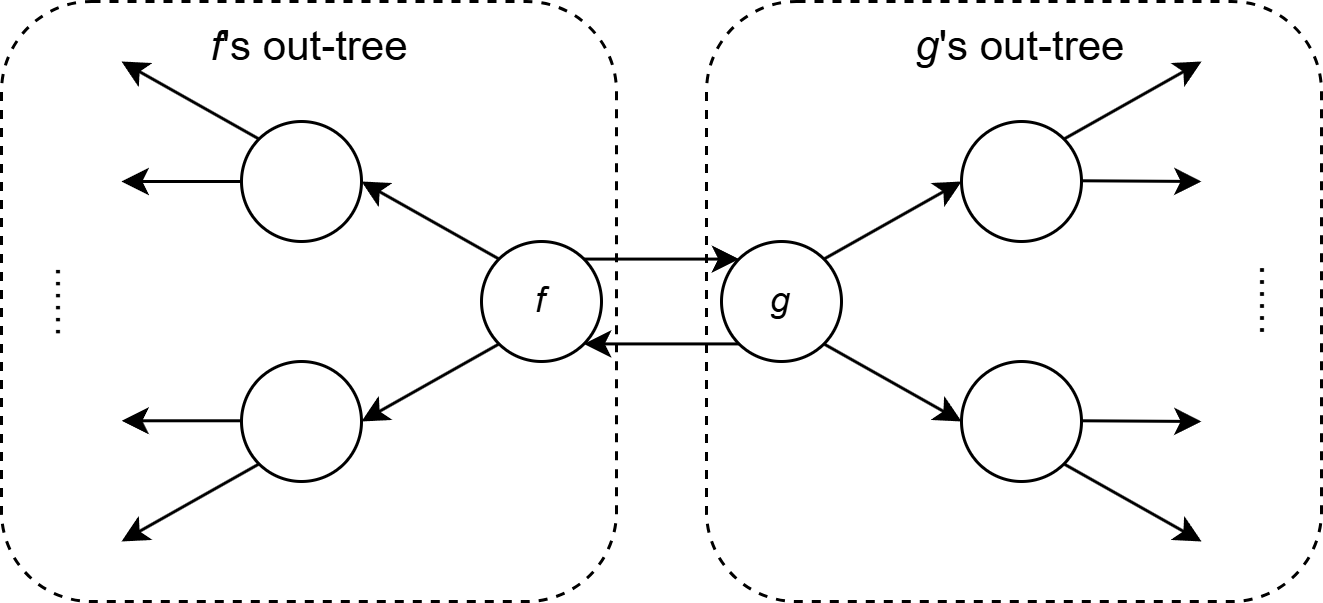
We will distinguish whether component contains a cycle with a length of 3 or more. The case where has such a cycle is relatively easy to handle and we use to allocate items between any pair of adjacent agents in , with a specific picking order determined by . For the other case where has a 2-cycle, composed by vertices , we first form out-trees of and of (see Figure 1 for an illustration) and will proceed with the allocation of each out-tree from the corresponding root to all depth 1 vertices and then from depth 1 vertices to all depth 2 vertices, until to the leaves. Depending on the partial allocation of , we have different allocation rules. If is allocated such that do not envy each other, then we use subroutine to allocate items in both out-trees. For the other case, we use subroutine to allocate the out-tree of the envious agent between while for that of the other. Informally, the is almost identical to . The will classify the successors of the current vertex and implement either or based on the specific classification.
We note that for agent , (Line 4 of ) is determined before allocating the bundle between and ’s out-neighbor while is determined after all items between and ’s out-neighbor are allocated. The high-level idea of is for quantifying the ’s out-neighbor into different ’s and for , it is used to determine for every out-neighbor of . Indeed, as we will see, are the upper bounds of the minimum subsidy of envy-freeable allocations for each agent . Moreover, we remark that both and will be updated at most once.
In Phase 2, we allocate items between agents non-adjacent in . The allocation rule is and we will swap bundles whenever necessary. The formal description of the algorithm is introduced in Algorithm 5. The parameters are used to classify successors in and we remark that they also act as upper bounds of the final payment for agent , which we will prove below.
Before proving the main results, we first present observations and propositions regarding the algorithm and subroutines.
Observation 12.
For every pair of agents and , if they are adjacent in , then bundles and are determined by either or .
This observation directly follows from the way of allocating in the algorithm. We remark that necessary swaps such as Line 33 in and Lines 10 and 23 in Algorithm 5, are made to ensure local EFablility.
Proposition 13.
Suppose , then and hold. If respectively assigning and to agents and does not result in a locally envy-freeable allocation, then .
The proposition indicates that once the allocation of is determined by in the algorithm, the envy of any of these two agents towards the other is at most 1.
Proposition 14.
Suppose and there exists an item valued at 1 by agent , then .
The proposition states that if the allocation of is determined by and the advantage agent has a value of 1 for some item in , then the advantage agent receives a value of at least 1 from items . The following proposition indicates the bounds of and (if applicable).
Proposition 15.
For agent , if the items between and ’s direct successors in the connected component of are allocated by , then in the same component, has a direct predecessor . Moreover, and after updating in Line 38 of , .
Proof.
The fact that has a predecessor in the same component directly follows from Algorithm 5. Since arc exists in , according to Line 2 of Algorithm 5, there exists such that . Thus, holds as is a 2-partition of . Then we have the following,
where the first inequality transition is due to .
For the bound between and , if , then holds trivially. For the case where , we have for some belonging to ; recall that is the set of direct successors of in (excluding , which we must take into account when determining ). If , by the definitions of , we directly have . If , at the moment when computing at Line 38, . By , we have and the following holds,
The first inequality comes from and . For the second one, since , the 2-partition of is determined by , and hence by Proposition 13, . The third one is due to . ∎
In what follows, we present a crucial lemma, helpful for bounding the total required subsidy. stating that for some agent , if is used to allocate items between and ’s direct successors in some component of , then . Note that if ’s predecessor is also her successor, we always exclude the predecessor from .
Lemma 16.
If is used to allocate items between and ’s direct successors in a component of , then .
To prove this lemma, we establish the key properties guaranteed by for ’s direct successors. The proof of this lemma involves a detailed discussion and is deferred to Appendix.
Lemma 17.
For each component in , let be the set of vertices in . Then it holds that at termination of Algorithm 5.
Proof of Lemma 17.
First, we remark that ’s do not get updated on or after Line 22 of Algorithm 5. The algorithm only updates ’s in and hence if for some , then is used to allocate the items adjacent to agents in , Let be the root of the out-tree. Then according to Proposition 15, for any in the rooted tree of , holds. Then by applying Lemma 16 from the leaves to the direct successors of root , we have
where the last two inequality transitions follow from Lemma 16. Note that in the proof of Lemma 16, we have proved when is the root and therefore complete the proof of the lemma. ∎
At the end of Algorithm 5, we will let each agent receive bundle and payment . According to Phase 2 of Algorithm 5, for any , holds. Thus, the total subsidy where the last inequality follows from Lemma 17 and the fact that every component has at least two vertices. Hence, the remaining is to prove that the orientation with payment is envy-free.
Lemma 18.
At the moment right before Phase 2, no agent envies their out- and in-neighbours in if is the payment to agent .
Lemma 19.
At the termination of Algorithm 5, the allocation with payment is envy-free.
The proofs for the above two lemmas involve detailed analysis of for all . The formal proofs can be found in the appendix.
6 Improved Bounds for Simple Graphs
Finally, we improve Theorem 9 for simple graphs, where the valuations can be arbitrarily monotone. We start with the lower bound.
Lower bound.
The following example gives an instance for which any EF orientation requires a subsidy of at least .
Example 20.
Consider a simple graph with two connected components and , where:
-
•
is a single edge connecting two vertices denoted , and both agents (vertices 1 and 2) value the edge incident to them at 1.
-
•
is a complete graph with . The value of each agent depends solely on the number of edges they receive, and is given by the valuation
In any orientation of , one agent (say agent 1) receives the edge, leaving the other agent (agent 2) with value zero. To ensure an EF orientation, agent 2 must receive a subsidy of 1. For every agent , their value is 0 unless they receive all the edges incident to them. Therefore, in any orientation, at most one agent in can achieve a value of 1, while the others receive zero. Since agent 2 from receives a subsidy of 1, the agents in who have zero value (there are of them) must each receive a subsidy of 1 to maintain EF. Thus, the minimum subsidy needed for an EF orientation in this instance is .
Upper bound.
We now show that a subsidy of is sufficient to guarantee EF. At a high level, we find an EF orientation for which at least two agents receive zero subsidy. The choice of such agents depends on both the structure of and the agents’ valuations.
Theorem 21.
For simple graphs with monotone agent valuations, there always exists an EF orientation with a subsidy of at most , and it can be computed in polynomial time using value queries.
Proof.
We show that Algorithm 6 returns an EF orientation with total subsidy of at most . As the maximum marginal value of each edge is at most 1, we see that .
Consider any pair of agents . We show that is EF towards . Note that the claim holds immediately when and are not adjacent or the edge is oriented toward , since . Thus, we may only focus on the case where and are adjacent and the edge is oriented towards . If , we have . Furthermore, if , meaning that , we have
where the second inequality follows from , which follows from the fact that and Line 3 was executed.
Next, we show that no agent envies , and that is EF towards any other agent. Since receives all the edges incident to her, we have for any , which means that does not envy any other agent. Furthermore, for any , we have , noting , we have that any agent does not envy . Hence, is indeed EF.
As for the subsidy bound, we now show that at least one other vertex other than receives a subsidy of zero. Recall that , and . Since , one of two agents, say , receives the edge , and thus has value at least (by Line 3), meaning that they get zero subsidy. Therefore, at least two agents ( and ) receive zero subsidy, and since for each , the total subsidy is at most .
Finally, we observe that Algorithm 6 runs in time and makes at most value queries. ∎
7 Conclusion
In this paper, we provide the (tight) bounds of the minimum subsidy to compensate agents in order to achieve an envy-free allocation in the graph orientation problem. Our paper uncovers several interesting problems for subsequent research. Firstly, there is a constant additive gap between the upper and lower bounds in the general case of multigraph and monotone valuations. Closing this gap is an intriguing theoretical problem. Secondly, we have been focusing on the allocation of goods and the mirror problem of chores/mixed manna has not been studied yet. Finally, the optimal bound of subsidy in the unrestricted setting (outside the scope of graph orientations) when agents have arbitrary monotone valuations [BDN+20, BKNS22, KMS+24] remains unknown.
References
- [AAB+23] Georgios Amanatidis, Haris Aziz, Georgios Birmpas, Aris Filos-Ratsikas, Bo Li, Hervé Moulin, Alexandros A. Voudouris, and Xiaowei Wu. Fair division of indivisible goods: Recent progress and open questions. Artif. Intell., 322:103965, 2023.
- [AHK+24] Haris Aziz, Xin Huang, Kei Kimura, Indrajit Saha, Zhaohong Sun, Mashbat Suzuki, and Makoto Yokoo. Weighted envy-free allocation with subsidy. CoRR, abs/2408.08711, 2024.
- [BDN+20] Johannes Brustle, Jack Dippel, Vishnu V. Narayan, Mashbat Suzuki, and Adrian Vetta. One dollar each eliminates envy. In EC, pages 23–39. ACM, 2020.
- [BKNS22] Siddharth Barman, Anand Krishna, Yadati Narahari, and Soumyarup Sadhukhan. Achieving envy-freeness with limited subsidies under dichotomous valuations. In IJCAI, pages 60–66. ijcai.org, 2022.
- [BKS03] Piotr Berman, Marek Karpinski, and Alex D. Scott. Approximation hardness of short symmetric instances of MAX-3SAT. Electron. Colloquium Comput. Complex., TR03-049, 2003.
- [BT95] Steven J Brams and Alan D Taylor. An envy-free cake division protocol. The American Mathematical Monthly, 102(1):9–18, 1995.
- [Bud11] Eric Budish. The combinatorial assignment problem: Approximate competitive equilibrium from equal incomes. Journal of Political Economy, 119(6):1061–1103, 2011.
- [CFKS23] George Christodoulou, Amos Fiat, Elias Koutsoupias, and Alkmini Sgouritsa. Fair allocation in graphs. In EC, pages 473–488. ACM, 2023.
- [CGM24] Bhaskar Ray Chaudhury, Jugal Garg, and Kurt Mehlhorn. EFX exists for three agents. J. ACM, 71(1):4:1–4:27, 2024.
- [CI21] Ioannis Caragiannis and Stavros Ioannidis. Computing envy-freeable allocations with limited subsidies. In WINE, volume 13112 of Lecture Notes in Computer Science, pages 522–539. Springer, 2021.
- [CKM+19] Ioannis Caragiannis, David Kurokawa, Hervé Moulin, Ariel D. Procaccia, Nisarg Shah, and Junxing Wang. The unreasonable fairness of maximum nash welfare. ACM Trans. Economics and Comput., 7(3):12:1–12:32, 2019.
- [CLS+24] Davin Choo, Yan Hao Ling, Warut Suksompong, Nicholas Teh, and Jian Zhang. Envy-free house allocation with minimum subsidy. Oper. Res. Lett., 54:107103, 2024.
- [DCW+24] Sijia Dai, Yankai Chen, Xiaowei Wu, Yicheng Xu, and Yong Zhang. Weighted envy-freeness in house allocation. CoRR, abs/2408.12523, 2024.
- [DEGK24] Argyrios Deligkas, Eduard Eiben, Tiger-Lily Goldsmith, and Viktoriia Korchemna. Ef1 and efx orientations, 2024.
- [Fol67] Duncan Foley. Resource allocation and the public sector. Yale Economic Essays, pages 45–98, 1967.
- [GIK+24] Hiromichi Goko, Ayumi Igarashi, Yasushi Kawase, Kazuhisa Makino, Hanna Sumita, Akihisa Tamura, Yu Yokoi, and Makoto Yokoo. A fair and truthful mechanism with limited subsidy. Games Econ. Behav., 144:49–70, 2024.
- [HS19] Daniel Halpern and Nisarg Shah. Fair division with subsidy. In SAGT, volume 11801 of Lecture Notes in Computer Science, pages 374–389. Springer, 2019.
- [KMS+24] Yasushi Kawase, Kazuhisa Makino, Hanna Sumita, Akihisa Tamura, and Makoto Yokoo. Towards optimal subsidy bounds for envy-freeable allocations. In AAAI, pages 9824–9831. AAAI Press, 2024.
- [KSS24] Alireza Kaviani, Masoud Seddighin, and AmirMohammad Shahrezaei. Almost envy-free allocation of indivisible goods: A tale of two valuations. CoRR, abs/2407.05139, 2024.
- [LLSW24] Shengxin Liu, Xinhang Lu, Mashbat Suzuki, and Toby Walsh. Mixed fair division: A survey. J. Artif. Intell. Res., 80:1373–1406, 2024.
- [LMMS04] Richard J. Lipton, Evangelos Markakis, Elchanan Mossel, and Amin Saberi. On approximately fair allocations of indivisible goods. In EC, pages 125–131. ACM, 2004.
- [PR20] Benjamin Plaut and Tim Roughgarden. Almost envy-freeness with general valuations. SIAM J. Discret. Math., 34(2):1039–1068, 2020.
- [WZ24] Xiaowei Wu and Shengwei Zhou. Tree splitting based rounding scheme for weighted proportional allocations with subsidy. CoRR, abs/2404.07707, 2024.
- [WZZ23] Xiaowei Wu, Cong Zhang, and Shengwei Zhou. One quarter each (on average) ensures proportionality. In WINE, volume 14413 of Lecture Notes in Computer Science, pages 582–599. Springer, 2023.
- [Yos05] Ryo Yoshinaka. Higher-order matching in the linear lambda calculus in the absence of constants is np-complete. In RTA, volume 3467 of Lecture Notes in Computer Science, pages 235–249. Springer, 2005.
- [ZM24] Jinghan A Zeng and Ruta Mehta. On the structure of efx orientations on graphs, 2024.
- [ZWLL24] Yu Zhou, Tianze Wei, Minming Li, and Bo Li. A complete landscape of EFX allocations of mixed manna on graphs. CoRR, abs/2409.03594, 2024.
Appendix A Missing Proofs from Section 4
A.1 Proof of Lemma 7
Proof of Lemma 7.
By Theorem 1, it suffices to show that in the envy-graph , every cycle has a non-positive weight. Consider any directed cycle in . By Lemma 6, there is at least one agent in who do not envy their out-neighbor. Let with be the set of agents in , each of whom does not envy their out-neighbour in . For notational convenience, we define and , as well as identify with . Note that and may not be adjacent in and if so, are defined as . With these notations in hand, we may write the weight of as . We have the following
| (3) |
The inequality transition above holds since for any (if any), agent envies her out-neighbour on , which by Line 4, implies that both prefers to and moreover , equivalently . Thus, .
Using inequality 3, along with the fact that . We get a bound on the weight of the cycle,
| (4) |
Then for any , we define an expression as follows,
We remark that the right hand side of inequality (4) is equal to as it is simply a rearrangement of the terms in each sum. Thus, we have , which means it suffices to show that for each .
We now show that, for each , . If , it suffices to prove . This holds because each agent is guaranteed a value of at least by monotonicity.
On the other hand, if , then agents and are adjacent in . Moreover, agent prefers to , and by Line 4, we have
Combining the above inequality and the fact that , we have
equivalently . Therefore, , as needed to show. ∎
A.2 Proof of Lemma 8
Proof of Lemma 8.
Consider the maximum weight path . Without loss of generality, we may assume envies , i.e., ; otherwise, we can iteratively remove the last vertex from the path without changing its weight until this property holds. Let with be the set of agents, each of whom does not envy their out-neighbour on path . For notational convenience, we also define . Similarly to the proof of Lemma 7, if and are not adjacent in , then are defined as . For the case when envies , it must be the case that and are adjacent in and both prefer to .
The weight of satisfies,
For every , we define
Given that
we have
By similar argument to that in the proof of Lemma 7, for any , we have . Moreover, since agent 1 receives a bundle from each of her neighbours in , we have due to the monotonicity of . Thus, to prove the statement, it suffices to show . Since envies in , agents and are adjacent in and both of them prefer to .
If agent receives bundle after the envy-cycle elimination, then she is EF1 when restricting to the partial allocation where agent and receives and respectively. By EF1, we have
where the last inequality transition is because the maximum marginal value of adding an item to a bundle is at most 1. Since agent prefers to , when computing , bundle has been taken into account and thus . Therefore, holds.
If agent receives right after the envy-cycle elimination, at that moment, bundle was temporarily allocated to agent who is EF1 when restricting to this partial allocation. Then, we have
where the last inequality is due to that the maximum marginal value of adding an item to a bundle is at most 1. Note that by Line 4, permanently allocated to agent , and according to the allocation rule, we have
Since agent prefers to , we have . Combining the above inequalities, we have
completing the proof. ∎
A.3 Proof of Theorem 9
Proof of Theorem 9.
As shown in Lemmas 7 and 8, Algorithm 2 returns an EF allocation where the subsidy to each agent is at most one. Since it is possible to uniformly decrease subsidy to all agents while maintaining envy-freeness, there is at least one agent that receives subsidy of zero. Therefore, the bound holds.
Algorithm 2 uses the envy-cycle elimination algorithm of Lipton et al. [LMMS04], which is a polynomial-time algorithm, as a subroutine. The envy-cycle elimination algorithm is called times, and the rest of the algorithm clearly runs in polynomial time. Thus, Algorithm 2 is a polynomial-time algorithm. ∎
Appendix B Missing Materials from Section 5
B.1 Bounded-Subsidy Algorithm in [BDN+20] needs subsidy more than
Example 22.
Consider an example where there are 5 agents located on a path graph. There are four items: , , and . For every agent, the values of her relevant items are: and and and and where is arbirtarily small. The “Bounded-Subsidy Algorithm” executes one round and returns a matching with total weight . There are two possible maximum weight matchings and ; (i) with , , , and , and (ii) with , , , and . For computing the minimum subsidy, let us look at the envy-graph corresponding to allocation where the maximum weight of path beginning at each vertex in the envy graph lower bounds the payment to agent . Accordingly, it is not hard to verify that , and , and thus the total subsidy required is at least when . Similarly, for matching , we have , and , and thus the total subsidy required is at least when .
B.2 Missing Algorithms in Section 5
B.3 Missing Proofs from Section 5
B.3.1 Proof of Proposition 13
Proof of Proposition 13.
For the first part of the statement, since agent picks first, she does not envy agent , that is, . For agent , as presents an EF1 allocation and the maximum marginal value of an item is at most 1, we have .
For the second part of the statement, if allocating (resp. ) to (resp. ) is not locally envy-freeable, then , implying ∎
B.3.2 Proof of Proposition 14
Proof of Proposition 14.
By the allocation rule of and the fact that ties are broken towards agent , item must be allocated to agent and hence . ∎
B.3.3 Proof of Lemma 16
Proof of Lemma 16.
According to Line 16 of Algorithm 5, starts from agents , between whom there are two arcs in . Suppose envies when restricting to the partial allocation of , then Algorithm 5 implement in the out-tree with root , from to the leaves. We will first prove that for agent , the lemma statement holds, i.e., , which will be used as the base case for the induction proof for Lemma 16.
Now let us prove . When computing , then by Line 4 of , we have , which is at most 1 as are determined by and by Proposition 13. Therefore, holds. We then consider possible cases for ’s. Let ’s and denote the corresponding sets at the end of .
Case 1: . Let be the unique agent in . For this case, we will prove (i) , (ii) , and (iii) for any , . It is not hard to verify that (i), (ii) and (iii) together imply .
For property (i), it suffices to prove . Recall is defined in Line 4 of Algorithm and never gets updated when executing . First we show . As arc exists in , there exists an item such that . Due to the condition of Line 13 in , we have , equivalent to as and . Since , we have . By , we have . We split the remaining proof for property (i) by considering the possibilities of .
If , we have
The first inequality transition is due to ; note can never be . The second inequality transition follows from the definition of and the last equality transition is due to and .
If , we have
The first inequality transition is due to and the fact that at the moment when computing ; note at that moment, for every the direct successor of , holds. The second inequality arises from the fact that are determined by and from Property 13.
For property (ii), since , by the condition of Line 13 in , we have ; recall that and . Then by , we have where the second inequality transition follows from the definition of . Last for property (iii), for , is determined by where picks first. Thus for these , we have , together implying . For , and does not satisfy the condition of Lines 13 or 20 in , and again, (and hence ). Next, we claim that in Case 1. We now consider the moment when executing Line 30. For any , we have
where the first inequality transition follows from and the second inequality transition is due to ; by Proposition 13; as at that moment. Therefore, , and therefore, property (iii) holds. Up to now, we show that if Case 1 occurs, then .
Case 2: and . For this case, . Fix and we will prove (i) , and (ii) for any , together implying .
For property (i), by the condition of Line 20, we have . Since arc exists in , there exists such that . By , , and thus, . Moreover, the value of for agent is higher than that of agent , i.e., , and hence . Note that and and bundles are determined by . Since , one can verify that (agent picks first) 444We can let agents pick the same set of items as that chosen in when there are multiple items having the same value., and moreover, as , together implying . Given , we have . In the following, we show .
If , we have
The first inequality transition is due to ; note that cannot be . The second inequality transition follows from the definition of and the last equality transition is due to .
If , it holds that due to Proposition 15. Then we have
The first inequality transition is due to and the fact that at the moment when computing . For the second inequality transition, by Proposition 13, and hold. Therefore, in Case 2.
For property (ii), similar to the argument for Case 1, one can verify that for , we have and thus , together implying . Last we prove in Case 2. We now consider the moment when executing Line 30. For any , we have and
where the first inequality transition follows from and the second inequality transition is due to ; by Proposition 13; as at that moment. Therefore, , and therefore, property (ii) is valid. Up to now, we show that if Case 2 occurs, then .
Case 3: and . Again implies . For any , we have , together implying . Then if , we have .
For the case where , let be the unique agent in . Suppose that agent receives bundle right before Line 30 of . Then . By the condition of Line 30, we have
Since and swap their items from , we have and . From the above inequality, we derive
where the second inequality transition follows from ; the third inequality transition is due to Proposition 13; the last inequality transition follows from Proposition 15. Then as , it holds that . Thus, holds for Case 3.
Case 4: and . Also, . For this case, where is determined in Line 8 of and is the one right after the termination of ; note that can be updated in later subroutines and if , . Next, we present upper bounds of based on the classification of and remark that is computed in , rather than .
For , we will show . Since and , we have and . Moreover as there exists such that ; which is because arc exists in . Then by substituting , we have
Then if , since , we have
If , then when computing and thus we have
where the second inequality transition is due to ; note .
For , recall, from the proof for Case 3, that
Then we have
deriving the desired upper bound.
For , we have and . Suppose that agent receives right before Line 30 of . At that moment, if does not meets the condition in Line 30, we have , equivalent to . It is not hard to verify that due to the definition of envy-freeability (if swapping happens). Accordingly, we have . On the other hand, if when executing Line 30, does meets the condition in Line 30, still holds: since there exists an agent such that and , the left hand side is negative while the right hand side is non-negative. Thus, we have
deriving the desired bound.
For , we can have as holds. Also at the moment when computing in . Moreover, as otherwise, , contradicting the condition of Case 4. Then it must hold that and hence , implying
Up to here, we present the upper bound of for each possibility of .
Next we proceed to bound for Case 4. For simple notations, let . Then we have
where the inequality transition is because each agent in does not satisfy the condition in Line 8. Accordingly, if , we have
If , we have
where the last inequality transition is due to Propositions 13 and 15. Up to here, we complete the base case proof for Lemma 16.
Then we perform induction in the breadth-first search fashion. Suppose for every at depth of the rooted tree starting from , we have . Since , we have , implying for all . Then using the same argument as that for , we can prove that for every at depth of the rooted tree starting from , we also have , completing the proof of Lemma 16. ∎
B.3.4 Proof of Lemma 18
Proof of Lemma 18.
In this proof, for any , we refer and to the corresponding bundle at the moment right before Phase 2 (Line 22). Let us focus on some vertex in component of , and let be ’s direct predecessor and be ’s direct successor if any. We will prove that for . The proof is split by discussing the possibility of the component .
Case 1: has a cycle of length 3 or more. In this case, . First consider allocated by with picking first, and thus, , with implying the desired inequality. Moreover, as arc exists in , there exists such that , and hence, . For , Proposition 13 gives that , implying
Case 2: has 2-cycle and is handled by . Similarly, as the allocation for and their successors are determined by . Then by arguments similar to that in Case 1, one can derive the desired inequality for . As for , if the allocation for and their successor is determined by , then one can derive the desired inequality for by arguments similar to that of Case 1.
We then prove for the case where the allocation for and their successor is determined by , and hence, and forms the unique cycle with length 2. Note that and the algorithm ensures that (i.e., local envy-freeability), we have
completing the proof for Case 2.
Case 3: has a 2-cycle and is handled by . In the proof of this case, let ’s and be those defined when executing and let ’s be the at the beginning of . First consider . If or agent receives , then holds; Thus . If and agent receives , we have , and accordingly, , the desired inequality.
Next for , we consider several situations.
If , we have in this case and thus according to the proof of Case 1 of Lemma 16, and hence . When executing , meets the condition of Line 9, i.e., . If , then ; note is defined to be in Line 8. We have
If (and hence ), then based on Line 33. Hence, we have
where the first inequality is due to and .
If , similarly when executing , meets the condition of Line 9, i.e., . If , then the proof is identical to the proof for the case of and we omit it. For , we have and
where the last two inequality transitions follows from that is allocated by , i.e., and .
If , then is allocated by and picks first. As we have proved in Case 2 of the proof of Lemma 16, implies and hence by Lemma 16. Since implies that meets the condition of Line 9, i.e., , and therefore, the remaining proof of this case is identical that the proof of case with . We omit it.
If , by Line 33, we have (note are bundles after swap). If , we have . If , then by Proposition 15 we have . Then the following holds,
where the last inequality transition is guaranteed by the algorithm after swapping in Line 33.
If , we first consider the case of . It is not hard to verify that no matter whether or not, we have . If (and hence ), the proof is identical to the proof of the case with . We omit it.
Up to here, we complete the proof. ∎
B.3.5 Proof of Lemma 19
Proof of Lemma 19.
According to Phase 2 of Algorithm 5, for all . We first prove the envy-freeness between agents not adjacent in . Since the partial allocation of is locally envy-freeable, there must be an agent not envying the other when restricting to the allocation of . Without loss of generality, let agent be such an agent.
It is worthwhile to mention that the payment of an agent can be decreased more than once. We first prove that if the payment for agent decreases when executing Phase 2 for , then the sum of agent ’s value and the payment does not get decreased. Moreover, let and be respectively the payment for right before and right after decreasing the payment for . Let be the payment for agent when executing Phase 2 for . Then our task is to prove and we will prove it by induction. Let and be respectively the bundle of agent and right after Line 26.
For the base case where , we have
The second inequality is due to . The third inequality transition follows from (i) before receiving , the sum of agent ’s value and payment is at least 1; note for based case, this is true as ; for other cases, this is also true due to the induction assumption; and (ii) ensured by local envy-freeability when restricting to . Then one can make the assumption that for each of the first time when the payment of some agent is decreased, the sum of her value and the payment does not get decreased. Then the argument for the time is similar to the argument for the base case and we omit it. Up to here, we show that after decreasing the payment for agent , the sum of her value and payment is at least the sum of value and payment before allocating .
Next we prove that after allocating and adjusting the payment (if applicable), for agents , no one envies the other. If does not get decreased in this round, then according to Line 25, we have and hence agent does not envy in Line 26. For agent , by the above argument on the monotonicity of the sum of value and payment, it is not hard to verify that due to Lemma 18 and for some . Accordingly, we have
where the second inequality is due to and and the third inequality transition is due to the monotonicity that we just proved. Hence, agent does not envy in Line 26. Since for any agent, the sum of value and payment never decreases and the payment never increase in the later subroutine, we can claim that agent and do not envy each other in .
If , according to Line 26, we have , implying . Thus, agent is envy-free in Line 26. As for agent , again by Line 26, we have since . When restricting to , the partial allocation is locally envy-freeable and hence , equivalent to . Accordingly, we have
Therefore, agent is also envy-free in Line 26. Since for any agent, the sum of value and payment never decreases and the payment never increase in the later subroutine, we can claim that agent and do not envy each other in .
Last for any adjacent in , by Lemma 18 and the facts that (i) the sum of value and payment for an agent never decrease, and (ii) the payment for an agent never increases, we can claim that agents do not envy each other with respect to or at the termination of Algorithm 5. We complete the proof of the statement. ∎