Towards Invariance to Node Identifiers in Graph Neural Networks
Abstract
Message-Passing Graph Neural Networks (GNNs) are known to have limited expressive power, due to their message passing structure. One mechanism for circumventing this limitation is to add unique node identifiers (IDs), which break the symmetries that underlie the expressivity limitation. In this work, we highlight a key limitation of the ID framework, and propose an approach for addressing it. We begin by observing that the final output of the GNN should clearly not depend on the specific IDs used. We then show that in practice this does not hold, and thus the learned network does not possess this desired structural property. Such invariance to node IDs may be enforced in several ways, and we discuss their theoretical properties. We then propose a novel regularization method that effectively enforces ID invariance to the network. Extensive evaluations on both real-world and synthetic tasks demonstrate that our approach significantly improves ID invariance and, in turn, often boosts generalization performance.
1 Introduction
Graph Neural Networks (GNNs), and in particular Message-Passing Graph Neural Networks (MPGNNs) (Morris et al., 2021) are limited in their expressive power because they may represent distinct graphs in the same way (Garg et al., 2020b). However, when unique node identifiers (IDs) are provided, this limitation is overcome and MPGNNs become Turing complete (Loukas, 2020; Garg et al., 2020a).
There are several ways to attach unique IDs to nodes. A simple approach is to add features with random values as identifiers and resample them during the training process (Sato et al., 2021; Abboud et al., 2021). This strategy, which we refer to as RNI, almost surely assigns unique IDs to each node. Consequently, RNIs transform MPGNNs into universal approximators of invariant and equivariant graph functions (Abboud et al., 2021). Nonetheless, RNI has been shown to not improve generalization on real-world datasets (Murphy et al., 2019; You et al., 2021; Cantürk et al., 2024; Eliasof et al., 2024; Papp et al., 2021; Bevilacqua et al., 2022; Eliasof et al., 2023).
Note that although IDs are used as GNN features, specific ID values should not affect network output. Namely, two different assignments to the IDs should ideally result in the same output. Otherwise, different ID assignments would result in different predictions for the graph label, and therefore at least one of them would be wrong. We refer to this desirable property as “invariance to ID values”. Intuitively, if such an invariance does not hold, generalization is negatively impacted.
Surprisingly, we find that in practice this invariance often does not hold for GNNs learned with RNIs. This is shown across multiple GNN architectures, real-world, and synthetic datasets, even when resampling IDs per batch. These results align with prior research on the implicit bias of GNNs trained with gradient-based methods, which demonstrated a tendency to overfit to graph structures even in scenarios where such structures should be disregarded (Bechler-Speicher et al., 2024). Consequently, although GNNs are theoretically capable of converging to ID-invariant solutions, they fail to do so. This lack of invariance leads to overfitting. Thus, we set out to improve the ID-invariance of learned GNNs.
There are several ways of constraining models to be invariant to IDs. For example, one can constrain the output of the first GNN layer to have the same output for all assignments of node IDs. However, we prove that this severely limits the expressive power of the GNN. Consequently, we conclude that improving expressiveness requires including layers that are not invariant to IDs. Additionally, we demonstrate that a three-layer architecture, with only the final layer being invariant to IDs, suffices to achieve invariance to IDs and expressiveness beyond that of the 1-WL test.
Building on our theoretical findings, we introduce ICON: ID-Invariance through Contrast, an approach that achieves ID invariance through explicit regularization. We evaluate ICON on both real-world and synthetic datasets across various GNN architectures, demonstrating that ICON significantly enhances ID invariance and generalization in many cases. Furthermore, we show that ICON improves extrapolation capabilities and accelerates training convergence.
Main Contributions: In this paper, we show how to improve the utilization of node IDs in GNNs, by making models ID-invariant. Our key contributions are:
-
1.
We show, on a series of real-world datasets, that GNNs with RNI fail to learn invariance to IDs, despite resampling. This is an undesirable property, potentially leading to overfitting.
-
2.
We theoretically analyze the properties of GNNs with IDs and derive concrete and practical requirements to achieve invariance to IDs while improving expressiveness with respect to GNNs without IDs.
-
3.
Based on our theoretical analysis, we present ICON – an efficient method, that is compatible with any GNN, to achieve invariance to IDs while improving expressiveness.
-
4.
We evaluate ICON on real-world and synthetic datasets with a variety of GNNs, and show that ICON significantly improves invariance to IDs and often improves generalization. Finally, we demonstrate how ICON can improve extrapolation capabilities and accelerate training convergence.
2 Related Work
| ogbn-arxiv | ogbg-molhiv | ogbg-molbbbp | ogbg-molbace | |
|
GraphConv |
![[Uncaptioned image]](/html/2502.13660/assets/figures/max_invariance_figs/max_rni_invariance_charts_GraphConv_arxiv.png)
|
![[Uncaptioned image]](/html/2502.13660/assets/figures/max_invariance_figs/max_rni_invariance_charts_GraphConv_molhib.png)
|
![[Uncaptioned image]](/html/2502.13660/assets/figures/max_invariance_figs/max_rni_invariance_charts_GraphConv_molbbbp.png)
|
![[Uncaptioned image]](/html/2502.13660/assets/figures/max_invariance_figs/max_rni_invariance_charts_GraphConv_molbace.png)
|
|
GIN |
![[Uncaptioned image]](/html/2502.13660/assets/figures/max_invariance_figs/max_rni_invariance_charts_GIN_arxiv.png)
|
![[Uncaptioned image]](/html/2502.13660/assets/figures/max_invariance_figs/max_rni_invariance_charts_GIN_molhib.png)
|
![[Uncaptioned image]](/html/2502.13660/assets/figures/max_invariance_figs/max_rni_invariance_charts_GIN_molbbbp.png)
|
![[Uncaptioned image]](/html/2502.13660/assets/figures/max_invariance_figs/max_rni_invariance_charts_GIN_molbace.png)
|
|
GAT |
![[Uncaptioned image]](/html/2502.13660/assets/figures/max_invariance_figs/max_rni_invariance_charts_GAT_arxiv.png)
|
![[Uncaptioned image]](/html/2502.13660/assets/figures/max_invariance_figs/max_rni_invariance_charts_GAT_molhib.png)
|
![[Uncaptioned image]](/html/2502.13660/assets/figures/max_invariance_figs/max_rni_invariance_charts_GAT_molbbbp.png)
|
![[Uncaptioned image]](/html/2502.13660/assets/figures/max_invariance_figs/max_rni_invariance_charts_GAT_molbace.png)
|
In this section, we review existing literature relevant to our study, focusing on the use of IDs in GNNs, and the learning of invariacnes in neural networks.
2.1 Graph Neural Networks
The fundamental idea behind Graph Neural Networks (GNNs) (Kipf & Welling, 2017; Gilmer et al., 2017; Veličković et al., 2018; Hamilton et al., 2018) is to use neural networks that combine node features with graph structure to obtain useful graph representations. This combination is done in an iterative manner, which can capture complex properties of the graph and its node features. See Wu et al. (2021) for a recent surveys.
2.2 Node Identifiers and Expressiveness in GNNs
Many GNNs, such as MPGNNs, are inherently limited in their ability to distinguish between nodes with structurally similar neighborhoods. This limitation makes many GNNs only as powerful as the 1-Weisfeiler-Lehman (WL) isomorphism test (Morris et al., 2021).
To address this limitation, the assignment of node IDs has emerged as a practical technique to enhance the expressiveness of GNNs (Sato et al., 2021; Abboud et al., 2021; Bouritsas et al., 2023; Pellizzoni et al., 2024; Cantürk et al., 2024; Eliasof et al., 2023). The addition of node IDs can assist the GNN to distinguish between nodes that would otherwise be indistinguishable by message-passing schemes. For example, You et al. (2021) showed that expressiveness improves by adding binary node IDs. Recently, Pellizzoni et al. (2024) suggested a method for assigning IDs using Tinhofer-based node ordering (Tinhofer, 1991; Pellizzoni et al., 2024). Another approach to add node IDs is to calculate new structural node features, such as counting triangles (Bouritsas et al., 2023) or computing Laplacian eigenvalues (Dwivedi & Bresson, 2021), which can sometimes separate nodes that were otherwise indistinguishable. These approaches are deterministic, yet do not guarantee the uniqueness of node representation. To achieve uniqueness almost surely, Sato et al. (2021) and Abboud et al. (2021) suggested sampling random node features with sufficient dimension at every epoch. This approach was shown to make MPGNNs universal approximations of invariant and equivariant graph functions (Abboud et al., 2021). In this work we focus on these non-deterministic approaches, and claim that the model should be invariant to the values of IDs.
2.3 Learning Invariances in Neural Networks
Learning invariances in deep learning have been explored in various domains including Convolutional Neural Networks (CNNs) and GNNs (Simard et al., 1998). In CNNs, translational invariance is achieved by design. However, models such as Spatial Transformer Networks (STN) enable CNNs to handle more complex geometric transformations such as invariances to rotations and zooming (Jaderberg et al., 2015). Furthermore, the Augerino approach, which learns invariances by optimizing over a distribution of data augmentations, is an effective strategy to learn invariances in tasks such as image classification (Benton et al., 2020). TI-Pooling, introduced in transformation-invariant CNN architectures, further addresses the need for invariance in vision-based tasks (Laptev et al., 2016). In graph tasks, learning invariances has seen rapid development, particularly with GNNs. Traditionally, GNNs are designed to be permutation invariant, but recent research has also explored explicit mechanisms to learn invariances rather than relying solely on built-in properties. For example, Xia et al. (2023) introduced a mechanism that explicitly learns invariant representations by transferring node representations across clusters, ensuring generalization under structure shifts in the test data. This method is particularly effective in scenarios where training distributions and test distributions may differ, a problem known as out-of-distribution generalization. Jia et al. (2024) proposed a strategy to extract invariant patterns by mixing environment-related and invariant subgraphs. In this work, we present ICONwhich promotes ID invariance while maintaining their added expressive power.
3 GNNs Overfit IDs
In this section, we demonstrate that GNNs trained with RNIs fail to converge to solutions that are invariant to the values of the IDs. We hypothesize that this lack of invariance may contribute to the poor empirical performance of RNIs in practice, and show in Section 6 that generalization improves when improving invariance to IDs.
Experimental Setting
We evaluate GraphConv (Morris et al., 2021), GIN (Xu et al., 2019), and GAT (Veličković et al., 2018) with RNIs, on four Open Graph Benchmark (OGB) (Hu et al., 2020) datasets, which cover node and graph classification tasks.
For each dataset and model, we sampled random features as IDs. We compute the average invariance ratio with respect to the training set , defined as follows. The invariance ratio of a model on an example is where is the distribution over random indices, and is the set of possible model outputs (e.g., classes). This measures the degree to which all random indices result in the same label. The maximum value of the invariance ratio is 1 (i.e., same output label for all random indices) and the minimal value is . We define the invariance ratio of as the average of the invariance ratios for all . To estimate this ratio, we resampled IDs 10,000 times after each epoch for each sample.
Datasets
For node classification, we use ogbn-arxiv (Hu et al., 2020), a citation network where nodes represent academic papers and edges denote citation relationships. Node features are derived from word embeddings of paper titles and abstracts, and the task involves predicting the subject area of each paper. For graph classification, we used three molecular property prediction datasets (Hu et al., 2020). In ogbg-molhiv the task was to predict whether a molecule inhibits HIV replication, a binary classification task based on molecular graphs with atom-level features and bond-level edge features. ogbg-bbbp involves predicting blood-brain barrier permeability, a crucial property for drug development, while ogbg-bace focuses on predicting the ability of a molecule to bind to the BACE1 enzyme, associated with Alzheimer’s disease. See more details in the Appendix.
Evaluation Protocol
We used the training-validation-test splits introduced in (Hu et al., 2020). Models were trained on the training set and hyperparameters were tuned by evaluating performance on the validation set. For testing, each model was trained with the best hypermarameters using three random seeds, and we report the average performance with these three seeds. Each network was trained for epochs. Detailed hyperparameters for each model and dataset are provided in the Appendix.
Results
Figure 1 presents the invariance ratios for the different GNNs and datasets. The results indicate that the models did not achieve invariance with respect to the IDs. Notably, most invariance ratios continue to decrease rather than increase throughout the training process. This suggests that the GNNs not only fail to converge toward invariance but also tend to overfit as training progresses.
We observe that at the beginning of training, the invariance ratios are relatively high. It is important to note that a model can achieve invariance simply by ignoring the IDs (i.e., not use them at any part of the computation). As training progresses, the invariance ratio drops, which suggests that the IDs are in fact used by the model, but in a non-invariant manner. This suggests that reassignment of random IDs during training is insufficient to guarantee invariance. In the next section, we theoretically analyze GNNs with IDs and consider approaches to achieve invariance.
4 Theoretical Analysis of Invariance to IDs and Expressivity
In this section, we establish theoretical results on GNNs with IDs. We examine how GNNs can be invariant to IDs while still leveraging their expressive potential. Our objective is to derive practical guidelines for introducing ID invariance into the model. Due to space constraints, all proofs are deferred to the Appendix.
Preliminaries
Throughout this paper, we denote a graph by over nodes and its corresponding node features by , where is the input feature dimension. When there are no node features, we assume that a constant feature is assigned to the nodes, which is a common practice (Xu et al., 2019; Morris et al., 2021). We consider GNNs with layers. The final layer is a classification/regression layer, depending on the task at hand, and is denoted by . We denote the embedding function realized by the ’th layer of a GNN by . We assume that the IDs are randomly generated by the model and augmented as features. We will refer to such GNNs as GNN-R. We use the following definition for ID-invariance:
Definition 4.1 (ID-invariant function).
Let be a function over a graph , feature values and node identifiers . is ID-invariant if the output for a given and does not depend on the values of , as long as is a unique identifier. We also say that a function is invariant with respect to a set of graphs , if the definition above holds for all .
We shall be specifically interested in the case where layers of a GNN are invariant. Thus, we say that the ’th layer of a GNN is ID invariant if is ID invariant. Namely, the layer is invariant if the embedding it produces does not change when changes.
Note that a GNN-R that is not ID-invariant always has a non-zero probability of error at the test time. Therefore, ID-invariant solutions are preferred. Note also that a function can be ID-invariant with respect to some graphs, but non-ID-invariant with respect to others as the following theorem shows:
Theorem 4.2.
A function can be ID-invariant with respect to a set of graphs and non-ID-invariant with respect to another set of graphs .
To prove Theorem 4.2 we construct an ID-invariant function that is graph-dependent. A direct implication of Theorem 4.2 is that it is possible for a GNN-R to be ID-invariant on training data, but non-invariant on test data, leading to potentially high test error.
The next theorem shows that enforcing invariance to IDs within every GNN layer, i.e., such that is ID-invariant for every , does not enhance the model’s expressiveness at all, at least for Message-Passing GNNs.
Theorem 4.3.
Let be the set of Message-Passing GNN models without IDs,111For comparable architecture to a GNN-R, for GNN without IDs we use a GNN that has a fixed ID as input, i.e., a constant feature for all nodes. and the set of Message-Passing GNN-R models that are ID-invariant in every layer, with the same parameterization as . Then the set of functions realized by and are the same.
To prove Theorem 4.3 we take a GNN-R and a GNN without IDs with the same parameterization and show by induction that the output of every layer of the GNN-R can be realized by the corresponding layers in the GNN without IDs (the reverse containment is clear).
Theorem 4.3 implies that in order to design a network that is both ID-invariant and expressive, we must allow it to not be invariant to IDs in at least one hidden layer. The next theorem shows that three layers and only enforcing invariance in the last layer of Message-Passing GNNs, already provide the network with expressive power higher than 1-WL.
Theorem 4.4.
There exists a function over graphs that no message passing GNN without IDs can realize, but can be realized by an ID-invariant GNN-R with layers where only the last layer is ID-invariant.
To prove Theorem 4.4 we construct an ID-invariant solution for the task of detecting a triangle. We show that for this task, on the third layer of the network the node only has to match its ID with previously seen IDs, which is an ID-invariant action.
In the next section, we build upon the results discussed in this section to design an approach that enhances the utilization of IDs in GNNs by explicitly enforcing ID-invariance to the model.
5 Learning Invariance to IDs
| Dataset | ||||||||
| ogbn-arxiv | ogbg-molhiv | ogbg-molbace | ogbg-molbbbp | |||||
| Model | Train | Test | Train | Test | Train | Test | Train | Test |
| GraphConv + RNI | 0.69±0.02 | 0.67±0.05 | 0.64±0.10 | 0.62±0.09 | 0.76±0.02 | 0.74±0.08 | 0.55±0.00 | 0.54±0.01 |
| GraphConv + ICON | 0.79±0.05 | 0.85±0.11 | 0.95±0.00 | 0.98±0.00 | 0.82±0.01 | 0.90±0.03 | 0.52±0.06 | 0.67±0.08 |
| GIN + RNI | 0.68±0.03 | 0.63±0.02 | 0.95±0.00 | 0.97±0.00 | 0.78±0.00 | 0.82±0.03 | 0.55±0.02 | 0.51±0.04 |
| GIN + ICON | 1.00±0.00 | 1.00±0.00 | 1.00±0.00 | 1.00±0.00 | 0.85±0.11 | 0.85±0.14 | 0.93±0.07 | 0.96±0.04 |
| GAT + RNI | 0.76±0.05 | 0.66±0.03 | 0.88±0.04 | 0.86±0.03 | 0.74±0.02 | 0.72±0.04 | 0.51±0.03 | 0.56±0.02 |
| GAT + ICON | 0.90±0.01 | 0.85±0.01 | 0.94±0.00 | 0.96±0.00 | 0.80±0.01 | 0.86±0.02 | 0.58±0.02 | 0.60±0.07 |
| Dataset | ||||
|---|---|---|---|---|
| Model | ogbn-arxiv | ogbg-molhiv | ogbg-molbace | ogbg-molbbbp |
| GraphConv | 72.05±1.13 | 70.27±2.51 | 62.58±1.98 | 63.39±0.174 |
| GraphConv + RNI | 71.34±1.50 | 56.44±2.29 | 52.29±2.01 | 59.08±2.03 |
| GraphConv + ICON | 73.66±1.19 | 68.59±1.96 | 65.72±1.10 | 67.02±0.97 |
| GIN | 76.30±1.58 | 72.09±1.01 | 73.02±1.27 | 60.86±1.05 |
| GIN + RNI | 71.25±1.91 | 71.06±1.95 | 61.94±2.51 | 53.35±1.73 |
| GIN + ICON | 79.16±0.82 | 72.01±1.30 | 76.78±0.99 | 59.96±2.00 |
| GAT | 72.76±1.30 | 72.60±2.49 | 71.01±2.83 | 59.42±2.52 |
| GAT + RNI | 61.85±3.11 | 54.52±2.10 | 63.43±1.39 | 58.75±1.98 |
| GAT + ICON | 71.77±2.96 | 76.60±1.18 | 66.08±1.35 | 61.93±1.29 |
In this section, we build on our analysis in Section 4, and propose ICON, an approach to improve the ability of GNNs to use IDs. Specifically, Theorem 4.3 indicates that the enforcement of invariance in all network layers is not only unnecessary but also does not contribute to the expressive power of the model. Furthermore, Theorem 4.4 reveals that enforcing invariance solely at the final layer is sufficient to achieve ID-invariance while simultaneously improving the network’s expressiveness. Based on these insights, we propose to explicitly enforce invariance at the network’s last layer using a regularizer. By avoiding unnecessary invariance constraints in the intermediate layers, ICON maintains and enhances the model’s capacity to differentiate and leverage IDs effectively.
We consider a GNN layer of the following form:
where is the -th layer, and it depends on the input graph structure and the latest node features . The layer is associated with a set of learnable weights at each layer . The initial node features of a graph over nodes are composed of the concatenation of input node features and random IDs , therefore .
The key idea in ICON is to add a term that regularizes models towards invariance to the random idea values. Before describing the regularizer term, we recall the “standard” supervised task-loss term.
Given a downstream task, such as graph classification or regression, we compute the task loss based on the output of the final GNN layer . Specifically, we use a standard linear classifier , where is the desired dimension of the output (e.g., number of classes), to obtain the final prediction . This output is fed into a standard supervised loss (e.g., mean-squared error or cross-entropy). Formally, the task loss reads:
where is the ground truth label.
To achieve invariance to the IDs, ICON utilizes a regularizer that is computed as follows. Assume our training sample is with node identifiers . We sample additional random node IDs . Our goal is to make the network output similar for these two random IDs. Namely, the model should be invariant to the specific values of the node IDs. Let denote the final embeddings for the model with node IDs . Namely is obtained by propagating the inputs with IDs through the network up to the last GNN layer (prior to the final prediction layer). To impose ID-invariance, we consider a loss that aims to reduce the difference between these embeddings. There are several options and metrics possible here, and we choose for simplicity. Namely we consider the regularizer:
Then, the overall loss per training example in ICON is:
The loss is minimized via standard stochastic gradient descent, where this is the per-sample loss. Note that it is possible to sample more than two random IDs per training example and adapt the loss accordingly. Here we opt for the simplest version where the sample regularizer only uses two samples.
6 Experimental Evaluation
In this section, we evaluate ICON on diverse real-world and synthetic datasets.222Code is provided in https://github.com/mayabechlerspeicher/ICON We demonstrate its ability to consistently improve invariance to IDs and, as a result, to often enhance generalization.
6.1 Real-world Datasets
To assess the effectiveness of ICON on real datasets, we evaluate it on diverse tasks from the Open Graph Benchmark (OGB) (Hu et al., 2021). We test ICON across multiple GNN architectures, including GraphConv (Morris et al., 2021), GIN (Xu et al., 2019), and GAT (Veličković et al., 2018). We note that ICON is simple to add to any existing method. We focus on these three here due to their widespread use and to demonstrate the efficacy of ICON across GNN architectures.
Datasets
Setup
For each dataset and GNN, we evaluated three configurations: the baseline model without IDs, the model with RNI, and the model with ICON. For each configuration, we conducted a grid search by training on the training set and evaluating on the validation set. We selected the model performing model over the validation set. We then report the average ROC-AUC score and std of the selected configuration with seeds. We also calculate the final invariance ratios as defined in Section 3 for both RNI and ICON.
Results
Table 2 presents the invariance ratios of ICON and RNI across all datasets and models, with respect to the train and test sets. Across all datasets and models, ICON significantly improves invariance with respect to both the train and the test set. In some cases, it reaches full invariance. Table 3 presents the average ROC-AUC scores for each model and dataset. Across all models and datasets, ICON improves upon RNI, with the maximal margin being 22.08 ROC-AUC points on the ogbg-molhiv datasets with GAT. In out of the 12 cases, ICON improved generalization also upon the baseline model and was on par with the baseline models in 4 other cases, which shows that improving invariance can improve generalization.
6.2 Synthetic Datasets
We next examine the performance of ICON and RNI on synthetic datasets with three synthetic tasks where. MPGNNs without IDs are provably unable to solve these tasks (Chen et al., 2020; Garg et al., 2020b; Abboud et al., 2021) but MPGNNS that employ unique IDs and are sufficiently large can solve these tasks (Abboud et al., 2021).
6.2.1 The “Is In Triangle” Task
Dataset
The isInTriangle task is a binary node classification where the goal is to determine whether a given node is part of a triangle. It was shown in Chen et al. (2020); Garg et al. (2020b) that MPGNNs without IDs cannot solve the isInTriangle task. With IDs, GNNs can solve the task, yet they can do so by either overfitting to the IDs or with an IDs-invariant solution. We show the existence of an IDs-invariant solution for this task in the proof of Theorem 4.4.
The dataset consists of 100 graphs with 100 nodes each, generated using the preferential attachment (BA) model (Barabasi & Albert, 1999), in which graphs are constructed by incrementally adding new nodes with edges and connecting them to existing nodes with a probability proportional to the degrees of those nodes. We adopt an inductive setting, where the graphs used during testing are not included in the training set. We used for the training graphs and evaluate two test sets: an interpolation setting where the graphs are drawn from the BA distribution with , and an extrapolation setting where the graphs are drawn from a different distribution then the train graphs, a BA distribution with . The train set and test set consist of nodes each.
Setup
We repeat the setup from Sections 3 and 6.1. As in this task nodes have no features, for the baseline models where IDs are not used, we use a constant 1 feature for all nodes. For each task, we conducted a grid search by training on the training set and evaluating on the validation set. We selected the model performing model over the validation set. We then report the average accuracy and std of the selected configuration with seeds. We also calculate the final invariance ratios as in Sections 3 and 6.1 for both RNI and ICON.
| Setting | ||
| Method | Interp. | Extrap. |
| GraphConv+Constant | 75.35±2.09 | 53.70±1.67 |
| GraphConv+RNI | 74.87±3.06 | 57.02±3.39 |
| GraphConv+ICON | 88.45±2.04 | 78.20±2.53 |
| GIN+Constant | 76.10±1.83 | 56.29±1.55 |
| GIN+RNI | 72.15±2.01 | 55.01±1.30 |
| GIN+ICON | 90.95±1.27 | 71.20±1.94 |
| GAT+Constant | 74.99±2.10 | 56.07±2.11 |
| GAT+RNI | 71.20±1.48 | 58.92±1.57 |
| GAT+ICON | 89.71±1.27 | 79.30±1.90 |
| Set | ||
|---|---|---|
| Method | Train | Test |
| GraphConv+RNI | 0.95±0.01 | 0.93±0.08 |
| GraphConv+ICON | 1.00±0.00 | 1.00±0.00 |
| GIN+RNI | 0.95±0.02 | 0.94±0.02 |
| GIN+ICON | 1.00±0.00 | 0.99±0.00 |
| GAT+RNI | 0.88±0.09 | 0.88±0.13 |
| GAT+ICON | 1.00±0.00 | 1.00±0.00 |
Results
Table 5 presents the invariance ratios of ICON and RNI across all models, for the interpolation and extrapolation settings. Across all models, ICON drastically improves invariance both with respect to the train and the test set. In some cases it reaches full invariance. Table 4 presents the average accuracy for each model for the interpolation and extrapolation setup. Across all models ICON improves upon RNI and the baseline, with the maximal margin being 18.80 accuracy percentage in the interpolation setting and 21.18 accuracy percentage in the extrapolation setting.
6.2.2 EXP and CEXP
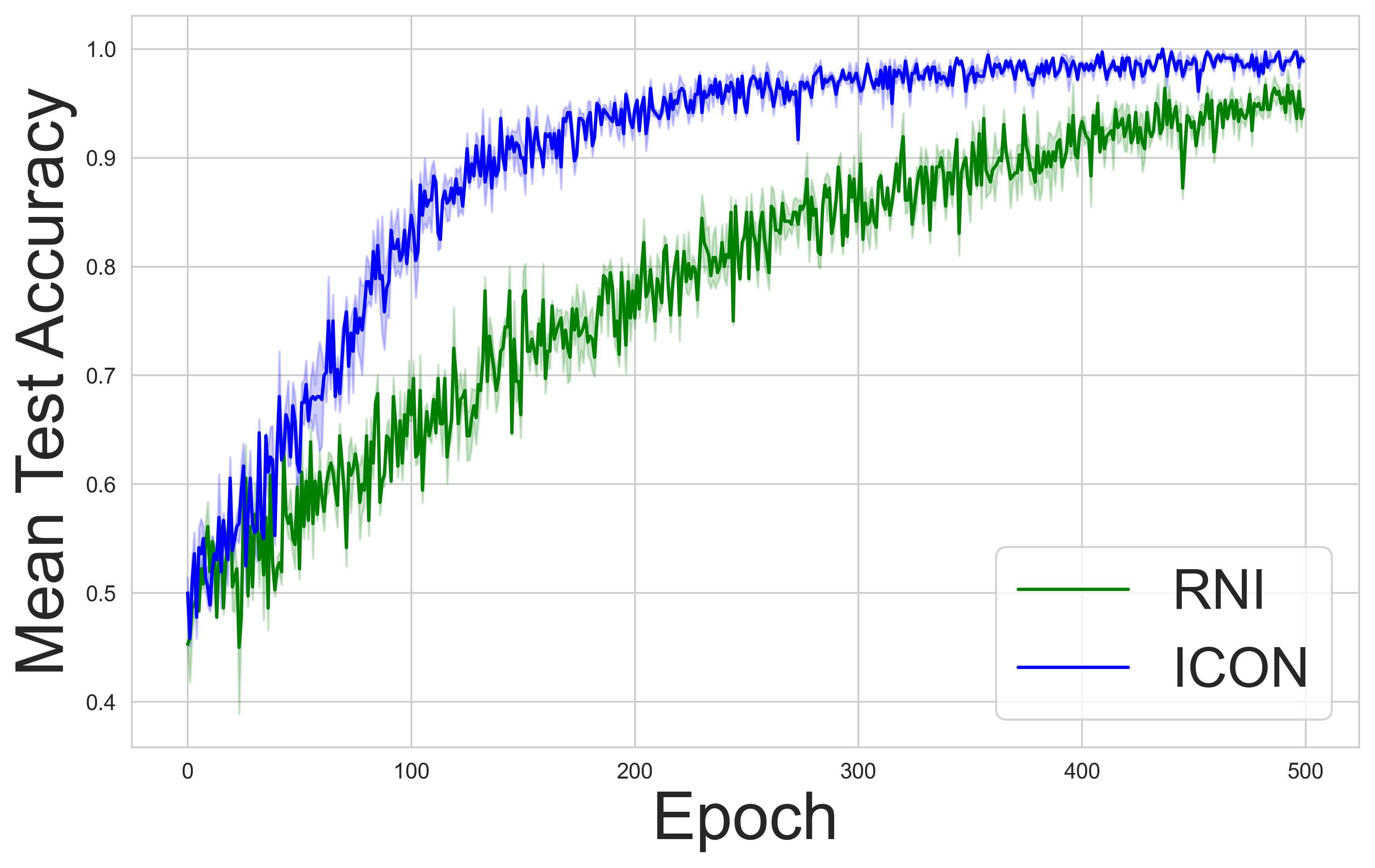
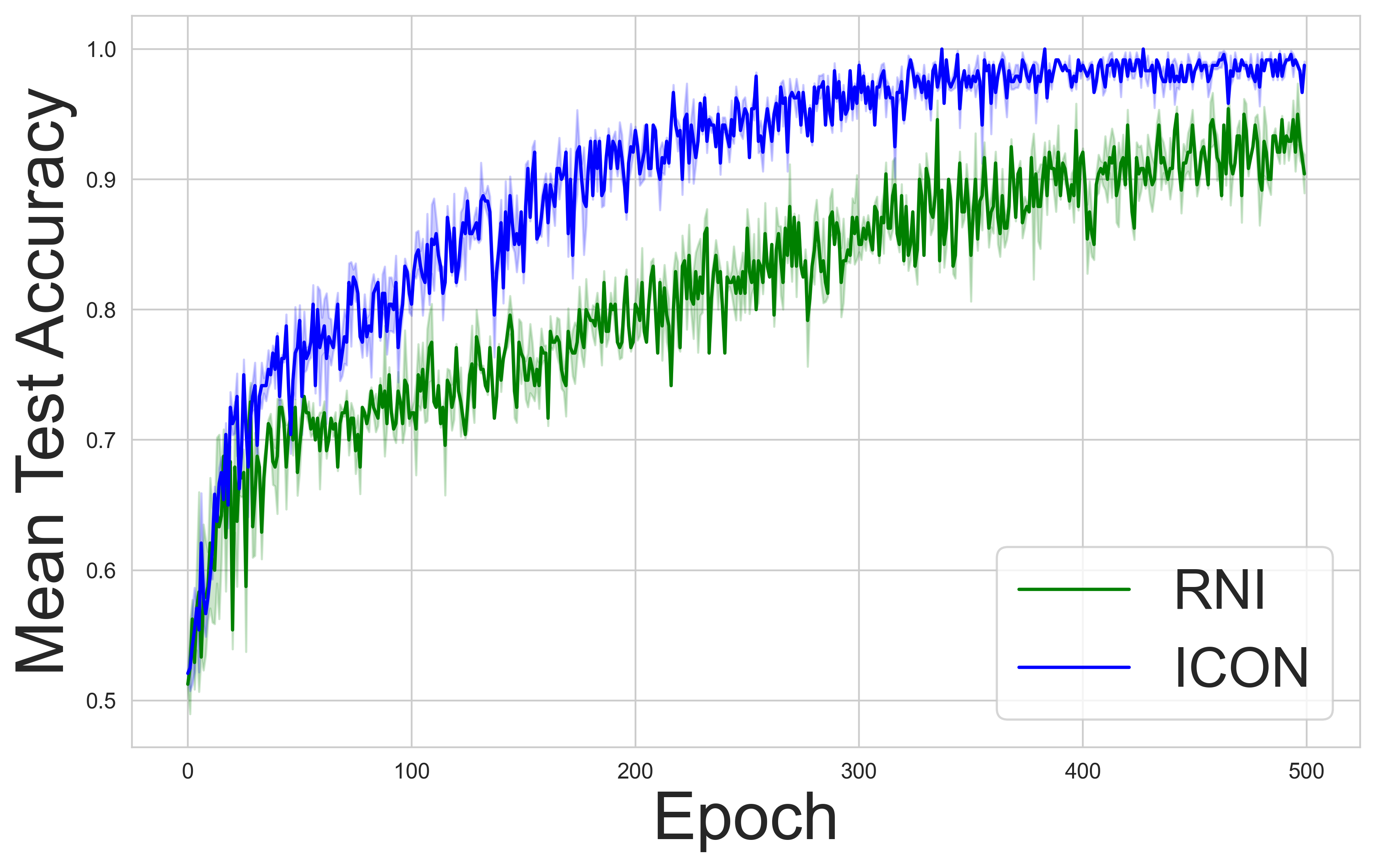
Abboud et al. (2021) presented the EXP and CEXP datasets as an example of the improved expressiveness RNI provides, as these tasks cannot be solved with MPGNNs without IDs. However, it was shown that to improve upon the MPGNNs accuracy, much longer training time is required. In the current experiment, we set out to test if ICON can achieve the same accuracy of RNI while improving the training time.
Datasets
EXP and CEXP (Abboud et al., 2021) contain 600 pairs of graphs (1,200 graphs in total) that cannot be distinguished by 1&2-WL tests. The goal is to classify each graph into one of two isomorphism classes. Splitting is done by stratified five-fold cross-validation. CEXP is a modified version of EXP, where 50% of pairs are slightly modified to be distinguishable by 1-WL. It was shown in (Abboud et al., 2021) that a GraphConv (Abboud et al., 2021) with RNI reaches perfect accuracy on the test set.
Setup
Results
Figure 1 presents the learning curves of accuracy during training for ICON and RNI. Both methods reach a test accuracy of almost 100%, but ICON convergence is faster in both tasks, highlighting the effect of explicit regularization towards IDs-invariance as introduced by ICON vs. an implicit one as done in RNI using random resampling of IDs during training.
7 Future Work
In this section, we discuss several future research directions. An intriguing open question is whether two layers of a GNN with unique identifiers (IDs) suffice to achieve additional expressiveness beyond the 1-WL test.
In Section 4 we demonstrated that three layers already provide greater expressiveness than 1-WL. The question of whether this can be achieved with only two layers would be interesting to study.
We showed that using ID-invariance on all layers does not enhance expressiveness, whereas enforcing invariance solely in the final layer does. Fully understanding the conditions on layers regarding ID-invariance and identifying which functions can be computed under various settings presents an interesting direction for future research.
Our experiments show that ID utilization can be improved with ICON, by learning to produce an invariant network. Another interesting open question is how to design GNNs that benefit from the added theoretical expressiveness of IDs and are invariant to IDs by design. We conjecture that this can be achieved by combining a matching oracle with a GNN architecture.
A matching oracle is a function that takes two nodes from the graph as input and returns 1 if they are the same node and 0 otherwise.
The following result (see appendix for proof) shows that any ID-invariant function can be computed with such an oracle.
Theorem 7.1.
Any ID-invariant function can be computed with a matching oracle.
It would be very interesting to combine such an oracle with Message-Passing GNNs in an effective way, that also results in an improved empirical performance.
8 Conclusions
In this paper, we harness the theoretical power of unique node identifiers (IDs) to enhance the effectiveness of Graph Neural Networks (GNNs). We show that, in practice, the final output of GNNs incorporating node IDs is not invariant to the specific choice of IDs.
We provide a theoretical analysis that motivates an approach which explicitly enforces invariance to IDs in GNNs while taking advantage of their expressive power. Building on our theoretical results, we propose ICON, an explicit regularization technique, which is GNN agnostic.
Through comprehensive experiments, we demonstrate across real-world and synthetic datasets
that ICON considerably improves invariance to node IDs, as well as generalization, extrapolation and training convergence time. These results highlight ICON as an efficient solution for improving the performance of GNNs through IDs utilization, making it a valuable tool for use with any GNN.
References
- Abboud et al. (2021) Abboud, R., İsmail İlkan Ceylan, Grohe, M., and Lukasiewicz, T. The surprising power of graph neural networks with random node initialization, 2021. URL https://arxiv.org/abs/2010.01179.
- Barabasi & Albert (1999) Barabasi, A.-L. and Albert, R. Emergence of scaling in random networks. Science, 286(5439):509–512, 1999. doi: 10.1126/science.286.5439.509. URL http://www.sciencemag.org/cgi/content/abstract/286/5439/509.
- Bechler-Speicher et al. (2024) Bechler-Speicher, M., Amos, I., Gilad-Bachrach, R., and Globerson, A. Graph neural networks use graphs when they shouldn’t, 2024. URL https://arxiv.org/abs/2309.04332.
- Benton et al. (2020) Benton, G., Finzi, M., Izmailov, P., and Wilson, A. G. Learning invariances in neural networks. In Proceedings of NeurIPS, 2020. URL https://arxiv.org/abs/2010.11882.
- Bevilacqua et al. (2022) Bevilacqua, B., Frasca, F., Lim, D., Srinivasan, B., Cai, C., Balamurugan, G., Bronstein, M. M., and Maron, H. Equivariant subgraph aggregation networks, 2022.
- Bouritsas et al. (2023) Bouritsas, G., Frasca, F., Zafeiriou, S., and Bronstein, M. M. Improving graph neural network expressivity via subgraph isomorphism counting. IEEE Transactions on Pattern Analysis and Machine Intelligence, 45(1):657–668, January 2023. ISSN 1939-3539. doi: 10.1109/tpami.2022.3154319. URL http://dx.doi.org/10.1109/TPAMI.2022.3154319.
- Cantürk et al. (2024) Cantürk, S., Liu, R., Lapointe-Gagné, O., Létourneau, V., Wolf, G., Beaini, D., and Rampášek, L. Graph positional and structural encoder. In Salakhutdinov, R., Kolter, Z., Heller, K., Weller, A., Oliver, N., Scarlett, J., and Berkenkamp, F. (eds.), Proceedings of the 41st International Conference on Machine Learning, volume 235 of Proceedings of Machine Learning Research, pp. 5533–5566. PMLR, 21–27 Jul 2024. URL https://proceedings.mlr.press/v235/canturk24a.html.
- Chen et al. (2020) Chen, Z., Chen, L., Villar, S., and Bruna, J. Can graph neural networks count substructures?, 2020. URL https://arxiv.org/abs/2002.04025.
- Dwivedi & Bresson (2021) Dwivedi, V. P. and Bresson, X. A generalization of transformer networks to graphs, 2021. URL https://arxiv.org/abs/2012.09699.
- Eliasof et al. (2023) Eliasof, M., Frasca, F., Bevilacqua, B., Treister, E., Chechik, G., and Maron, H. Graph positional encoding via random feature propagation. In International Conference on Machine Learning, pp. 9202–9223. PMLR, 2023.
- Eliasof et al. (2024) Eliasof, M., Bevilacqua, B., Schönlieb, C.-B., and Maron, H. Granola: Adaptive normalization for graph neural networks. In Proceedings of NeurIPS, 2024.
- Garg et al. (2020a) Garg, V. K., Jegelka, S., and Jaakkola, T. Generalization and representational limits of graph neural networks, 2020a. URL https://arxiv.org/abs/2002.06157.
- Garg et al. (2020b) Garg, V. K., Jegelka, S., and Jaakkola, T. Generalization and representational limits of graph neural networks, 2020b. URL https://arxiv.org/abs/2002.06157.
- Gilmer et al. (2017) Gilmer, J., Schoenholz, S. S., Riley, P. F., Vinyals, O., and Dahl, G. E. Neural message passing for quantum chemistry, 2017.
- Hamilton et al. (2018) Hamilton, W. L., Ying, R., and Leskovec, J. Inductive representation learning on large graphs, 2018.
- Hu et al. (2020) Hu, W., Fey, M., Zitnik, M., Dong, Y., Ren, H., Liu, B., Catasta, M., and Leskovec, J. Open graph benchmark: Datasets for machine learning on graphs, 2020. URL https://arxiv.org/abs/2005.00687.
- Hu et al. (2021) Hu, W., Fey, M., Zitnik, M., Dong, Y., Ren, H., Liu, B., Catasta, M., and Leskovec, J. Open graph benchmark: Datasets for machine learning on graphs, 2021. URL https://arxiv.org/abs/2005.00687.
- Jaderberg et al. (2015) Jaderberg, M., Simonyan, K., Zisserman, A., and Kavukcuoglu, K. Spatial transformer networks. In Advances in neural information processing systems, pp. 2017–2025, 2015.
- Jia et al. (2024) Jia, T., Li, H., Yang, C., Tao, T., and Shi, C. Graph invariant learning with subgraph co-mixup for out-of-distribution generalization. In Proceedings of the AAAI Conference on Artificial Intelligence, volume 38, pp. 8562–8570, 2024.
- Kipf & Welling (2017) Kipf, T. N. and Welling, M. Semi-supervised classification with graph convolutional networks. In International Conference on Learning Representations, 2017. URL https://openreview.net/forum?id=SJU4ayYgl.
- Laptev et al. (2016) Laptev, D., Savinov, N., Buhmann, J. M., and Pollefeys, M. Ti-pooling: transformation-invariant pooling for feature learning in convolutional neural networks. In Proceedings of the IEEE Conference on Computer Vision and Pattern Recognition, pp. 289–297, 2016.
- Loukas (2020) Loukas, A. What graph neural networks cannot learn: depth vs width, 2020. URL https://arxiv.org/abs/1907.03199.
- Morris et al. (2021) Morris, C., Ritzert, M., Fey, M., Hamilton, W. L., Lenssen, J. E., Rattan, G., and Grohe, M. Weisfeiler and leman go neural: Higher-order graph neural networks, 2021.
- Murphy et al. (2019) Murphy, R. L., Rao, V., Rincon, B., and Ribeiro, B. Relational pooling for graph representations. In International Conference on Machine Learning, pp. 4663–4673. PMLR, 2019.
- Papp et al. (2021) Papp, P. A., Martinkus, K., Faber, L., and Wattenhofer, R. Dropgnn: Random dropouts increase the expressiveness of graph neural networks, 2021. URL https://arxiv.org/abs/2111.06283.
- Pellizzoni et al. (2024) Pellizzoni, P., Schulz, T. H., Chen, D., and Borgwardt, K. On the expressivity and sample complexity of node-individualized graph neural networks. In The Thirty-eighth Annual Conference on Neural Information Processing Systems, 2024. URL https://openreview.net/forum?id=8APPypS0yN.
- Sato et al. (2021) Sato, R., Yamada, M., and Kashima, H. Random features strengthen graph neural networks, 2021. URL https://arxiv.org/abs/2002.03155.
- Simard et al. (1998) Simard, P. Y., LeCun, Y. A., Denker, J. S., and Victorri, B. Transformation Invariance in Pattern Recognition — Tangent Distance and Tangent Propagation, pp. 239–274. Springer Berlin Heidelberg, Berlin, Heidelberg, 1998. ISBN 978-3-540-49430-0. doi: 10.1007/3-540-49430-8˙13. URL https://doi.org/10.1007/3-540-49430-8_13.
- Tinhofer (1991) Tinhofer, G. A note on compact graphs. Discrete Applied Mathematics, 30(2):253–264, 1991. ISSN 0166-218X. doi: https://doi.org/10.1016/0166-218X(91)90049-3. URL https://www.sciencedirect.com/science/article/pii/0166218X91900493.
- Veličković et al. (2018) Veličković, P., Cucurull, G., Casanova, A., Romero, A., Liò, P., and Bengio, Y. Graph attention networks. In International Conference on Learning Representations, 2018.
- Wu et al. (2021) Wu, Z., Pan, S., Chen, F., Long, G., Zhang, C., and Philip, S. Y. A comprehensive survey on graph neural networks. IEEE Transactions on Neural Networks and Learning Systems, 32(1):4–24, 2021.
- Xia et al. (2023) Xia, D., Wang, X., Liu, N., and Shi, C. Learning invariant representations of graph neural networks via cluster generalization. In Thirty-seventh Conference on Neural Information Processing Systems, 2023. URL https://openreview.net/forum?id=zrCmeqV3Sz.
- Xu et al. (2019) Xu, K., Hu, W., Leskovec, J., and Jegelka, S. How powerful are graph neural networks? In International Conference on Learning Representations, 2019. URL https://openreview.net/forum?id=ryGs6iA5Km.
- You et al. (2021) You, J., Ying, R., and Leskovec, J. Identity-aware graph neural networks. In Proceedings of the AAAI Conference on Artificial Intelligence, volume 35, pp. 10737–10745, 2021.
Appendix A Proofs
A.1 Proof of Theorem 4.2
We will show that there exists a function that is invariant to IDs with respect to one set of graphs and non-invariant with respect to another set of graphs .
For a given graph , we denote the unique identifier of node as for each node . Let be any graph property that is ID-invariant, such as the existence of the Eulerian path. We consider the following function:
computes the function over the graphs in , and returns the sum of IDs of otherwise. Summing the IDs is not invariant to the IDs’ values. Therefore, is invariant to IDs with respect to graphs in but not with respect to the graphs in .
A.2 Proof of direct implication of Theorem 4.2
In the main text we mention that a direct implication of Theorem 4.2 states that a GNN can be ID-invariant to a train set and non ID-invariant to a test set. This setting only differs from the setting in Theorem 4.2 in that the learned function is now restricted to one that can be realized by a GNN. Indeed, as proven in Abboud et al. (2021), a GNN with IDs is a universal approximator. Specifically, with enough layers and width, an MPGNN can reconstruct the adjacency matrix in some hidden layer, and then compute over it the same function as in the proof of Theorem 4.2.
A.3 Proof of Theorem 4.3
To prove the theorem, we show that a GNN-R that is ID invariant in every layer is equivalent to a GNN without IDs with identical constant values on the nodes. We focus on the case where no node features exist in the data. For the sake of brevity, we assume, without loss of generality, that the IDs of GNN-R are of dimension and that the fixed constant features of the GNN without IDs are of the value . We focus on Message-Passing GNNs. Let GNN-R be a GNN-R with layers that is ID-invariant in every layer. Let GNN’ be a regular GNN with layers that assigns constant features to all nodes. We denote a model up to its ’th layer as . We will prove by induction on the layers that the output of every layer of GNN-R can be realized by the corresponding layers in GNN’. we denote the inputs after the assignments of values to nodes by the networks as for GNN-R and for GNN’.
Base Case - : we need to show that there is such that As is a ID-invariant layer, for any . Specifically, Therefore we can have and then .
Assume that the statement is true up to the layer. We now prove that there is such that .
From the inductive assumption, there is such that . Let us take such . As the ’th layer is ID-invariant, it holds that . Therefore, we can have and then .
A.4 Proof of Theorem 4.4
To prove Theorem 4.4, we will construct a GNN with three layers, where the first two layers are non ID-invariant, and the last layer is ID-invariant, that solves the isInTriangle task. It was already shown that isInTriangle cannot be solved by 1-WL GNNs (Garg et al., 2020a).
Let be a graph with nodes, each assigned with an ID. We assume for brevity that the IDs are of dimension , and assume no other node features are associated with the nodes of .
We use the following notation: in every layer , , each node updates its representation by computing a message using a function , aggregates the messages from its neighbors , , using a function , and updates its representation by combining the outputs of and .
We now construct the GNN as follows.The inputs are .
In the first layer, the message function simply copies the ID of the node, i.e. . The aggregation function, concatenates the messages, i.e. the IDs of the neighbors, in arbitrary order: . Then the update function concatenates its own ID and the list of IDs of its neighbors: . Therefore, in the output of the first layer, the node’s own ID is in position of the representation vector.
The second layer the message function is the identity function, . The aggregation function, again concatenates the messages in arbitrary order: . Then again the update function concatenates the message of the node with the output of the aggregation function: . Therefore, at the output of the second layer, the first entry is the node’s own ID, followed the the ID’s of its direct neighbors, followed the lists of IDs of the neighbors of its neighbors.
Notice that the first and second layers are not ID-invariant, as replacing the ID values will result in a different vector.
In the final layer, the message and aggregate functions are the same as in the second layer, i.e., and . The update function performs a matching between the ID of the node, which appears in the first entry of the message, , and the output of the aggregation function entries. This matching examines if the ID of the node appears in the messages from three-hop neighbors. If it does, this means the node is part of a triangle, as it sees its own ID again in 3 hops. Then outputs 1; otherwise, it outputs 0. This third layer is ID-invariant, as its outputs depend on the re-appearance of the same IDs, without dependency on their values.
A.5 Proof of Theorem 7.1
Let be an equivariant function of graphs that is also ID-invariant. We will demonstrate that can be expressed using a matching oracle. Let be a matching oracle defined as follows:
Assume we have a serial program that computes . We will compute using a serial function that utilizes the oracle . The function incorporates caching Let Cache denote a cache that stores nodes with an associated value to each node.
The function operates as , except for the follows:
-
(a)
When needs to access the ID of a node , checks whether already exists in the cache by matching with each node stored in the cache using the oracle .
-
(b)
If is found in the cache, retrieves and returns the value associated with it.
-
(c)
If is not found in the cache, adds it to the cache and assigns a new value to as , and return its value.
By the assumption that is invariant under IDs, we have .
Appendix B Additional Experimental Details
OGB datasets
The datasets’ statistics are presented in Table 6.
| Dataset | # Graphs | Avg # Nodes | Avg # Edges | # Node Features | # Classes |
|---|---|---|---|---|---|
| ogbn-arxiv | 1 | 169,343 | 1,166,243 | 128 | 40 |
| ogbg-molhiv | 41,127 | 25.5 | 27.5 | 9 | 2 |
| ogbg-molbace | 1,513 | 34.1 | 36.9 | 9 | 2 |
| ogbg-molbbbp | 2,039 | 24.1 | 26.0 | 9 | 2 |
isInTriangle
The isInTriangle task is a binary node classification where the goal is to determine whether a given node is part of a triangle. The dataset consists of 100 graphs with 100 nodes each, generated using the preferential attachment (BA) model (Barabasi & Albert, 1999), in which graphs are constructed by incrementally adding new nodes with edges and connecting them to existing nodes with a probability proportional to the degrees of those nodes. We adopt an inductive setting, where the graphs used during testing are not included in the training set. We used for all the training graphs.
EXP and CEXP
We followed the protocol of Abboud et al. (2021) and used Adam optimizer with a learning rate of . The network has GraphConv layers followed by a sum-pooling and a layer readout function. All hidden layers have dimensions, and we used random features and we did not discard the original features in the data.
Hyper-Parameters
For all experiments, we use a fixed drouput rate of 0.1 and Relu activations. We tuned the learning rate in , batch size in , number of layers in , and hidden dimensions in .