Improving Collision-Free Success Rate For Object Goal Visual Navigation Via Two-Stage Training With Collision Prediction

Abstract

The object goal visual navigation is the task of navigating to a specific target object using egocentric visual observations. Recent end-to-end navigation models based on deep reinforcement learning have achieved remarkable performance in finding and reaching target objects. However, the collision problem of these models during navigation remains unresolved, since the collision is typically neglected when evaluating the success. Although incorporating a negative reward for collision during training appears straightforward, it results in a more conservative policy, thereby limiting the agent’s ability to reach targets. In addition, many of these models utilize only RGB observations, further increasing the difficulty of collision avoidance without depth information. To address these limitations, a new concept—collision-free success is introduced to evaluate the ability of navigation models to find a collision-free path towards the target object. A two-stage training method with collision prediction is proposed to improve the collision-free success rate of the existing navigation models using RGB observations. In the first training stage, the collision prediction module supervises the agent’s collision states during exploration to learn to predict the possible collision. In the second stage, leveraging the trained collision prediction, the agent learns to navigate to the target without collision. The experimental results in the AI2-THOR environment demonstrate that the proposed method greatly improves the collision-free success rate of different navigation models and outperforms other comparable collision-avoidance methods.

I Introduction

Object goal visual navigation poses a major challenge to robots, which requires them to navigate to a specific object instance based on visual observations. Recent studies have achieved promising results in solving this task using deep reinforcement learning (DRL) to train an end-to-end navigation policy, many of which use only RGB observations[1, 2, 3, 4, 5, 6, 7, 8, 9]. While some studies implicitly learn the visual representation[1, 2, 3], others leverage the object or region relationships by introducing knowledge graphs[4, 5, 6] or context information[7, 8, 9] to learn a more robust navigation policy.

Although these models have made impressive progress in the navigation performance of reaching the target, collision avoidance of the navigation has not been thoroughly investigated. Typically, when evaluating these models, a navigation episode is still considered a success even if collisions occur during the navigation trajectories to the target object. In addition, the reward function of many models[1, 2, 3, 4, 5, 6, 7, 8, 9] is not designed to penalize collision during training, since the negative reward leads to a more conservative navigation policy and thus a lower success rate. However, this oversight is particularly problematic when considering real-world robotic applications, especially for the models relying solely on RGB observations, which complicates collision avoidance in the absence of depth information.

To help the agent using only RGB observations find a collision-free path towards the target, this letter proposes a two-stage reinforcement learning training method with a collision prediction module. In the first stage, the collision prediction module learns to predict the collision probability from visual observations by supervising the agent’s trajectories. In the second stage, the reward function is reshaped with a collision penalty. The agent is then trained to navigate to the target without colliding with obstacles with the help of the learned collision prediction module. Evaluated with the new metric collision-free success, extensive experiments in the AI2Thor environment show great improvements in the collision-free success rate of selected navigation models using the proposed method compared to other collision avoidance methods.

II Related Work

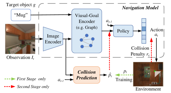
Figure 1: The illustration of the two-stage training method with collision prediction. In the first stage, the collision prediction module is trained by supervising the collision state of the navigation agent. In the second stage, the learned collision prediction is inputted into the agent to help it learn navigation under collision penalty.

II-A Object-Goal Visual Navigation

Object-goal visual navigation refers to navigating to the target object using visual observations. To solve this task, a number of studies have been proposed to successfully find the target, including but not limited to map-based approaches and end-to-end models. Map-based approaches incrementally construct semantic maps[10, 11] or topological maps[12] of the environment during exploration, which requires precise positioning and depth images. End-to-end models directly map image embeddings and goal embeddings to actions using deep reinforcement learning. Many studies utilized only RGB images to train the agent and achieved remarkable navigation performance with various network designs, including the meta learning[1], visual transformer[2, 3], knowledge graph[4, 5, 6], context information[7, 8, 13, 14], layout information[15], attention mechanisms[16, 9], subtask learning[17], etc. For example, Du et al.[2] utilized a visual transformer[18] to learn informative visual representations during navigation. Xu et al.[6] introduced the CLIP model[19] to align the knowledge graph with visual perception, achieving remarkable navigation performance.

These models improve the success rate in navigating to the target using only RGB images without explicitly considering the collision in the trajectory. Their navigation performance is possibly degraded if the collision is taken into account when calculating the success rate. In this letter, a two-stage training method of reinforcement learning with collision prediction is proposed to improve the collision-free success rate of the existing navigation models.

II-B Collision Avoidance of DRL Visual Navigation

Collision avoidance during navigation is an indispensable ability for robots. A typical way of reducing collisions of the DRL visual navigation is to reshape the reward function with a collision penalty[20, 21, 22]. Xiao et al.[22] introduced a single-step reward and collision penalty to avoid collisions. However, the negative reward from collisions tends to train a more conservative navigation policy, hindering the improvement of the success rate. Wu et al.[23] predicted the collision in advance as an auxiliary task of imitation learning to improve safety during navigation, which requires expert trajectories to train the navigation policy.

In this letter, we propose a two-stage training method with collision prediction to improve the collision-free success rate of object-goal visual navigation without expert trajectories. In the first stage, the agent is free to explore environments without the collision penalty, while the collision prediction module supervises collisions that occur during the agent’s exploration. In the second stage, the agent learns to navigate to the target while avoiding collisions with the collision penalty and the help of the learned collision prediction. The experimental results show the advantage of our method compared to other collision avoidance methods.

III Task Definition

In this letter, the agent is required to navigate to a set of predefined target objects $G$ using only egocentric RGB images. The initial position of the agent is randomly initialized in each navigation episode. At each timestep $t$, the agent predicts its action $a_{t}\in\mathcal{A}$ based on the current RGB image $I_{t}$ and the target object $g\in G$ by employing a policy network $\pi\left(a_{t}\mid I_{t},g;\theta\right)$. Here, $\theta$ is the weight of the policy network. The action space $\mathcal{A}$ is discretized as {MoveAhead, RotateLeft, RotateRight, LookUp, LookDown, Done}. The step size of MoveAhead is 0.25m. The agent’s rotation angle and the camera’s vertical tilting angle are $45^{\circ}$ and $30^{\circ}$, respectively. The Done action terminates the current navigation episode.

In previous work, an episode is determined to be successful if the agent chooses the Done action and the target object is visible, which means the target object appears in the agent’s current RGB image and within a distance of 1.5m from it. We introduce collision-free success in this letter, i.e., an episode is considered as a success not only if the above conditions are met but also if no collision occurs during the navigation. This letter proposes a training method aiming to improve the collision-free success rate of the existing navigation models.

IV Two-Stage Training With Collision Prediction

IV-A Two-Stage Training of Navigation Model

The proposed two-stage training method is illustrated in Fig. 1. The existing navigation model usually contains an image encoder to process the RGB observation and a visual-goal encoder to encode features of the observation and the target object $g$. All the features processed by encoders are then concatenated to predict the possible action by passing through a policy network $\pi$, which usually contains several long-short term (LSTM) layers and fully connected networks (FCN). In the proposed training method, an additional collision prediction module is added to the existing navigation model. At each time step $t$, the module predicts collision probability $\hat{p}_{t}$ of the agent moving forward from the current RGB observation $I_{t}$, i.e., $\hat{p}_{t}=P(I_{t};\phi)$, where $\phi$ is the weight of the collision prediction module. The agent then predicts its action based on the current RGB observation $I_{t}$ and target object $g$ as well as the predicted collision probability $\hat{p}_{t}$, i.e., $\pi(a_{t}\mid I_{t},g,\hat{p}_{t};\theta)$, where $\theta$ is the weight of the policy network $\pi$.

In the first training stage, the agent is encouraged to fully explore the environments to find the target without explicitly considering collisions. The reward function includes no collision penalty and is the same as the original reward $r_{\rm o}$ that varies from the selected navigation models. The collision prediction module concurrently learns to predict collision probability when the agent takes the MoveAhead action by supervising collisions along the agent’s trajectories. The input of collision probability into the policy network is set to zero in this training stage to avoid inaccurate collision prediction affecting navigation. After the training of the first stage, the agent learns a bolder policy that has a higher success rate in finding the target but does not take collisions into account.

In the second training stage, the agent learns to navigate to the target while avoiding collisions with the help of the trained collision prediction. A collision reward $r_{c}$ is added to the reward function, which penalizes the agent when collisions occur. The predicted collision probability learned from the first stage is inputted into the navigation policy to help it identify the possible collision of moving forward, avoiding over-conservative policy caused by the collision penalty. The weight of the collision prediction stops updating in this stage for not overfitting the training set.

IV-B Collision Prediction

Since only the MoveAhead action in the action space possibly causes collisions, the collision prediction is treated as a binary classification problem. The designed collision prediction module contains two LSTM layers with a hidden state size of 512. It takes the current RGB observation $I_{t}$ and the last action $a_{t-1}$ as the input and outputs the probability of collision $\hat{p}_{t}$ of the agent moving forward. The collision prediction module is trained by supervising the navigation trajectories in the first training stage. At each time step where the agent takes the MoveAhead action, the module receives a binary collision state $p_{t}$ with 1 denoting collision from the environment and updates its weight by minimizing the collision prediction loss $L_{\rm c}$ as

$$L_{\rm c}=-p_{t}\log\hat{p}_{t}-(1-p_{t})\log(1-\log\hat{p}_{t})$$ (1)

IV-C Reward Function

The reward function at each time step $t$ is designed as

$$r=\left\{\begin{array}[]{ccl}r_{\rm o}&&E<E_{1}\\ r_{\rm o}+r_{\rm c}&&E_{1}\leq E<E_{1}+E_{2}\end{array}\right.$$ (2)

Here, $r_{\rm o}$ and $r_{\rm c}$ are the original reward and collision reward, respectively. $E$ is the current number of episodes. $E_{1}$ and $E_{2}$ are the total number of episodes in the first and second training stages, respectively. $r_{\rm c}$ is set to -0.5 when the agent collides with obstacles, and 0 otherwise. The setting of $r_{\rm o}$ is based on the selected navigation models. A typical reward setting is when the agent takes the Done action and the target object is visible, it receives a large positive reward, and a small time penalty otherwise. In [7] and [9], a partial reward is additionally introduced to better learn object relationships.

1

2repeat

3    Randomize the scene, agent’s position and goal $g$;

4    Reset time step $t\leftarrow 0$;

5    repeat

6       Reset gradients $d\theta\leftarrow 0$, $d\theta_{v}\leftarrow 0$, $d\phi\leftarrow 0$;

7       Synchronize $\theta^{\prime}\leftarrow\theta$, $\theta_{v}^{\prime}\leftarrow\theta_{v}$, $\phi^{\prime}\leftarrow\phi$;

8       $t_{\rm start}\leftarrow t$;

9       repeat

10          Get image $I_{t}$;

11          Predict collision $\hat{p}_{t}\leftarrow P(I_{t};\phi^{\prime})$;

12          if $E<E_{1}$ then

13            Receive observation $O_{t}\leftarrow(I_{t},g,0)$;

14             Perform $a_{t}$ through $\pi(a_{t}\mid O_{t};\theta^{\prime})$;

15             Receive collision state $p_{t}$ and reward $r_{t}\leftarrow r_{{\rm o},t}$;

16         else

17            Receive observation $O_{t}\leftarrow(I_{t},g,\hat{p}_{t})$;

18             Perform $a_{t}$ through $\pi(a_{t}\mid O_{t};\theta^{\prime})$;

19             Receive collision state $p_{t}$ and reward $r_{t}\leftarrow r_{{\rm o},t}+r_{{\rm c},t}$;

20          end if

21         $t\leftarrow t+1$;

22         

23      until $a_{t}=$ Done or $t-t_{\rm start}=t_{\rm max}$;

24      $R\leftarrow 0$ if $a_{t}=$ Done else $V(O_{t};\theta_{v}^{\prime})$;

25       for $i\in\{t-1,...,t_{\rm start}\}$ do

26          $R\leftarrow r_{i}+\gamma R$;

27          $\delta_{t}\leftarrow R-V(O_{i};\theta_{v}^{\prime})$;

28          $d\theta\leftarrow d\theta+\nabla_{\theta^{\prime}}\log\pi(a_{i}\mid O_{i};\theta^{\prime})\delta_{t}$;

29          $d\theta_{v}\leftarrow d\theta_{v}+\nabla_{\theta_{v}^{\prime}}\delta_{t}^{2}$;

30          if $E<E_{1}$ and $a_{i}=$ MoveAhead then

31             $d\phi\leftarrow d\phi+\nabla_{\phi^{\prime}}L_{{\rm c},i}$ using Eq. (1);

32          end if

33         

34       end for

35      Perform asynchronous update of $\theta$, $\theta_{v}$ and $\phi$;

36      

37   until $a_{t}=$ Done;

38   $E\leftarrow E+1$;

39until $E=E_{1}$+$E_{2}$;

Algorithm 1 Pseudocode for each A3C thread using two-stage training method with collision prediction.

Following previous works [6, 5, 9, 4, 7, 15], A3C [24] reinforcement learning method is adopted to train the navigation agent. Assume the following variable definitions: shared global parameters of the actor network $\theta$, the critic network $\theta_{v}$, and collision prediction module $\phi$, their thread-specific parameters $\theta^{\prime}$, $\theta_{v}^{\prime}$ and $\phi^{\prime}$, and the global shared episode counter $E$. The actor network learns a policy $\pi(a_{t}\mid O_{t};\theta)$, which predicts the action $a_{t}$ based on the observation $O_{t}$. The critic network estimates the state-value function $V(O_{t};\theta_{v})$ based on the observation $O_{t}$. The collision prediction module predicts collision probability $P(I_{t};\phi)$ using the current RGB image $I_{t}$. The pseudocode for each A3C thread using the proposed training method is summarized in Algorithm 1.

V Experiments

V-A Experimental Setup

We deploy the proposed training method on the selected navigation models and compare it to other collision avoidance methods in the AI2-THOR embodied AI environment[25]. The environment consists of 120 near photo-realistic indoor room scenes with four room types, i.e., kitchen, living room, bedroom and bathroom. Each navigation model is trained for a total of 3 million episodes using 32 asynchronous agents with 1 million episodes in the first training stage ($E_{1}=1,000,000$) and 2 million episodes in the second training stage ($E_{2}=2,000,000$). The weight of model is updated by Adam optimizer with a learning rate of 0.0001.

The metrics including the collision-free success rate (CF-SR) and the collision-free success weighted by path length (CF-SPL)[26] are used for evaluation. The collision-free success indicates that no collision is allowed during a success navigation. CF-SR is calculated as ${\frac{1}{N}\sum^{N}_{i=1}S_{i}}$ where $N$ is the number of episodes and $S_{i}$ is the collision-free success indicator of the $i$-th episode with 1 representing success and 0 otherwise. CF-SPL is calculated as ${\frac{1}{N}\sum^{N}_{i=1}S_{i}\frac{d_{i}^{*}}{\max(d_{i}^{*},d_{i})}}$ where $d_{i}$ and $d_{i}^{*}$ represent the agent’s path length and the optimal path length from its initial position to the target object in the $i$-th episode, respectively. Five independent trials are run for each navigation model and the results are presented as mean$\pm$standard deviation. We use an upward arrow $\uparrow$ to indicate the increase in the SR/SPL after deploying the proposed training method.

V-B Deployment on Navigation Models

We deploy the proposed training method on the following navigation models. Baseline[27] concatenates the image feature with the word embedding or class label of the target object as the input of the navigation policy network. HOZ[5] utilizes hierarchical object-to-zone graph to guide the agent. L-sTDE[15] calculates the object layout gap between different scenes to adjust the prediction of the navigation policy. AKGVP[6] leverages the language-image pertaining model to align knowledge graph with visual perception, achieving state-of-the-art navigation performance. MJOLNIR-r[7] utilizes context vectors and the graph convolutional neural network to learn parent-target hierarchical object relationships. TDANet[9] learns spatial and semantic relationships of objects through a novel target attention module and the Siamese network design. Since TDANet only uses object detection results, we add image features encoded by the CLIP[19] model to TDANet for collision prediction of the proposed method.

According to the training data of the selected navigation models, We use two offline datasets from the AI2THOR environment, which vary in target objects, labels of object detection, etc. The setting of Offline Data 1 follows [6] with 80 rooms as the training set and 20 rooms as the test set. The setting of Offline Data 2 follows [7] with 80 rooms as the training set and 40 rooms as the test set.

The evaluation results of different models using the proposed training method are reported in Table I. It is observed that the proposed method improves navigation performance satisfactorily with higher collision-free SR and SPL for all the selected models. In Offline Data 1, L-sTDE and AKGVP using the proposed method increase CF-SR by 5.3% and 3.9%, and CF-SPL by 1.9% and 1.2%, respectively. In Offline Data 2, MJOLNIR-r and TDANet increase CF-SR by 8.5% and 7.0%, and CF-SPL by 3.1% and 2.4%, respectively, after using the proposed method.

Figure 2 visualizes the sampled paths of L-sTDE model before and after using the proposed training method. After using the proposed method, L-sTDE bypasses obstacles and maintains a distance from them. For example, in Fig. 2(b), the agent of the original L-sTDE gets stuck in front of the desk, while the agent using the proposed method rounds the corner of the table and gets closer to the target.

TABLE I: The collision-free SR and SPL of different models in the test set before&after using the proposed method in AI2-THOR.

Data	Model	CF-SR(%)		CF-SPL(%)
Offline Data 1[6]	Baseline[27]	55.8$\pm$2.7		32.2$\pm$1.8
	HOZ[5]	58.1$\pm$0.9		33.2$\pm$0.5
	L-sTDE[15]	60.0$\pm$0.4		34.0$\pm$1.1
	AKGVP[6]	70.5$\pm$0.7		40.4$\pm$0.8
	ours(Baseline)	59.3$\pm$1.0	3.5$\uparrow$	33.1$\pm$1.5	0.9$\uparrow$
	ours(HOZ)	60.2$\pm$1.3	2.1$\uparrow$	34.1$\pm$0.7	0.9$\uparrow$
	ours(L-sTDE)	65.3$\pm$0.6	5.3$\uparrow$	35.9$\pm$0.9	1.9$\uparrow$
	ours(AKGVP)	74.4$\pm$0.7	3.9$\uparrow$	41.6$\pm$0.5	1.2$\uparrow$
Offline Data 2[7]	Baseline[27]	27.1$\pm$1.1		8.4$\pm$0.4
	MJOLNIR-r[7]	47.2$\pm$4.1		17.9$\pm$2.1
	TDANet[9]	53.5$\pm$1.5		23.4$\pm$1.2
	ours(Baseline)	30.1$\pm$0.7	3.0$\uparrow$	9.5$\pm$0.1	1.1$\uparrow$
	ours(MJOLNIR-r)	55.8$\pm$5.0	8.5$\uparrow$	21.0$\pm$2.3	3.1$\uparrow$
	ours(TDANet)	60.5$\pm$2.3	7.0$\uparrow$	25.8$\pm$0.7	2.4$\uparrow$

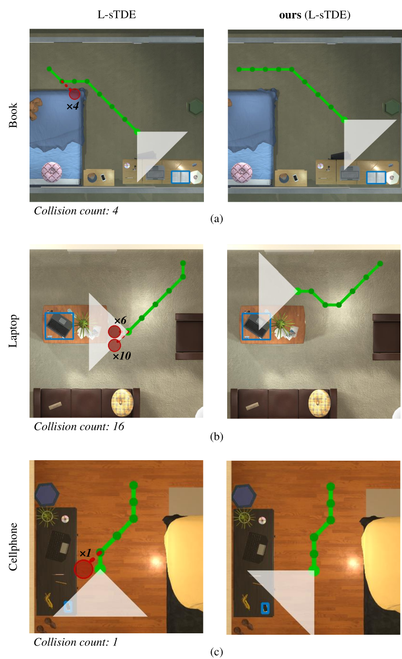
Figure 2: Three sampled navigation paths of L-sTDE[15] model before & after using the proposed training method. The failure actions that cause collisions are marked using red circles with $\times N$ denoting the number of failure actions in the same place. Target objects are marked with blue bounding boxes.

V-C Comparison With Other Collision Avoidance Methods

To demonstrate the advantage of the proposed method, we use L-sTDE trained in Offline Data 1 as the baseline model to compare different collision avoidance methods. The following collision avoidance method is used to compare. Reward only adds a negative reward $r_{\rm c}=-0.1$ to the reward function when the collision occurs. Xiao et al.[22] combines the collision reward $r_{\rm c}=-0.1$ with a single-step reward, i.e., $r_{s}=\lambda(d_{t-1}-d_{t})$. Here, $d_{t-1}$ and $d_{t}$ denote the path length from the agent to the target at time steps $t-1$ and $t$, respectively. $\lambda$ is a scaling factor and is set to 0.01 in this letter. Wu et al.[23] jointly optimizes the navigation policy with a collision prediction network by sharing the same image feature encoder.

The navigation performance using different methods in the test set of AI2-THOR is shown in Table II. The proposed method achieves the greatest navigation performance with CF-SR of 65.3% (5.3%$\uparrow$) and CF-SPL of 35.9% (1.9%$\uparrow$), while other methods show limited improvement in CF-SR ($<2\%$$\uparrow$) and CF-SPL($<1\%$$\uparrow$). Figure 3 shows the learning curves of CF-SR using different collision avoidance methods during training. In the first training stage ($E_{1}$) of the proposed method, the agent learns to find the target and predict collision together without collision penalty. Its CF-SR increases similarly to the method proposed by Wu et al. In the second stage, the agent then learns to navigate to the target while avoiding collision using the learned collision prediction. As shown in Fig. 3, the CF-SR using the proposed method increases rapidly and reaches the highest value of around 80% in the second training stage ($E_{2}$). We also observe that the methods Reward and Xiao et al. that only change the reward function and add a penalty for collision learn a more conservative navigation policy with limited improvements of CF-SR both in the training and test sets. The results demonstrate that the proposed method achieves the largest increase in the collision-free navigation success rate compared to other methods.

TABLE II: The collision-free SR and SPL of L-sTDE[15] using different collision avoidance methods in AI2-THOR.

Method	CF-SR(%)		CF-SPL(%)
L-sTDE[15]	60.0$\pm$0.4		34.0$\pm$1.1
Reward	61.2$\pm$2.3	1.2$\uparrow$	34.2$\pm$1.2	0.2$\uparrow$
Xiao et al.[22]	61.5$\pm$1.7	1.5$\uparrow$	34.2$\pm$1.4	0.2$\uparrow$
Wu et al.[23]	61.6$\pm$1.7	1.6$\uparrow$	34.4$\pm$0.5	0.4$\uparrow$
ours	65.3$\pm$0.6	5.3$\uparrow$	35.9$\pm$0.9	1.9$\uparrow$

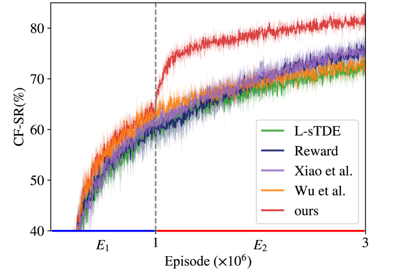
Figure 3: The learning curves of CF-SR using different collision avoidance methods in the training set.

V-D Ablation Study

Following the experimental setting in Section V-C, ablation studies are conducted using the two-stage training only (Stage Only) and the collision prediction only (CP Only) methods. The Stage Only method removes the collision prediction module and retains collision reward $r_{c}=-0.5$ in the second training stage. The CP Only method updates the collision prediction module and inputs the collision probability into the navigation policy throughout the training process without the collision reward.

The CF-SR and CF-SPL of ablation studies in the test and training sets are shown in Table III and Fig. 4, respectively. The two-stage training contributes the most to the performance of the proposed method, which increases the CF-SR and CF-SPL in the test set by 3.3% and 1.3%, respectively. With the two-stage training method, the agent first learns to find the target and then to avoid collisions during navigation, avoiding the more conservative navigation policy learned by directly adding a collision penalty.

Although the CP Only method reaches the highest CF-SR in the training set, it shows the lowest improvements in the test set. The possible reason is that the update of the collision prediction module throughout the training phase causes overfitting, since there is decreased collision and change in the navigation trajectories in the later training phase with less exploration. As shown in Fig. 4, the CF-SR of the CP Only model reaches above 80%. In addition, the navigation policy using the CP Only method without the collision reward from the environment relies heavily on the collision prediction results, which are nearly perfect in the training set but worse in the test set. In comparison, The proposed method only trains the collision prediction in the first stage and inputs it into the navigation policy in the second stage with the collision reward, which avoids overfitting and further improves the navigation performance. The ablation studies show the effectiveness of the proposed training method.

TABLE III: Results of ablation study based on L-sTDE[15] model in the test set in AI2-THOR.

Method	CF-SR(%)		CF-SPL(%)
L-sTDE[15]	60.0$\pm$0.4		34.0$\pm$1.1
Stage Only	63.3$\pm$0.5	3.3$\uparrow$	35.3$\pm$0.2	1.3$\uparrow$
CP Only	60.2$\pm$1.3	0.3$\uparrow$	33.5$\pm$1.3	0.5$\downarrow$
ours	65.3$\pm$0.6	5.3$\uparrow$	35.9$\pm$0.9	1.9$\uparrow$

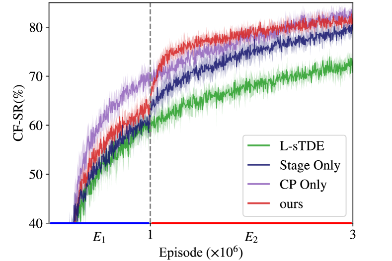
Figure 4: The CF-SR learning curves of ablation studies in the training set.

VI Conclusion

This letter proposed a two-stage training method with collision prediction to improve the collision-free success rate of the existing navigation models. The collision prediction module was trained in the first training stage by supervising the agent’s collision state during exploration. In the second training stage, the agent was trained to find a collision-free path to the target object with the help of collision prediction. The proposed training method was deployed in different navigation models and compared to other collision avoidance methods in the AI2-THOR environment. The experiment results demonstrated the navigation models using the proposed training method successfully improved the navigation performance considering collisions, achieving higher collision-free success rate than using other collision avoidance methods. The ablation studies further showed the effective design of the proposed training method.

In future work, we plan to deploy the navigation model trained using the proposed method in real household environments and investigate the sim-to-real problems to further improve navigation performance.

References

- [1] M. Wortsman, K. Ehsani, M. Rastegari, A. Farhadi, and R. Mottaghi, “Learning to learn how to learn: Self-adaptive visual navigation using meta-learning,” in Proc. IEEE/CVF Conf. Comput. Vis. Pattern Recognit., 2019, pp. 6743–6752.
- [2] H. Du, X. Yu, and L. Zheng, “VTNet: Visual transformer network for object goal navigation,” in Proc. Int. Conf. Learn. Representations, 2021, pp. 1–16.
- [3] R. Fukushima, K. Ota, A. Kanezaki, Y. Sasaki, and Y. Yoshiyasu, “Object memory transformer for object goal navigation,” in Proc. Int. Conf. Robot. Automat., 2022, pp. 11 288–11 294.
- [4] H. Du, X. Yu, and L. Zheng, “Learning object relation graph and tentative policy for visual navigation,” in Proc. Eur. Conf. Comput. Vision, 2020, pp. 19–34.
- [5] S. Zhang, X. Song, Y. Bai, W. Li, Y. Chu, and S. Jiang, “Hierarchical object-to-zone graph for object navigation,” in Proc. IEEE/CVF Int. Conf. Comput. Vis., 2021, pp. 15 110–15 120.
- [6] N. Xu, W. Wang, R. Yang, M. Qin, Z. Lin, W. Song, C. Zhang, J. Gu, and C. Li, “Aligning knowledge graph with visual perception for object-goal navigation,” in IEEE Int. Conf. Robot. Automat., 2024, pp. 5214–5220.
- [7] A. Pal, Y. Qiu, and H. Christensen, “Learning hierarchical relationships for object-goal navigation,” in Proc. Conf. Robot Learn., vol. 155, 2021, pp. 517–528.
- [8] R. Druon, Y. Yoshiyasu, A. Kanezaki, and A. Watt, “Visual object search by learning spatial context,” IEEE Robot. Automat. Lett., vol. 5, no. 2, pp. 1279–1286, 2020.
- [9] S. Lian and F. Zhang, “Tdanet: Target-directed attention network for object-goal visual navigation with zero-shot ability,” IEEE Robot. Automat. Lett., vol. 9, no. 9, pp. 8075–8082, 2024.
- [10] S. Y. Gadre, M. Wortsman, G. Ilharco, L. Schmidt, and S. Song, “Cows on pasture: Baselines and benchmarks for language-driven zero-shot object navigation,” in Proc. IEEE/CVF Conf. Comput. Vis. Pattern Recognit., 2023, pp. 23 171–23 181.
- [11] M. Chang, T. Gervet, M. Khanna, S. Yenamandra, D. Shah, S. Y. Min, K. Shah, C. Paxton, S. Gupta, D. Batra, R. Mottaghi, J. Malik, and D. S. Chaplot, “Goat: Go to any thing,” 2023, arXiv:2311.06430.
- [12] P. Wu, Y. Mu, B. Wu, Y. Hou, J. Ma, S. Zhang, and C. Liu, “Voronav: Voronoi-based zero-shot object navigation with large language model,” in Proc. Int. Conf. Mach. Learn., 2024. [Online]. Available: https://openreview.net/forum?id=Va7mhTVy5s
- [13] Q. Zhao, L. Zhang, B. He, H. Qiao, and Z. Liu, “Zero-shot object goal visual navigation,” in Proc. IEEE Int. Conf. Robot. Automat., 2023, pp. 2025–2031.
- [14] F.-F. Li, C. Guo, H. Zhang, and B. Luo, “Context vector-based visual mapless navigation in indoor using hierarchical semantic information and meta-learning,” Complex Intell. Syst., vol. 9, pp. 2031–2041, 2022.
- [15] S. Zhang, X. Song, W. Li, Y. Bai, X. Yu, and S. Jiang, “Layout-based causal inference for object navigation,” in Proc. IEEE/CVF Conf. Comput. Vis. Pattern Recognit., 2023, pp. 10 792–10 802.
- [16] B. Mayo, T. Hazan, and A. Tal, “Visual navigation with spatial attention,” in Proc. IEEE/CVF Conf. Comput. Vis. Pattern Recognit., 2021, pp. 16 893–16 902.
- [17] A. Devo, G. Mezzetti, G. Costante, M. L. Fravolini, and P. Valigi, “Towards generalization in target-driven visual navigation by using deep reinforcement learning,” IEEE Trans. Robot., vol. 36, no. 5, pp. 1546–1561, 2020.
- [18] A. Vaswani, N. Shazeer, N. Parmar, J. Uszkoreit, L. Jones, A. N. Gomez, L. Kaiser, and I. Polosukhin, “Attention is all you need,” in Proc. Advances Neural Inf. Process. Syst., 2017, pp. 6000–6010.
- [19] A. Radford, J. W. Kim, C. Hallacy, A. Ramesh, G. Goh, S. Agarwal, G. Sastry, A. Askell, P. Mishkin, J. Clark, G. Krueger, and I. Sutskever, “Learning transferable visual models from natural language supervision,” in Proc. Int. Conf. Mach. Learn., vol. 139, 2021, pp. 8748–8763.
- [20] K. Lobos-Tsunekawa, F. Leiva, and J. Ruiz-del Solar, “Visual navigation for biped humanoid robots using deep reinforcement learning,” IEEE Robot. Automat. Lett., vol. 3, no. 4, pp. 3247–3254, 2018.
- [21] Y. Chen, G. Chen, L. Pan, J. Ma, Y. Zhang, Y. Zhang, and J. Ji, “DRQN-based 3D obstacle avoidance with a limited field of view,” in IEEE/RSJ Int. Conf. Intell. Robots Syst., 2021, pp. 8137–8143.
- [22] W. Xiao, L. Yuan, L. He, T. Ran, J. Zhang, and J. Cui, “Multigoal visual navigation with collision avoidance via deep reinforcement learning,” IEEE Trans. Instrum. Meas., vol. 71, pp. 1–9, 2022.
- [23] Q. Wu, X. Gong, K. Xu, D. Manocha, J. Dong, and J. Wang, “Towards target-driven visual navigation in indoor scenes via generative imitation learning,” IEEE Robot. Automat. Lett., vol. 6, no. 1, pp. 175–182, 2021.
- [24] V. Mnih, A. P. Badia, M. Mirza, A. Graves, T. Lillicrap, T. Harley, D. Silver, and K. Kavukcuoglu, “Asynchronous methods for deep reinforcement learning,” in Proc. Int. Conf. Mach. Learn., vol. 48, 2016, pp. 1928–1937.
- [25] E. Kolve, R. Mottaghi, W. Han, E. VanderBilt, L. Weihs, A. Herrasti, M. Deitke, K. Ehsani, D. Gordon, Y. Zhu, A. Kembhavi, A. K. Gupta, and A. Farhadi, “Ai2-thor: An interactive 3d environment for visual ai,” 2017, arXiv:1712.05474.
- [26] P. Anderson, A. X. Chang, D. S. Chaplot, A. Dosovitskiy, S. Gupta, V. Koltun, J. Kosecka, J. Malik, R. Mottaghi, M. Savva, and A. Zamir, “On evaluation of embodied navigation agents,” 2018, arXiv:1807.06757.
- [27] Y. Zhu, R. Mottaghi, E. Kolve, J. J. Lim, A. Gupta, L. Fei-Fei, and A. Farhadi, “Target-driven visual navigation in indoor scenes using deep reinforcement learning,” in Proc. IEEE Int. Conf. Robot. Automat., 2017, pp. 3357–3364.