Some Insights of Construction of Feature Graph to Learn Pairwise Feature Interactions with Graph Neural Networks

Abstract

Feature interaction is crucial in predictive machine learning models, as it captures the relationships between features that influence model performance. In this work, we focus on pairwise interactions and investigate their importance in constructing feature graphs for Graph Neural Networks (GNNs). Rather than proposing new methods, we leverage existing GNN models and tools to explore the relationship between feature graph structures and their effectiveness in modeling interactions. Through experiments on synthesized datasets, we uncover that edges between interacting features are important for enabling GNNs to model feature interactions effectively. We also observe that including non-interaction edges can act as noise, degrading model performance. Furthermore, we provide theoretical support for sparse feature graph selection using the Minimum Description Length (MDL) principle. We prove that feature graphs retaining only necessary interaction edges yield a more efficient and interpretable representation than complete graphs, aligning with Occam’s Razor. Our findings offer both theoretical insights and practical guidelines for designing feature graphs that improve the performance and interpretability of GNN models.

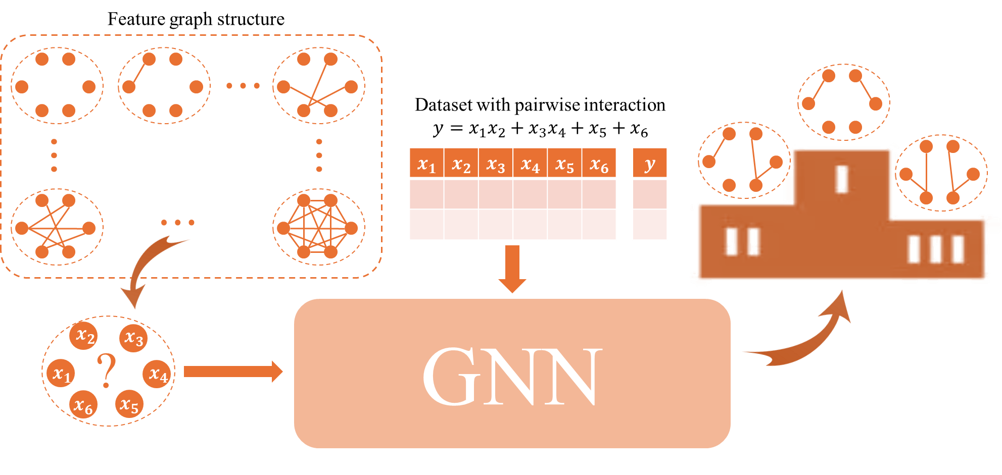
Figure 1: High-level figure to show the overall objective of our study: Given a dataset consisting of pairwise feature interaction, which structure of feature graph should we use as an input data graph structure for the given GNN model? Specifically, which graph structure can give the highest performance to GNNs? And what are the dependencies between these features that the optimal graph structure tells us?

I Introduction

Feature Interaction, one of the key challenges in predictive modeling, is the behavior of datasets whose two or more independent variables have a common influence on their dependent variable. Mathematically, it refers to operations between features in a conjunctive manner, such as multiplication, rather than treating features in isolation or through simple linear combinations. For example, if we have a dataset generated by the equation $y=x_{1}x_{2}+x_{3}$, then we say that $x_{1}$ and $x_{2}$ interact with each other in the model of $y$.

Modeling interactions can significantly improve the accuracy of predictions and reduce the complexity of models by augmenting datasets with interaction features for the models to learn from. In the best-case scenario, even linear models can be used effectively. For example, it is easier to approximate the previous function by including interaction terms $x_{1}x_{2}$ and $x_{3}$ in the dataset, rather than using more complex models with only the features $x_{1},x_{2}$ and $x_{3}$ with more complex models. Although this approach is not straightforward, it improves the interpretability of downstream tasks.

Applications of feature interaction modeling span a wide range of domains, particularly in recommendation systems, where it plays a critical role in improving predictions. The click-through rate (CTR) problem in recommendation systems is an example of an application highly based on feature interactions. For example, the age of the user and the type of product may interact in different ways on various platforms. Younger users may prefer to buy fashion products on one platform, while older users might lean towards formal products on all platforms.

Although many models, including traditional machine learning methods like decision trees, are capable of modeling feature interactions through their hierarchical structures. For example, we may consider that, in the context of meal preferences, a decision tree could represent the interaction between a type of wine and a kind of food (steak or fish) by placing the wine-related node as a descendant of the food-related node. Although this structure provides a clear representation of feature interactions, these models face significant limitations when dealing with complex or high-dimensional interactions. As the complexity of the interactions increases, the trees often become too large, leading to reduced interpretability.

Hence, we focus on graph-based methods which are more expressive in interpretability with edges between nodes. Specifically, graph-based methods represent data using graphs and model interactions through Graph Neural Networks (GNNs). Many graph-based methods have been developed to model feature interactions. Feature graphs, where nodes represent features, play an important role in GNN-based models for modeling interactions. However, a major challenge arises because most methods rely on a complete graph, where every possible interaction, i.e., every pair of features, is included. In addition, no insight and analysis about structures of feature graphs concerning features interactions are studied to make us understand the effect of graph structure to model it. One of the key questions that arises is the following: What characteristics should a feature graph have to optimally model interactions, instead of relying only on complete graphs?

Understanding the relationship between feature graph structures and their ability to model feature interactions is essential to building efficient and interpretable representations. Using a complete graph often introduces unnecessary complexity and increases computational overhead. Identifying and selectively including only the most meaningful edges in a feature graph can be considered one of the feature selection techniques for graph models that can avoid the overfitting issue.

In this work, we attempt to discover this insight, focusing on pairwise interactions, interactions between two features. We do not propose a new method; instead, we utilize existing methods in our experiments as tools for investigation. Our key contributions are as follows.

1. Theoretical Foundation for Sparse Feature Graphs: We establish a theoretical foundation for sparse feature graphs using the Minimum Description Length (MDL) principle. By framing the feature graph selection problem in the context of MDL, we prove that retaining only necessary interaction edges minimizes the description length, making it a better choice than using complete graphs. (Section V)

2. Insights into Feature Graph Structures: We provide insights into the structures of feature graphs pertaining the given feature interactions instead of using complete graphs to be used as input graphs for GNN models. Our experiment result shows that the edges corresponding to the pair of interacting features are significant and must remain in the feature graphs to maintain the prediction performance. (Section VII)

3. Empirical Validation on Real-World Datasets: We empirically show that, on real-world datasets, the feature graphs constructed by the pairwise interaction can improve the prediction performance compared with baselines including tree-based algorithms and linear-feature-based algorithms. (Section VIII)

II Preliminary

Notation	Description
$\mathbb{R}$	the set of real numbers
$\mathbb{R}^{d}$	the set of d-dimensional real-valued vector
$x$	a real feature value
$\vec{x}$	a real-valued feature vector
$G$	a graph
$V$	a set of nodes of a graph $G$
$E$	a set of edges of a graph $G$
$A$	an adjacent matrix of a graph $G$
$X$	an embedding matrix of a graph $G$
$\mathcal{N}(v)$	a set of nodes adjacent to the node $v$ in a graph $G$
$\mathcal{G}(d)$	a set of feature graphs of $d$ nodes $v_{1},\dots,v_{d}$
$v$	a node of a graph
$e_{uv}$	an edge from a node $u$ to a node $v$
$\vec{h}_{i}^{l}$	an embedding of a node $v_{i}$ in the layer $l$
$\vec{e}_{uv}$	an embedding of an edge $e_{uv}$
$\vec{m}_{i}^{l}$	a message aggregated from $\mathcal{N}(v_{i})$ in the layer $l$
$\mathcal{L}(H)$	description length for a model $H$
$\mathcal{L}(D|H)$	description length for a dataset $D$ encoded
	by a model $H$
$\mathcal{L}(D)$	minimum description length for a dataset $D$
$\mathcal{L}_{\mathbb{R}}(x)$	the number of bits of $x\in\mathbb{R}$ by some encoding

TABLE I: All related terminology

Feature Interactions

Feature interaction refers to the operation between two or more features concerning the output variable. Linear combinations or additive models represent zero-order interactions, in other words, no interaction [1]. For example, in a ground truth model, $y=5x_{1}+x_{2}x_{3}-7\sin(x_{4}-3x_{5}x_{6})$, we observe interactions between $x_{2}$ and $x_{3}$, as well as between $x_{4},x_{5}$ and $x_{6}$ with respect to $y$.

Feature Graphs and Graph Neural Networks

For graphs, we denote a tuple $G=(V,E,A,X)$ of nodes $V$, a set of edges $E$, an adjacency matrix $A$ and an embedding matrix $X$. For any node $v\in V$, we denote by $\mathcal{N}(v)$ the set of nodes adjacent to $v$, called the neighborhood of the node $v$. If only the structure of a graph is considered, we may use only $G(V,E)$.

Since we represent the interaction between features by graph edges, we model instances with the graphs whose nodes correspond to features of a dataset. According to Fi-GNN [1], this graph is called a feature graph. (see the example in Figure 2) Mathematically, given a dataset of features $x_{1},\dots,x_{d}$, a feature graph structure is a graph $G(V,E)$ where $V=\{v_{1},\dots,v_{d}\}$.

There are many tools that can be used to process graphs. Among these GNN models have gained significant attention due to their effectiveness in handling complex, non-Euclidean data. GNNs are a category of neural models specifically designed to operate on graph data structures, where the order of nodes should not influence the computation of predicted values, a property referred to as “permutation invariance.” There are various approaches to implement GNNs, but one of the most prominent paradigms is based on “message passing.”

In our context, message passing can be described through the following equations:

$$\vec{m}_{i}^{(k)} =\bigoplus_{j\in\mathcal{N}(i)}\phi^{(k)}\left(\vec{h}_{i}^{(k-1)},\vec{h}_{j}^{(k-1)},\vec{e}_{j,i}\right)$$ (1)

$$\vec{h}_{i}^{(k)} =\gamma^{(k)}\left(\vec{h}_{i}^{(k-1)},\vec{m}_{i}^{(k-1)}\right)$$ (2)

where $\bigoplus$ represent a differentiable, permutation-invariant function, such as summation, averaging, or maximum operation, while $\gamma$ and $\phi$ denote differentiable functions, often implemented as neural network layers. In Equation 2, the model updates the node information using both existing information (from the previous layer) and information shared among neighboring nodes (messages), which is computed as Equation 1. The latter equation pertains to the aggregation of messages from neighboring nodes.

Message passing layers are not the sole focus in GNN models; pooling layers also play a crucial role, particularly in tasks like graph classification. Pooling involves summarizing local information in a graph, such as node embeddings, to derive a global representation of the entire graph. There are various methods for graph pooling, including sum pooling and mean pooling [2].

Minimum Description Length (MDL)

Our problem can be framed as the selection of models, specifically the representation of graphs. MDL [3, 4] is a paradigm of model selection that attempts to find the model that minimizes the number of bits that represent information. This information may include the complexity of models and the performance score of the model on given data.

In our work, we use MDL to study the model whose complexity is minimized while maintaining the well-performed accuracy of the prediction. It is the two-stage code description approach [5]. Specifically, it encodes the data $D$ with the description length $\mathcal{L}_{\mathcal{H}}(D)$ by first encoding a hypothesis $H$ from the set of given hypotheses $\mathcal{H}$ followed by encoding $D$ with the help of $H$. The objective is to minimize the total description length as follows:

$$\mathcal{L}_{\mathcal{H}}(D):=\min_{H\in\mathcal{H}}(\mathcal{L}(H)+\mathcal{L}(D|H)).$$

In other words, $\mathcal{L}(H)$ includes any descriptions related to the model, such as coefficients in linear regression or the number of edges in the representation of the feature graph (as used in this work). The latter term, $\mathcal{L}(D|H)$, typically includes the code length of the prediction errors and the code length of the data.

III Related Work

III-A Feature Interaction Modeling

Feature interactions in terms of nonadditive terms play a crucial role in model-based predictive modeling. Many works attempted to develop methods to indicate the interaction. Beginning with the statistical-based measure called Friedman’s H statistic [6] involving the theory of partial dependency decomposition. However, it is computationally expensive and is dependent on predictive models.

From the perspective of machine learning, many models were proposed to model feature interactions, especially variants of factorization models inspired by FM [7]. FM relies on the inner product between the embedding of the feature-value motivated by the factorization of matrices. Several variants of FM have been proposed to fill the gaps. FFM [8] takes into account the embedding of feature field (i.e. columns in a table of data). AFM [9] considers the weight of the interaction by adding attention coefficients to its model.

The success of deep nets in various domains motivates researchers to use them in modeling interactions. For example, Factorization Machine supported Neural Network (FNN) [10] proposed a deep net architecture that can automatically learn effective patterns from categorical feature interactions in CTR tasks. In addition, DeepFM [11] proposed a kind of similar idea but included a special deep net layer that performs the FM task.

The attention mechanisms [12] are the method designed to model the importance between different components. In AFM, the attention mechanism was applied because the authors believe that all interactions should not be treated equally likely with respect to prediction values. Attention allows the model to weight feature interactions differently based on their importance. After introducing the attention mechanism to interaction tasks, many works use attention to model the interaction of features based on the factorization machine framework [13, 14, 15, 16, 17].

One of the crucial challenges of interactions in traditional machine learning models is the explainability of which features have interaction, although some of them outperform in prediction performance. So we need an explicit representation that can correspond to pairwise interaction, where a graph is a representation that can fill this gap. In addition, GNN is a tool that can be used to learn information from graphs.

III-B Graph Neural Networks for Feature Interactions

GNN are becoming more interesting for use in feature interaction problems. Since feature interactions can be seen as relationships between features, most of the works rely on feature graphs for each individual instance to represent the interactions via aggregation of representation from neighbor nodes.

Motivated by the click-through rate (CTR) prediction, which is believed to influence the rate of clicking on a product, such as age and gender, many works attempted to model this prediction by using GNN applied feature graphs. To the best of our knowledge, Fi-GNN [1] is the first work to use GNN to model the interaction of features in the feature graph for the prediction of CTR. It applied the field-aware embedding layer to compute the latent representation of nodes of features before feeding the feature graph with the computed representations into a stack of message passing layers.

After the introduction of Fi-GNN, many subsequent works have built on this idea. Cross-GCN [18] used a simple graph convolutional network with cross-feature transformation. GraphFM [19] seamlessly combined the idea of FM and GNN using the neural matrix factorization [20] based function to estimate the edge weight. It also adopts the attentional aggregation strategy to compute feature representation. Table2Graph [21] applied attention mechanisms to compute the probability adjacency matrix instead of edge weight. It also used the reinforcement learning policy to capture key feature interactions by sampling the edges within feature graphs.

All mentioned works chronically improve the methods of feature interaction learning. However, no work provides information about the effect of the construction of feature graphs on the learning capacity. Most of the works utilize attention mechanisms or edge weights to let models learn graph structures via these parameters.

IV Problem Formulation: Pairwise Interaction Feature Graph Problem

An important open research question in graph representation for data without explicit connections is that What is a suitable graph structure? While current research highlighted the potential of feature graphs, a feature graph that is too dense, for example, a complete graph, may lead to learning issues, as shown and discussed in previous work [1, 22, 23] and in Section VII-E. Thus, finding an optimal feature graph structure for any particular prediction task is the common goal of the community. Consequently, we can formulate the “feature-graph-finding” problem as follows:

$$G^{*}=\operatorname*{arg\,min}_{G\in\mathcal{G}(n)}\ell(\vec{y},\text{GNN}(X;G)),$$

where $\text{GNN}(\ \cdot\ ;G)$ is a given GNN model trained for the feature graph $G$, and $\ell$ is an arbitrary but fixed loss function for the prediction task. The above task is not traceable as there are exponentially many possible graph structures ($\mathcal{O}(2^{n^{2}})$.) Many works attempted to solve this problem using soft learnable interactions [1, 19] or hard interactions through reinforcement learning [21]. However, they did not provide any insight into the characteristics of a suitable feature graph structure related to the interaction between features.

Consequently, instead of solving the “feature-graph-finding” problem, this work aims to study the relationship between feature graph structures and their performance in modeling feature interactions. Specifically, we would like to theoretically show that (1) feature graphs correspond to feature interactions and (2) keeping only edges between interacting feature nodes is sufficient under MDL assumptions.

V Theoretical Results

There are two questions that we should address. The first is “Is the space of the functions and the space of feature graphs a correspondence?” It is significant because we aim to guarantee that we can use some graph to represent any of the given functions and vice versa. The second question is that of “Why do we need sparse graphs rather than complete graphs?” Here, we consider the second problem to be the problem of model selection according to the concept of MDL. Proofs of results in this section are in the Appendix.

V-A Correspondence Problem

It is worth considering the correspondence between expressions and graph structures. Even though we primarily focus on pairwise interactions, in this correspondence, we go towards the arbitrary number of variables interacting, not only pairwise. For convenience of stating, we discuss only the multiplicative interactions, which is a special case of the non-additive interaction. Throughout this, let us call the kind of expression disjoint multilinear interaction which is defined as follows:

Definition 1 (Disjoint Multilinear Interaction Expression).

The predictive model $y(\vec{x})$ is said to be a disjoint multilinear interaction expression (DMIE) if it can be expressed as

$$y(\vec{x})=\sum_{i=1}^{n}\prod_{j=1}^{m_{i}}x_{i_{j}}$$ (3)

where $x_{i_{j}}$ and $x_{k_{l}}$ are distinct variables when $i\neq k$ or $j\neq l$. We denote by $\mathcal{DM}(n)$ the set of all DMIE expressions of $n$ variables.

Multiple graphs can infer the same expression considering the perspective of connected components. For example, the expression $x_{0}x_{1}x_{2}+x_{3}x_{4}+x_{5}+x_{6}$ corresponds to the graphs $E_{1}=\{\{0,1\},\{0,2\},\{1,2\},\{3,4\}\}$ and also $E_{2}=\{\{0,1\},\{1,2\},\{3,4\}\}$. Consequently, we use equivalence classes of graphs (based on connectedness) instead of individual graphs. To this end, we define an equivalence class of feature graphs.

Definition 2.

We define a binary relation $\sim$ in $\mathcal{G}(n)$ as follows: for any graph $G_{1},G_{2}\in\mathcal{G}(n)$, $G_{1}\sim G_{2}$ if for any $i,j\in N_{n}$, they are reachable in $G_{1}$ if and only if they are reachable in $G_{2}$.

Obviously, $\sim$ is an equivalence relation to $\mathcal{G}(n)$. We then denote the set of equivalence classes from $(\mathcal{G}(n),\sim)$ by $\mathfrak{G}(n)$:

$$\mathfrak{G}(n):=\left\{\left[G\right]_{\sim}:G\in\mathcal{G}(n)\right\}$$ (4)

As a result, we can prove the correspondence, as presented in Theorem 3.

Theorem 3.

$\mathcal{DM}(n)$ one-to-one corresponds to $\mathfrak{G}(n)$.

V-B MDL for graph representation of pairwise interaction

This problem can be considered as a model selection problem for selection of representations. We adopt the idea of Minimum Description Length (MDL) to shape the problem in the manner of selection of graph representation. Generally speaking, a selected feature graph should not be so dense that it captures an uninformative characteristic. On the other hand, it should not be such a light graph that the informative edges to learn interactions are omitted. In this work, we focus on the pairwise interaction case, which is formalized below.

Given a graph $G=(V,E)$ whose nodes are of degree at most 1, a function containing pairwise interaction induced from $G$ is defined as

$$f_{G}(x)=\sum_{\deg(i)=0}c_{i}x_{i}+\sum_{\{i,j\}\in E}c_{ij}x_{i}x_{j}$$ (5)

Note that we represent pairwise interaction by bilinear interaction for convenience in describing by mathematical notation. Therefore, the problem of selecting the graph for this function $f_{G}$ is framed as Problem 1.

Problem 1 MDL Pairwise Interaction Graph Problem******

Input: A dataset $\mathcal{S}=\{(x_{i},y_{i})\}_{i=1}^{n}$, and a pre-configured GNN model $\mathcal{F}:\mathfrak{G}\times\mathbb{R}^{d}\to\mathbb{R}$
Output: The edge set $E^{*}$ for an input feature graph $G^{*}(V,E^{*})\in\mathfrak{G}$ so that

$$G^{*}=\operatorname*{arg\,min}_{G\in\mathfrak{G}}{\mathcal{L}(f_{G})+\mathcal{L}(S|f_{G})}$$ (6)

In this problem, we denote $\mathcal{L}(S,f_{G})=\mathcal{L}(S|f_{G})+\mathcal{L}(f_{G})$, where

$$\mathcal{L}(f_{G}) =\mathcal{L}_{\mathbb{R}}(|E(G)|)+\sum_{\deg(i)=0}\mathcal{L}_{\mathbb{R}}(c_{i})+\sum_{\{i,j\}\in E(G)}\mathcal{L}_{\mathbb{R}}(c_{ij})$$ (7)

$$\mathcal{L}(S|f_{G}) =\sum_{i=1}^{n}\mathcal{L}_{\mathbb{R}}(x_{i})+\sum_{i=1}^{n}\mathcal{L}_{\mathbb{R}}(y_{i}-f_{G}(x_{i}))$$ (8)

We denote by $\mathcal{L}_{\mathbb{R}}:\mathbb{R}\to\mathbb{N}$ a function of the number of bits $\mathcal{L}_{\mathbb{R}}(x)$ we need to encode a real number $x$. In the next part, we will show that the description length of the optimal graph $G^{*}$ is bounded by the lengths of both the complete graph $K$ and the null graph $N$.

Assumptions

Our consequent result in this paper is based on these assumptions about $\mathcal{L}_{\mathbb{R}}$:

1. $\forall x_{1},x_{2}\in\mathbb{R},\mathcal{L}_{\mathbb{R}}(x_{1}+x_{2})\leq\mathcal{L}_{\mathbb{R}}(x_{1})+\mathcal{L}_{\mathbb{R}}(x_{2})$

2. $\forall x_{1},x_{2}\in\mathbb{R},|x_{1}|\leq|x_{2}|\iff\mathcal{L}_{\mathbb{R}}(x_{1})\leq\mathcal{L}_{\mathbb{R}}(x_{2})$

3. $\exists D>0\forall x,y\in\mathbb{R},|x-y|\leq 1\Rightarrow|\mathcal{L}_{\mathbb{R}}(x)-\mathcal{L}_{\mathbb{R}}(y)|\leq D$

We assume that the functions that generate $Y$ from $X$ in a dataset, denoted by $S_{G^{*}}:=\{(X_{i},Y_{i})\}_{i=1}^{n}$, are induced by some feature graph $G^{*}$ as Equation 5, i.e.

$$Y=f_{G^{*}}(X)+\mathcal{E}$$

where $\mathcal{E}$ is a noise random variable from some truncated distribution, i.e. there exists $\epsilon^{*}>0$ with $|\mathcal{E}|\leq\epsilon^{*}$.

We also denote $\hat{f}_{G}$ a function $f_{G}$ corresponding to a feature graph $G$ whose parameters are approximated by $S_{G^{*}}$. Moreover, we assume that the parameters of actual additive terms can be learned well (by some learning algorithm). Specifically, if the term $c_{i}x_{i}$ exists in the ground truth function, then the parameters $d_{i}$ of the feature graph can be learned so that $\mathcal{L}_{\mathbb{R}}(d_{i}-c_{i})\approx 0$. It is similar for the interaction term $c_{ij}x_{i}x_{j}$, the parameter $d_{ij}$ can be learned so that $\mathcal{L}_{\mathbb{R}}(d_{ij}-c_{ij})\approx 0$.

We also assume further that if the features $a$ and $b$ interact with each other in the expression of ground truth, then $\mathcal{L}_{\mathbb{R}}(\hat{d}_{a})+\mathcal{L}_{\mathbb{R}}(\hat{d}_{b})>>\mathcal{L}_{\mathbb{R}}(\hat{c}_{ab})$ where $\hat{d}_{a}$ and $\hat{d}_{b}$ are the coefficients learned by the expression that these features are additive and $\hat{c}_{ab}$ are those learned by the expression consisting of the interaction term between $x_{a}$ and $x_{b}$. So, it is safe to assume that $\mathcal{L}_{\mathbb{R}}(\hat{d}_{a})+\mathcal{L}_{\mathbb{R}}(\hat{d}_{b})-\mathcal{L}_{\mathbb{R}}(\hat{c}_{ab})\geq D$ which is a uniform bound of difference between two real numbers that is not further than 1. On the other hand, we also assume that if $a$ and $b$ do not interact with each other, then $\mathcal{L}_{\mathbb{R}}(\hat{c}_{ab})>>\mathcal{L}_{\mathbb{R}}(\hat{d}_{a})+\mathcal{L}_{\mathbb{R}}(\hat{d}_{b})$.

For the description length of error term $\sum_{i=1}^{n}\mathcal{L}_{\mathbb{R}}(y_{i}-f_{G}(x_{i}))$, we need the assumption that fitting a pairwise interaction term $c_{ab}x_{a}x_{b}$ by the additive terms $c_{a}x_{a}+c_{b}x_{b}$ always yields dramatic length with respect to the noise term $\epsilon_{i}$ so that

$$\mathcal{L}_{\mathbb{R}}(c_{ab}x_{a}x_{b}-(\hat{c}_{a}x_{a}+\hat{c}_{b}x_{b})+\epsilon_{i})>>\mathcal{L}_{\mathbb{R}}(\epsilon_{i}).$$

Similarly, we also need a similar assumption to fit the additive terms $c_{a}x_{a}+c_{b}x_{b}$ by the interaction term $c_{ab}x_{a}x_{b}$ as follows:

$$\mathcal{L}_{\mathbb{R}}((c_{a}x_{a}+c_{b}x_{b})-\hat{d}_{ab}x_{a}x_{b}+\epsilon_{i})>>\mathcal{L}_{\mathbb{R}}(\epsilon_{i}).$$

First, we begin with the most intuitive result motivated by our empirical result that we must keep the edges of interactions and we should prune non-interaction edges out in the desired feature graph.

Lemma 4.

If $\{a,b\}\in E(G^{*})$, then we have

$$\sum_{i=1}^{n}\mathcal{L}_{\mathbb{R}}(y_{i}-f_{G^{*}\setminus\{a,b\}}(x_{i}))\geq\sum_{i=1}^{n}\mathcal{L}_{\mathbb{R}}(y_{i}-f_{G^{*}}(x_{i})).$$

If $\{a,b\}\notin E(G^{*})$, then

$$\sum_{i=1}^{n}\mathcal{L}_{\mathbb{R}}(y_{i}-f_{G^{*}\cup\{a,b\}}(x_{i}))\geq\sum_{i=1}^{n}\mathcal{L}_{\mathbb{R}}(y_{i}-f_{G^{*}}(x_{i})).$$

Proposition 5.

If $\{a,b\}\in E(G^{*})$, then we have $\mathcal{L}(S_{G^{*}},f_{G^{*}\setminus\{a,b\}})\geq\mathcal{L}(S_{G^{*}},f_{G^{*}})$. On the other hand, if $\{a,b\}\notin E(G^{*})$, then $\mathcal{L}(S,f_{G^{*}\cup\{a,b\}})\geq\mathcal{L}(S_{G^{*}},f_{G^{*}})$.

By Lemma 4, it is easy to show that:

Corollary 6.

Let $K$ be the complete feature graph of the features of $S_{G^{*}}$. Then

$$\sum_{i=1}^{n}\mathcal{L}_{\mathbb{R}}(y_{i}-\hat{f}_{K}(x_{i}))\geq\sum_{i=1}^{n}\mathcal{L}_{\mathbb{R}}(y_{i}-\hat{f}_{G^{*}}(x_{i}))$$

Consequently, we obtain the desired result.

$$\mathcal{L}(S_{G^{*}},f_{G^{*}})\leq\mathcal{L}(S_{G^{*}},f_{K}).$$

Not only for the complete graph, but also for the graph without edges we aim a similar result.

Corollary 7.

Let $N$ be the feature graph without edges. Then

$$\sum_{i=1}^{n}\mathcal{L}_{\mathbb{R}}(y_{i}-\hat{f}_{N}(x_{i}))\geq\sum_{i=1}^{n}\mathcal{L}_{\mathbb{R}}(y_{i}-\hat{f}_{G^{*}}(x_{i}))$$

Hence, we also have $\mathcal{L}(S_{G^{*}},f_{G^{*}})\leq\mathcal{L}(S_{G^{*}},f_{N})$.

Theorem 8.

For any feature graph $G$ containing all interaction edges, we have

$$\mathcal{L}(S_{G^{*}},f_{G})\leq\mathcal{L}(S_{G^{*}},f_{K})$$

$$\mathcal{L}(S_{G^{*}},f_{G})\leq\mathcal{L}(S_{G^{*}},f_{N})$$

Implication

The theoretical results shown in Section V-A are just to ensure us that we can confide in learning feature graph structures to infer an expression containing feature interactions. In other words, given any function containing feature interactions of at most one occurrence for each feature, there always exist feature graph structures that can infer backward to the function and vice versa. Therefore, to find such graph structures, we need some insight into graph construction related to feature interactions.

Consequently, we reformulate these observations into more general arguments. Generally speaking from empirical results in Section VII-B, it is better to maintain all the edges of the interaction in the feature graph to maximize the learning interaction in a given dataset. Also, it is better to prune non-interaction edges out as much as possible to avoid fitting noise information. Finally, these results are supported by Proposition 5.

In addition, we also show the empirical result about using complete feature graphs to learn from larger datasets in Subsection VII-E. Although the result in Subsection VII-B cannot infer the limitation of complete graph obviously, the result in Subsection VII-E reveals that the complete feature graphs are worse when datasets are larger in feature size. Finally, we can show that, in the manner of MDL which is a framework of model selection, the complete feature graph is worse than any feature graphs containing all interaction edges. This tells us that it is not a good idea to use the complete feature graph to learn from datasets. Not only learning hidden noise, but it also face with the computation and memory issues. In the next section, we will focus on the empirical results in more details.

VI Methodology

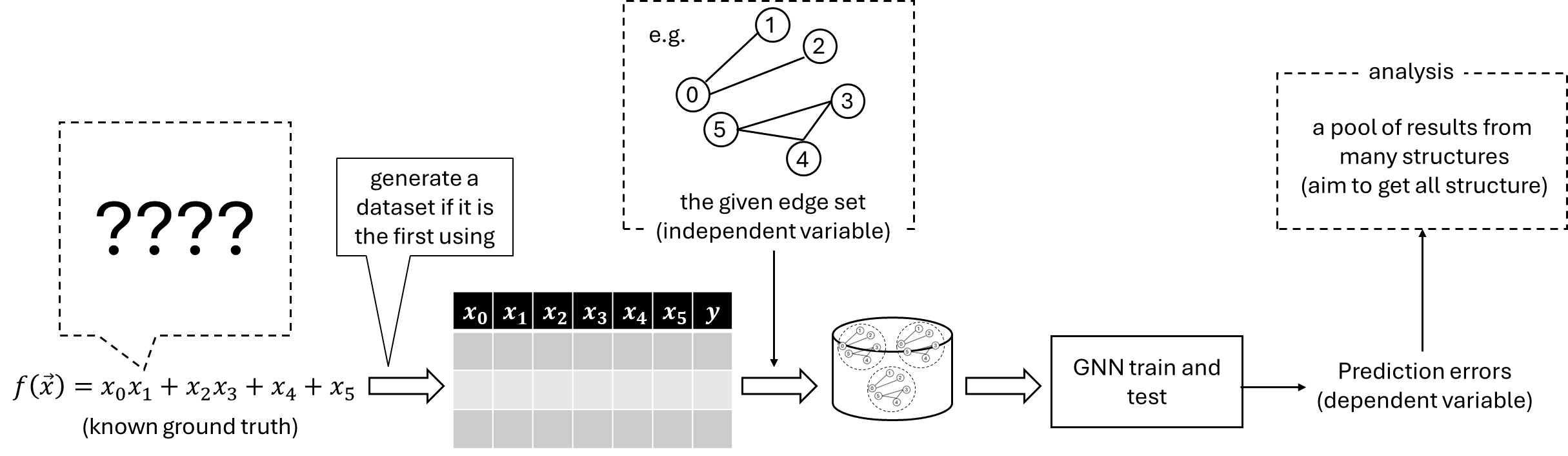
Figure 2: Experimental procedure: data generation based on a ground truth function and variation of feature graph structures as an input.

Our experiment provides empirical evidence regarding the relationship between feature graph structures and pairwise interactions in datasets. We train and evaluate several feature graph structures for each dataset and report the results. However, due to the combinatorial number of possible feature graph structures and the stochastic nature of the learning algorithm, we adopt a strategy of generating random edge sets to explore various graph configurations, as illustrated in Figure 2.

VI-A Datasets

Real-world datasets rarely provide information about interactions between features, which disables our analysis. To this end, we use synthesized datasets to control interaction characteristics in datasets such as the number of interaction pairs of features, strength of interactions, or kinds of interactions. We assume that there is only one mode of interaction per feature graph. If real-world datasets had many interaction modes, we could apply weighted ensemble feature graphs proposed Li et al. [17]

Construction of the simulated dataset (the first arrow in Figure 2) can be formally described as follows. Let $f:\mathbb{R}^{d}\to\mathbb{R}$ be a hidden ground truth function containing pairwise interaction terms. A synthetic dataset of $n$ instances with respect to $f$ if $\{(\vec{X_{i}},f(\vec{X_{i}})+0.1\mathcal{E}_{i})\}_{i=1}^{n}$ where $\vec{X_{i}}\sim\mathcal{N}(0,1)$ and $\mathcal{E}_{i}\sim\mathcal{N}(0,\text{var}(f(\vec{X_{i}})))$. We varied the number of features and interaction pairs to aid our analyses. Note that for each function $f$, we generated one set of data and used it for all variations of feature graphs.

VI-B Feature graphs

For a given function $y=f(x_{1},x_{2},\dots,x_{d})$ of $d$ features, a set of feature graphs is constructed by randomly assigning edges between feature nodes (see Figure 2 after the second arrow). In other words, given a dataset of $d$ features and $n$ samples $\{(\vec{x}_{i},y_{i})\}_{i=1}^{n}$ and an edge set $E$ for a graph of $d$ nodes, the feature graph dataset of edge set $E$ is a graph dataset $\left\{(G(V,E,\text{concat}(\vec{x},X)),y_{i})\right\}_{i=1}^{n},$ where $X$ is a learnable embedding for a feature graph for nodes. The initial node embedding matrix is denoted by

$$H^{(0)}=\text{concat}(\vec{x},X).$$ (9)

VI-C GNN Architectures

Our GNN model utilizes transformer convolution layers (TransformerConv [24]) for the message passing function, incorporating attention mechanisms to capture the strength of pairwise interactions, as depicted in Figure 3. Then, a mean pooling layer averages the embedding of all nodes for the prediction layer.

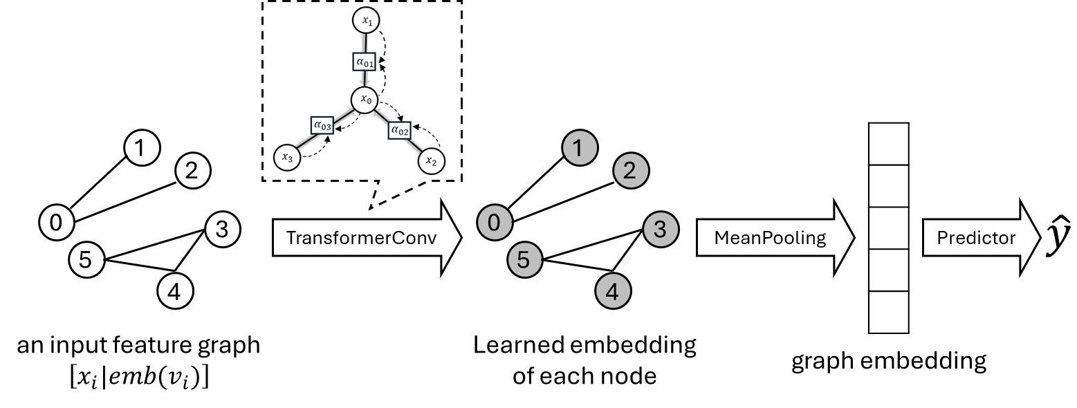
Figure 3: (will be fixed for used notation) Detail of the GNN model: from feature graph construction to output prediction.

As Fi-GNN does, this work adopts the idea from Fi-GNN, but simpler architecture. We use TransformerConv [24] which is a message-passing layer based on the attention mechanism whose feature interaction learning capability is shown by many works. For the computation, we start from the initial node embedding $H^{(0)}$ defined in Equation 9. Then a feature graph with the node embedding matrix is fed to TransformerConv with BatchNorm:

$$\begin{split}Z^{(l)}&=\text{TransformerConv}(H^{(l-1)},E),\\ H^{(l)}&=\text{ReLU}(\text{BatchNorm}(Z^{(l)})),\end{split}$$ (10)

where $H^{(l)}$ is an intermediate node embedding matrix at the layer $l$. After applying all message passing layers, we calculate the average pooling of node embeddings from the last GNN layer, and we use this vector as a graph embedding which is fed into the projection layer to get prediction:

$$\vec{p} =\frac{1}{n}\sum_{i}H^{(L)}[i],$$ (11)

$$\hat{y} =\vec{w}\cdot\vec{p}+b,$$ (12)

where $H^{(L)}$ is a node embedding matrix from the last GNN layer and $H^{(L)}[i]$ is the row $i$ of the matrix which corresponds to the node embedding of the node $i$ and $b$ is a biased term. Equation 11 is the calculation of mean pooling layer and Equation 12 is the final projection to calculate the prediction value.

Equation 10 is a bit different from the original work [24] which uses LayerNorm after aggregation of message like as the original transformer in NLP. In the first phase of experiment, we found that the GNN model with LayerNorm cannot capture interaction behavior while BatchNorm can.

In training the GNN model, we adopt an usual supervised learning approach, where the loss function measures the difference between the predicted value, $\hat{y}$, and the true target value, $y$. Specifically, we use the mean squared error (MSE) loss, which is defined as

$$\mathcal{L}_{\text{MSE}}=\frac{1}{N}\sum_{i=1}^{N}(\hat{y}_{i}-y_{i})^{2},$$

where $N$ is the number of samples.

VII Experiments and Results

Results shown in this section are from the dataset generated by the equation $f(\vec{x})=\sum_{i=1}^{p}x_{2i-1}x_{2i}+\sum_{i=1}^{q}x_{2p+i}+\epsilon$. We present the experiment results in the following insights:

1. The efficient structures of feature graphs (Section VII-B)

2. The dependency between edges and interaction pairs (Section VII-C)

3. The relationship between multi-hops and number of message passing layers (Section VII-D)

4. Scalability of efficient feature graphs (Section VII-E)

Since Section VII-B - VII-D consider the variants of graph structures w.r.t. the given dataset, we show only results from an equation containing 2 interaction terms and 2 unary terms, i.e. $p=2,q=2$. In Section VII-E, $p$ is varied while $q=2$.

VII-A Experimental Setting

Synthetic dataset generating

Each synthetic dataset contains 10,000 samples generated by distribution described in Methodology section (Section VI). In every randomization, we use seed number $n$ for feature $x_{n}$ and seed number 0 for noise term. We split it into first 7,000 rows for training and next 3,000 rows for testing sets.

Random sampling of feature graph structures

Ideally, we want results of all possible feature graph structures. However, there are up to $\mathcal{O}(2^{n^{2}})$ feature graphs for a dataset of $n$ features. This leads us to the combinatorial issue, so we set up an experiment by sampling in random stratified by (1) the number of edges, (2) the number of interaction edges, (3) the number of non-interaction edges, and (4) the number of hops between interacting nodes. Since we also want to study about subgraphs with respect to existence of interaction edges (for example, edges $\{0,1\}$ and $\{2,3\}$ for the dataset generated by $y=x_{0}x_{1}+x_{2}x_{3}+x_{4}+x_{5}$), we want these collections (1) graphs having both edges, (2) graphs having $\{0,1\}$ but not $\{2,3\}$ (3) vice versa and (4) graphs having no these edges. To have full collections to compare, once any feature graph is sampled, all other three graphs are also sampled.

Model setting and training

We also vary the number of message passing layers from 1 layer to 3 layers where all models’ hyperparameters are set to have the equally likely number of parameters. In all setting, we use the 16-dimensional node embedding $X$. The hidden size in TransformerConv $H^{(i)}$ for 1, 2 and 3 MP layers is 26, 20, and 16, respectively. In training of models, we use Adam optimizer with automatically schedule of learning rate.

VII-B Interaction Edges vs. Non-interaction Edges

We are first interested in the existence of interaction edges and that of non-interaction edges. Intuitively, the existence of interaction edges should be significant for learning the interaction between features by attention-based GNNs since they allow paasing of the message between their associated nodes to model interactions.

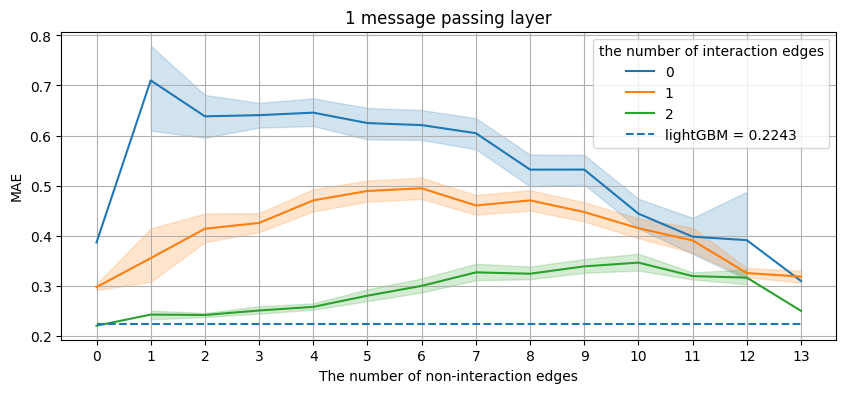
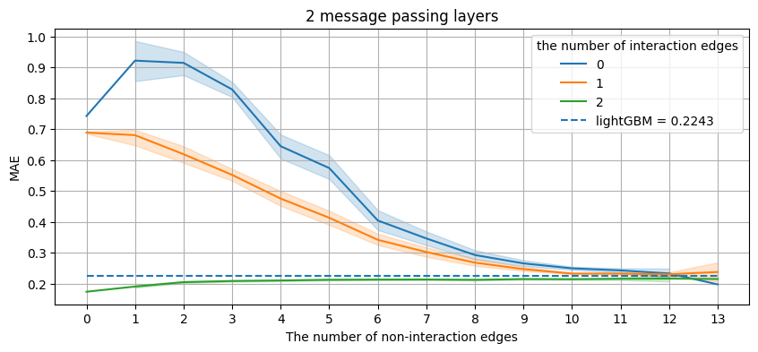
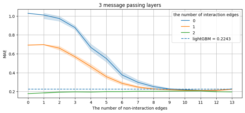
Figure 4: the average of MAE (y-axis) in prediction against the number of non-interaction edges (the edges corresponding to the nodes of features not interacting in equation, e.g. the edge $\{0,4\}$ or the edge $\{4,5\}$) in x-axis where different lines in the same figure indicated by color are for the number of interaction edges (there are two possible interaction edges in this equation: $\{0,1\}$ and $\{2,3\}$)

Figure 4 illustrates the average MAE in predicting each number of edges without interaction along the $x$ axis. Each line corresponds to the number of interaction edges. We see that among the graphs that have the same number of non-interaction, feature graphs containing all interaction edges give significantly lower errors than the graphs missing some interaction edges give for all of the number of non-interaction edges. Especially, we also see that even though graphs with all interaction edges contain any number of other noise edges, they still give good performance compared to the entire line of the graphs missing some interaction edges. From this result, we may infer that the interaction edges are the most important in input feature graphs to learn a dataset containing pairwise interaction. Although we do not know how to construct feature graphs used by GNN models for the task that we believe that there must be interaction terms, at least the interaction edges (if we know) should be kept.

This result also tells us that when the feature graph can maintain all interaction edges, the increasing number of non-interaction edges leads to poorer performance. It seems that the non-interaction edges make a model capture non-underlying information in a dataset and interfere with the learning of pairwise interactions of interaction edges.

However, if we consider the results of the 0-interaction-edge and 1-interaction-edge graphs, we notice a different trend from the 2-interaction-edge graphs. It starts with the worst result when there are no edges in a graph. In this case, the more noninteraction edges it has, the better the performance. One hypothesis of us at first sight is that the more number of edges (even though they are not interaction edges), the higher chance that interaction nodes can pass messages in GNNs’ computation via multi-hop connectivity rather than direct interaction edges. This leads us to consider the connectivity of interacting nodes rather than the direct edges between them.

VII-C Removing Interaction Edges from a Graph

The above figure shows the result in average. However, the information about subgraphs is not shown in them, while it is another interesting property that can motivate us to construct an appropriate feature graph. For the subgraph property, we consider the effect of removing the interaction edge from a graph. For example, if we consider a graph $G$ containing all interaction edges, i.e. $\{\{0,1\},\{2,3\}\}\subseteq E(G)$ w.r.t. $x_{0}x_{1}+x_{2}x_{3}+x_{4}+x_{5}$, the other considered subgraphs compared to this graph are $E(G)\setminus\{\{0,1\},\{2,3\}\}$, $E(G)\setminus\{\{0,1\}\}$ and $E(G)\setminus\{\{2,3\}\}$. Figure 5 shows an abstract lattice of the subgraphs. Our claim is that the performance would drop along this lattice from top to bottom of lattice.

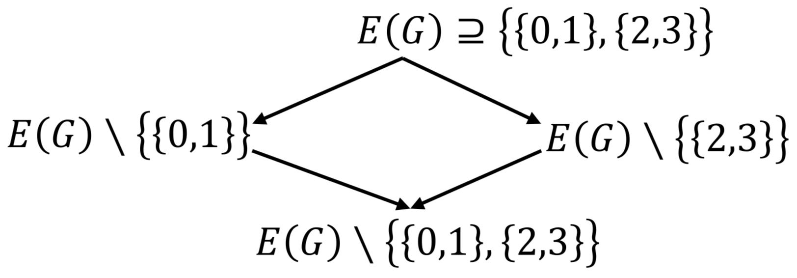
Figure 5: a lattice of subgraph of a given graph $G$ containing all interaction edges for $x_{0}x_{1}+x_{2}x_{3}+x_{4}+x_{5}$

To this end, we perform a statistical analysis by the confidence interval of the paired difference of MAE where the pair of graphs is paired with the subgraphs by removing the interaction edges: $\text{MAE}(G\setminus\{a,b\})>\text{MAE}(G)$ where an edge $\{a,b\}$ is an interaction edge in a graph $G$.

The lower-sided confidence interval 95% is shown in Table II. It ensures us that interaction edges are significantly important for input feature graph in attention-based GNNs. Figure 6 shows the MAE of some random sample generated, sorted by the MAE of $E(G)\setminus\{\{0,1\},\{2,3\}\}$ from the 3 message passing layer model to illustrate how they are.

graph	dropped	1MP	2 MPs	3 MPs
$G$	$\{0,1\}$	$>0.124$	$>0.173$	$>0.160$
$G$	$\{2,3\}$	$>0.129$	$>0.186$	$>0.163$
$G\setminus\{0,1\}$	$\{2,3\}$	$>0.114$	$>0.132$	$>0.137$
$G\setminus\{2,3\}$	$\{0,1\}$	$>0.114$	$>0.156$	$>0.166$

TABLE II: 95% lower-sided confidence interval of paired-difference of MAE between a graph and interaction-edge-removed graph

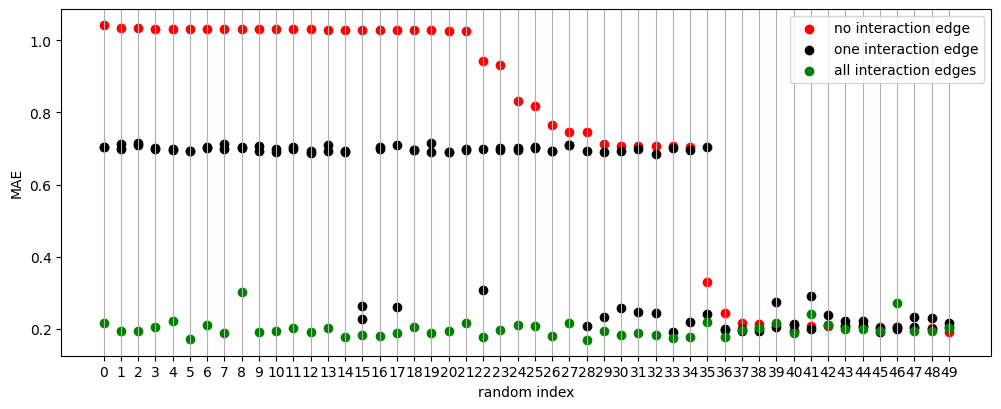
Figure 6: Samples of MAE score colored by the number of interaction edges and sorted by in x-axis by MAE of no-interaction-edge graphs to show the increasing of MAE when an interaction edge is removed, where our $G$ in this subsection corresponds to the green points

VII-D Reachability of Interaction Nodes and the Number of Message Passing Layers through a Longer Path

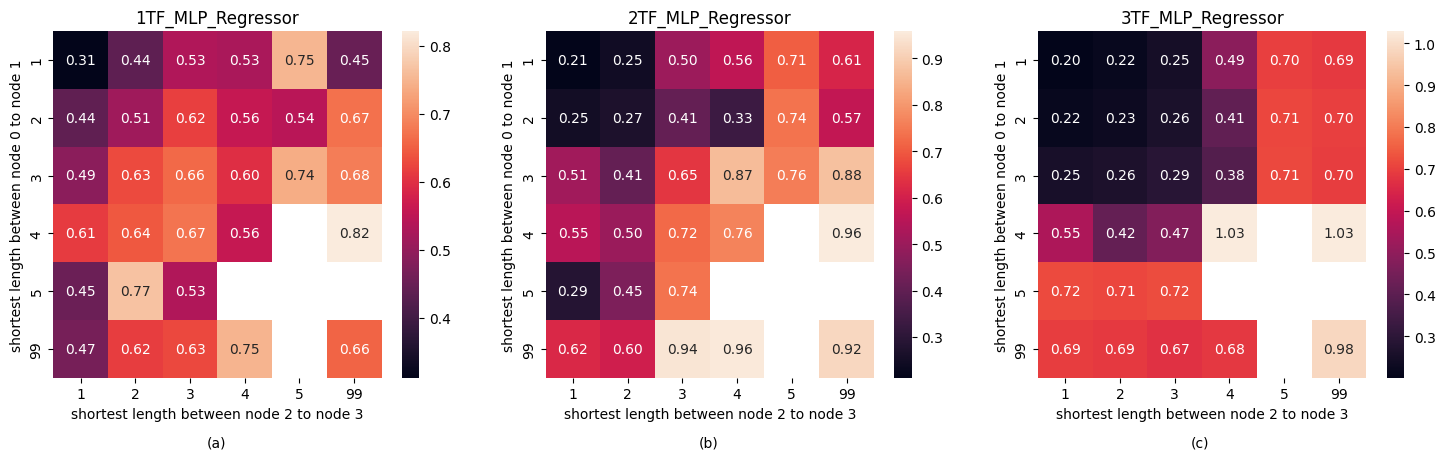
Figure 7: Heatmap of average MAE for the number of hops between interaction nodes (between node 0 and node 1 in vertical and between node 2 and node 3 in horizontal) for a model consists of (a) 1 MP layer, (b) 2 MP layers and (c) 3 MP layers: 99 means not reachable

In the previous result, we discussed the effect of the occurrence and absence of interaction and noninteraction edges. We observed that the feature graphs without interaction edges can predict the test set better with the help of increasing non-interaction edges. So, it comes up with the question about connectivity whether GNN models can capture interaction patterns via paths, not necessarily to be adjacent, and whether the length of a shortest path relates or not.

In Figure 7 (a), we see that although the interacting nodes are not adjacent, these graphs can still be used at some level if they are reachable. In other words, connectivity through a sufficient number of hops can also yield satisfactory results.

We also see that the longer the shortest path between interacting nodes, the worse the score. This result shows a considerable increase in error when the number of hops increases from 1 hop to 2 hops in both directions. This might be because we used only one message passing layer in the model. This allows the passing of messages between nodes only for one hop.

Since the passing message allows nodes to exchange their messages via edges, the greater number of layers should allow further nodes to do so. So we show, in Figure 7 (b)-(c), an alternative result experiment in which a GNN model consists of 2 and 3 message passing layers whose hyperparameters are set to have the same number of parameters as that of the 1-layer model. The result is analyzed similarly to that shown in Figure 7 (a).

In Figure 7 (b) compared to (a), we see that the 2-layer model can be trained using a feature graph to ensure that the interaction nodes are reachable to each other up to 2 hops. Similarly, Figure 7 (c) of a 3-layer GNN reveals that the feature graph of up to 3 hops of interaction nodes can be used to train the GNN model. This may infer that the more messages that pass through, the weaker the condition of reachability of the interaction node.

VII-E Limitation of Complete Feature Graphs

From the result in Figure 4, the complete feature graph can give errors almost similar to that of the graph that contains only interacting edges. This may sound like a good result to tell us that it is not necessary to find the optimal graph structures. However, the demonstrating dataset is very small in number of features. It contains only 6 features; then the complete graph consists of only 15 edges, which is small. Therefore, we ask the question of how it will be when datasets contain more and more features.

a result from simulated datasets of equation $y=x_{1}x_{2}+\cdots+x_{2p-1}x_{2p}+x_{2p+1}+x_{2p+2}$

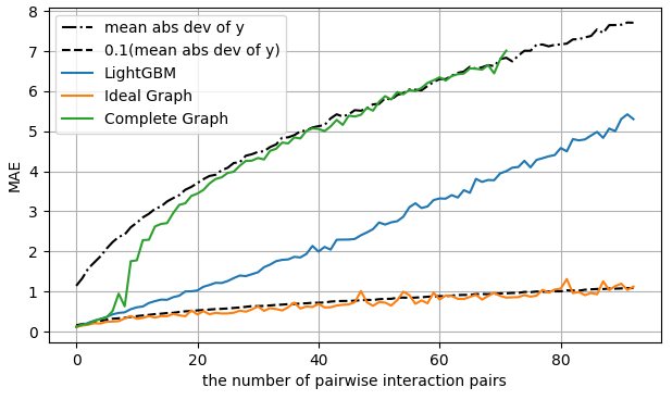
Figure 8: Predictive performance of lightGBM, GNN with complete graphs and GNN with ground truth feature graphs measured by MAE (y-axis) when the number of pairwise terms is varied (x-axis)

Figure 8 presents the results tested in synthetic datasets with 2 linear terms, that is, $y=x_{1}x_{2}+\cdots+x_{2p-1}x_{2p}+x_{2p+1}+x_{2p+2}$. The results for complete graphs and the ground truth graphs are represented by the red and blue lines, respectively. In addition, we depict the theoretical standard deviation of the datasets with a black dot line. The thick black line indicates the noise term $\epsilon$ added to the training label, which is $y+0.1\sigma$.

It is evident that greater noise, resulting from an increase in the number of features, leads to poorer prediction performance. When our GNN model is trained on complete feature graphs, it outperforms lightGBM when there are only a few pairwise terms (up to 10 in both datasets). Beyond this point, it dramatically increases, and the GNN model performs less effectively than lightGBM.

Notably, the red line plot in the right figure terminates at 40 pairwise terms (95 features or 4465 edges). The dataset in the right figure experiences memory leakage during the construction of complete feature graphs and computational processes of the model. This is why it is essential to avoid training the entire dataset using complete feature graphs when dealing with a larger number of features.

On the other hand, considering the performance of the GNN model trained on the ground truth feature graphs, the results show the lowest error compared to complete graphs and lightGBM. This underscores the value of pruning the edges of feature graphs when training models for prediction. Complete graphs not only lead to memory leaks but also capture uninformative hidden data. In conclusion, pairwise feature interaction is a beneficial property that should be retained in feature graphs to enhance the predictive performance of tabular data using GNNs.

VII-F Discussion

All results we show in this section mainly support the argument about the necessity of interaction edges in the case of a bilinear (pairwise interaction by multiplication) interaction. Moreover, it also reveals that the non-interaction edges tend to behave like noise edges to capture non-underlying information in the given dataset when feature graphs contain all interaction edges. So, if possible, we need to prune out such uninformative edges that avoid capturing noise in the dataset. However, in some cases, we may not know explicit interaction pairs to be able to keep the correct edges. Our result shows that the adjacency between interacting nodes can be weakened to only reachability via non-interaction edges in the limited number of hops by increasing the number of layers of message passing in the GNN models.

However, the results shown in this section are from only one simulated dataset. Even though the results seem obviously to infer the conclusions, we need some theoretical results to guarantee the consistency of the results in any dataset that we are focusing on. The results from Sections VII-B and VII-C motivate us to reformulate the problem into a theoretical perspective which is discussed in the next section.

VIII Case Study: Click-through-rate Prediction

We observed that it is ideal to include all known interaction edges in feature graphs. Non-interaction edges can be considered noise, capturing irrelevant information. When all interaction edges cannot be preserved, adjacency constraints can be relaxed to focus on reachability or connectedness, aided by more message passing layers. In this section, we move from simulated data to the real world problems. One of the real world problems that interactions between features are often concerned is the click-through rate (CTR) problem as a recommendation system in various application.

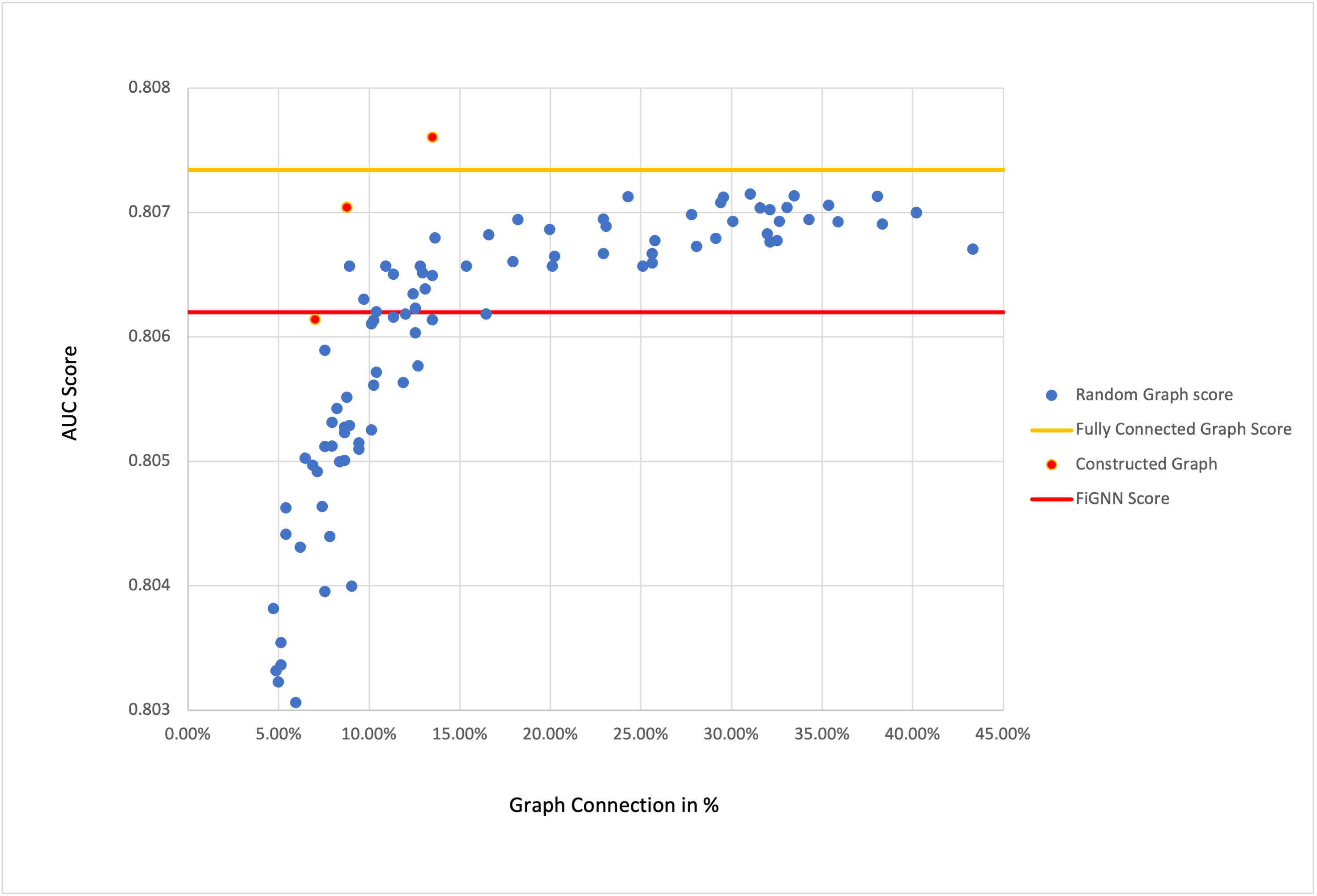
Figure 9: Comparison of AUC scores for different graph structures on the Criteo dataset. Randomly constructed sparse graphs (blue) exhibit varying performance based on connection percentage, with an optimal score of 0.8072 at 24% connectivity. The manually constructed sparse graph (orange) outperforms both the fully connected graph (yellow) and FiGNN (red) with an AUC of 0.8076 at just 13% connectivity.

In this experiment, we utilized the Criteo dataset [25] to evaluate the performance of different graph structures using the AUC score as the primary metric.

FiGNN, a widely recognized graph model for CTR prediction, achieves an AUC score of 0.8062. Initially, we generated random sparse graphs with varying percentages of connections and evaluated their performance using a simple GNN model. The optimal AUC score for randomly constructed graphs was approximately 0.8072, achieved with 24% graph connections. Subsequently, we experimented with a fully connected graph, utilizing 100% of the graph connections. The AUC score for the fully connected graph was 0.8073. Additionally, we manually constructed a sparse graph inspired by the GDCN heatmap [26]. This manually constructed graph achieved an AUC score of 0.8076 with only 13 % of the connections.

The findings of this experiment demonstrate that a simple GNN model with a randomly constructed sparse graph can outperform the FiGNN model and achieve results comparable to a fully connected graph. Moreover, the manually constructed sparse graph, designed with deliberate and meaningful connections, outperforms both the fully connected graph and FiGNN in performance. This supports the results found in our simulation.

IX Conclusion and Future Work

In this study, we investigated how the structure of feature graphs relates to their capacity to represent pairwise feature interactions within GNNs. We offered both theoretical and empirical insights on the development of sparse feature graphs. Our findings reveal that interaction edges are crucial, whereas non-interaction edges can introduce noise, which hinders the learning process of GNN models. From a theoretical standpoint, employing the Minimum Description Length (MDL) principle, we showed that feature graphs that retain only essential interaction edges provide a more efficient and interpretable representation compared to complete graphs. Empirical tests on synthetic datasets underscored the significance of interaction edges for improved prediction performance, while non-interaction edges were found to introduce noise that reduces model accuracy. Additionally, we discovered that the connection between interacting nodes, even without direct interaction edges, can enhance learning via multi-hop message passing in GNNs.

Our findings emphasize the significance of feature graph sparsity for both computational efficiency and prediction accuracy, particularly in large-scale datasets where complete graphs become useless. Furthermore, we validated the idea of our insights through a case study on click-through rate prediction, further highlighting the practical value of constructing well-designed feature graphs for real-world tasks.

For future work, our aim is to extend this study by:

1. Investigating algorithm for constructing optimal feature graphs from raw datasets, especially when prior knowledge about feature interactions is unknown.

2. Exploring feature interactions beyond pairwise relationships, such as higher-order interactions, and their implications for feature graph design.

3. Integrating dynamic graph construction methods to adapt feature graphs during model training for each instance, allowing better handling of evolving datasets and relationships.

4. Design new message-passing mechanisms specifically tailored for interaction modeling, enabling GNNs to better capture interaction patterns and relationships in feature graphs.

By addressing these directions, we hope to further advance the understanding and utility of feature graphs in GNN-based models, contributing to improved model performance and interpretability across a broad range of applications.

Proof of the Correspondence Question

To prove Theorem 3, we need some prerequisites as follows:

Proposition 9.

Let $C_{1}$ and $C_{2}$ be cluster graphs in $\mathcal{G}(n)$ for $n\in\mathbb{N}$. Then $[C_{1}]_{\sim}=[C_{2}]_{\sim}$ if and only if $C_{1}=C_{2}$.

Proof.

The backward direction is trivial. We need to prove only the forward direction. Assume that $[C_{1}]_{\sim}=[C_{2}]_{\sim}$. That is, $C_{1}\sim C_{2}$. To prove that $C_{1}=C_{2}$, we prove $E(C_{1})=E(C_{2})$, and by symmetry, we prove only $E(C_{1})\subseteq E(C_{2})$.

To prove that $E(C_{1})\subseteq E(C_{2})$, let $\{u,v\}\in E(C_{1})$ for nodes $u,v\in N_{n}$. Then $u$ and $v$ are trivially reachable in $C_{1}$. Since $C_{1}\sim C_{2}$, they also are reachable in $C_{2}$. Since $C_{2}$ is a cluster graphs, $\{u,v\}\in E(C_{2})$. Hence $E(C_{1})\subseteq E(C_{2})$, and also $E(C_{1})=E(C_{2})$. Therefore, $C_{1}=C_{2}$. ∎

Lemma 10.

The set of partitions of the set $N_{n}$, named $P(n)$, one-to-one corresponds to $\mathfrak{G}(n)$

Proof.

Observe the function $F:P(n)\to\mathfrak{G}(n)$ defined by $F(\mathfrak{A})=\left[C(\mathfrak{A})\right]_{\sim}$ for any $\mathfrak{A}\in P(n)$.

First we show that $F$ is well-defined. Let $\mathfrak{A}_{1}$ and $\mathfrak{A}_{2}$ be two partition of $N_{n}$ such that $\mathfrak{A}_{1}=\mathfrak{A}_{2}$. Since $\mathfrak{A}_{1}=\mathfrak{A}_{2}$, we have $C(\mathfrak{A}_{1})=C(\mathfrak{A}_{2})$. Then $F(\mathfrak{A}_{1})=[C(\mathfrak{A}_{1})]_{\sim}=[C(\mathfrak{A}_{2})]_{\sim}=F(\mathfrak{A}_{2}).$ Hence $F$ is well-defined.

Next, we prove injection. Let $\mathfrak{A}_{1}$ and $\mathfrak{A}_{2}$ be two partitions of $N_{n}$ such that $\mathfrak{A}_{1}\neq\mathfrak{A}_{2}$. Then, without loss of generality, there must be $A\subseteq N_{n}$ such that $A\in\mathfrak{A}_{1}$ but $A\notin\mathfrak{A}_{2}$.

Case 1: $|A|=1$. Let say $A=\{a\}$. Since $\{a\}\in\mathfrak{A}_{1}$ which is a partition, we obtain that $a\notin e$ for all edge $e\in C(\mathfrak{A}_{1})$. Since $\{a\}\notin\mathfrak{A}_{2}$, there must be some $k\in N_{n}$ such that $a,k\in Y$ for some $Y\in\mathfrak{A}_{2}$. Then $\{a,k\}\in C(\mathfrak{A}_{2})$. Hence $C(\mathfrak{A}_{1})\neq C(\mathfrak{A}_{2})$ in this case.

Case 2: Since $A\notin\mathfrak{A}_{2}$ and $|A|>1$, there are two possible sub-cases as follows:

1. There is $a\in N_{n}\setminus A$ such that $A\cup\{a\}\subseteq B$ for some partition $B\in\mathfrak{A}_{2}$.

2. There are $a,b\in A$ such that $a\neq b$ and they are in different partition in $\mathfrak{A}_{2}$.

Case 2.1: there is $a\in N_{n}\setminus A$ such that $A\cup\{a\}\subseteq B$ for some partition $B\in\mathfrak{A}_{2}$. Let $x,y\in A$. Then $\{x,a\}\notin C(\mathfrak{A}_{1})$ but $\{x,a\}\in C(\mathfrak{A}_{2})$. Hence $C(\mathfrak{A}_{1})\neq C(\mathfrak{A}_{2})$ in this case.

Case 2.2: there are $a,b\in A$ such that $a\neq b$ and they are in different partition in $\mathfrak{A}_{2}$. Then $\{a,b\}\in C(\mathfrak{A}_{1})$ but $\{a,b\}\notin C(\mathfrak{A}_{2})$. Hence $C(\mathfrak{A}_{1})\neq C(\mathfrak{A}_{2})$ in this case.

Therefore, by Proposition 9, we can conclude that $F(\mathfrak{A}_{1})\neq F(\mathfrak{A}_{2})$, and hence $F$ is injective.

Lastly, surjectivity of $F$ is trivial by considering the partition $\mathfrak{A}$ of sets which is constructed by any cluster graph $C$ and is defined as: For any nodes $u,v\in N_{n}$, they are in the same set in $\mathfrak{A}$ if $\{u,v\}\in E(C)$, and if a node $u\in N_{n}$ is isolated, then $\{u\}\in\mathfrak{A}$. Then $F(\mathfrak{A})=[C]_{\sim}$. Therefore $F$ is one-to-one correspondence between $P(n)$ and $\mathfrak{G}(n)$. Now, we are done for the correspondence question. ∎

Lemma 11.

$\mathcal{DM}(n)$ one-to-one corresponds to $P(n)$.

Proof of Lemma 11.

Observe the function $f:\mathcal{DM}\to P(n)$ defined by $f\left(\sum_{i=1}^{n}\prod_{j=1}^{m_{i}}x_{i_{j}}\right)=\left\{\left\{x_{i_{j}}\right\}_{j=1}^{m_{i}}\right\}_{i=1}^{n}$. It is obvious that $f$ is well-defined and surjective.

To prove injectivity, we proceed the proof by induction on $n$. For $n=1$, suppose that $f\left(\prod_{j=1}^{m}x_{j}\right)=f\left(\prod_{j=1}^{m^{\prime}}y_{j}\right)$. Then $\left\{\left\{x_{j}\right\}_{j=1}^{m}\right\}=\left\{\left\{y_{j}\right\}_{j=1}^{m^{\prime}}\right\}$. Since they are singleton sets, we have that $\left\{x_{j}\right\}_{j=1}^{m}=\left\{y_{j}\right\}_{j=1}^{m^{\prime}}$. Then $m=m^{\prime}$, and also $\prod_{j=1}^{m}x_{j}=\prod\left\{x_{j}\right\}_{j=1}^{m}=\prod\left\{y_{j}\right\}_{j=1}^{m^{\prime}}=\prod_{j=1}^{m^{\prime}}y_{j}$. Next, for $n>1$, we assume the induction hypothesis which is stated as $\sum_{i=1}^{k}\prod_{j=1}^{m_{i}}x_{i_{j}}=\sum_{i=1}^{k}\prod_{j=1}^{m_{i}}y_{i_{j}}$ provided $f(\sum_{i=1}^{k}\prod_{j=1}^{m_{i}}x_{i_{j}})=f(\sum_{i=1}^{k}\prod_{j=1}^{m_{i}}y_{i_{j}})$ for all $k\leq n-1$. Suppose that $f(\sum_{i=1}^{n}\prod_{j=1}^{m_{i}}x_{i_{j}})=f(\sum_{i=1}^{n}\prod_{j=1}^{m_{i}}y_{i_{j}})$. Then $\left\{\left\{x_{i_{j}}\right\}_{j=1}^{m_{i}}\right\}_{i=1}^{n}=\left\{\left\{y_{i_{j}}\right\}_{j=1}^{m_{i}}\right\}_{i=1}^{n}$. Thus $\{x_{n_{j}}\}_{j=1}^{m_{n}}\in\left\{\left\{y_{i_{j}}\right\}_{j=1}^{m_{i}}\right\}_{i=1}^{n}$. Without loss of generality, let say that $\{x_{n_{j}}\}_{j=1}^{m_{n}}=\{y_{n_{j}}\}_{j=1}^{m_{n}}$. Thus $\prod_{j=1}^{m_{n}}x_{n_{j}}=\prod_{j=1}^{m_{n}}y_{i_{j}}$ and also $\left\{\left\{x_{i_{j}}\right\}_{j=1}^{m_{i}}\right\}_{i=1}^{n-1}=\left\{\left\{y_{i_{j}}\right\}_{j=1}^{m_{i}}\right\}_{i=1}^{n-1}$. By induction hypothesis, we have $\sum_{i=1}^{n-1}\prod_{j=1}^{m_{i}}x_{i_{j}}=\sum_{i=1}^{n-1}\prod_{j=1}^{m_{i}}y_{i_{j}}$. Thus $\sum_{i=1}^{n}\prod_{j=1}^{m_{i}}x_{i_{j}}=\sum_{i=1}^{n-1}\prod_{j=1}^{m_{i}}x_{i_{j}}+\prod_{j=1}^{m_{n}}x_{n_{j}}=\sum_{i=1}^{n-1}\prod_{j=1}^{m_{i}}y_{i_{j}}+\prod_{j=1}^{m_{n}}y_{n_{j}}=\sum_{i=1}^{n}\prod_{j=1}^{m_{i}}y_{i_{j}}$. Hence $f$ is injective. Therefore, $f$ is one-to-one correspondence between $\mathcal{DM}$ and $P(n)$. ∎

Finally, from Lemma 10 and Lemma 11, Theorem 3 is obviously obtained: the set of all DMIE expession of $n$ features one-to-one corresponds to the set of feature graph up to connected component, as we needed.

Proof of the MDL for Feature Graphs

Proof of Lemma 4

Proof.

For this proof, unless indicate otherwise, we denote by $\deg(\cdot)$ the degree of node with respect to the graph $G*$. Let us denote $\hat{c}_{i}$ and $\hat{c}_{ij}$ parameters to be learned by a function $f_{G*}$. As well, we let $\hat{d}_{i}$ and $\hat{d}_{ij}$ for that of $f_{G^{*}\setminus\{i,j\}}$. Note first that $f_{G*}$ contains the term $\hat{c}_{ab}x_{a}x_{b}$, but $f_{G^{*}\setminus\{i,j\}}$ does not. Similarly, $f_{G^{*}\setminus\{i,j\}}$ contains the terms $\hat{d}_{a}x_{a}$ and $\hat{d}_{b}x_{b}$.

It is obvious that $\sum_{i=1}^{n}\mathcal{L}_{\mathbb{R}}(y_{i}-f_{G^{*}}(x_{i}))\leq\sum_{i=1}^{n}\mathcal{L}_{\mathbb{R}}(\epsilon_{i})\leq\sum_{i=1}^{n}\mathcal{L}_{\mathbb{R}}(\epsilon^{*})=n\mathcal{L}_{\mathbb{R}}(\epsilon^{*}).$ Now we claim that $\sum_{i=1}^{n}\mathcal{L}_{\mathbb{R}}(y_{i}-f_{G^{*}\setminus\{a,b\}}(x_{i}))\geq n\mathcal{L}_{\mathbb{R}}(\epsilon^{*})$. We observe that $\sum_{i=1}^{n}\mathcal{L}_{\mathbb{R}}\left(\left|y_{i}-f_{G^{*}\setminus\{a,b\}}(x_{i})\right|\right)=\sum_{i=1}^{n}\mathcal{L}_{\mathbb{R}}\left(\left|\sum_{\deg(i)=0}(c_{i}-\hat{d}_{i})x_{i}+\sum_{\{i,j\}\in E(G^{*})\setminus ab}(c_{ij}-\hat{d}_{ij})x_{i}x_{j}+\epsilon_{i}+c_{ab}x_{a}x_{b}-\hat{d}_{a}x_{a}-\hat{d}_{b}x_{b}\right|\right)=\sum_{i=1}^{n}\mathcal{L}_{\mathbb{R}}\left(\left|c_{ab}x_{a}x_{b}-\hat{d}_{a}x_{a}-\hat{d}_{b}x_{b}+\epsilon_{i}\right|\right)\geq\sum_{i=1}^{n}\mathcal{L}_{\mathbb{R}}\left(\left|\epsilon_{i}\right|\right)\geq n\mathcal{L}_{\mathbb{R}}(\epsilon^{*})$

as we desired. Therefore, $\sum_{i=1}^{n}\mathcal{L}_{\mathbb{R}}\left(y_{i}-f_{G^{*}\setminus\{a,b\}}(x_{i})\right)\geq n\mathcal{L}_{\mathbb{R}}(\epsilon^{*})\geq\sum_{i=1}^{n}\mathcal{L}_{\mathbb{R}}(y_{i}-f_{G^{*}}(x_{i})).$ By similar argument, for $\{a,b\}\notin E(G^{*})$, we obtain that $\sum_{i=1}^{n}\mathcal{L}_{\mathbb{R}}\left(\left|y_{i}-f_{G^{*}\cup\{a,b\}}(x_{i})\right|\right)=\sum_{i=1}^{n}\mathcal{L}_{\mathbb{R}}\left(\left|c_{a}x_{a}+c_{b}x_{b}-\hat{d}_{ab}x_{a}x_{b}+\epsilon_{i}\right|\right)\geq n\mathcal{L}_{\mathbb{R}}(\epsilon^{*})$ Therefore, $\sum_{i=1}^{n}\mathcal{L}_{\mathbb{R}}\left(y_{i}-f_{G^{*}\cup\{a,b\}}(x_{i})\right)\geq n\mathcal{L}_{\mathbb{R}}(\epsilon^{*})\geq\sum_{i=1}^{n}\mathcal{L}_{\mathbb{R}}(y_{i}-f_{G^{*}}(x_{i})).$ ∎

Proof of Proposition 5

Proof.

For the removing interaction edge, by our initial assumptions, we have $\sum_{\deg(i)=0}\mathcal{L}_{\mathbb{R}}(\hat{c}_{i})\approx\sum_{\deg(i)=0}\mathcal{L}_{\mathbb{R}}(\hat{d}_{i})$ and $\sum_{\{i,j\}\in E(G*)}\mathcal{L}_{\mathbb{R}}(\hat{c}_{ij})\approx\mathcal{L}_{\mathbb{R}}(\hat{c}_{ab})+\sum_{\{i,j\}\in E(G*)\setminus\{\{a,b\}\}}\mathcal{L}_{\mathbb{R}}(\hat{d}_{ij}).$ It is obvious that the term $\sum_{i=1}^{n}\mathcal{L}_{\mathbb{R}}(x_{i})$ does not depend on representation. Then we have $\mathcal{L}(S_{G^{*}},f_{G^{*}\setminus\{a,b\}})-\mathcal{L}(S_{G^{*}},f_{G^{*}})=\mathcal{L}_{\mathbb{R}}(|E(G*)|-1)-\mathcal{L}_{\mathbb{R}}(|E(G*)|)+\mathcal{L}_{\mathbb{R}}(\hat{d}_{a})+\mathcal{L}_{\mathbb{R}}(\hat{d}_{b})-\mathcal{L}_{\mathbb{R}}(\hat{c}_{ab})+\sum_{i=1}^{n}\mathcal{L}_{\mathbb{R}}(y_{i}-f_{G^{*}\setminus\{a,b\}}(x_{i}))-\sum_{i=1}^{n}\mathcal{L}_{\mathbb{R}}(y_{i}-f_{G^{*}}(x_{i}))\geq\mathcal{L}_{\mathbb{R}}(\hat{d}_{a})+\mathcal{L}_{\mathbb{R}}(\hat{d}_{b})-\mathcal{L}_{\mathbb{R}}(\hat{c}_{ab})-D\geq 0$, by what we assume above and Lemma 4.

Next, we prove the argument about adding a non-interaction edge $\{a,b\}\notin E(G^{*})$. Similarly, we have that $\mathcal{L}(S_{G^{*}},f_{G^{*}\cup\{a,b\}})-\mathcal{L}(S_{G^{*}},f_{G^{*}})=\mathcal{L}_{\mathbb{R}}(|E(G*)|+1)-\mathcal{L}_{\mathbb{R}}(|E(G*)|)+\mathcal{L}_{\mathbb{R}}(\hat{d}_{ab})-\mathcal{L}_{\mathbb{R}}(\hat{c}_{a})-\mathcal{L}_{\mathbb{R}}(\hat{c}_{b})+\sum_{i=1}^{n}\mathcal{L}_{\mathbb{R}}(y_{i}-f_{G^{*}\cap\{a,b\}}(x_{i}))-\sum_{i=1}^{n}\mathcal{L}_{\mathbb{R}}(y_{i}-f_{G^{*}}(x_{i}))\geq D+\mathcal{L}_{\mathbb{R}}(\hat{d}_{ab})-\mathcal{L}_{\mathbb{R}}(\hat{c}_{a})-\mathcal{L}_{\mathbb{R}}(\hat{c}_{b})\geq 0$ ∎

References

- [1] Z. Li, Z. Cui, S. Wu, X. Zhang, and L. Wang, “Fi-gnn: Modeling feature interactions via graph neural networks for ctr prediction,” Proceedings of the 28th ACM International Conference on Information and Knowledge Management, 2019.
- [2] J. Lee, I. Lee, and J. Kang, “Self-attention graph pooling,” ArXiv, vol. abs/1904.08082, 2019.
- [3] V. Nannen, “A short introduction to model selection, kolmogorov complexity and minimum description length (mdl),” ArXiv, vol. abs/1005.2364, 2010.
- [4] J. Rissanen, “Modeling by shortest data description*,” Autom., vol. 14, pp. 465–471, 1978.
- [5] P. D. Grünwald, “The minimum description length principle (adaptive computation and machine learning),” 2007.
- [6] J. H. Friedman and B. E. Popescu, “Predictive learning via rule ensembles,” The Annals of Applied Statistics, vol. 2, pp. 916–954, 2008.
- [7] S. Rendle, “Factorization machines,” 2010 IEEE International Conference on Data Mining, pp. 995–1000, 2010.
- [8] Y.-C. Juan, Y. Zhuang, W.-S. Chin, and C.-J. Lin, “Field-aware factorization machines for ctr prediction,” Proceedings of the 10th ACM Conference on Recommender Systems, 2016.
- [9] J. Xiao, H. Ye, X. He, H. Zhang, F. Wu, and T.-S. Chua, “Attentional factorization machines: Learning the weight of feature interactions via attention networks,” ArXiv, vol. abs/1708.04617, 2017.
- [10] F. Zhou, H. Zhou, Z. Yang, and L. Yang, “Emd2fnn: A strategy combining empirical mode decomposition and factorization machine based neural network for stock market trend prediction,” Expert Syst. Appl., vol. 115, pp. 136–151, 2019.
- [11] H. Guo, R. Tang, Y. Ye, Z. Li, and X. He, “Deepfm: A factorization-machine based neural network for ctr prediction,” ArXiv, vol. abs/1703.04247, 2017.
- [12] D. Bahdanau, K. Cho, and Y. Bengio, “Neural machine translation by jointly learning to align and translate,” CoRR, vol. abs/1409.0473, 2014.
- [13] A. Sarkar, D. Das, V. Sembium, and P. M. Comar, “Dual attentional higher order factorization machines,” Proceedings of the 16th ACM Conference on Recommender Systems, 2022.
- [14] W. Cheng, Y. Shen, and L. Huang, “Adaptive factorization network: Learning adaptive-order feature interactions,” ArXiv, vol. abs/1909.03276, 2019.
- [15] K. Wang, C.-Y. Shen, and W. Ma, “Adnfm: An attentive densenet based factorization machine for ctr prediction,” 2020.
- [16] P. Wen, W. Yuan, Q. Qin, S. Sang, and Z. Zhang, “Neural attention model for recommendation based on factorization machines,” Applied Intelligence, vol. 51, pp. 1829 – 1844, 2020.
- [17] Z. Li, S. Wu, Z. Cui, and X. Zhang, “Graphfm: Graph factorization machines for feature interaction modeling,” ArXiv, vol. abs/2105.11866, 2021.
- [18] F. Feng, X. He, H. Zhang, and T.-S. Chua, “Cross-gcn: Enhancing graph convolutional network with $k$k-order feature interactions,” IEEE Transactions on Knowledge and Data Engineering, vol. 35, pp. 225–236, 2020.
- [19] Z. Li, S. Wu, Z. Cui, and X. Zhang, “Graphfm: Graph factorization machines for feature interaction modeling,” ArXiv, vol. abs/2105.11866, 2021.
- [20] A. Chang, Q. Wang, and X. Zhang, “Neural matrix factorization model based on latent factor learning,” 2023 3rd International Conference on Neural Networks, Information and Communication Engineering (NNICE), pp. 52–56, 2023.
- [21] K. Zhou, Z. Liu, R. Chen, L. Li, S.-H. Choi, and X. Hu, “Table2graph: Transforming tabular data to unified weighted graph,” in International Joint Conference on Artificial Intelligence, 2022.
- [22] T. Kipf and M. Welling, “Semi-supervised classification with graph convolutional networks,” ArXiv, vol. abs/1609.02907, 2016.
- [23] Y. Rong, W. Huang, T. Xu, and J. Huang, “Dropedge: Towards deep graph convolutional networks on node classification,” in International Conference on Learning Representations, 2019.
- [24] Y. Shi, Z. Huang, W. Wang, H. Zhong, S. Feng, and Y. Sun, “Masked label prediction: Unified massage passing model for semi-supervised classification,” ArXiv, vol. abs/2009.03509, 2020.
- [25] C. Labs, “Criteo display advertising challenge dataset,” https://www.kaggle.com/c/criteo-display-ad-challenge/data, 2014.
- [26] F. Wang, H. Gu, D. Li, T. Lu, P. Zhang, and N. Gu, “Towards deeper, lighter and interpretable cross network for ctr prediction,” Proceedings of the 32nd ACM International Conference on Information and Knowledge Management, 2023.