Interleaved Gibbs Diffusion for Constrained Generation

Abstract

We introduce Interleaved Gibbs Diffusion (IGD), a novel generative modeling framework for mixed continuous-discrete data, focusing on constrained generation problems. Prior works on discrete and continuous-discrete diffusion models assume factorized denoising distribution for fast generation, which can hinder the modeling of strong dependencies between random variables encountered in constrained generation. IGD moves beyond this by interleaving continuous and discrete denoising algorithms via a discrete time Gibbs sampling type Markov chain. IGD provides flexibility in the choice of denoisers, allows conditional generation via state-space doubling and inference time scaling via the ReDeNoise method. Empirical evaluations on three challenging tasks—solving 3-SAT, generating molecule structures, and generating layouts—demonstrate state-of-the-art performance. Notably, IGD achieves a 7% improvement on 3-SAT out of the box and achieves state-of-the-art results in molecule generation without relying on equivariant diffusion or domain-specific architectures. We explore a wide range of modeling, and interleaving strategies along with hyperparameters in each of these problems.

1 Introduction

Autoregressive models have been highly successful at modeling languages in a token by token fashion. While finetuned autoregressive (AR) models can produce realistic texts and maintain lengthy human-like conversations, they are known to fail at simple planning and reasoning tasks. One hypothesis is that AR generation is not suited for generating tokens where non-trivial constraints have to be satisfied. There have been efforts such as Chain-of-Thought prompting (Wei et al., 2022) and O1 (OpenAI, 2024) which force the model to “think over” the solution in many steps before answering.

Diffusion models, another class of generative models, start with pure noise and slowly denoise to obtain a sample from the desired distribution (Ho et al., 2020; Song et al., 2020). While its outstanding applications have been in the context of generating images (i.e, continuous data) (Saharia et al., 2022; Rombach et al., 2022), it has been successfully extended to discrete data (Austin et al., 2021; Lou et al., 2023). This model has shown promising results in planning and constrained generation in a wide range of tasks, such as layout generation, molecule generation, 3SAT, SuDoKu (Ye et al., 2024) and traveling salesman problem (Zhang et al., 2024), outperforming AR models. This is attributed to diffusion models being able to parse the entire set of generated tokens multiple times during denoising.

Algorithms based on D3PM (Austin et al., 2021) as presented in prior works (Inoue et al., 2023; Ye et al., 2024) and mixed mode diffusion based works such as (Hua et al., 2024) assume that the denoising process samples from a product distribution of the tokens, which seems unreasonable in cases of constrained generation where the tokens can be highly dependent. It would be desirable if partial denoising of a token (continuous or discrete) is dependent on current denoised status of all other tokens. Alternative proposals such as Concrete Score Matching (Meng et al., 2022), SEDD (Lou et al., 2023), symmetric diffusion ((Zhang et al., 2024)) and Glauber Generative Model (GGM) (Varma et al., 2024) do not assume such a factorization. Symmetric diffusion considers the special case of generating permutations using riffle shuffle as the noising process and derives algorithms for denoising it exactly. This demonstrates gains in a variety of planning problems. GGM is a discrete diffusion model which denoises a lazy random walk exactly by learning to solve a class of binary classification problems.

Gibbs Sampler is a Markov chain which samples jointly distributed random variables by resampling one co-ordinate at a time from the accurate conditional distribution. This has been studied widely in Theoretical Computer Science, Statistical Physics, Bayesian Inference and Probability Theory (Geman & Geman, 1984; Turchin, 1971; Gelfand & Smith, 1990; Martinelli, 1999; Levin & Peres, 2017). While the original form gives a Markov Chain Monte Carlo (MCMC) algorithm, (Varma et al., 2024) considered a learned, time dependent, systematic scan variant of the Gibbs sampler for generative modeling over discrete spaces.

In this work, we extend the principle of time dependent Gibbs sampler to mixed mode data - sequences with both discrete tokens and continuous vectors. Such problems arise naturally in applications like Layout Generation (Levi et al., 2023) and Molecule Generation (Hua et al., 2024).

Our Contributions:

We introduce an effective method to train a diffusion based model to solve planning problems and constrained generation problems where the sequence being generated could involve both discrete and continuous tokens. The key contributions include:

1. The Interleaved Gibbs Diffusion (IGD) framework for sampling from mixed distributions (mix of continuous and discrete variables), by performing Gibbs sampling type denoising, one element at a time. This does not assume factorizability of the denoising process.

2. Theoretical justification for the proposed denoising process and a novel adaptation of Tweedie’s formula to the IGD setting where we require learn conditional score function by estimating the the cumulative noise over multiple round robins despite the conditioning chain during the process.

3. A framework for conditional sampling when some elements are fixed via state space doubling inspired by DLT (Levi et al., 2023) and an inference time algorithm called ReDeNoise inspired by SDEdit (Meng et al., 2021). ReDeNoise can potentially boost the accuracy of generation at the cost of additional compute.

4. State-of-the-art performance in constrained generation problems such as 3-SAT, molecule generation and layout generation. In molecule generation and layout generation, we outperform existing discrete-continuous frameworks and achieve SoTA results without relying on specialized diffusion processes or domain-specific architectures. In 3-SAT, we outperform the SoTA diffusion model out of the box and study how accuracy improves with the model size and dataset size.

Organization: Preliminaries are given in Section 2. The IGD framework, with continuous and discrete denoisers as black boxes, is described in Section 3. The inference time scaling ReDeNoise algorithm is given in Section 3.3 and the conditional sampling algorithm is given in Section 3.4. Multiple recipes to design and train the black box denoisers are given in Section 4. Experimental results are presented in Section 6, Conclusion and Future Work in Section 7.

2 Preliminaries

Notation

Let $\mathcal{X}$ be a finite set, let $L$ be the sequence length such that $L=L_{1}+L_{2}$, $L_{1},L_{2}\in\mathbb{N}\cup\{0\}$. Let $d_{L_{1}+1},\dots,d_{L}\in\mathbb{N}$ be the continuous dimensions. We let our state space to be $\mathcal{S}_{L}=\mathcal{X}^{L_{1}}\times_{i=L_{1}+1}^{L}\mathbb{R}^{d_{i}}$. The elements of this set can be represented as a tuple/sequence of length $L$. For any $s\in\mathcal{S}_{L}$, let $s_{i}$ denote the element in $s$ at position $i$ in the tuple. Note that, $s_{i}$ is a discrete token from the set $\mathcal{X}$ if $i\leq L_{1}$ and it is a continuous vector sampled from $\mathbb{R}^{d_{i}}$ if $L_{1}<i\leq L$. Let $s_{-i}$ denote the tuple of length $L-1$ obtained by removing the element at the $i^{\text{th}}$ position of $s$.

Problem Setup

Given samples $s_{1},\dots,s_{N}$ from the target distribution $\pi$ over $\mathcal{S}_{L}$, the task is to learn a model which can generate more samples approximately from $\pi$. We will call $\mathcal{D}=\{s_{1},\dots,s_{N}\}$ to be the dataset.

3 Interleaved Gibbs Diffusion

We now describe the Interleaved Gibbs Diffusion (IGD) framework for sampling from a target distribtuion $\pi$ over $\mathcal{S}_{L}$, given access to discrete and continuous denoisers which satisfy certain properties. We first describe the forward noising process and then the reverse denoising process using the given denoisers. In IGD, both the forward noising and reverse denoising processes operate one element at a time. Our noising process is illustrated in Figure 1.

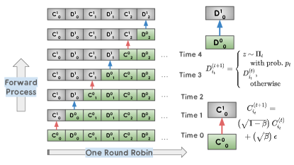
Figure 1: Interleaved Noising Process: Sequential noising of discrete tokens ($D_{s}$) and continuous vectors ($C_{s}$). Noising occurs one element at a time, keeping other elements unchanged.

3.1 Forward Noising Process

The forward noising process takes a sample $s$ from the target distribution $\pi$ and applies a discrete time Markov chain to obtain the trajectory $s^{(0)},s^{(1)},\dots,s^{(T)}$, where $T$ is the total number of timesteps. We refer to $t$ as the sequence time. Note that $s^{(0)}=s$. For each $t$, we choose a position $i_{t}\in\{1,2,\dots,L\}$ to be noised at sequence time $t$. In this work, we choose $i_{t}$ in a round-robin fashion from some permutation of $\{1,2,\dots,L\}$ so that all positions are noised exactly once after every $L$ sequence timesteps; we call this permutation the interleaving pattern. Given $i_{t}$, the corresponding sequence element $s_{i_{t}}$ can either be discrete or continuous, based on which we either perform either discrete noising or continuous noising.

Discrete Noising

If $s_{i_{t}}$ is discrete (i.e, $i_{t}\leq L_{1}$), following (Varma et al., 2024), we consider token $\phi\notin\mathcal{X}$ and define a probability distribution $\Pi_{t}$ over $\mathcal{X}\cup\{\phi\}$. Note that $\Pi_{t}$ depends on the sequence time $t$. We refer to $\Pi_{t}$ as the discrete noise schedule. Then the discrete noising process is as follows:

Sample $z_{t}\sim\Pi_{t}$ independent of $s^{(t)}$. Then we have:

$$s^{(t+1)}_{j}=\begin{cases}z_{t},&\text{if }j=i_{t}\text{ and }z_{t}\neq\phi\\ s^{(t)}_{j},&\text{otherwise }\end{cases}$$

Continuous Noising

If $s_{i_{t}}$ is continuous (i.e, $L_{1}<i_{t}\leq L_{2}$), we use $m_{i_{t}}^{t}$ to denote the number of times position $i_{t}$ has been visited by sequence time $t$ (including the visit at $t$). Let $m=\max_{i_{t}}m_{i_{t}}^{T}$. Define $[\tilde{\beta}_{j}]_{j=1}^{m}$ to be a monotonically increasing sequence, which we refer to as the continuous noise schedule. Then, the continuous noising process is given by: $s^{(t+1)}_{i_{t}}=\left(\sqrt{1-\tilde{\beta}_{m_{i_{t}}^{t}}}\right)s^{(t)}_{i_{t}}+\left(\sqrt{\tilde{\beta}_{m_{i_{t}}^{t}}}\right)\epsilon^{(t)}$ where $\epsilon^{(t)}\sim\mathcal{N}(0,\mathbf{I})$. Note that $s^{(t+1)}_{j}=s^{(t)}_{j}\quad\forall j\neq i_{t}$.

Lemma 3.1 (Mild extension of Lemma $1$ in (Varma et al., 2024)).

Denote the distribution of $s^{(t)}$ by $P_{t}$. Suppose $\Pi_{t}\left(\cdot|\mathcal{X}\right)=\Pi\left(\cdot|\mathcal{X}\right)$ for all $t$, $\Pi_{t}(\phi)\leq 1-\epsilon$ for some $\epsilon>0$ and $\lim_{T\rightarrow\infty}\sum_{j}\log\left(1-\tilde{\beta}_{j}\right)=-\infty$. As $T\rightarrow\infty$, $P_{T}$ converges to the product distribution: $\Pi\left(\cdot|\mathcal{X}\right)^{L_{1}}\times_{i=L_{1}+1}^{L}\mathcal{N}\left(0,\mathbf{I}_{d_{i}}\right)$ .

Co-ordinate wise independent noising:

The noising process of any element $s_{i_{t}}^{(t)}$ at any time $t$ is independent of other elements; this allows us to sample $s^{(t)}$ at any time $t$ directly from $s^{(0)}$ without having to compute $s^{(1)},s^{(2)},...,s^{(t)}$ sequentially (Algorithm given in Appendix C).

3.2 Reverse Denoising Process

The reverse denoising process takes a sample $\hat{s}^{(T)}$ from $P_{T}$ as the input and applies a discrete time Markov chain to obtain the trajectory $\hat{s}^{(T)},\hat{s}^{(T-1)},\dots,\hat{s}^{(0)}$, where $T$ is the total number of sequence timesteps. Recall that $i_{t}$ denotes the position which was noised at time $t$ during the forward process.

Given $\hat{s}^{(t+1)}$, we set $\hat{s}^{(t)}_{-i_{t}}=\hat{s}^{(t+1)}_{-i_{t}}$. Depending on whether $\hat{s}^{(t+1)}_{i_{t}}$ is discrete (resp. continuous) we use the discrete denoiser (resp. continuous denoiser) to sample $\hat{s}^{(t)}_{i_{t}}$ (${s}^{(t+1)}$ is the sample from the forward process at time $t+1$):

Discrete Denoiser is a (learned) sampling algorithm which can sample from $\hat{P}_{t,i_{t}}(\cdot|s)$, a probability distribution over $\mathcal{X}$ given $s$ as the input. $\hat{P}_{t,i_{t}}(\cdot|s=\hat{s}^{(t+1)})$ approximates one of the following:

$\mathbb{P}(s^{(t)}_{i_{t}}=\cdot|s^{(t+1)}_{-i_{t}}=\hat{s}^{(t+1)}_{-i_{t}})$ or $\mathbb{P}(s^{(t)}_{i_{t}}=\cdot|s^{(t+1)}=\hat{s}^{(t+1)})$

Discrete Denoising Step: $\texttt{DiscDen}(\hat{s}^{(t)},i_{t},t)$ outputs a sample $\hat{s}^{(t)}_{i_{t}}\sim\hat{P}_{t,i_{t}}\left(\cdot|s=\hat{s}^{(t+1)}\right)$.

Continuous Denoiser is a (learned) sampling algorithm which can sample from the distribution $\hat{P}_{t,i_{t}}(\cdot|s)$ over $\mathbb{R}^{d_{i_{t}}}$ given $\hat{s}^{(t+1)}$ as the input. $\hat{P}_{t,i_{t}}(\cdot|s=\hat{s}^{(t+1)})$ approximates the conditional distribution $\mathbb{P}(s^{(t)}_{i_{t}}=\cdot|s^{(t+1)}=\hat{s}^{(t+1)})$.

Continuous Denoising Step: $\texttt{ContDen}(\hat{s}^{(t)}_{i_{t}},i_{t},t)$ outputs a sample $\hat{s}^{(t)}_{i_{t}}\sim\hat{P}_{t,i_{t}}\left(\cdot|s=\hat{s}^{(t+1)}\right)$.

Lemma 3.2.

Assume $\hat{s}^{(T)}\sim P_{T}$ and assume we have access to ideal discrete and continuous denoisers. Then, $\hat{s}^{(0)}$ obtained after $T$ steps of reverse denoising process, will be such that $\hat{s}^{(0)}\sim\pi$.

From the definition of the discrete and continuous denoisers, it is clear that unlike the forward process, the reverse process is not factorizable. However, by sacrificing factorizability, we are able to achieve exact reversal of the forward process, provided we have access to ideal denoisers. The denoising algorithm is detailed in Algorithm 1.

0:  $\hat{s}^{T}\sim P_{T}$, discrete denoiser DiscDen , continuous denoiser ContDen, noise positions $\{i_{t}\}$

0: $\hat{s}^{0}\sim{\pi}$

 for $t\in[T,T-1,\dots,1]$ do

  $\hat{s}^{(t-1)}_{-i_{t}}=\hat{s}^{(t)}_{-i_{t}}$

  if $\hat{s}^{(t)}_{i_{t}}$ is discrete then

   $\hat{s}^{(t-1)}_{i_{t}}=\texttt{DiscDen}(\hat{s}^{(t)},i_{t},t)$

  else

   $\hat{s}^{(t-1)}_{i_{t}}=\texttt{ContDen}(\hat{s}^{(t)},i_{t},t)$

  end if

 end for

Algorithm 1 Interleaved Gibbs Diffusion: Ideal Denoising

3.3 ReDeNoise Algorithm

Inspired by (Meng et al., 2021), we now propose a simple but effective mechanism for quality improvements at inference time. Given a sample obtained through complete reverse process $\hat{s}^{(0)}$, we now repeat the following two steps $N_{R}$ times: (1) Noise $\hat{s}^{(0)}$ for $T_{R}$ rounds to obtain $\hat{s}^{(T_{R})}$. (2) Denoise $\hat{s}^{(T_{R})}$ back to $\hat{s}^{(0)}$. While $N_{R}$ decides the number of times the noise-denoise process is repeated, $T_{R}$ decides how much noising is done each time. These are hyperparameters which can be tuned to suit the task at hand.

3.4 Conditional Generation

We train the model for conditional generation - i.e, generate a subset of the co-ordinates conditioned on the rest. We adopt the state-space doubling strategy, inspired by (Levi et al., 2023). A binary mask vector is created indicating whether each element in the sequence is part of the conditioning or not; for vectors in $\mathbb{R}^{d}$, a mask is created for each element in the vector. The mask is now embedded/projected and added to the discrete/continuous embedding and fed into the model while training. Further, during the forward and reverse processes, the conditioned elements are not noised/denoised.

4 Training the Denoisers

Having established the IGD framework, we now describe strategies to train the discrete and continuous denoisers, which have been black boxes in our discussion so far.

4.1 Training the Discrete Denoiser

Throughout this subsection, we use $g_{\theta}$ to denote a parameterised neural network which is trained to be the discrete denoiser. $g_{\theta}$ takes input from the space $\mathcal{S}_{L}\times\{0,1,\dots,T-1\}$ and outputs logits in the space $[0,1]^{\absolutevalue{\mathcal{X}}}$. We now describe two strategies to train $g_{\theta}$:

4.1.1 $\absolutevalue{\mathcal{X}}$-ary classification

In this approach, the objective is to learn $\mathbb{P}\left({s}^{(t)}_{i_{t}}=\cdot|{s}^{(t+1)}=\hat{s}^{(t)}\right)$. So, we directly train the model to predict ${s}^{(t)}_{i_{t}}$ given ${s}^{(t+1)}$. Since there are $\absolutevalue{\mathcal{X}}$ discrete tokens in the vocabulary, this is a $\absolutevalue{\mathcal{X}}$-ary classification problem, where the input is ${s}^{(t+1)}$ and the corresponding label is ${s}^{(t)}_{i_{t}}$. Hence, we minimize the cross-entropy loss: $\mathcal{L}_{CE}\left(\theta;{s}^{(t+1)},t\right)=-\log\left(g_{\theta}^{s_{i_{t}}}\left({s}^{(t+1)},t\right)\right)$ where $g^{s_{i_{t}}}_{\theta}(\cdot)$ denotes the logit corresponding to token ${s}^{(t)}_{i_{t}}$.

4.1.2 Binary classification

In this approach, the objective is to learn $\mathbb{P}\left({s}^{(t)}_{i_{t}}=\cdot|{s}^{(t+1)}_{-i_{t}}=\hat{s}^{(t)}_{-i_{t}}\right)$. We adapt Lemma 3.1 from (Varma et al., 2024) to simplify this objective:

Lemma 4.1.

Let $s\in\mathcal{S}^{L}$. Then, for $x\in\mathcal{X}$ and discrete ${s}^{(t)}_{i_{t}}$, we can write $\mathbb{P}\left({s}^{(t)}_{i_{t}}=x|{s}^{(t+1)}_{-i_{t}}={s}_{-i_{t}}\right)$ as :

$$\frac{\mathbb{P}(z_{t}=x)}{\mathbb{P}(z_{t}=\phi)}\left(\frac{1}{\mathbb{P}\left({z_{t}}=x|{s}^{(t+1)}_{-i_{t}}={s}_{-i_{t}},{s}^{(t+1)}_{i_{t}}=x\right)}-1\right)$$

where $\left(s^{(0)},\dots s^{(T)},\right)$ is obtained from forward process.

Hence, it is sufficient for the model to learn $\mathbb{P}\left({z_{t}}=x|{s}^{(t+1)}_{-i_{t}}={s}_{-i_{t}},{s}^{(t+1)}_{i_{t}}=x\right)$ for all $x\in\mathcal{X}$. This can be formulated as a binary classification task: Given ${s}^{(t+1)}_{-i_{t}}$ and ${s}^{(t+1)}_{i_{t}}=x$ as the input, predict whether $z_{t}=x$ or $z_{t}=\phi$. Hence, we minimize the binary cross-entropy loss: $\mathcal{L}_{BCE}\left(\theta;{s}^{(t+1)}_{-i_{t}},t\right)=-\mathbf{1}_{z_{t}\neq\phi}\log\left(g_{\theta}^{x}\left({s}^{(t+1)}_{-i_{t}},t\right)\right)-\mathbf{1}_{z_{t}=\phi}\log\left(1-g_{\theta}^{x}\left({s}^{(t+1)}_{-i_{t}},t\right)\right)$ where $g^{x}_{\theta}(\cdot)$ denotes the logit corresponding to token $x$.

Preliminary experiments (Appendix F.4) gave better results with the binary classification loss; hence we use binary classification for training the discrete denoiser.

4.2 Training the Continuous Denoiser

In continuous diffusion, the noising (and denoising) process follows an SDE; the entire process happens in an uninterrupted fashion. However, in IGD, the noising and denoising happen with interruptions, because of the sequential nature. Thus, in the reverse process, the conditioning surrounding a continuous element changes every time it is picked for denoising. By an adaptation of the standard Tweedie’s formula and exploiting the fact that forward noising process for every element is independent of other elements, we show that using the current conditioning and estimating the cumulative noise added from the beginning (across interruptions) still reverses the continuous elements in an interleaved manner. This is the novelty behind Lemma 4.2.

Suppose we are given a sample $s^{(t)}$ from the distribution at time $t$. Let $\stackrel{{\scriptstyle d}}{{=}}$ denote equality in distribution. Suppose $x_{0}=s_{i_{t}}^{(t)}\in\mathbb{R}^{d_{i_{t}}}$ and consider the Orstein-Uhlenbeck Process $dx_{\tau}=-x_{\tau}d\tau+\sqrt{2}dB_{\tau}$ with standard Brownian motion $B_{\tau}$. Then $x_{\tau_{0}}|s^{(t)}\stackrel{{\scriptstyle d}}{{=}}s_{i_{t}}^{(t+1)}|s^{(t)}$ whenever $\tau_{0}=\frac{1}{2}\log(\tfrac{1}{1-\beta_{m_{i_{t}}^{t}}})$. Based on the observations in (Song et al., 2020; Ho et al., 2020), the reverse SDE given by

$$x_{\tau}^{\mathsf{rev}}=x_{\tau}^{\mathsf{rev}}d\tau+2\nabla\log q_{\tau_{0}-\tau}(x^{\mathsf{rev}}_{\tau}|s_{-i_{t}}^{(t)})\tau+\sqrt{2}dB_{\tau}$$ (1)

is such that if $x^{\mathsf{rev}}_{0}=s_{i_{t}}^{(t+1)}$ then $x^{\mathsf{rev}}_{\tau_{0}}|s^{(t+1)}\stackrel{{\scriptstyle d}}{{=}}s_{i_{t}}^{(t)}|s^{(t+1)}$ where $q_{\tau}(\cdot|s^{(t+1)})$ is the conditional density function of $x_{\tau}$. We use DDPM (Ho et al., 2020) to sample from $\mathbb{P}(s_{i_{t}}^{(t)}=\cdot|s^{(t+1)})$ by learning the score function $\nabla\log q_{\tau}(\cdot|s_{-i_{t}}^{(t+1)})$ and then discretizing the reverse SDE in Equation (1).

To obtain a more precise discretization, we divide the noising at sequence timestep $t$ into $K_{i_{t}}^{t}$ element timesteps (whenever $s_{i_{t}}$ is a continuous vector). We define $s_{i_{t}}^{(t,0)}=s_{i_{t}}^{(t)}$, $s_{i_{t}}^{(t,K_{i_{t}}^{t})}=s_{i_{t}}^{(t+1)}$, and for $k\in[0,1,\dots,K_{i_{t}}^{t}-1]$:

$$s^{(t,k+1)}_{i_{t}}\sim\mathcal{N}\left(\left(\sqrt{1-{\beta}(t,k)}\right)s^{(t,k)}_{i_{t}},\left({{\beta}(t,k)}\right)\mathbf{I}\right)$$

where ${\beta}$ is a continuous noise schedule which outputs a scalar given $(t,k)$ as input. Following the popular DDPM (Ho et al., 2020) framework, we rewrite the noising process as:

$$s^{(t,k+1)}_{i_{t}}=\left(\sqrt{\bar{\alpha}(t,k)}\right)s^{(0)}_{i_{t}}+\left(\sqrt{1-\bar{\alpha}(t,k)}\right)\epsilon$$ (2)

where $\epsilon\sim\mathcal{N}(0,\mathbf{I})$ and $\bar{\alpha}$ is a cumulative noise schedule obtained from $\hat{\beta}$. The exact relations between $\tilde{\beta}$ (defined in 3.1), ${\beta}$ and $\bar{\alpha}$ are given in Appendix B. With this discretization, the reverse process becomes:

$$\hat{s}^{(t,k)}_{i_{t}}=\frac{\left(\hat{s}^{(t,k+1)}_{i_{t}}-{\beta}(t,k+1)p({s}^{(t,k+1)})\right)}{\sqrt{1-{\beta}(t,k+1)}}+\sqrt{{\beta}(t,k+1)}\epsilon^{\prime}$$

where $\epsilon^{\prime}\in\mathcal{N}(0,\mathbf{I})$ and $p({s}^{(t,k+1)})$ is the score function $\nabla_{{s}_{i_{t}}^{(t,k+1)}}\log q({s}_{i_{t}}^{(t,k+1)}|{s}_{-i_{t}}^{(t,k+1)})$. Now to learn the score function, we use the following Lemma:

Lemma 4.2.

Under the considered forward process where noising occurs independently, we have:

$$\nabla_{{s}_{i_{t}}^{(t,k+1)}}\log q({s}_{i_{t}}^{(t,k+1)}|{s}_{-i_{t}}^{(t,k+1)})=-\frac{1}{\sqrt{1-\bar{\alpha}}}\mathbb{E}\left[\epsilon|{s}^{(t,k+1)}\right]$$

Hence, if we can learn $\mathbb{E}\left[\epsilon|{s}^{(t,k+1)}\right]$ exactly, the forward process can be reversed exactly assuming you start from the stationary distribution. Hence, we minimize the regression loss: $\norm{\epsilon-g\left({s}^{(t,k+1)},t,k\right)}_{2}^{2}$ where $g(\cdot)$ is a neural network which is trained to predict $\epsilon$ given $\left(\hat{s}^{(t,k+1)},t,k\right)$.

Apart from DDPM sampling, we also evaluated DDIM, which is an ODE based method. However, preliminary results (reported in Appendix G.3) indicated that DDPM performs better. A detailed description of the exact training and inference algorithms we use is given in Appendix D.

5 Model Architecture

Inspired by (Peebles & Xie, 2023), we use a transformer-based architecture closely resembling Diffusion Transformers (DiTs) for the model. Since DiT has been designed for handling discrete tokens, we modify the architecture slightly to accommodate continuous vectors as well. However, we keep modifications to a minimum, so that the proposed architecture can still benefit from DiT design principles. Our proposed architecture, which we refer to as Discrete-Continuous (Dis-Co) DiT, is illustrated in Figure 2.

Figure 2(a) gives a high-level overview of the model with $N$ Dis-Co DiT blocks stacked on top of each other. Discrete embeddings, continuous projections and their corresponding time embeddings are passed into the Dis-Co DiT blocks. Figure 2(b) details the structure of a single Dis-Co DiT block. The discrete embeddings and continuous vectors are processed as in a regular transformer block; however the discrete and continuous time information ($(t,k)$ variables) is incorporated using adaptive layer normalization (Xu et al., 2019). Exact details are given in Appendix E.

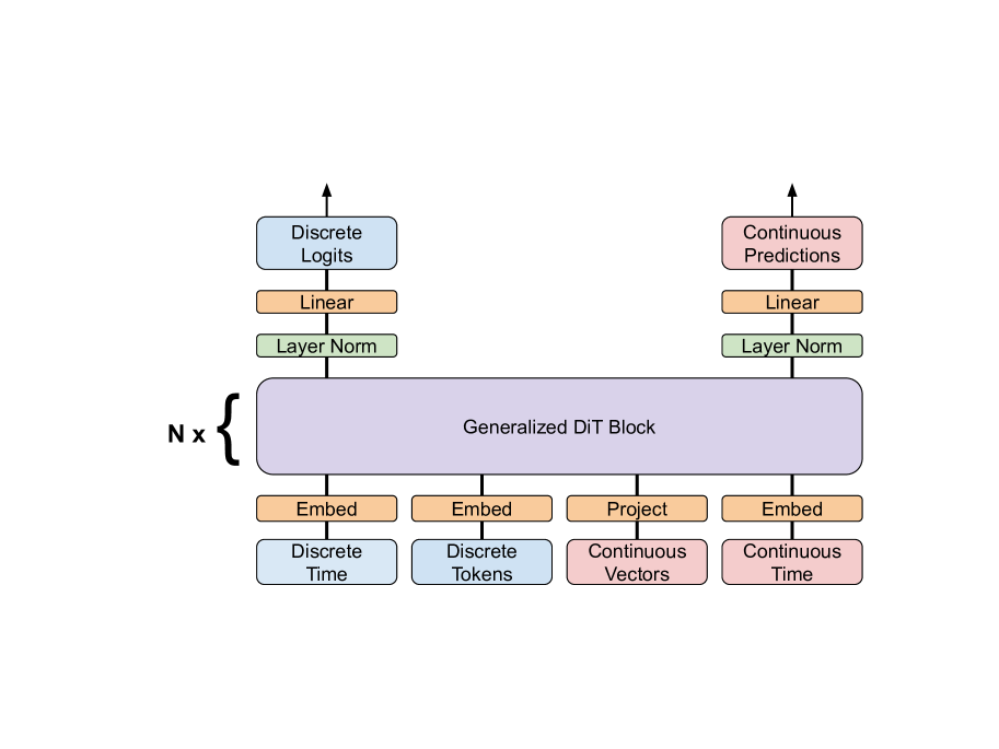
(a)

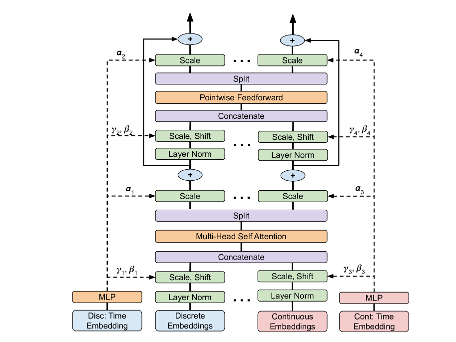
(b)

Figure 2: Dis-Co DiT Architecture: (a) illustrates overall architecture, with both discrete and continuous inputs and outputs (b) shows detailed architecture of a single block, where time information is incorporated through adaptive layer normalization.

6 Experiments

We evaluate the IGD framework on three different tasks: Layout Generation, Molecule Generation and the Boolean Satisfiability problem. While the first two tasks involve generating both discrete tokens and continuous vectors, 3SAT involves only discrete tokens. Nevertheless, all three problems are constrained generation problems and can hence benefit from the exact reversal of IGD framework.

6.1 Layout Generation

6.1.1 Background

Layout generation aims to generate coherent arrangements of UI elements (e.g., buttons, text blocks) or document components (e.g., titles, figures, tables) that satisfy both functional requirements and aesthetic principles. This problem is important in various applications of graphic design and interface prototyping.

Formally, each layout is a set of $N$ elements $\{e_{i}\}_{i=1}^{N}$. Each element $e_{i}$ is represented by a discrete category $t_{i}\in\mathbb{N}$ and a continuous bounding box vector $\mathbf{p}_{i}\in\mathbb{R}^{4}$. We use the parameterization $\mathbf{p}_{i}=[x_{i},\,y_{i},\,l_{i},\,w_{i}]^{\top}$, where $(x_{i},\,y_{i})$ represents the upper-left corner of the bounding box, and $(l_{i},\,w_{i})$ its length and width, respectively.

6.1.2 Experimental Setup

We adopt a setup similar to (Guerreiro et al., 2025) for standardized comparison to existing layout generation methods.

Datasets:

We evaluate our method on two popular layout generation datasets:
1. PubLayNet (Zhong et al., 2019): Contains layouts of scientific documents annotated with 5 element categories.
2. RICO (Deka et al., 2017): Provides user-interface (UI) layouts with 25 element categories.
Following prior works (Jiang et al., 2023; Zhang et al., 2023), layouts containing more than 20 elements are discarded from the datasets.

Evaluation metrics:

Following previous works (Inoue et al., 2023; Chen et al., 2024), we evaluate our method primarily using two metrics described below:

1. Frechet Inception Distance (FID) (Heusel et al., 2017): This metric measures the distance between the generated and real data distributions by comparing the features extracted from a neural network. For FID calculation, we use the feature space from the same network with identical weights as in (Zhang et al., 2023).

2. Maximum Intersection over Union (mIoU) (Kikuchi et al., 2021): This calculates the maximum IoU between bounding boxes of the generated layouts and real data layouts with the same element category.

Results on additional evaluation metrics (Alignment and Overlap) are presented in Appendix F.1. Baseline metrics in Table 1 are reported as given in (Guerreiro et al., 2025).

Tasks: Results are presented on three common layout generation tasks:

1. Unconditional Generation: No constraints.

2. Category-Conditioned Generation: Element categories are specified.

3. Category + Size-Conditioned Generation: Both element categories and sizes are specified.

Baselines:

We compare with state-of-the-art methods: Diffusion-based approaches include: LayoutDM (Inoue et al., 2023), which applies discrete diffusion to handle element categories and positions; LayoutDiffusion (Zhang et al., 2023), employing iterative refinement with tailored noise schedules for layout attributes; and DLT (Levi et al., 2023), a hybrid model separating element categories and coordinates into distinct diffusion processes. Flow-based: LayoutFlow (Guerreiro et al., 2025) leverages trajectory learning for efficient sampling. Non-diffusion baselines comprise: LayoutTransformer (Gupta et al., 2021) (autoregressive sequence generation), LayoutFormer++ (Jiang et al., 2023) (serializes constraints into token sequences for conditional generation), and NDN-none (Lee et al., 2020) (adversarial training without constraints).

6.1.3 Results

Table 1 presents quantitative results across different tasks and datasets. On RICO, we outperform all baselines in category-conditioned and category+size-conditioned generation, with competitive performance on unconditioned generation. On PubLayNet, we achieve the best FID in unconditioned and category+size-conditioned generation.

Notably, IGD outperforms DLT, a discrete-continuous diffusion model which assumes factorizability of the reverse process, on most of the tasks in both datasets by a significant margin. This further demonstrates the effectiveness of our framework in comparison to existing discrete-continuous diffusion models. We also note that models such as LayoutDM and LayoutDiffusion employ specialized diffusion processes tailored for layout generation, whereas we directly employ our discrete-continuous diffusion framework without further modifications. We refer to Appendix F for further implementation details, example generations as well as extensive ablations.

Table 1: Layout Generation: Quantitative results on the RICO and PubLayNet datasets. Refer to section 6.1.2 for details on evaluation tasks and metrics.

RICO
	Unconditioned			Category Conditioned			Category$+$Size Conditioned
Method	FID$\downarrow$	mIoU$\uparrow$		FID$\downarrow$	mIoU$\uparrow$		FID$\downarrow$	mIoU$\uparrow$
LayoutTransformer	24.32	0.587		-	-		-	-
LayoutFormer++	20.20	0.634		2.48	0.377		-	-
NDN-none	-	-		13.76	0.350		-	-
LayoutDM	4.43	0.582		2.39	0.341		1.76	0.424
DLT	13.02	0.566		6.64	0.326		6.27	0.424
LayoutDiffusion	2.49	0.620		1.56	0.345		-	-
LayoutFlow	2.37	0.570		1.48	0.322		1.03	0.470
Ours	2.54	0.594		1.06	0.385		0.96	0.524

PubLayNet
	Unconditioned			Category Conditioned			Category$+$Size Conditioned
Method	FID$\downarrow$	mIoU$\uparrow$		FID$\downarrow$	mIoU$\uparrow$		FID$\downarrow$	mIoU$\uparrow$
LayoutTransformer	30.05	0.359		-	-		-	-
LayoutFormer++	47.08	0.401		10.15	0.333		-	-
NDN-none	-	-		35.67	0.310		-	-
LayoutDM	36.85	0.382		39.12	0.348		29.91	0.436
DLT	12.70	0.431		7.09	0.349		5.35	0.426
LayoutDiffusion	8.63	0.417		3.73	0.343		-	-
LayoutFlow	8.87	0.424		3.66	0.350		1.26	0.454
Ours	8.32	0.419		4.08	0.402		0.886	0.553

6.2 Molecule Generation

6.2.1 Background

Molecule generation aims to synthesize new valid molecular structures from a distribution learned through samples. Recently, generative models trained on large datasets of valid molecules have gained traction. In particular, diffusion-based methods have shown strong capabilities in generating discrete atomic types and their corresponding 3D positions.

We represent a molecule with $n$ atoms by $(z_{i},\mathbf{p}_{i})_{i=1}^{n}$, where $z_{i}\in\mathbb{N}$ is the atom’s atomic number and $\mathbf{p}_{i}\in\mathbb{R}^{3}$ is the position. We focus on organic molecules with covalent bonding, where bond orders (single, double, triple, or no bond) between atoms are assigned using a distance-based lookup table following (Hoogeboom et al., 2022).

6.2.2 Experimental Setup

We closely follow the methodology used in prior works (Hua et al., 2024) and (Hoogeboom et al., 2022) for 3D molecule generation. Further details are given below:

Datasets:

We evaluate on the popular QM9 benchmark (Ramakrishnan et al., 2014) which contains organic molecules with up to 29 atoms and their 3D coordinates. We adopt the standardized 100K/18K/13K train/val/test split to ensure fair comparison with prior works. We generate all atoms, including hydrogen, since this is a harder task.

Evaluation metrics:

We adopt four metrics following prior works (Hua et al., 2024) and (Hoogeboom et al., 2022):

1. Atom Stability: The fraction of atoms that satisfy their valency. Bond orders (single, double, triple, no bond) are determined from pairwise atomic distances using a distance-based lookup table given in (Hoogeboom et al., 2022).

2. Molecule Stability: Fraction of molecules where all atoms are stable.

3. Validity: RDKit-based (Landrum et al., 2006) molecular sanitization checks, as in (Hoogeboom et al., 2022). These checks include: chemical plausibility of bond angles and lengths, absence of disconnected components, kekulization of aromatic rings, and more.

4. Uniqueness: Fraction of unique and valid molecules.

Baselines:

We compare with state-of-the-art methods: E-NF (equivariant normalizing flows) (Köhler et al., 2020) models molecular generation via invertible flow transformations. G-SchNet (Gebauer et al., 2019) employs an autoregressive architecture with rotational invariance. Diffusion-based approaches include EDM (Hoogeboom et al., 2022) (with SE(3)-equivariant network (Fuchs et al., 2020)) , GDM (Hoogeboom et al., 2022) (non-equivariant variant of EDM), and DiGress (Vignac et al., 2023a) (discrete diffusion for atoms/bonds without 3D geometry). GeoLDM (Xu et al., 2023) leverages an equivariant latent diffusion process, while MUDiff (Hua et al., 2024) unifies discrete (atoms/bonds) and continuous (positions) diffusion with specialized attention blocks. While (Peng et al., 2023) and (Vignac et al., 2023b) are also diffusion based methods, they are not directly comparable due to reasons we list in G.1.

6.2.3 Results

Table 2 compares our method with others on QM9. Notably, without relying on specialized equivariant diffusion or domain-specific architectures, IGD attains strong performance across four key metrics. Our model achieves 98.9% atom stability and 95.4% molecular validity, equaling or surpassing other methods. Our model achieves a molecule stability of 90.5%, surpassing the baselines. While not the best in ‘uniqueness’, our approach still yields more than 95% unique samples among the valid molecules. In addition, we observe noticeably lower standard deviations than most baselines, reflecting consistent performance.

Notably, applying ReDeNoise at inference yielded an improvement of 4.99% in molecular stability. Further implementation details, and ablation studies examining design choices such as the interleaving pattern, discrete and continuous noise schedules are presented in Appendix G.

Table 2: Molecule Generation: Quantitative results on QM9 benchmark. We report mean (standard deviation) across 3 runs, each with 10K generated samples. Refer to section 6.2.2 for details on evaluation metrics.

Method	Atom stable (%)	Mol stable (%)	Validity (%)	Uniqueness (%)
E-NF	85.0	4.9	40.2	39.4
G-Schnet	95.7	68.1	85.5	80.3
GDM	97.6	71.6	90.4	89.5
EDM	${98.7}\pm{0.1}$	82.0$\pm{0.4}$	91.9 $\pm 0.5$	90.7 $\pm 0.6$
DiGress	${98.1}\pm{0.3}$	79.8$\pm{5.6}$	95.4 $\pm 1.1$	97.6 $\pm 0.4$
GeoLDM	98.9$\pm{0.1}$	89.4$\pm{0.5}$	93.8 $\pm 0.4$	92.7 $\pm 0.5$
MUDiff	${98.8}\pm{0.2}$	89.9$\pm{1.1}$	95.3 $\pm 1.5$	99.1 $\pm 0.5$
Ours	98.9$\pm{0.03}$	90.5 $\pm 0.15$	95.4 $\pm 0.2$	95.6 $\pm 0.1$
Data	99.0	95.2	99.3	100.0

6.3 Boolean Satisfiability Problem

6.3.1 Background

The Boolean Satisfiability (SAT) problem is the task of determining whether there exists a binary assignment to the variables of a given Boolean expression (in Conjunctive Normal Form (CNF)) that makes it evaluate to True. SAT is a canonical NP-Complete problem (Cook, 1971) and underlies a broad range of real-world applications in formal hardware/software verification, resource scheduling, and other constraint satisfaction tasks (Clarke et al., 2001; Gomes et al., 2008; Vizel et al., 2015).

Our goal is to find a valid assignment for the Boolean variables, when the given CNF formula is satisfiable. Let $n$ be the number of variables and $m$ the number of clauses. In Random $k$-SAT, a well-studied variation of SAT, the relative difficulty of an instance is determined by the clause density $\frac{m}{n}$. There is a sharp transition between satisfiable and unsatisfiable instances of random 3-SAT at the critical clause density $\alpha_{\mathrm{sat}}(k=3)$, when m is set close to $m=4.258n+58.26n^{-\frac{2}{3}}$ (Ding et al., 2015). Following the setup of (Ye et al., 2024), we choose $m$ close to this threshold to focus on relatively hard random 3-SAT instances.

6.3.2 Experimental Setup

Datasets: We consider two experimental setups:

Setup 1 (Single $n$): We follow the train and test partitions from (Ye et al., 2024), which provide separate datasets for $n\!=5,7,$ and $9$, for direct comparison. Specifically, $n=5$ and $n=7$, use a training set of 50K samples each, while for $n=9$, the training set consists of 100K samples.

Setup 2 (Combined $n$): We then move to a more challenging, large-scale setting by extending the range of $n$ up to 20. Following the same generation procedure, for each $n$ in ${6,7,\dots,20}$, we generate 1M training samples, resulting in a combined dataset of 15M instances. In this setup, we train a single model on the aggregated data covering all $n$ from 6 to 20. Figure 3 illustrates how the model’s accuracy varies with $n$ under different model sizes.

More details on data generation and model configuration are provided in Appendix H.

Baselines: We compare against two types of baseline models: 1) Autoregressive Models with a GPT-2 architecture (Radford et al., 2019) trained from scratch and 2) Discrete diffusion models in (Ye et al., 2024) (MDM) that applies adaptive sequence- and token-level reweighting to emphasize difficult subgoals in planning and reasoning. MDM has demonstrated strong performance on tasks such as Sudoku and Boolean Satisfiability compared to standard autoregressive and discrete diffusion approaches.

Table 3: SAT: Accuracy with increasing number of variables $n$. Separate model trained for each $n$

Method	Params	$n=5$	$n=7$	$n=9$
GPT-2 Scratch	6M	97.6	85.6	73.3
MDM	6M	100.0	95.9	87.0
Ours	6M	100.0	98.0	94.5
	85M	-	99.9	99.9

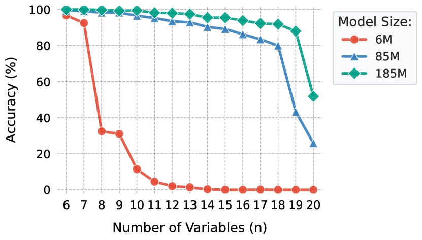
Figure 3: SAT: Accuracy for different number of variables across model sizes trained on a combined dataset for n in $6,7\dots,20$.

6.3.3 Results

In Table 3, we see that our method consistently outperforms the autoregressive (GPT-2) and diffusion-based (MDM) baselines across different choices for $n$. This performance gap is more pronounced for larger $n$: at $n=9$, our model achieves 94.5% accuracy, compared to 87.0% for MDM and 73.3% for GPT-2. Scaling the model to 85M parameters further reaches near-perfect accuracy (99.9%) for $n=7$ and $n=9$, thus highlighting the crucial role of model capacity in handling complex SAT instances.

For Setup 2, Figure 3 reveals a steep accuracy drop for the 6M-parameter model; it starts declining around $n=8$ and approaches zero by $n=12$. In contrast, the 85M-parameter model remains robust up to $n=18$, and an even larger 185M-parameter model sustains high accuracy near $n=19$. This degradation trend aligns with the theoretical hardness of random 3-SAT, where solution spaces become exponentially sparse as $n$ increases. Larger models postpone this accuracy drop underscoring a direct relationship between parameter count and combinatorial reasoning capacity.

7 Conclusion and Future Work

We propose IGD, a diffusion framework for mixed-mode data sampling. We theoretically establish the exactness of this framework and empirically validate its effectiveness across multiple tasks through extensive experiments. Future work can explore other choices for samplers such as Flow Matching/Rectified Flow. In layout generation and molecule generation, specialized architectures and losses could be incorporated to further improve performance.

Impact Statement

This paper contributes to the advancement of machine learning by introducing a novel constrained sampling algorithm. While generative machine learning models, particularly in text and image generation, have raised societal concerns, our work focuses on molecule generation, layout generation, and 3-SAT, using publicly available datasets. At this stage, we foresee no direct societal impact. However, we acknowledge that future applications of our method in sensitive domains may necessitate a more thorough evaluation of potential societal implications.

Appendix A Proofs

A.1 Lemma 3.1

Statement:

Denote the distribution of $s^{(t)}$ by $P_{t}$. Suppose $\Pi_{t}\left(\cdot|\mathcal{X}\right)=\Pi\left(\cdot|\mathcal{X}\right)$ for all $t$, $\Pi_{t}(\phi)\leq 1-\epsilon$ for some $\epsilon>0$ and $\lim_{T\rightarrow\infty}\sum_{j}\log\left(1-\tilde{\beta}_{j}\right)=-\infty$. As $T\rightarrow\infty$, $P_{T}$ converges to the product distribution: $\Pi\left(\cdot|\mathcal{X}\right)^{L_{1}}\times_{i=L_{1}+1}^{L}\mathcal{N}\left(0,\mathbf{I}_{d_{i}}\right)$ .

Proof:

We closely follow the proof of Lemma 1 in (Varma et al., 2024).

Note that the forward noising for each element is independent of all other elements. Hence, it suffices to consider the noising of each element separately.

Consider a discrete element. By assumption, the probability of not choosing $\phi$:

$$1-\Pi(\phi)\geq\epsilon$$

where $\epsilon>0$ for all. Further, when $\phi$ is not chosen at time $t$, then the distribution of the discrete token is $\Pi(\cdot|\mathcal{X})$ for all time $\geq t$ independent of other tokens. The probability of choosing only $\phi$ until time $t$ is at most $(1-\epsilon)^{t}$ and this goes to $0$ as $t\rightarrow\infty$. Therefore with probability $1$, asymptotically, every discrete element is noised to the distribution $\Pi\left(\cdot|\mathcal{X}\right)$.

Consider a continuous vector at position $i$. From the definition of the forward process, we have:

$$s^{(t+1)}_{i}=\left(\sqrt{1-\tilde{\beta}_{m_{i}^{t}}}\right)s^{(t)}_{i}+\left(\sqrt{\tilde{\beta}_{m_{i}^{t}}}\right)\epsilon$$ (3)

where $\epsilon\sim\mathcal{N}(0,\mathbf{I})$. Merging the Gaussians, we have:

$$s^{(t+1)}_{i}=\left(\sqrt{\tilde{\alpha}_{m_{i}^{t}}}\right)s^{(0)}_{i}+\left(\sqrt{1-\tilde{\alpha}_{m_{i}^{t}}}\right)\epsilon$$

where:

$$\tilde{\alpha}_{m_{i}^{t}}=\prod_{j=0}^{m_{i}^{t}}(1-\tilde{\beta}_{j})$$

Since $m_{i}^{t}$ denotes the number of times the position $i$ is visited by sequence time $t$, $m_{i}^{t}\rightarrow\infty$ as $t\rightarrow\infty$. Hence, from the assumption $\lim_{T\rightarrow\infty}\sum_{j}\log\left(1-\tilde{\beta}_{j}\right)=-\infty$, we have $\lim_{t\rightarrow\infty}\tilde{\alpha}_{m_{i}^{t}}=0$ and hence the continuous vector will converge to an independent Gaussian with variance $1$ per continuous dimension.

A.2 Lemma 3.2

Statement:

Assume $\hat{s}^{(T)}\sim P_{T}$ and assume we have access to ideal discrete and continuous denoisers. Then, $\hat{s}^{(0)}$ obtained after $T$ steps of reverse denoising process, will be such that $\hat{s}^{(0)}\sim\pi$.

Proof:

Recall that $s^{(t)}\in\mathcal{S}_{L}$ denotes the the sequence at sequence time $t$ of the forward process. Further, $P_{t}$ denotes the probability measure of $s^{(t)}$ over $\mathcal{S}_{L}$. $\hat{s}^{(t)}\in\mathcal{S}_{L}$ denotes the the sequence at sequence time $t$ of the reverse process and let $\hat{P}_{t}$ denote the probability measure of $\hat{s}^{(t)}$ over $\mathcal{S}_{L}$.

We now prove the lemma by induction. Assume that $\hat{s}^{(t+1)}\overset{d}{=}{s}^{(t+1)}$, i.e., ${P}_{t+1}=\hat{P}_{t+1}$. Consider a measurable set $\mathcal{A}$ such that $\mathcal{A}\subseteq\mathcal{S}_{L}$ . Let $y\sim\hat{P}_{t+1}$. From the measure decomposition theorem, we have:

$$\mathbb{P}(\hat{s}^{(t)}\in\mathcal{A})=\int_{y}\mathbb{P}\left(\hat{s}^{(t)}\in\mathcal{A}|\hat{s}^{(t+1)}=y\right)d\hat{P}_{t+1}(y)$$

From the induction assumption, we can rewrite this as:

$$\mathbb{P}(\hat{s}^{(t)}\in\mathcal{A})=\int_{y}\mathbb{P}\left(\hat{s}^{(t)}\in\mathcal{A}|\hat{s}^{(t+1)}=y\right)d{P}_{t+1}(y)$$

From the definition of the reverse process, we know that $\hat{s}^{(t)}_{-i_{t}}=\hat{s}^{(t+1)}_{-i_{t}}$. Therefore, we have:

$$\mathbb{P}\left(\hat{s}^{(t)}\in\mathcal{A}|\hat{s}^{(t+1)}=y\right)=\mathbb{P}\left(\hat{s}^{(t)}_{i_{t}}\in\mathcal{A}_{-i_{t}}\left(y_{-i_{t}}\right)|\hat{s}^{(t+1)}=y\right)$$

where $\mathcal{A}_{-i_{t}}\left(y_{-i_{t}}\right)=\{x_{i_{t}}:x\in\mathcal{A},x_{-i_{t}}=y_{-i_{t}}\}$. Depending on the reverse process chosen, we have:

$$\mathbb{P}\left(\hat{s}^{(t)}_{i_{t}}\in\mathcal{A}_{-i_{t}}\left(y_{-i_{t}}\right)|\hat{s}^{(t+1)}=y\right) =\mathbb{P}\left({s}^{(t)}_{i_{t}}\in\mathcal{A}_{-i_{t}}\left(y_{-i_{t}}\right)|s^{(t+1)}=y\right)\quad\text{or}$$

$$\mathbb{P}\left(\hat{s}^{(t)}_{i_{t}}\in\mathcal{A}_{-i_{t}}\left(y_{-i_{t}}\right)|\hat{s}^{(t+1)}=y\right) =\mathbb{P}\left({s}^{(t)}_{i_{t}}\in\mathcal{A}_{-i_{t}}\left(y_{-i_{t}}\right)|s^{(t+1)}_{-i_{t}}=y_{-i_{t}}\right)$$

Case 1: $\mathbb{P}\left(\hat{s}^{(t)}_{i_{t}}\in\mathcal{A}_{-i_{t}}\left(y_{-i_{t}}\right)|\hat{s}^{(t+1)}=y\right)=\mathbb{P}\left({s}^{(t)}_{i_{t}}\in\mathcal{A}_{-i_{t}}\left(y_{-i_{t}}\right)|s^{(t+1)}=y\right)$

We have:

$$\mathbb{P}\left(\hat{s}^{(t)}\in\mathcal{A}|\hat{s}^{(t+1)}=y\right)=\mathbb{P}\left({s}^{(t)}_{i_{t}}\in\mathcal{A}_{-i_{t}}\left(y_{-i_{t}}\right)|s^{(t+1)}=y\right)$$

And hence:

$$\mathbb{P}(\hat{s}^{(t)}\in\mathcal{A}) =\int_{y}\mathbb{P}\left({s}^{(t)}_{i_{t}}\in\mathcal{A}_{-i_{t}}\left(y_{-i_{t}}\right)|s^{(t+1)}=y\right)d{P}_{t+1}(y)$$

$$=\mathbb{P}({s}^{(t)}\in\mathcal{A})$$

Case 2: $\mathbb{P}\left(\hat{s}^{(t)}_{i_{t}}\in\mathcal{A}_{-i_{t}}\left(y_{-i_{t}}\right)|\hat{s}^{(t+1)}=y\right)=\mathbb{P}\left({s}^{(t)}_{i_{t}}\in\mathcal{A}_{-i_{t}}\left(y_{-i_{t}}\right)|s^{(t+1)}_{-i_{t}}=y_{-i_{t}}\right)$

We have:

$$\mathbb{P}\left(\hat{s}^{(t)}\in\mathcal{A}|\hat{s}^{(t+1)}=y\right)=\mathbb{P}\left({s}^{(t)}_{i_{t}}\in\mathcal{A}_{-i_{t}}\left(y_{-i_{t}}\right)|s^{(t+1)}_{-i_{t}}=y_{-i_{t}}\right)$$

And hence:

$$\mathbb{P}(\hat{s}^{(t)}\in\mathcal{A}) =\int_{y}\mathbb{P}\left({s}^{(t)}_{i_{t}}\in\mathcal{A}_{-i_{t}}\left(y_{-i_{t}}\right)|s^{(t+1)}_{-i_{t}}=y_{-i_{t}}\right)d{P}_{t+1}(y)$$

By measure decomposition theorem ${P}_{t+1}(y)$ is factorizable as:

$${P}_{t+1}(y)={P}_{t+1,-i_{t}}(y_{-i_{t}}){P}_{t+1,i_{t}}(y_{i_{t}}|y_{-i_{t}})$$

Therefore:

$$\mathbb{P}(\hat{s}^{(t)}\in\mathcal{A}) =\int_{y}\mathbb{P}\left({s}^{(t)}_{i_{t}}\in\mathcal{A}_{-i_{t}}\left(y_{-i_{t}}\right)|s^{(t+1)}_{-i_{t}}=y_{-i_{t}}\right)\left(d{P}_{t+1,-i_{t}}(y_{-i_{t}})\right)\left(d{P}_{t+1,i_{t}}(y_{i_{t}}|y_{-i_{t}})\right)$$

$$=\int_{y_{-i_{t}}}\mathbb{P}\left({s}^{(t)}_{i_{t}}\in\mathcal{A}_{-i_{t}}\left(y_{-i_{t}}\right)|s^{(t+1)}_{-i_{t}}=y_{-i_{t}}\right)\left(d{P}_{t+1,i_{t}}(y_{i_{t}}|y_{-i_{t}}))\right)\int_{y_{i_{t}}}\left(d{P}_{t+1,i_{t}}(y_{i_{t}})\right)$$

$$=\mathbb{P}({s}^{(t)}\in\mathcal{A})$$

Hence, we have $\hat{s}^{(t)}\overset{d}{=}{s}^{(t)}$, i.e. ${P}_{t}=\hat{P}_{t}$. Therefore, by induction $\hat{P}_{0}=\pi$, provided $\hat{P}_{T}={P}_{T}$.

A.3 Lemma 4.2

Statement:

Under the considered forward process where noising occurs independently, we have:

$$\nabla_{{s}_{i_{t}}^{(t,k+1)}}\log q({s}_{i_{t}}^{(t,k+1)}|{s}_{-i_{t}}^{(t,k+1)})=-\frac{1}{\sqrt{1-\bar{\alpha}}}\mathbb{E}\left[\epsilon|{s}^{(t,k+1)}\right]$$

Proof:

Let us split $\hat{s}^{(t,k+1)}=\left[\hat{s}_{i_{t}}^{(t,k+1)}\;\hat{s}_{-i_{t}}^{(t,k+1)}\right]$. Note that, $\hat{s}_{i_{t}}^{(t,k+1)}$ is the continuous part that is being de noised.

$$\nabla_{\hat{s}_{i_{t}}^{(t,k+1)}}\log q(\hat{s}_{i_{t}}^{(t,k+1)}|\hat{s}_{-i_{t}}^{(t,k+1)})\hfill =\frac{\nabla_{\hat{s}_{i_{t}}^{(t,k+1)}}q(\hat{s}_{i_{t}}^{(t,k+1)}|\hat{s}_{-i_{t}}^{(t,k+1)})}{q(\hat{s}_{i_{t}}^{(t,k+1)}|\hat{s}_{-i_{t}}^{(t,k+1)})}$$

$$=\frac{\nabla_{\hat{s}_{i_{t}}^{(t,k+1)}}q(\hat{s}_{i_{t}}^{(t,k+1)}|\hat{s}_{-i_{t}}^{(t,k+1)})q(\hat{s}_{-i_{t}}^{(t,k+1)})}{q(\hat{s}_{i_{t}}^{(t,k+1)}|\hat{s}_{-i_{t}}^{(t,k+1)})q(\hat{s}_{-i_{t}}^{(t,k+1)})}$$

$$=\frac{\nabla_{\hat{s}_{i_{t}}^{(t,k+1)}}q(\hat{s}_{i_{t}}^{(t,k+1)},\hat{s}_{-i_{t}}^{(t,k+1)})}{q(\hat{s}_{i_{t}}^{(t,k+1)},\hat{s}_{-i_{t}}^{(t,k+1)})}$$

$$=\frac{\nabla_{\hat{s}_{i_{t}}^{(t,k+1)}}\int q(\hat{s}_{i_{t}}^{(t,k+1)},\hat{s}_{-i_{t}}^{(t,k+1)}|s_{i_{t}}^{(0)})q(s_{i_{t}}^{(0)})ds_{i_{t}}^{(0)}}{q(\hat{s}_{i_{t}}^{(t,k+1)},\hat{s}_{-i_{t}}^{(t,k+1)})}$$

$$\overset{(a)}{=}\frac{\nabla_{\hat{s}_{i_{t}}^{(t,k+1)}}\int q(\hat{s}_{i_{t}}^{(t,k+1)}|s_{i_{t}}^{(0)})q(\hat{s}_{-i_{t}}^{(t,k+1)}|s_{i_{t}}^{(0)})q(s_{i_{t}}^{(0)})ds_{i_{t}}^{(0)}}{q(\hat{s}_{i_{t}}^{(t,k+1)},\hat{s}_{-i_{t}}^{(t,k+1)})}$$

$$\overset{(b)}{=}\frac{\int\frac{-\epsilon}{\sqrt{1-\bar{\alpha}}}q(\hat{s}_{i_{t}}^{(t,k+1)}|s_{i_{t}}^{(0)})q(\hat{s}_{-i_{t}}^{(t,k+1)}|s_{i_{t}}^{(0)})q(s_{i_{t}}^{(0)})ds_{i_{t}}^{(0)}}{q(\hat{s}_{i_{t}}^{(t,k+1)},\hat{s}_{-i_{t}}^{(t,k+1)})}$$

$$\overset{(a)}{=}\frac{\int\frac{-\epsilon}{\sqrt{1-\bar{\alpha}}}q(\hat{s}_{i_{t}}^{(t,k+1)},\hat{s}_{-i_{t}}^{(t,k+1)},s_{i_{t}}^{(0)})ds_{i_{t}}^{(0)}}{q(\hat{s}_{i_{t}}^{(t,k+1)},\hat{s}_{-i_{t}}^{(t,k+1)})}$$

$$=\int\frac{-\epsilon}{\sqrt{1-\bar{\alpha}}}q(s_{i_{t}}^{(0)}|\hat{s}_{i_{t}}^{(t,k+1)},\hat{s}_{-i_{t}}^{(t,k+1)})ds_{i_{t}}^{(0)}$$ (4)

In the RHS of the chain in (A.3), we observe that $\hat{s}^{t,k+1}$ is being conditioned on and given $\hat{s}^{t,k+1}$, $\epsilon$ is a function only of $s_{i_{t}}^{(0)}$ from (2). Therefore, the above chain yields:

$$\nabla_{\hat{s}_{i_{t}}^{(t,k+1)}}\log q(\hat{s}_{i_{t}}^{(t,k+1)}|\hat{s}_{-i_{t}}^{(t,k+1)})=\frac{1}{\sqrt{1-\bar{\alpha}}}\mathbb{E}\left[-\epsilon|\hat{s}^{(t,k+1)}\right]$$ (5)

This is the exactly $\frac{g_{\theta}(\cdot)}{\sqrt{1-\bar{\alpha}}}$ if the estimator was a perfect MMSE estimator.

Justifications:- (a) observe that conditioned on $s_{i_{t}}^{(0)}$, how $i_{t}$-th element is noised in the forward process is independent of all other elements. This gives rise to the conditional independence.(b) We exchange the integral and the $\nabla$ operator. Let $q(x|y)$ be conditionally Gaussian, i.e. $x|y\sim\mathcal{N}(\sqrt{\bar{\alpha}}y;(1-\bar{\alpha}))$, then it is a property of the conditional Gaussian random variable that $\nabla_{x}q(x|y)=-\left(\frac{x-\sqrt{\bar{\alpha}}y}{1-\bar{\alpha}}\right)*q(x|y)$. Taking $x=\hat{s}_{i_{t}}^{t,k}$ and $y=s_{i_{t}}^{(0)}$ from (2), we see that: $\nabla_{\hat{s}_{i_{t}}^{(t,k+1)}}q(\hat{s}_{i_{t}}^{(t,k+1)}|s_{i_{t}}^{(0)})=\frac{-\epsilon}{\sqrt{1-\bar{\alpha}}}*q(\hat{s}_{i_{t}}^{(t,k+1)}|s_{i_{t}}^{(0)})$.

Appendix B Connection between $\tilde{\beta},\beta$ and $\bar{\alpha}$

From subsection 3.1, we have:

$$s^{(t+1)}_{i_{t}}=\left(\sqrt{1-\tilde{\beta}_{m_{i_{t}}^{t}}}\right)s^{(t)}_{i_{t}}+\left(\sqrt{\tilde{\beta}_{m_{i_{t}}^{t}}}\right)\epsilon^{(t)}$$ (6)

And from subsection 4.2, we have:

$$s^{(t,k+1)}_{i_{t}}=\left(\sqrt{1-{\beta}(t,k)}\right)s^{(t,k)}_{i_{t}}+\left(\sqrt{{\beta}(t,k)}\right)\epsilon$$ (7)

where $s^{(t,0)}_{i_{t}}=s^{(t)}_{i_{t}}$ and $s^{(t,K_{i_{t}}^{t})}_{i_{t}}=s^{(t+1)}_{i_{t}}$. Define ${\alpha}(t,k)=1-{\beta}(t,k)$. Then, we have:

$$s^{(t,k+1)}_{i_{t}}=\left(\sqrt{\prod_{k^{\prime}=0}^{k}{\alpha}(t,k^{\prime})}\right)s^{(t,0)}_{i_{t}}+\left(\sqrt{1-{\prod_{k^{\prime}=0}^{k}{\alpha}(t,k^{\prime})}}\right)\epsilon$$

where we have merged the Gaussians. Setting $k=K_{i_{t}}^{t}-1$ and comparing (6) and (7), we have:

$$\tilde{\beta}_{m_{i_{t}}^{t}} =1-{\prod_{k^{\prime}=0}^{K_{i_{t}}^{t}-1}{\alpha}(t,k^{\prime})}$$ (8)

Recall from subsection 4.2 that:

$$s^{(t,k+1)}_{i_{t}}=\left(\sqrt{\bar{\alpha}(t,k)}\right)s^{(0)}_{i_{t}}+\left(\sqrt{1-\bar{\alpha}(t,k)}\right)\epsilon$$ (9)

Again rewriting (7) by merging gaussians, we have:

$$s^{(t,k+1)}_{i_{t}}=\left(\sqrt{\prod_{t^{\prime}=0}^{t-1}\prod_{k^{\prime}=0}^{K_{i}^{t^{\prime}}}{\alpha}(t^{\prime},k^{\prime})\prod_{k^{\prime\prime}=0}^{k}\alpha(t,k^{\prime\prime})}\right)s^{(0,0)}_{i_{t}}+\left(\sqrt{1-{\prod_{t^{\prime}=0}^{t-1}\prod_{k^{\prime}=0}^{K_{i}^{t^{\prime}}}{\alpha}(t^{\prime},k^{\prime})\prod_{k^{\prime\prime}=0}^{k}\alpha(t,k^{\prime\prime})}}\right)\epsilon$$

Comparing with (9), we have:

$${\bar{\alpha}(t,k)}=\prod_{t^{\prime}=0}^{t-1}\prod_{k^{\prime}=0}^{K_{i}^{t^{\prime}}}{\alpha}(t^{\prime},k^{\prime})\prod_{k^{\prime\prime}=0}^{k}\alpha(t,k^{\prime\prime})$$ (10)

Appendix C Forward process: Generating $s^{(t)}$ directly

For training the model for denoising at sequence time $t$ (and element time $k$ if we are denoising a continuous vector), we need access to:

• $(s^{(t-1)},s^{(t)})$ if $s^{(t)}_{i_{t}}$ is discrete

• $(s^{(t,k)},\epsilon)$ if $s^{(t,k)}_{i_{t}}$ is continuous

Note that $\epsilon$ is as defined in (2). Once you have $s^{(t-1)}$, $s^{(t)}$ can be generated by applying one discrete noising step, by sampling $z_{t-1}$. $\epsilon$ is required to compute $s^{(t,k)}_{i_{t}}$ from $s^{(t,k)}_{i_{t}}$ and hence having access to $s^{(t,k)}$ would imply access to $\epsilon$. Hence, if we can directly sample $s^{(t,k)}$ without going through all intermediate timesteps, the model can be trained efficiently to denoise at time $t$.

Let us denote by $m_{j}^{(t,k)}$ the total number of times an element at position $j$ has been noised by sequence time $t$ and element time $k$. Further, let $\tau_{j}^{t}=\{t^{\prime}\in\{0,1,\dots,t\};i_{t^{\prime}}=j\}$ denote the set of all sequence timesteps $t^{\prime}$ at which position $j$ was visited prior to (and including) sequence time $t$.

For discrete elements, $m_{j}^{(t,k)}=\absolutevalue{\tau_{j}^{t}}$. That is, for discrete elements, the number of noising steps is equal to the number of visits at that position by time $t$ (Note that element time $k$ is irrelevant for discrete noising ).

For continuous vectors, $m_{j}^{(t,k)}=\sum_{t^{\prime}\in\tau_{j}^{t}}K^{t^{\prime}}_{j}$, provided $j\neq i_{t}$. That is, for continuous vectors which are not being noised at time $t$, the total number of noising steps are obtained by summing up the element times for all prior visits at that position. For $j=i_{t}$, $m_{j}^{(t,k)}=\sum_{t^{\prime}\in\tau_{j}^{t}-\{t\}}K^{t^{\prime}}_{j}+k$. That is, if a continuous vector is being noised at time $t$, the number of noising steps for that vector is obtained by summing up the element times for all prior visits as well as the current element time.

Since the noising process for each element is independent of other elements, to describe the generation of $s^{(t)}$(or $s^{(t,k)}$) from $s^{0}$, it is sufficient to describe generating $s_{j}^{(t)}$(or $s_{j}^{(t,k)}$) from $s_{j}^{(0)}$ individually for each $j$.

If $s_{j}^{(t)}$ is discrete:

Recall from subsection 3.1 that $\Pi_{t}(\phi)$ denotes the probability of sampling the token $\phi$ at sequence time $t$. Further, assume $\Pi_{t}(\cdot|\mathcal{X})$ is same for all $t$. Define $p_{j}^{t}=1-\prod_{t^{\prime}\in\tau_{j}^{t}}(1-\Pi_{t^{\prime}}(\phi))$. Sample $z\sim\Pi(\cdot|\mathcal{X})$ Then:

$$s^{(t)}_{j}=\begin{cases}s^{(0)}_{j},&\text{with probability }1-p_{j}^{t}\\ z,&\text{ with probability }p_{j}^{t}\\ \end{cases}$$

The above follows from the fact that each flip for $t^{\prime}\in\tau_{j}^{t}$ is an independent Bernoulli trial and hence, even if there is one success among these $m_{j}^{(t,k)}$ trials, the token is noised to $\Pi(\cdot|\mathcal{X})$.

If $s_{j}^{(t,k)}$ is continuous:

Following subsection 4.2, we define the continuous noise schedule for the continuous vector at position $j$ as $\beta_{j}=\{\beta_{i};i\in\{0,1,\dots,m_{j}^{(T,0)}-1\}\}$. Let $\beta_{j}[i]$ denote the $i^{\text{th}}$ element of $\beta_{j}$. Define $\bar{\alpha}_{j}=\{\prod_{i^{\prime}\leq i}(1-\beta_{j}[i^{\prime}]);i\in\{0,1,\dots,m_{j}^{(T,0)}-1\}\}$. Let $\bar{\alpha}_{j}[i]$ denote the $i^{\text{th}}$ element of $\bar{\alpha}_{j}$. Then, following (2), we have:

$$s^{(t,k)}_{i_{t}}=\left(\sqrt{\bar{\alpha}_{i_{t}}[m_{i_{t}}^{(t,k)}]}\right)s^{(0)}_{i_{t}}+\left(\sqrt{1-\bar{\alpha}_{i_{t}}[m_{i_{t}}^{(t,k)}]}\right)\epsilon$$

where $\epsilon\sim\mathcal{N}(0,\mathbf{I})$.

The forward process can thus be thought of as the block FwdPrcs with the following input and output:
Input: $(s^{(0)},t,\{i_{\tau}\}_{\tau=0}^{t},\{\Pi_{\tau}\}_{\tau=0}^{t})$ Output: $(s^{(t)},z_{t},s^{(t+1)})$ if $s^{(0)}_{i_{t}}$ is discrete Input: $(s^{(0)},t,k,\{i_{\tau}\}_{\tau=0}^{t},\{\beta_{j}\}_{j=L_{1}+1}^{L_{2}})$ Output: $(s^{(t,k+1)},\epsilon)$ if $s^{(0)}_{i_{t}}$ is continuous

Appendix D Model Training and Inference: Pseudocode

We use the binary classification based loss for describing the training of the model to do discrete denoising since this leads to better results. Note that for this, from , the input to the model should be $s_{-i_{t}}^{(t+1)}$ and the model should predict $\mathbb{P}\left({z_{t}}=x|{s}^{(t+1)}_{-i_{t}}={s}_{-i_{t}},{s}^{(t+1)}_{i_{t}}=x\right)$ for all $x\in\mathcal{X}$. To do this efficiently, we adapt the masking strategy from (Varma et al., 2024). Define a token $\omega\notin\mathcal{X}$. Let $\mathcal{\tilde{X}}=\mathcal{X}\cup\omega$. Let $\tilde{s}^{(t+1)}\in\mathcal{\tilde{S}}_{L}$, where $\mathcal{\tilde{S}}_{L}=\mathcal{\tilde{X}}^{L_{1}}\times_{i=L_{1}+1}^{L}\mathbb{R}^{d_{i}}$, be defined as: $\tilde{s}^{t+1}_{-i_{t}}=s^{t+1}_{-i_{t}}$ and $\tilde{s}^{t+1}_{i_{t}}=\omega$. The neural network $f_{\theta}$ then takes as input: time tuple $(t,k)$, noising position $i_{t}$, sequence $\tilde{s}^{t+1}$ (or $\tilde{s}^{t,k+1}$ if $i_{t}$ corresponds to a continuous vector). The time tuple $(t,k)$ is $(t,0)$ if the element under consideration is discrete since discrete tokens only have one noising step. The model has $\absolutevalue{\mathcal{X}}$ logits corresponding to each discrete token (and hence a total of $L_{1}\absolutevalue{\mathcal{X}}$ logits) and $\mathbb{R}^{d_{i}}$ dimensional vectors corresponding to each continuous vector (and hence a total of $L_{2}$ continuous vectors). $i_{t}$ is necessary for the model to decide which output needs to be sliced out: we use $f_{\theta}^{i_{t}}$ to denote the output of the model corresponding to the element at position $i_{t}$ (which could either be discrete or continuous). Further, we use $f_{\theta}^{(i_{t},s_{i_{t}}^{t+1})}$ to denote the logit corresponding to position $i_{t}$ and token $s_{i_{t}}^{t+1}$, provided $i_{t}$ corresponds to a discrete token.

We can then write the pseudocode for training as follows:

0:  Dataset $\mathcal{D}$, model $f_{\theta}$ , forward process block FwdPrcs, optimizer opt, total sequence timesteps $T$, noise positions $\{i_{t}\}_{t=0}^{T-1}$, discrete noise schedule $\{\Pi_{t}\}_{t=0}^{T-1}$, continuous noise schedule $\{\beta_{j}\}_{j=L_{1}+1}^{L_{2}}$, continuous noising steps $\{K_{j}^{t}\}_{j=L_{1}1+1,t=0}^{j=L_{2},t=T-1}$

0: trained model parameters $\theta$

 for each iteration: do

  sample $s^{(0)}$ from $\mathcal{D}$

  sample $t$ from $[0,1,\dots,T-1]$

  if $\hat{s}^{(0)}_{i_{t}}$ is discrete then

   $(s^{(t)},z_{t},s^{(t+1)})=\texttt{FwdPrcs}(s^{(0)},t,\{i_{\tau}\}_{\tau=0}^{t},\{\Pi_{\tau}\}_{\tau=0}^{t})$

   construct $\tilde{s}^{t+1}$ from ${s}^{t+1}$

   compute the BCE loss:

$$\mathcal{L}=-\mathbf{1}_{z_{t}\neq\phi}\log\left(f_{\theta}^{(i_{t},s^{(t+1)}_{i_{t}})}\left(\tilde{s}^{(t+1)},t,i_{t}\right)\right)-\mathbf{1}_{z_{t}=\phi}\log\left(1-f_{\theta}^{(i_{t},s^{(t+1)}_{i_{t}})}\left(\tilde{s}^{(t+1)},t,0,i_{t}\right)\right)$$

  else

   sample $k$ from $[0,1,\dots,K_{i_{t}}^{t}-1]$

   $(s^{(t,k+1)},\epsilon)=\texttt{FwdPrcs}(s^{(0)},t,k,\{i_{\tau}\}_{\tau=0}^{t},\{\beta_{j}\}_{j=L_{1}+1}^{L_{2}})$

   compute the MSE loss:

$$\mathcal{L}=\norm{\epsilon-f^{i_{t}}_{\theta}\left({s}^{(t,k+1)},t,k,i_{t}\right)}_{2}^{2}$$

  end if

  $\theta\leftarrow\texttt{opt.update}(\theta,\nabla_{\theta}\mathcal{L})$

 end for

Algorithm 2 Model Training

Recall that $\hat{s}^{(t)}$ represents the sequence from the reverse process at time $t$ and $P_{T}=\Pi\left(\cdot|\mathcal{X}\right)^{L_{1}}\times_{i=L_{1}+1}^{L}\mathcal{N}\left(0,\mathbf{I}_{d_{i}}\right)$ denotes the stationary distribution of the forward process. If the training of the model is perfect, we will have $\hat{s}^{(0)}\sim\pi$. Then the pseudocode for inference:

0: total sequence timesteps $T$, noise positions $\{i_{t}\}_{t=0}^{T-1}$, discrete noise schedule $\{\Pi_{t}\}_{t=0}^{T-1}$, continuous noise schedule $\{\beta_{j}\}_{j=L_{1}+1}^{L_{2}}$, continuous noising steps $\{K_{j}^{t}\}_{j=L_{1}+1,t=0}^{j=L_{2},t=T-1}$

0: $\hat{s}^{(0)}$

 sample $\hat{s}^{(T)}\sim P_{T}$

 for  $t$ in $[T-1,T-2,\cdots,0]$ do

  if $\hat{s}^{(t+1)}_{i_{t}}$ is discrete then

   construct $\tilde{s}^{(t+1)}$ from $\hat{s}^{(t+1)}$

   get $\hat{y}=f_{\theta}^{i_{t}}\left(\tilde{s}^{(t+1)},t,i_{t}\right)$ { $\hat{y}$ denotes the vector of $\absolutevalue{\mathcal{X}}$ logits corresponding to position $i_{t}$}

   compute $\hat{\mathbb{P}}\left(s^{(t)}_{i_{t}}=a|s^{(t+1)}_{-i_{t}}\right)=\frac{\Pi_{t}(a)}{\Pi_{t}(\phi)}\left(\frac{1}{\hat{y}^{(a)}}-1\right)$ for all $a\in\mathcal{X}$ {$\hat{y}^{(a)}$ denotes logit corresponding to token $a$}

   sample $\hat{s}^{(t)}_{i_{t}}\sim\hat{\mathbb{P}}\left(s^{(t)}_{i_{t}}=a|s^{(t+1)}_{-i_{t}}\right)$

   set $\hat{s}^{(t)}_{-i_{t}}=\hat{s}^{(t+1)}_{-i_{t}}$

  else

   set $\hat{s}^{(t,K_{i_{t}}^{t})}=\hat{s}^{(t+1)}$

   for $k$ in $[K_{i_{t}}^{t}-1,K_{i_{t}}^{t}-2,\cdots,0]$ do

    get $\epsilon_{\theta}=f_{\theta}^{i_{t}}\left(\hat{s}^{(t,k+1)},t,k,i_{t}\right)$ { $f_{\theta}^{i_{t}}$ denotes the continuous vector corresponding to position $i_{t}$}

    if t = k = 0 then

     get $\epsilon=0$

    else

     get $\epsilon\sim\mathcal{N}(0,\mathbf{I})$

    end if

    set $\hat{s}^{(t,k)}_{i_{t}}=\frac{\left(\hat{s}^{(t,k+1)}_{i_{t}}-{\beta_{i_{t}}}(t,k+1)\epsilon_{\theta}\right)}{\sqrt{1-{\beta_{i_{t}}}(t,k+1)}}+\left(\sqrt{{\beta_{i_{t}}}(t,k+1)}\right)\epsilon$

    set $\hat{s}^{(t,k)}_{-i_{t}}=\hat{s}^{(t,k+1)}_{-i_{t}}$

   end for

   set $\hat{s}^{(t)}=\hat{s}^{(t,0)}$

  end if

 end for

Appendix E Model Architecture: More Details

Figure 2(a) gives a high level overview of the proposed Dis-Co DiT architecture. Just like DiT, we feed in the discrete tokens and corresponding discrete time as input to the Dis-Co DiT block; however, we now also feed in the continuous vector inputs and corresponding continuous time. Also note that time is now the tuple $(t,k)$, where $t$ is the sequence time and $k$ is the element time. For discrete elements $k=0$ always. Time is now embedded through an embedding layer similar to DiT; discrete tokens are also embedded through an embedding layer. Continuous vectors are projected using a linear layer into the same space as the discrete embeddings; these projected vectors are referred to as continuous embeddings. Discrete embeddings, continuous embeddings and their corresponding time embeddings are then passed into the Dis-Co DiT blocks. Following DiT, the outputs from the Dis-Co DiT blocks are then processed using adaptive layer normalization and a linear layer to obtain the discrete logits and continuous predictions.

Figure 2(b) details the structure of a single Dis-Co DiT block. The discrete and continuous time embeddings are processed by an MLP and are used for adaptive layer normalization, adaLN-Zero, following DiT. The discrete and continuous embedding vectors, after appropriate adaptive layer normalization, are concatenated and passed to the Multi-Head Self Attention Block. The output from the Self Attention block is again split into discrete and continuous parts, and the process is then repeated with a Pointwise Feedforward network instead of Self Attention. This output is then added with the output from Self Attention (after scaling) to get the final output from the Dis-Co DiT block.

Generating Time Embeddings:

Assume you are embedding the time tuple $(t,k)$ ($k=0$ for discrete). Following DiT, we compute the vector $d$ whose $i^{th}$ element is given by:

$$d[i]=k*f^{\frac{-i}{d_{in}-1}}$$

where $k$ is the element time, $f$ is the frequency parameter (set to $10000$ in all our experiments) and $d_{in}$ is the time embedding input dimension (set to $256$ in all our experiments). Similarly, we compute the vector $c$ whose $i^{th}$ element is given by:

$$c[i]=t*(T_{C}f)^{\frac{-i}{d_{in}-1}}$$

where $t$ is the sequence time, $T_{C}$ is a frequency multiplier designed to account for the fact that multiple continuous noising steps happen for a single discrete flip. In our experiments, we set $T_{C}=K_{i_{t}}^{t}$. Once we have these vectors, we construct the following vector:

$$y=[\sin(d)\;\cos(d)\;\sin(c)\;\cos(c)\;]$$

i.e., we concatenate the vectors after applying $\sin$ and $\cos$ elementwise. This vector $y$ is then passed through 2 MLP layers to get the final time embedding.

Appendix F Layout Generation

F.1 Additional Results

Table 4: Layout Generation: Additional metrics on the RICO and PubLayNet datasets.

RICO
	Unconditioned			Category Conditioned			Category$+$Size Conditioned
Method	Ali$\rightarrow$	Ove$\rightarrow$		Ali$\rightarrow$	Ove$\rightarrow$		Ali$\rightarrow$	Ove$\rightarrow$
LayoutTransformer	0.037	0.542		-	-		-	-
LayoutFormer++	0.051	0.546		0.124	0.537		-	-
NDN-none	-	-		0.560	0.550		-	-
LayoutDM	0.143	0.584		0.222	0.598		0.175	0.606
DLT	0.271	0.571		0.303	0.616		0.332	0.609
LayoutDiffusion	0.069	0.502		0.124	0.491		-	-
LayoutFlow	0.150	0.498		0.176	0.517		0.283	0.523
Ours	0.198	0.443		0.215	0.461		0.204	0.490
	Alignment				Overlap
Validation Data	0.093				0.466

PubLayNet
	Unconditioned			Category Conditioned			Category$+$Size Conditioned
Method	Ali$\rightarrow$	Ove$\rightarrow$		Ali$\rightarrow$	Ove$\rightarrow$		Ali$\rightarrow$	Ove$\rightarrow$
LayoutTransformer	0.067	0.005		-	-		-	-
LayoutFormer++	0.228	0.001		0.025	0.009		-	-
NDN-none	-	-		0.350	0.170		-	-
LayoutDM	0.180	0.132		0.267	0.139		0.246	0.160
DLT	0.117	0.036		0.097	0.040		0.130	0.053
LayoutDiffusion	0.065	0.003		0.029	0.005		-	-
LayoutFlow	0.057	0.009		0.037	0.011		0.041	0.031
Ours	0.094	0.008		0.088	0.013		0.081	0.027
	Alignment				Overlap
Validation Data	0.022				0.003

Alignment and Overlap capture the geometric aspects of the generations. As per (Guerreiro et al., 2025), we judge both metrics with respect to a reference dataset, which in our case is the validation dataset. We see that there is no consistent trend with respect to these metrics among models. Further, note that most of the reported models use specialized losses to ensure better performance with respect to these metrics; our model achieves comparable performance despite not using any specialized losses. Our framework can be used in tandem with domain-specific losses to improve the performance on these geometric metrics.

F.2 Generated Examples

Table 5 shows generated samples on PubLayNet dataset on the three tasks of Unconditioned, Category-conditioned and Category+Size conditioned.

Unconditioned Generation	Category-conditioned Generation	Category+Size-conditioned Generation

Table 5: Generated Layouts on PubLayNet Dataset

F.3 Training Details

We train a Dis-Co DiT model with the configuration in Table 6.

Number of Generalized DiT Blocks	6
Number of Heads	8
Model Dimension	512
MLP Dimension	2048
Time Embedding Input Dimension	256
Time Embedding Output Dimension	128

Table 6: Model configuration for Layout Generation

We use the AdamW optimizer (Loshchilov & Hutter, 2019) (with $\beta_{1}=0.9$, $\beta_{2}=0.999$ and $\epsilon=10^{-8}$) with no weight decay and with no dropout. We use EMA with decay $0.9999$. We set the initial learning rate to 0 and warm it up linearly for 8000 iterations to a peak learning rate of $10^{-4}$; a cosine decay schedule is then applied to decay it to $10^{-6}$ over the training steps. For PubLayNet, we train for $4$ Million iterations with a batch size of $4096$, whereas for RICO, we train for $1.1$ Million iterations with a batch size of $4096$. By default, the sequence is noised for $4$ rounds $(T=120)$; each continuous vector is noised $200$ times per round. We use pad tokens to pad the number of elements to 20 if a layout has fewer elements.

Data sampling and pre-processing:

Since we train a single model for all three tasks (unconditional, class conditioned, class and size conditioned), we randomly sample layouts for each task by applying the appropriate binary mask required for the state-space doubling strategy. We begin training by equally sampling for all three tasks; during later stages of training, it may help to increase the fraction of samples for harder tasks to speed up training. For instance, we found that for the RICO dataset, doubling the fraction of samples for unconditional generation after $700$k iterations results in better performance in unconditional generation (while maintaining good performance in the other two tasks) when training for $1.1$ Million iterations. Further, each bounding box is described as $[x_{i},y_{i},l_{i},w_{i}]$, where $(x_{i},y_{i})$ denotes the positions of the upper-left corner of the bounding box and $(l_{i},w_{i})$ denotes the length and width of the bounding box respectively. Note that $0\leq x_{i},y_{i},l_{i},w_{i}\leq 1$ since the dataset is normalized. We further re-parameterize these quantities using the following transformation:

$$g(x)=\log\left(\frac{x}{1-x}\right)$$

Note that we clip $x$ to $[10^{-5},1-10^{-5}]$ so that $g(x)$ is defined throughout. We then use this re-parameterized version as the dataset to train the diffusion model. While inference, the predicted vectors are transformed back using the inverse transformation:

$$h(x)=g^{-1}(x)=\left(\frac{e^{x}}{1+e^{x}}\right)$$

F.4 Ablations

Unless specified otherwise, all the results reported in ablations use top-$p$ sampling with $p=0.99$ and do not use the ReDeNoise algorithm at inference. From preliminary experiments, we found top-p sampling and ReDeNoise to only have marginal effects on the FID score; hence, we did not tune this further. For all layout generation experiments, we noise the sequence in a round-robin fashion, and in each round, $\Pi(\phi)$ is constant for discrete tokens across all positions. Similarly, $K_{i_{t}}^{t}$ which is the number of continuous noising steps per round, is constant across all positions per round. Hence, from here on, we use sequences of length $r$. where $r$ is the total number of noising rounds to denote $\Pi(\phi)$ and $K_{i_{t}}^{t}$ values for that particular round. By default, we choose $\Pi(\phi)$ to be $[0.5,0.5,0.5,0.5]$, where the $4$ element sequence, which we refer to as the discrete noise schedule, denotes noising for 4 rounds with $\Pi(\phi)$ for the round chosen from the sequence. Similarly, the default value of $K_{i_{t}}^{t}$ is chosen to be $[200,200,200,200]$, and we refer to this sequence as the continuous noising steps. Let us denote $\sum_{t}K_{i_{t}}^{t}$ as $K$. Note that $K$ is same across positions since we assume same number of continuous noising steps across positions per round. Given $K$, we define the following as the cosine schedule for $\beta$ (denoted by $\text{cosine}(a,b)$):

$$\beta(j)=b+0.5(a-b)(1+\cos(\left(\frac{j}{K}\right)\pi))$$

where $j$ is the total number of continuous noising steps at sequence time $t$ and element time $k$. We use $\text{cosine}(0.0001,0.03)$ as the default schedule. We also define a linear noise schedule for $\beta$ ($\beta$ (denoted by $\text{lin}(a,b)$)):

$$\beta(j)=a+(b-a)(1+(\left(\frac{j}{K}\right)))$$

Further, we report only the unconditional FID for PubLayNet/RICO in the ablations as this is the most general setting.

Interleaving pattern:

We broadly considered two interleaving patterns. In the first pattern, the bounding box vectors of each item was treated as a separate vector to form the interleaving pattern $[t_{1},p_{1},t_{2},p_{2},\dots,t_{n},p_{n}]$, where $t_{i}\in\mathbb{N}$ is the discrete item type and $p_{i}\in\mathbb{R}^{4}$ is its corresponding bounding box description ($p_{i}=[x_{i},y_{i},l_{i},w_{i}]^{\top}$). This interleaving pattern leads to $20$ discrete elements and $20$ continuous vectors per layout, resulting in a sequence of length $40$. In the second pattern, the bounding box vectors of all the $n$ items were bunched together as a single vector to form the interleaving pattern $[t_{1},t_{2},\dots,t_{n},p^{c}]$, where $p^{c}\in\mathbb{R}^{4n}$ is a single vector which is formed by concatenating the bounding box vectors of all $n$ items. This interleaving pattern leads to $20$ discrete elements and $1$ continuous vector per layout, resulting in a sequence of length $21$. We compare FID scores on unconditional generation on PubLayNet with these two interleaving patterns in Table 7.

Interleaving Pattern	Disc. Noise Schedule	Cont. Noise Schedule	Cont. Noise Steps	FID
Positions separate	$[0.5,0.5,0.5,0.5]$	$\text{cosine}(0.0001,0.03)$	$[200,200,200,200]$	8.76
Positions together	$[0.5,0.5,0.5,0.5]$	$\text{cosine}(0.0001,0.03)$	$[200,200,200,200]$	14.21
Positions together	$[0.35,0.5,0.5,0.5]$	$\text{cosine}(0.0001,0.03)$	$[200,200,200,200]$	13.59
Positions together	$[0.75,0.5,0.5,0.5]$	$\text{cosine}(0.0001,0.03)$	$[200,200,200,200]$	13.99
Positions together	$[0.99,0.9,0.8,0.5,0.5,0.5]$	$\text{cosine}(0.0001,0.03)$	$[150,150,150,150,150,150]$	25.38
Positions together	$[0.9,0.75,0.5,0.5,0.25]$	$\text{cosine}(0.0001,0.015)$	$[500,500,500,500,500]$	17.86

Table 7: Ablation on Interleaving Pattern

We see that despite tuning multiple hyperparameters for noise schedules, having the positions together leads to worse results than having the positions separate. Hence, we use the interleaving pattern of having the positions separate for all further experiments.

$\absolutevalue{\mathcal{X}}$-ary classification v/s Binary classification:

We compare the two strategies for training the discrete denoiser, $\absolutevalue{\mathcal{X}}$-ary classification and Binary classification (as described in 4), on the unconditional generation task in the RICO dataset. The results are given in Table 8.

Discrete Loss Considered	FID
$\absolutevalue{\mathcal{X}}$-ary Cross Entropy	3.51
Binary Cross Entropy	2.62

Table 8: Ablation on choice of discrete loss function

Discrete and continuous noise schedules:

We evaluate the unconditional FID scores on PubLayNet and RICO for multiple configurations of discrete and continuous noise schedules. We report the results in Tables 9 and 10.

Disc. Noise Schedule	Cont. Noise Schedule	Cont. Noise Steps	FID
$[0.5,0.5,0.5,0.5]$	$\text{lin}(0.0001,0.02)$	$[200,200,200,200]$	13.19
$[0.5,0.5,0.5,0.5]$	$\text{lin}(0.0001,0.035)$	$[200,200,200,200]$	10.62
$[0.5,0.5,0.5,0.5]$	$\text{cosine}(0.0001,0.03)$	$[200,200,200,200]$	8.86
$[0.5,0.5,0.5,0.5]$	$\text{cosine}(0.0001,0.03)$	$[100,100,300,300]$	8.32
$[0.5,0.5,0.5,0.5]$	$\text{cosine}(0.0001,0.03)$	$[25,25,50,700]$	8.68
$[0.5,0.5,0.5,0.5]$	$\text{cosine}(0.0001,0.06)$	$[10,10,10,370]$	12.78
$[0.75,0.5,0.25,0.25]$	$\text{cosine}(0.0001,0.03)$	$[10,10,10,770]$	10.06
$[0.5,0.5,0.5,0.5]$	$\text{cosine}(0.0001,0.025)$	$[10,10,10,970]$	9.67
$[0.5,0.5,0.5,0.5]$	$\text{cosine}(0.0001,0.02)$	$[10,10,10,1170]$	10.83
$[0.9,0.75,0.5,0.5,0.25]$	$\text{cosine}(0.0001,0.06)$	$[50,50,50,50,50,50]$	9.10
$[0.5,0.5,0.5,0.5,0.5,0.5]$	$\text{cosine}(0.0001,0.03)$	$[10,10,10,10,10,850]$	10.42
$[0.99,0.9,0.8,0.5,0.25,0.05]$	$\text{cosine}(0.0001,0.03)$	$[400,400,70,10,10,10]$	17.69

Table 9: Ablation on Discrete and Continuous Noise Schedules - PubLayNet

Disc. Noise Schedule	Cont. Noise Schedule	Cont. Noise Steps	FID
$[0.5,0.5,0.5,0.5]$	$\text{cosine}(0.0001,0.03)$	$[10,10,10,770]$	2.54
$[0.5,0.5,0.5,0.5]$	$\text{cosine}(0.0001,0.06)$	$[10,10,10,370]$	3.67
$[0.5,0.5,0.5,0.5]$	$\text{cosine}(0.0001,0.05)$	$[10,10,10,570]$	3.35
$[0.5,0.5,0.5,0.5]$	$\text{cosine}(0.0001,0.03)$	$[300,300,100,100]$	5.13
$[0.5,0.5,0.5,0.5]$	$\text{cosine}(0.0001,0.03)$	$[100,100,300,300]$	4.33
$[0.9,0.8,0.7,0.5,0.5,0.5]$	$\text{cosine}(0.0001,0.03)$	$[10,10,10,10,380,380]$	3.88

Table 10: Ablation on Discrete and Continuous Noise Schedules - RICO

From the ablations, it seems like for layout generation, noising the discrete tokens faster than the continuous vectors gives better performance. This could be because denoising the bounding boxes faster allows the model to make the element type predictions better.

Best configuration:

We obtain the best results with the configuration in Table 11.

Hyperparameter	PubLayNet	RICO
Interleaving Pattern	Positions separate	Positions separate
Discrete Noise Schedule	$[0.5,0.5,0.5,0.5]$	$[0.5,0.5,0.5,0.5]$
Continuous Noising Steps	$[100,100,300,300]$	$[10,10,10,770]$
Continuous Noise Schedule	$\text{cosine}(0.0001,0.03)$
Top-p	0.99

Table 11: Best configuration for Layout Generation

Appendix G Molecule Generation

G.1 Other Baselines

(Vignac et al., 2023b) proposes to generate 2D molecular graphs in tandem with 3D positions to allow better molecule generation. Our numbers cannot be directly compared with this work since they use a different list of allowed bonds, as well as use formal charge information. We also note that our framework can also be used to generate 2D molecular graphs along with 3D positions; we can also make use of the rEGNNs and uniform adaptive schedule proposed in (Vignac et al., 2023b). Hence, our framework can be thought of as complementary to (Vignac et al., 2023b). Similarly, (Peng et al., 2023) proposes to use the guidance of a bond predictor to improve molecule generation. Again, we cannot directly compare the numbers since they use a dedicated bond predictor to make bond predictions instead of a look-up table. The idea of bond predictor can also be incorporated in our framework seamlessly; hence our framework is again complementary to this work.

G.2 Training Details

We train a Dis-Co DiT model with the following configuration:

Number of Generalized DiT Blocks	8
Number of Heads	8
Model Dimension	512
MLP Dimension	2048
Time Embedding Input Dimension	256
Time Embedding Output Dimension	128

Table 12: Model configuration for QM9

We use the AdamW optimizer (with $\beta_{1}=0.9$, $\beta_{2}=0.999$ and $\epsilon=10^{-8}$) with no weight decay and with no dropout. We use EMA with decay $0.9999$. We set the initial learning rate to 0 and warm it up linearly for 8000 iterations to a peak learning rate of $10^{-4}$; a cosine decay schedule is then applied to decay it to $10^{-6}$ over the training steps. For QM9, we train for $2.5$ Million iterations with a batch size of 2048. We use pad tokens to pad the number of atoms to 29 if a molecule has fewer atoms.

Distance-based embedding for atom positions:

We adapt the distance embedding part from the EGCL layer proposed in (Hoogeboom et al., 2022). Consider a molecule with $N$ atoms; let us denote the atom position of the $i^{\text{th}}$ atom as $x_{i}$. Then, we begin by computing the pairwise distance between the $i^{\text{th}}$ atom and all the other atoms (including the $i^{\text{th}}$ atom itself) to get an $N-$ dimensional vector $d_{i}$. $d_{i}$ is fed into the Generalized DiT block and embedded to a vector of size $D$, where $D$ is the model dimension, using a linear projection. This $D$ dimensional array is processed as usual by the block and at the end of the block, it is projected back into an $N$ dimensional vector, which we call $m_{i}$, using another linear layer. Then, we modify $x_{i}$ as follows:

$$x_{i}\leftarrow x_{i}+\sum_{j\neq i}\frac{x_{i}-x_{j}}{d_{ij}+1}m_{ij}$$

where $d_{ij}$ denotes the $j^{\text{th}}$ element of $d_{i}$ and $m_{ij}$ denotes the $j^{\text{th}}$ element of $m_{i}$. The distance $d_{i}$ is now recomputed using the modified $x_{i}$ and the process is repeated for each block. After the final block, we subtract out the initial value of $x_{i}$ from the output.

G.3 Ablations

Unless specified otherwise, all the results reported in ablations use top-$p$ sampling with $p=0.99$ and do not use the ReDeNoise algorithm at inference. For all molecule generation experiments, we noise the sequence in a round-robin fashion, and in each round, $\Pi(\phi)$ is constant for discrete tokens across all positions. Similarly, $K_{i_{t}}^{t}$ which is the number of continuous noising steps per round, is constant across all positions per round. By default, we choose $\Pi(\phi)$ to be $[0.5,0.5,0.5,0.5]$, where the $4$ element sequence, which we refer to as the discrete noise schedule, denotes noising for 4 rounds with $\Pi(\phi)$ for the round chosen from the sequence. Similarly, the default value of $K_{i_{t}}^{t}$ is chosen to be $[200,200,200,200]$, and we refer to this sequence as the continuous noising steps. Let us denote $\sum_{t}K_{i_{t}}^{t}$ as $K$. Note that $K$ is same across positions since we assume same number of continuous noising steps across positions per round. Given $K$, we use the following noise schedule for $\beta$:

$$\beta(j)=0.03+0.5(0.0001-0.03)(1+\cos(\left(\frac{j}{K}\right)\pi))$$

where $j$ is the total number of continuous noising steps at sequence time $t$ and element time $k$. We denote this noise schedule as $\text{cosine}(0.0001,0.03)$.

Interleaving pattern:

We broadly considered two interleaving patterns. In the first pattern, the atom positions of each atom was treated as a separate vector to form the interleaving pattern $[z_{1},p_{1},z_{2},p_{2},\dots,z_{n},p_{n}]$, where $z_{i}\in\mathbb{N}$ is the discrete atomic number and $p_{i}\in\mathbb{R}^{3}$ is its corresponding atom position. This interleaving pattern results in 29 discrete tokens and 29 continuous vectors. In the second pattern, the atom positions of all the $n$ atoms were bunched together as a single vector to form the interleaving pattern $[z_{1},z_{2},\dots,z_{n},p^{c}]$, where $p^{c}\in\mathbb{R}^{3n}$ is a single vector which is formed by concatenating the atom positions of all $n$ atoms.This interleaving pattern results in 29 discrete tokens and 1 continuous vector. The atom and molecule stability for these two configurations are given in Table 13.

Interleaving Pattern	Atom. Stability	Mol. Stability
Positions separate	88.99	28.9
Positions together	98.07	83.83

Table 13: Ablation on Interleaving Pattern

As we can see, having the atom positions together helps improve performance by a large margin; we hypothesize that this could be due to the fact that having the positions together allows the model to capture the symmetries of the molecules better. We choose the interleaving pattern with the positions together for all further experiments.

DDPM v/s DDIM:

We evaluate both DDPM and DDIM using the positions together interleaving pattern. The results are given in Table 14. DDPM outperforms DDIM by a large margin and hence we use DDPM for all experiments.

Saampling Strategy	Atom. Stability	Mol. Stability
DDIM	94.84	61.29
DDPM	98.07	83.83

Table 14: Ablation on Sampling Strategy

Distance-based atom position embedding:

As we discussed in G.2, we use a distance-based embedding for the atom positions. We tried directly using the positions, as well as using both by concatenating distance along with the positions. The atom and molecule stability for these two configurations are given in Table 15.

Embedding	Atom. Stability	Mol. Stability
Position	91.87	55.93
Distance	98.07	83.83
Position + Distance	95.54	68.15

Table 15: Ablation on embedding

As we can see, using the distance embedding leads to the best results. This could be due to the fact that molecules inherently have rotation symmetry, which distance-based embeddings capture more naturally. This could also be due to the fact that both atom and molecule stability are metrics which rely on the distance between atoms and allowing the model to focus on the distance allows it to perform better. Hence, we choose the distance-based atom position embedding for all further experiments.

Sequence time sampling:

While the sequence time $t$ is typically sampled uniformly between $0$ and $T-1$, note that for the interleaving pattern with the positions together, only one sequence timestep per round corresponds to noising continuous vectors since we have $n$ discrete tokens and $1$ continuous vector. This may make it slower for the model to learn the reverse process for the continuous vector. Hence, we also try a balanced sequence time sampling strategy, where we sample $t$ such that the time steps where continuous vector is noised is sampled with probability $0.5$. For the same number of training steps, performance of both strategies are detailed in Table 16.

Sequence Time Sampling	Atom. Stability	Mol. Stability
Uniform sampling	97.92	79.78
Balanced sampling	98.24	84.47

Table 16: Ablation on Sequence Time Sampling

Since the balanced sampling strategy leads to better performance, we choose this strategy for all further experiments.

Discrete noise schedule and continuous noising steps:

We fix the total number of noising rounds in the forward process as $4$, the total number of continuous noising steps as $800$ and the $\beta$ schedule as $\text{cosine}(0.0001,0.03)$ based on initial experiments. The discrete noise schedule and continuous noising steps are then varied.

Discrete Noise Schedule	Continuous Noising Steps	Atom. Stability	Mol. Stability
$[0.5,0.5,0.5,0.5]$	$[200,200,200,200]$	98.07	83.83
$[0.5,0.5,0.5,0.5]$	$[100,100,300,300]$	97.63	79.40
$[0.5,0.5,0.5,0.5]$	$[300,300,100,100]$	97.93	81.37
$[0.5,0.5,0.5,0.5]$	$[100,300,100,300]$	98.08	83.08
$[0.75,0.5,0.5,0.25]$	$[100,200,200,300]$	98.13	83.00
$[0.85,0.5,0.5,0.25]$	$[50,250,200,300]$	98.14	81.99

Table 17: Ablation on Noise Schedules

Despite trying out multiple schedules, the default schedule of $[200,200,200,200]$ and $[0.5,0.5,0.5,0.5]$ give the best results; we use these noise schedules for further experiments. Results are given in Table 17.

Effect of ReDeNoise:

We examine the effect of ReDeNoise algorithm at inference. Preliminary results indicated that noising and denoising for more than one round does not improve performance. Hence, we apply ReDeNoise for one round, but do multiple iterations of the noising and denoising. We observe the following:

No. of times ReDeNoise is applied	Atom. Stability	Mol. Stability
No ReDeNoise	97.94	80.24
1x	98.23	83.42
2x	98.37	85.17
3x	98.46	85.78
4x	98.48	86.20
5x	98.52	86.49
6x	98.60	87.11
7x	98.48	86.30

Table 18: Ablation on ReDeNoise (unbalanced sequence time sampling)

No. of times ReDeNoise is applied	Atom. Stability	Mol. Stability
No ReDeNoise	98.24	84.47
6x	98.74	89.46

Table 19: Ablation on ReDeNoise (balanced sequence time sampling)

ReDeNoise improves performance upto 6 iterations, after which the metrics saturate. However, we see that there is a substantial improvement in the moelcular stability metric on using ReDeNoise. Table 18 gives the results of ReDeNoise in the unbalanced sequence time sampling setting. Since we observed performance improvement till $6$ rounds, we used this for further experiments. The results for balanced sequence time sampling is given in Table 19.

Effect of Top-p sampling:

We vary top-p sampling value at inference and examine the effects in Table 20.

Top-p	Atom. Stability	Mol. Stability
0.8	98.60	88.5
0.9	98.90	90.74
0.99	98.74	89.46

Table 20: Ablation on Top-p

Best configuration:

After all the above ablations, we obtain the best results with the following configuration:

Interleaving Pattern	Positions together
Atom Position Embedding	Distance-based
Sequence Time Sampling	Balanced
Discrete Noise Schedule	$[0.5,0.5,0.5,0.5]$
Continuous Noising Steps	$[200,200,200,200]$
Continuous Noise Schedule	$\text{cosine}(0.0001,0.03)$
ReDeNoise	6x
Top-p	0.9

Table 21: Best configuration for QM9

Appendix H Boolean Satisfiability Problem

H.1 Training Details

We trained models of three different sizes (6M, 85M, and 185M parameters), whose configurations are summarized in Table 22. Each model was trained for 1M steps on the combined dataset with $n\in{6,\dots,20}$. For the experiments where a separate model was trained for each $n$ (corresponding to Table 3), the batch size was increased from 8192 to 16384 and trained for 200K steps. A gradual noising schedule of $[0.99,0.9,0.8,0.5,0.5,0.25]$ was used for the discrete noising process in all SAT experiments.

Parameter	6M	85M	185M
Number of DiT Blocks	4	12	24
Number of Heads	8	12	16
Model Dimension	336	744	768
MLP Dimension	1344	2976	3072
Time Embedding Input Dim	256	256	256
Time Embedding Output Dim	128	128	128
Learning Rate	2e-4	7.5e-5	5e-5
Batch Size	8192	8192	4096

Table 22: Model Configurations for Different Parameter Sizes for Boolean Satisfiability Problem

Here DiT Block (Peebles & Xie, 2023) is a modified transformer block designed to process conditional inputs in diffusion models. For Boolean Satisfiability (SAT), these blocks evolve variable assignments and clause states while incorporating diffusion timestep information through specialized conditioning mechanisms.

Adaptive Layer Norm (adaLN-Zero) (Xu et al., 2019): Dynamically adjusts normalization parameters using timestep embeddings:

$$\text{AdaLN}(h,t)=t_{s}\cdot\text{LayerNorm}(h)+t_{b}$$ (11)

where $t_{s}$, $t_{b}$ are learned projections from timestep $t$. The adaLN-Zero variant initializes residual weights ($\alpha$) to zero, preserving identity initialization for stable training.

Time-conditioned MLP: Processes normalized features with gated linear units (GLU), scaled by the diffusion timestep.

We use the AdamW optimizer (Loshchilov & Hutter, 2019) (with $\beta_{1}=0.9$, $\beta_{2}=0.999$ and $\epsilon=10^{-8}$) with no weight decay and with no dropout. We use EMA with decay $0.9999$.

H.2 Data Generation

We follow the procedure of Ye et al. (2024) to create a large dataset of 15M satisfiable 3-SAT instances covering $n\in{6,\dots,20}$. Each instance is generated by:

1. Sampling clauses where each clause has exactly three variables, chosen uniformly at random from the $n$ available.

2. Randomly deciding whether each variable in the clause appears in complemented or non-complemented form.

After generating the clauses, we run a standard SAT solver to ensure each instance is satisfiable, discarding any unsatisfiable cases. Finally, the data is split into training and test sets, with multiple checks to prevent overlap.

H.3 Accuracy Trend During Training

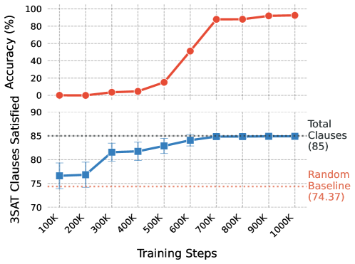
Figure 4: Evolution of the model’s SAT accuracy and number of satisfied clauses over training for random 3-SAT instances with $n=18$ on 185M model.

Figure 4 illustrates how the SAT accuracy evolves over training for a model trained on instances, showing for $n=18$ as a representative example. In the early stages (roughly the first half of training), the accuracy remains near zero, even as the model steadily improves in satisfying individual clauses. This indicates that the model initially learns partial solutions that satisfy a growing fraction of the clauses. Once the model begins consistently satisfying nearly all clauses in an instance, accuracy jumps sharply, reflecting that the assignments finally meet all the constraints simultaneously.

Appendix I Licenses and Copyrights Across Assets

1. PubLayNet Benchmark

   • Citation: (Zhong et al., 2019)

   • Asset Link: [link]

   • Lincense: [link]

2. RICO Benchmark

   • Citation:  (Deka et al., 2017)

   • Asset Link: [link]

   • License:[link]

3. QM9 Benchmark

   • Citation:  (Ramakrishnan et al., 2014)

   • Asset Link: [link]

   • License: [link]

4. Random 3-SAT benchmark

   • Citation:  (Ye et al., 2024)

   • Asset Link: [link]

   • License: [link]

5. PySAT: Python toolkit for prototyping with SAT solvers

   • Citation:  (Ignatiev et al., 2018)

   • Asset Link: [link]

   • License: [link]

References

- Austin et al. (2021) Austin, J., Johnson, D. D., Ho, J., Tarlow, D., and Van Den Berg, R. Structured denoising diffusion models in discrete state-spaces. Advances in Neural Information Processing Systems, 34:17981–17993, 2021.
- Chen et al. (2024) Chen, J., Zhang, R., Zhou, Y., and Chen, C. Towards aligned layout generation via diffusion model with aesthetic constraints. In The Twelfth International Conference on Learning Representations, 2024.
- Clarke et al. (2001) Clarke, E., Biere, A., Raimi, R., and Zhu, Y. Bounded model checking using satisfiability solving. Form. Methods Syst. Des., 19(1):7–34, July 2001. ISSN 0925-9856. doi: 10.1023/A:1011276507260.
- Cook (1971) Cook, S. A. The complexity of theorem-proving procedures. In Proceedings of the Third Annual ACM Symposium on Theory of Computing, STOC ’71, pp. 151–158, 1971.
- Deka et al. (2017) Deka, B., Huang, Z., Franzen, C., Hibschman, J., Afergan, D., Li, Y., Nichols, J., and Kumar, R. Rico: A mobile app dataset for building data-driven design applications. In Proceedings of the 30th annual ACM symposium on user interface software and technology, pp. 845–854, 2017.
- Ding et al. (2015) Ding, J., Sly, A., and Sun, N. Proof of the satisfiability conjecture for large k. In Proceedings of the Forty-Seventh Annual ACM Symposium on Theory of Computing, STOC ’15, pp. 59–68, 2015.
- Fuchs et al. (2020) Fuchs, F., Worrall, D., Fischer, V., and Welling, M. Se (3)-transformers: 3d roto-translation equivariant attention networks. Advances in neural information processing systems, 33:1970–1981, 2020.
- Gebauer et al. (2019) Gebauer, N., Gastegger, M., and Schütt, K. Symmetry-adapted generation of 3d point sets for the targeted discovery of molecules. In Advances in Neural Information Processing Systems 32. 2019.
- Gelfand & Smith (1990) Gelfand, A. E. and Smith, A. F. Sampling-based approaches to calculating marginal densities. Journal of the American statistical association, 85(410):398–409, 1990.
- Geman & Geman (1984) Geman, S. and Geman, D. Stochastic relaxation, gibbs distributions, and the bayesian restoration of images. IEEE Transactions on pattern analysis and machine intelligence, (6):721–741, 1984.
- Gomes et al. (2008) Gomes, C. P., Kautz, H., Sabharwal, A., and Selman, B. Satisfiability solvers. Foundations of Artificial Intelligence, 3:89–134, 2008.
- Guerreiro et al. (2025) Guerreiro, J. J. A., Inoue, N., Masui, K., Otani, M., and Nakayama, H. Layoutflow: flow matching for layout generation. In European Conference on Computer Vision, pp. 56–72. Springer, 2025.
- Gupta et al. (2021) Gupta, K., Lazarow, J., Achille, A., Davis, L. S., Mahadevan, V., and Shrivastava, A. Layouttransformer: Layout generation and completion with self-attention. In Proceedings of the IEEE/CVF International Conference on Computer Vision, pp. 1004–1014, 2021.
- Heusel et al. (2017) Heusel, M., Ramsauer, H., Unterthiner, T., Nessler, B., and Hochreiter, S. Gans trained by a two time-scale update rule converge to a local nash equilibrium. Advances in neural information processing systems, 30, 2017.
- Ho et al. (2020) Ho, J., Jain, A., and Abbeel, P. Denoising diffusion probabilistic models. Advances in neural information processing systems, 33:6840–6851, 2020.
- Hoogeboom et al. (2022) Hoogeboom, E., Satorras, V. G., Vignac, C., and Welling, M. Equivariant diffusion for molecule generation in 3d. In International conference on machine learning, pp. 8867–8887. PMLR, 2022.
- Hua et al. (2024) Hua, C., Luan, S., Xu, M., Ying, Z., Fu, J., Ermon, S., and Precup, D. Mudiff: Unified diffusion for complete molecule generation. In Learning on Graphs Conference, pp. 33–1. PMLR, 2024.
- Ignatiev et al. (2018) Ignatiev, A., Morgado, A., and Marques-Silva, J. PySAT: A Python toolkit for prototyping with SAT oracles. In SAT, pp. 428–437, 2018. doi: 10.1007/978-3-319-94144-8˙26. URL https://doi.org/10.1007/978-3-319-94144-8_26.
- Inoue et al. (2023) Inoue, N., Kikuchi, K., Simo-Serra, E., Otani, M., and Yamaguchi, K. Layoutdm: Discrete diffusion model for controllable layout generation. In Proceedings of the IEEE/CVF Conference on Computer Vision and Pattern Recognition, pp. 10167–10176, 2023.
- Jiang et al. (2023) Jiang, Z., Guo, J., Sun, S., Deng, H., Wu, Z., Mijovic, V., Yang, Z. J., Lou, J.-G., and Zhang, D. Layoutformer++: Conditional graphic layout generation via constraint serialization and decoding space restriction. In Proceedings of the IEEE/CVF Conference on Computer Vision and Pattern Recognition, pp. 18403–18412, 2023.
- Kikuchi et al. (2021) Kikuchi, K., Simo-Serra, E., Otani, M., and Yamaguchi, K. Constrained graphic layout generation via latent optimization. In Proceedings of the 29th ACM International Conference on Multimedia, 2021.
- Köhler et al. (2020) Köhler, J., Klein, L., and Noe, F. Equivariant flows: Exact likelihood generative learning for symmetric densities. In Proceedings of the 37th International Conference on Machine Learning, volume 119 of Proceedings of Machine Learning Research. PMLR, 2020.
- Landrum et al. (2006) Landrum, G. et al. Rdkit: Open-source cheminformatics, 2006.
- Lee et al. (2020) Lee, H.-Y., Jiang, L., Essa, I., Le, P. B., Gong, H., Yang, M.-H., and Yang, W. Neural design network: Graphic layout generation with constraints. In Computer Vision–ECCV 2020: 16th European Conference, Glasgow, UK, August 23–28, 2020, Proceedings, Part III 16, pp. 491–506. Springer, 2020.
- Levi et al. (2023) Levi, E., Brosh, E., Mykhailych, M., and Perez, M. Dlt: Conditioned layout generation with joint discrete-continuous diffusion layout transformer. In Proceedings of the IEEE/CVF International Conference on Computer Vision, pp. 2106–2115, 2023.
- Levin & Peres (2017) Levin, D. A. and Peres, Y. Markov chains and mixing times, volume 107. American Mathematical Soc., 2017.
- Loshchilov & Hutter (2019) Loshchilov, I. and Hutter, F. Decoupled weight decay regularization. In International Conference on Learning Representations, 2019. URL https://openreview.net/forum?id=Bkg6RiCqY7.
- Lou et al. (2023) Lou, A., Meng, C., and Ermon, S. Discrete diffusion language modeling by estimating the ratios of the data distribution. 2023.
- Martinelli (1999) Martinelli, F. Lectures on glauber dynamics for discrete spin models. Lectures on probability theory and statistics (Saint-Flour, 1997), 1717:93–191, 1999.
- Meng et al. (2021) Meng, C., He, Y., Song, Y., Song, J., Wu, J., Zhu, J.-Y., and Ermon, S. Sdedit: Guided image synthesis and editing with stochastic differential equations. arXiv preprint arXiv:2108.01073, 2021.
- Meng et al. (2022) Meng, C., Choi, K., Song, J., and Ermon, S. Concrete score matching: Generalized score matching for discrete data. Advances in Neural Information Processing Systems, 35:34532–34545, 2022.
- OpenAI (2024) OpenAI. Learning to reason with llms, 2024. URL https://openai.com/index/learning-to-reason-with-llms/.
- Peebles & Xie (2023) Peebles, W. and Xie, S. Scalable diffusion models with transformers. In Proceedings of the IEEE/CVF International Conference on Computer Vision, pp. 4195–4205, 2023.
- Peng et al. (2023) Peng, X., Guan, J., Liu, Q., and Ma, J. Moldiff: Addressing the atom-bond inconsistency problem in 3d molecule diffusion generation. In International Conference on Machine Learning, pp. 27611–27629. PMLR, 2023.
- Radford et al. (2019) Radford, A., Wu, J., Child, R., Luan, D., Amodei, D., Sutskever, I., et al. Language models are unsupervised multitask learners. OpenAI blog, 1(8):9, 2019.
- Ramakrishnan et al. (2014) Ramakrishnan, R., Dral, P. O., Rupp, M., and Von Lilienfeld, O. A. Quantum chemistry structures and properties of 134 kilo molecules. Scientific data, 1(1):1–7, 2014.
- Rombach et al. (2022) Rombach, R., Blattmann, A., Lorenz, D., Esser, P., and Ommer, B. High-resolution image synthesis with latent diffusion models. In Proceedings of the IEEE/CVF conference on computer vision and pattern recognition, pp. 10684–10695, 2022.
- Saharia et al. (2022) Saharia, C., Chan, W., Saxena, S., Li, L., Whang, J., Denton, E. L., Ghasemipour, K., Gontijo Lopes, R., Karagol Ayan, B., Salimans, T., et al. Photorealistic text-to-image diffusion models with deep language understanding. Advances in neural information processing systems, 35:36479–36494, 2022.
- Song et al. (2020) Song, Y., Sohl-Dickstein, J., Kingma, D. P., Kumar, A., Ermon, S., and Poole, B. Score-based generative modeling through stochastic differential equations. arXiv preprint arXiv:2011.13456, 2020.
- Turchin (1971) Turchin, V. F. On the computation of multidimensional integrals by the monte-carlo method. Theory of Probability & Its Applications, 16(4):720–724, 1971.
- Varma et al. (2024) Varma, H., Nagaraj, D., and Shanmugam, K. Glauber generative model: Discrete diffusion models via binary classification. arXiv preprint arXiv:2405.17035, 2024.
- Vignac et al. (2023a) Vignac, C., Krawczuk, I., Siraudin, A., Wang, B., Cevher, V., and Frossard, P. Digress: Discrete denoising diffusion for graph generation. In The Eleventh International Conference on Learning Representations, 2023a. URL https://openreview.net/forum?id=UaAD-Nu86WX.
- Vignac et al. (2023b) Vignac, C., Osman, N., Toni, L., and Frossard, P. Midi: Mixed graph and 3d denoising diffusion for molecule generation. In Joint European Conference on Machine Learning and Knowledge Discovery in Databases, pp. 560–576. Springer, 2023b.
- Vizel et al. (2015) Vizel, Y., Weissenbacher, G., and Malik, S. Boolean satisfiability solvers and their applications in model checking. Proceedings of the IEEE, 103(11):2021–2035, 2015.
- Wei et al. (2022) Wei, J., Wang, X., Schuurmans, D., Bosma, M., Xia, F., Chi, E., Le, Q. V., Zhou, D., et al. Chain-of-thought prompting elicits reasoning in large language models. Advances in neural information processing systems, 35:24824–24837, 2022.
- Xu et al. (2019) Xu, J., Sun, X., Zhang, Z., Zhao, G., and Lin, J. Understanding and improving layer normalization. In Advances in Neural Information Processing Systems, volume 32, 2019. URL https://proceedings.neurips.cc/paper_files/paper/2019/file/2f4fe03d77724a7217006e5d16728874-Paper.pdf.
- Xu et al. (2023) Xu, M., Powers, A. S., Dror, R. O., Ermon, S., and Leskovec, J. Geometric latent diffusion models for 3d molecule generation. In International Conference on Machine Learning, 2023.
- Ye et al. (2024) Ye, J., Gao, J., Gong, S., Zheng, L., Jiang, X., Li, Z., and Kong, L. Beyond autoregression: Discrete diffusion for complex reasoning and planning. arXiv preprint arXiv:2410.14157, 2024.
- Zhang et al. (2023) Zhang, J., Guo, J., Sun, S., Lou, J.-G., and Zhang, D. Layoutdiffusion: Improving graphic layout generation by discrete diffusion probabilistic models. In Proceedings of the IEEE/CVF International Conference on Computer Vision, pp. 7226–7236, 2023.
- Zhang et al. (2024) Zhang, Y., Yang, D., and Liao, R. Symmetricdiffusers: Learning discrete diffusion on finite symmetric groups. arXiv preprint arXiv:2410.02942, 2024.
- Zhong et al. (2019) Zhong, X., Tang, J., and Yepes, A. J. Publaynet: largest dataset ever for document layout analysis. In 2019 International Conference on Document Analysis and Recognition (ICDAR), 2019. doi: 10.1109/ICDAR.2019.00166.