Semi-supervised classification of bird vocalizations

Abstract

Changes in bird populations can indicate broader changes in ecosystems, making birds one of the most important animal groups to monitor. Combining machine learning and passive acoustics enables continuous monitoring over extended periods without direct human involvement. However, most existing techniques require extensive expert-labeled datasets for training and cannot easily detect time-overlapping calls in busy soundscapes. We propose a semi-supervised acoustic bird detector designed to allow both the detection of time-overlapping calls (when separated in frequency) and the use of few labeled training samples. The classifier is trained and evaluated on a combination of community-recorded open-source data and long-duration soundscape recordings from Singapore. It achieves a mean $F_{0.5}$ score of 0.701 across 315 classes from 110 bird species on a hold-out test set, with an average of 11 labeled training samples per class. It outperforms the state-of-the-art BirdNET classifier on a test set of 103 bird species despite significantly fewer labeled training samples. The detector is further tested on 144 microphone-hours of continuous soundscape data. The rich soundscape in Singapore makes suppression of false positives a challenge on raw, continuous data streams. Nevertheless, we demonstrate that achieving high precision in such environments with minimal labeled training data is possible.

[inst1]organization=ARL, Tropical Marine Science Institute, National University of Singapore [inst2]organization=Department of Electrical & Computer Engineering, National University of Singapore [inst3]organization=National Parks Board, country=Singapore

1 Introduction

Biodiversity monitoring is a critical aspect of biodiversity conservation, as it helps inform decision making, improves our knowledge and enhances public education and awareness. Birds are one of the most surveyed animal groups in biodiversity monitoring programmes, with point counts and transect surveys being well-established survey techniques for monitoring bird communities [1]. However, birds can be very difficult to detect and identify especially in tropical regions characterised by high avian diversity and numerous rare species [2], [3]. Additionally, such manned survey techniques are manpower-intensive, require highly specialized expertise, and tend to overlook rare species that are sensitive to human presence [4], [5], [6].

Passive monitoring of biodiversity using acoustics is thus an area of great potential, as various animal groups including birds make unique vocalizations, which can be used to validate their presence. Such systems allow for automated collection of large amounts of audio data without human supervision and can survey cryptic species more effectively [4], [7]. However, the comprehensive analysis of such large volumes of data is prohibitive in terms of the man-hours required [8]. This constraint, and the rapid advancement in machine learning techniques, have made data-driven algorithms increasingly popular for bioacoustic species detection and classification tasks. The dominant approach in this space involves feeding time-frequency spectrograms of acoustic recordings to some variant of a Convolutional Neural Network for feature extraction and classification [9]. What many of these methods have in common, however, is the need for extensive sets of expert-labeled training data. As an example, the initial BirdNET classifier [10] was trained to classify close to 1000 different bird species but with about 1,500 spectrograms per class on average. The general need for large datasets may in part be attributed to the excessive information present in broadband spectrograms, which requires the model to learn to distinguish the signal of interest from the noise, and in part because many labeled datasets used for training are weakly labeled, i.e., class labels are typically assigned at spectrogram level without information about the exact time and frequency of the event. Transfer learning has emerged as a common technique to address the shortage of task-specific data. The idea is to improve a model’s performance on a specific task by leveraging knowledge gained from a model previously trained on a different but related task. In acoustic classification, it is common to leverage models pre-trained on large datasets of either images or generic audio (typically ImageNet [11] or AudioSet [12]), and fine-tune these networks on task-specific data [13], [14], [15]. Although transfer learning can be effective, one is constrained by the architecture and input format of the pre-trained models, which may be suboptimal for the target task. Models pre-trained on ImageNet, for example, typically require inputs of size $224\times 224\times 3$, constraining the selection of duration, bandwidth, and time-frequency resolution of the spectrograms. A different but closely related approach, known as meta-learning, trains a model on a set of different tasks with the aim to generalize to new tasks with very few training samples. Several promising few-shot learning approaches on bioacoustic data are presented in [16], but one still needs to curate a labeled dataset on a diverse set of tasks to train the initial model before the few-shot learning can take place.

How to handle soundscapes with temporally-dense vocalizations is another challenge in bioacoustics. This is particularly relevant for birds, as many bird species are especially vocal during dawn and dusk, resulting in vocalization-dense soundscapes with frequent time-overlapping calls. One approach is to train multi-label classifiers, i.e., classifiers that can predict multiple target classes from a single input. Multi-labeled datasets, however, as compared to single-labeled datasets, are far less prevalent, harder and more tedious to accurately annotate [17], and, as a consequence, are not always exhaustive, which can inhibit learning [18]. Moreover, multi-label classification requires more training data because the problem is inherently harder. The lack of large, high-quality multi-labeled datasets in bioacoustics may be one reason why most research focuses on single-labeled problems (e.g. [19], [20], [21], [16], [14]). Methodologies targeting multi-label classification tend to divide spectrograms into shorter windows, apply classifiers (either single-label or multi-label) to each window, and aggregate the outputs to obtain predicted scores for all species present in the full spectrogram [10], [13], [22]. The motivation behind this split-and-aggregate strategy is likely to increase the chance of capturing single vocalizations at a time, which reduces the multi-label problem to a set of single-label problems. A shortcoming of this approach, however, is that the models are fed spectrograms of fixed duration and bandwidth, while the duration and bandwidth of vocalizations vary, effectively including excessive information and allowing time-overlapping calls to enter the same input. In [17], the authors address this issue by employing a supervised, pixel-level segmentation technique to separate calls in time and frequency prior to classification. This method, however, requires labeled training data for both segmentation and classification. In [23], an object detection technique was used to detect marine mammals acoustically. Although this approach can detect time-overlapping vocalizations, it requires hard labels in the form of bounding boxes enclosing the signals of interest. This, and other labour-intensive annotation processes, may be acceptable if the objective is to detect a few specific vocalizations, but does not scale well to the vast diversity of bird vocalizations.

Lastly, most studies to date in the field of passive acoustics monitoring have involved largely pristine habitats while urban ecosystems have largely been overlooked [24], [25]. As urban green spaces become increasingly important for bird populations due to the rapid rate of urbanisation [26], evaluating the efficacy of utilising automated analysis for urban soundscapes is particularly urgent. The highly urbanised city-state of Singapore is an ideal study site as it is one of the few tropical cities that has a network of connected urban green spaces close to densely populated urban areas [27].

To target these challenges, we propose a semi-supervised, passive-acoustic bird classifier designed to allow detection of time-overlapping vocalizations (when separated in frequency) without requiring a large number of labeled data for training. We assess its performance on both open-source recordings from Singapore and long-duration, continuous soundscape data recorded at two different sites within the Singapore Botanic Gardens (SBG) – one of the oldest botanic gardens in Southeast Asia which receives millions of visitors annually.

2 Methodology

The proposed method consists of four main steps which are explained in detail in the remainder of this section:

1. Segmentation: extract individual bird calls with an energy-based segmentation technique. The isolation of individual bird calls limits noise, enabling high data compression, and allows time-overlapping calls to be treated separately as long as they do not also overlap in frequency. A consequence of this approach is that single calls/songs may be split into multiple segments.

2. Data compression: learn a compressed representation of the segments while retaining most of the information.

3. Embedding: use the representation from step 2 to learn a new representation (embedding) to ensure both translational invariance and that similar sounds have similar embedding – two key properties for efficient clustering and classification.

4. Classification: curate a set of labeled data and train a classifier using the embeddings from step 3. This training process also serves as a final refinement of the embedding.

Note that step 1 does not involve any learning and step 2 and 3 are self-supervised, i.e., no labeled data is required. Training the self-supervised networks on large datasets allows the supervised classifier in the final step to distinguish the classes with a much smaller set of labeled data.

2.1 Data collection

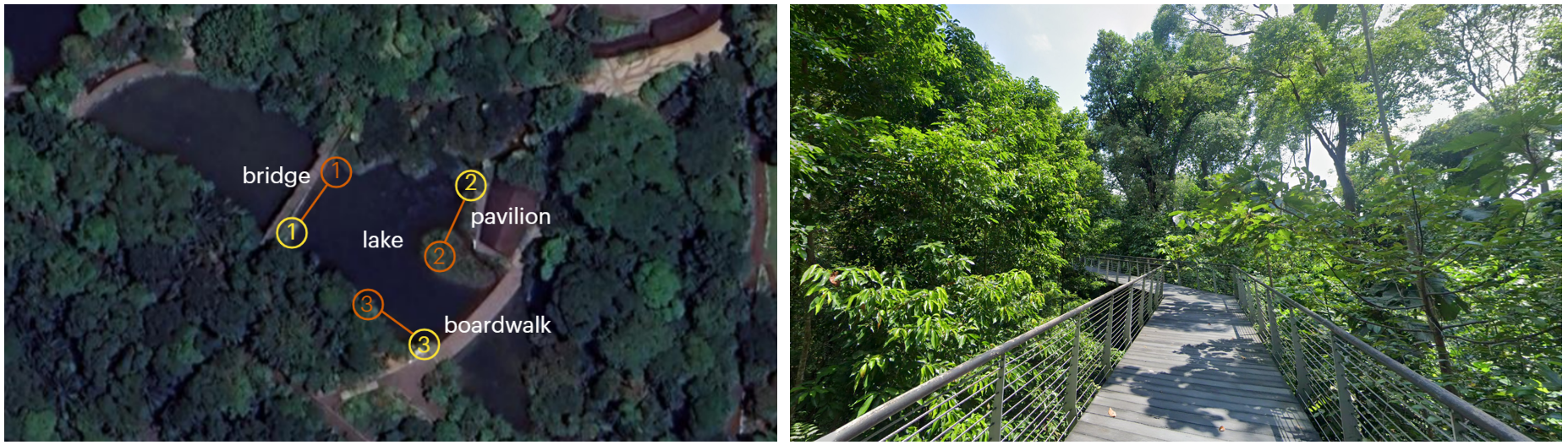
Figure 1: Left: first deployment at the SBG (site #1) from July 4, 2020 until September 20, 2020. The approximate locations of the recording units are marked as yellow circles, with the corresponding external microphones of each unit marked as orange circles. The 6 microphones surround a lake and cover an area of roughly 50 m $\times$ 50 m. Right: a section of the elevated boardwalk used for the second deployment at the SBG (site #2) from September 20, 2020 until February 1, 2021. The same 6 microphones from site #1 were deployed along the circular boardwalk in a similar constellation, but without direct line of sight between units due to the dense vegetation. Photos from Google Maps.

Our primary source of acoustic data was acquired from two different locations in the SBG over a combined period of 7 months from July 2020 to February 2021. Three Wildlife Acoustics SongMeter 4 TS recorders were deployed at both locations. Each recording unit was equipped with two omni-directional microphones, yielding soundscape recordings from 6 microphones simultaneously. The first 2.5 months of data collection took place around a lake with minimal obstruction between the microphones (site #1). This setup allows the same call to be detected on multiple recorders (Figure 1), which we later leverage to train the contrastive network (Subsection 2.4). The units were then re-located to a second site for the remaining 4.5 months (site #2). A similar constellation was used but dense vegetation occluded the direct paths between microphones (Figure 1). During calibration tests at site #2, we emitted high-energy, transient sounds and found that the sounds were mostly audible only on the nearest few microphones. Although low-frequency sounds may attenuate less, site #2 is likely to have a significantly lower detection range.

Lastly, the collected soundscape recordings were complemented with 333 carefully selected bird recordings of species known to be present in Singapore from the Xeno-canto database. These community-curated recordings served as a faster way to obtain an initial set of local bird calls without having to search in long, unprocessed recordings.

2.2 Time-frequency representation

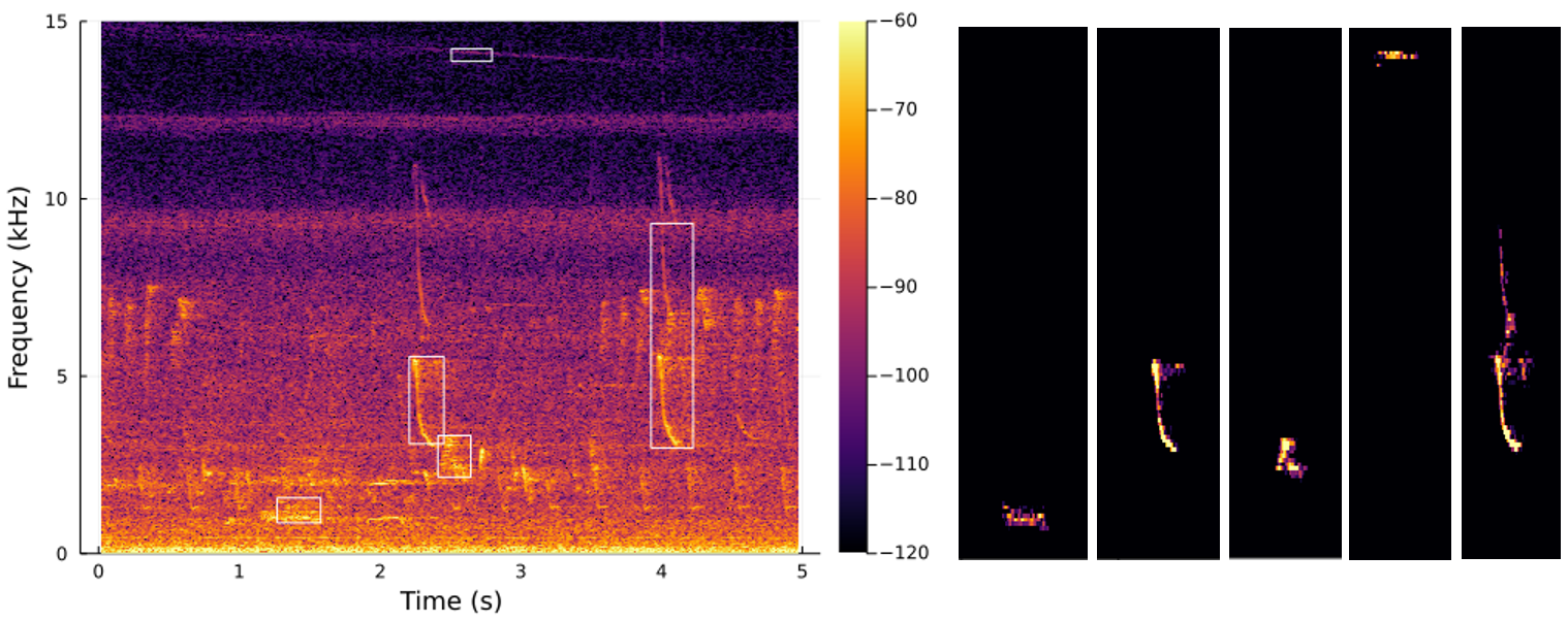
Figure 2: An example illustrating extraction of TFRs from audio recordings. The left panel shows the spectrogram from a 5 second audio clip, with a few detected sounds enclosed by white rectangles. The right panels show the respective extracted TFRs. This example is non-exhaustive, i.e., not all detections in the audio clip are shown here.

Most bird vocalizations contain time-frequency transients. While vocalizations may overlap in time, they may be separated in frequency. Based on this observation, time-frequency transients are extracted from acoustic recordings as the initial stage of the technique. The extracted time-frequency transients are represented as a $128\times 256$ matrix of numbers referred to as the time-frequency representation (TFR). TFRs are extracted from acoustic recordings through the following steps:

1. Compute a spectrogram of the acoustic data with 2,048 FFT bins, a Hamming window, and an overlap of 1,536 samples between windows. Retain the frequency bins between 500 Hz and 15 kHz only, as this frequency range adequately covers most bird sounds while rejecting other unwanted noises.

2. Convert the spectrogram to dB. Using the inter-quartile range for each frequency bin to obtain a robust estimate of the noise variance $\sigma$ at that frequency. Normalize each frequency bin by subtracting the median + $2\sigma$, dividing by $2\sigma$, and lastly clipping the resulting data between 0 and 1. This adaptively extracts regions in the time-frequency plane that have significantly higher energy than the background noise at that frequency. Moreover, it reduces the natural dominance of low-frequency calls resulting from higher attenuation of high-frequency signals [28].

3. Reduce the frequency resolution by a factor of 5 by max-pooling.

4. Blank out time bins with low variance across broad frequency bands, as these represent impulsive sounds not characteristic of birds.

5. Perform a watershed segmentation of the resulting spectrogram to obtain disconnected regions of high energy in the spectrogram.

6. Filter out regions with very short durations or very small time-bandwidth products, as these are uncharacteristic of bird sounds.

The end result of the above steps is best illustrated through an example (Figure 2). The spectrogram on the left is from a 5 second long recording with multiple bird vocalizations. After going through the above steps, the spectrogram is converted to a number of TFRs. A few of these TFRs are shown in the panels on the right with corresponding sections marked with white rectangles in the original spectrogram on the left.

Although the TFR representations have variable duration, many of the algorithms used in our signal processing chain require a constant duration input. We pick a constant duration of 2.7 seconds (256 time bins for the TFR), and convert all TFRs to this duration when feeding to algorithms that require a constant duration input. This duration is sufficient to cover most of the TFRs we obtain. For the occasional TFR longer than 2.7 seconds, we randomly select a 256-sample section, while shorter TFRs are randomly zero-padded on both sides to make them 256 samples long. The random padding or clipping is done on the fly to create different versions of the TFR each time it is used. Note that in contrast to methods that operates on entire spectrograms, the complexity level of the downstream classification task is not impacted by the call density as long as single TFRs do not capture multiple calls.

2.3 Auto-encoding

While TFRs may be a good visual representation for humans to classify bird vocalizations, it is not necessarily a good representation for a machine. The TFRs are also generally sparse, with most entries containing zero energy. The auto-encoder stage of the processing learns a compressed representation of the TFR that retains most of the information from the original TFR, but using a much smaller number of coefficients. The learning is self-supervised, i.e., no labeled data is required. The auto-encoder simply seeks to reduce the error between the original TFR and a reconstructed TFR with the constraint that the intermediate representation of the TFR (the latent representation) only contains 512 values (instead of the $128\times 256$ values in the original input TFR).

We use a convolutional deep auto-encoder to achieve this compression (Figure 3). To train the auto-encoder we build a dataset of TFRs extracted from about 90 microphone-hours of recordings, primarily from the two SBG locations and a smaller subset obtained from the Xeno-canto recordings. To encourage the model to emphasize learning of bird sounds over sounds from other sources, we additionally add three identical sets of the curated TFRs which we later use to train the final classifier (Subsection 2.5). This brings the final count to 228,042 TFRs. From these, 5,000 TFRs are used for validation and the balance 223,042 TFRs for training. We use a mean-square error loss function and train the auto-encoder over 97 epochs using the Adam optimizer [29]. The auto-encoder is capable of retaining most of the information in the TFRs, as illustrated in Figure 4. After training, the encoder section of the auto-encoder is kept and used as a pre-trained, second-stage processor for the remaining stages of the algorithm.

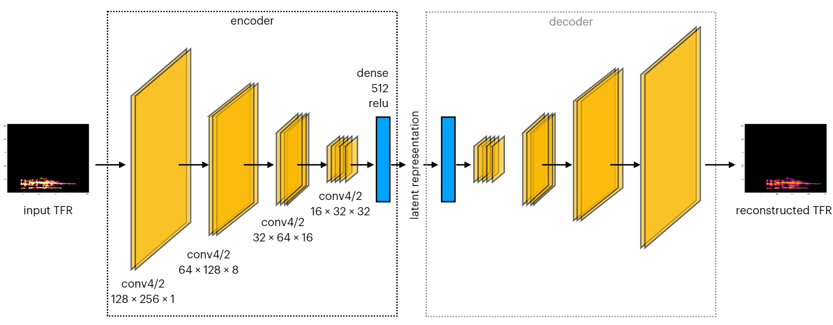
Figure 3: Architecture of the convolutional auto-encoder. The network enables a $64\times$ data compression by learning a latent representation of the TFRs which retains most of the information.

2.4 Contrastive representation learning

While the latent representation from the previous section holds information related to bird vocalization in a compressed form, it is not a suitable representation for clustering or classification tasks. Firstly, auto-encoder latent spaces are translation equivariant, i.e., when the input TFR is shifted in time, the output TFR also shifts in time. To do this, the latent representation must retain time information. However, a bird sound shifted in time doesn’t change the bird, and so we seek translation invariance rather than translation equivariance. Secondly, very similar sounds can have very different latent space representations, as nothing in the training process impose any constraint to force similar sounds to have similar representations. We next use the idea of contrastive learning to discover a preliminary embedding that is invariant to time translation and where similar sounds have similar representations.

Traditional contrastive learning [30] obtains a pair of samples from each training sample by augmenting the training sample in two different ways. The pair is thus guaranteed to be similar, but not the same. Training the contrastive learning network then involves the design of a loss function that requires the samples in each pair to have similar representations, but samples from different pairs to differ as much as possible. This permits self-supervised training without the need for labeled samples, and the network learns a representation that is invariant to the augmentation used to create a pair of samples.

We follow the same basic approach outlined above, but change some of the details in some critical ways. Other than a random translation that is inherent in obtaining a TFR of constant duration (Subsection 2.2), we do not perform any augmentation. Instead, sample pairs are derived from recordings of the same bird vocalization on the two microphones connected to each recorder unit. The natural variability in sound propagation thus provides the desired “augmentation”. Since the sound reaches both microphones at potentially different times, some effort is required to associate the sounds on both microphones. Using a combination of time information and a requirement for high cross-correlation between the acoustic time-series of both sounds, we obtain 19,311 reliable TFR pairs from the two SBG deployments. Of these, 500 pairs are used for validation and the balance 18,811 for training. The contrastive learning network outputs a learnt representation space referred to as the embedding space hereafter (Figure 5). The training is performed over 50 epochs using the Adam optimizer, but with a loss function that is different from the one proposed in [30].

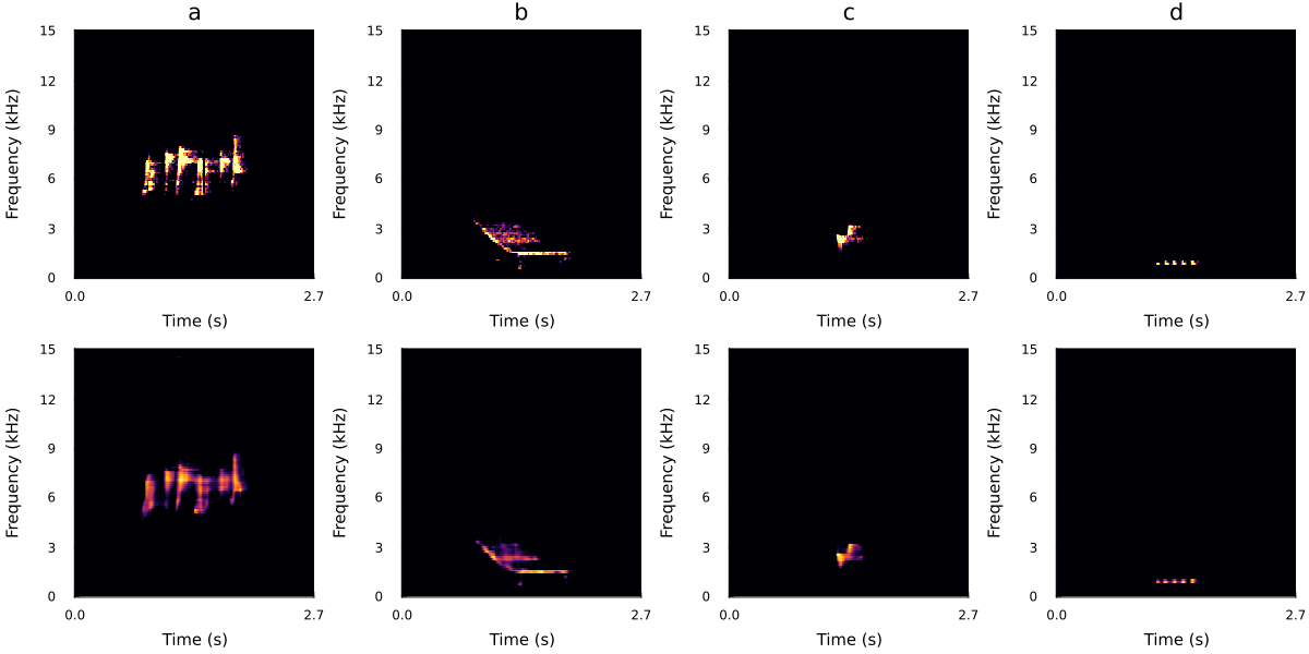
Figure 4: Examples of calls from (a): Crimson Sunbird (Aethopyga siparaja, 558466), (b): Common Hill Myna (Gracula religiosa, 179652), (c): Olive-winged Bulbul (Pycnonotus plumosus, 562623) and (d): Lineated Barbet (Psilopogon lineatus, 1145226). The top row shows the TFRs after extraction from raw audio recordings, and the bottom row shows the compressed TFRs after passing through the auto-encoder. The high similarity between each pair shows that the compressed latent representation is capable of retaining most of the information in the TFRs. To limit sounds from different sources from merging, TFRs do not capture entire calls/songs if the pause between subsequent vocalizations are too long. The Olive-winged Bulbul in column c is one such example, where only a part of a longer call sequence is captured.

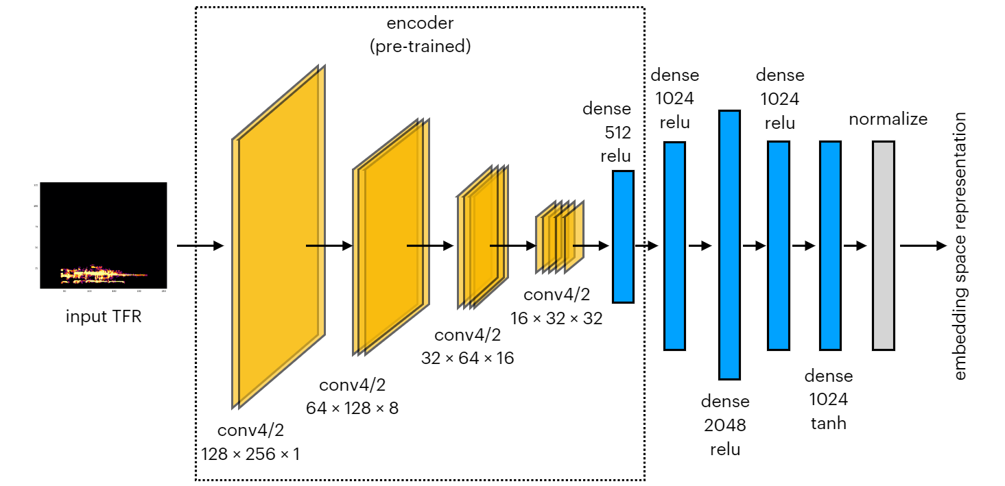
Figure 5: Architecture of the contrastive learning neural network. The $\tanh(\cdot)$ activation function in the last dense layer ensures all entries in the 1024-dimensional embedding space representation are positive, and the final normalization layer ensures that they are scaled such that the embedding space can be thought of as the surface of a hypersphere of unit radius. The similarity between embedding space representations can then be measured in terms of the dot product of the corresponding vectors. The distance between embedding space representations can be measured as the angle between vectors, or equivalently the distance on the surface of the hypersphere.

Although the loss function proposed in [30] is theoretically sound, it was developed for a computer vision task quite different from our needs and did not perform well on our problem. Based on the intuition that the embedding space can be modeled as a surface of a 1024-dimensional hypersphere, we do not desire maximal angular separation between dissimilar sounds, but rather orthogonality. Maximal angular separation pushes dissimilar sounds to diametrically opposite sides of the hypersphere, but that can only accommodate two classes. Instead, orthogonality pushes dissimilar sounds to different axes of the hypersphere, and can support up to 1024 distinct classes for a 1024-dimensional hypersphere. With this in mind, the loss function we use is:

$$L(\mathbf{Z}) = \sum_{p=1}^{N}l_{2p,2p-1}+l_{2p-1,2p},$$ (1)

$$l_{i,j} = -\left[\mathbf{z}_{i}^{T}\mathbf{z}_{j}+\beta\sum_{k\neq i,k\neq j}^{2N}\min\left(1-\mathbf{z}_{i}^{T}\mathbf{z}_{k},\;1\right)^{2}\right].$$ (2)

Here $\mathbf{Z}=\{\mathbf{z}_{i}\forall i\}$ is the set of embedding space representations for the training TFRs, organized such that the first pair is $(\mathbf{z}_{1},\mathbf{z}_{2})$, the second pair is $(\mathbf{z}_{3},\mathbf{z}_{4})$, and so on. The two terms in (1) correspond to two possible orderings of samples in each pair. The first term in (2) maximizes the similarity within each pair, while the second term induces orthogonality for non-paired representations. The $\min(\cdot,1)$ function prevents maximal angular separation and $\beta=3$ is a hyper-parameter that controls the balance between the two terms. In practice, the loss is not evaluated over the entire dataset, but in mini-batches of $N=512$.

After training, an average similarity score $\mathbf{z}_{i}^{T}\mathbf{z}_{j}$ of 0.93 was obtained for paired samples, and near orthogonality for non-paired samples. While this ensures that paired samples (similar sounds) have high similarity, it does not guarantee low similarity between every pair of dissimilar sounds. Since the loss function minimizes the average similarity between dissimilar sounds, some clusters of dissimilar sounds still experience very similar representations. This is addressed by allowing the embedding space representation to further improve in a final, supervised classification stage.

2.5 Supervised refinement and classification

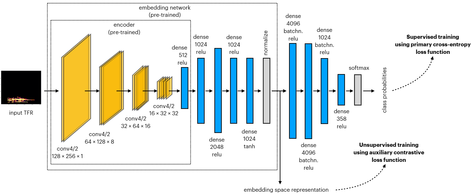
Figure 6: The complete classification architecture. TFRs extracted from raw recordings are transformed to compressed embedding vectors via a pre-trained auto-encoder followed by a pre-trained contrastive network. These embeddings vectors are then fed as input to a 4-layer classification network (right), which in turn assigns confidence scores to each predefined class. To allow the embedding network to improve further, its model parameters are not frozen during the final, supervised classification training. However, to ensure the embedding network does not forget its primary objective, it is trained once for every 5 epochs of classification training.

The final stage of the model is a classifier with four dense layers and batch normalization between each layer. It takes the preceding embedding vector as input and assigns a confidence score to each predefined class (Figure 6). As a single species can produce a wide range of calls with very different time-frequency representations, and since the preceding contrastive network operates on compressed TFRs from the auto encoder, the classifier is trained at TFR-level rather than at species-level. Consequently, the classifier does not only learn to differentiate between species but also between different calls from same species. However, TFRs are not guaranteed to capture entire call sequences. As a result, single calls or songs are sometimes fragmented into multiple TFRs and, in turn, assigned to separate classes if significantly distinct.

About 2/3 of the training data is obtained by extracting TFRs from Xeno-Canto files which are first manually labeled. These recordings are typically characterized by high SNR and are relatively short in duration (tens of seconds to a few minutes long), resulting in few but very clean samples for many classes. These clean samples, however, are not necessarily representative of the chaotic soundscape during peak chorus hours. The remaining 1/3 of the data is obtained by applying the pre-trained embedding network (Subsection 2.4) to search for clusters of similar TFRs in soundscape recordings from the two SBG sites. The embedding enables an efficient labeling process as whole clusters can be labeled by inspecting only a few samples. Classes with less than 3 samples are discarded, resulting in 5727 TFRs distributed over 357 classes, representing 123 bird species. The dataset, however, is highly imbalanced. While most classes only have a handful of samples, others have hundreds. When splitting the dataset into training, validation and test sets, we prioritize TFRs for training while ensuring that each class has at least one validation and one test sample. To account for the class imbalance, we randomly augment original TFRs from low-sample classes with minor shifts in frequency, minor time stretching, and by adding Gaussian and white noise, obtaining a balanced distribution with exactly 50 samples per class for training, and a minimum of 20 samples each for validation and testing.

The classifier will only extract and learn the necessary features from the input in order to separate the classes in the training set and minimize the cost function. When applying the model on continuous field recordings, however, the model is exposed to a much greater variety of sounds than it has seen during training, many of which will have very similar embeddings as some of the sounds from the trained classes. To make the model more robust against false positives in such environments, two additions to the algorithm are made. First, a separate bird-pass filter is trained to distinguish bird sounds from generic non-bird sounds. This binary classifier has three dense layers, takes encoded TFRs from the auto-encoder as input and classify them as either birds or non-birds. The training data for the bird class is the same as for the main classifier, while the non-bird class is trained on 3152 TFRs extracted primarily from the UrbanSound8K dataset [31] and in part from underwater recordings of marine mammal vocalizations, previously collected in Singapore waters. To avoid class imbalance, the non-bird sounds are oversampled with random frequency shifts to match the same sample size as the bird class. As even a small false positive rate can translate to a large number of false positives in raw recordings, we value precision over recall for bird classes. To encourage this precision-recall trade-off in the bird-pass filter, false positives are penalized more for the bird class than for the non-bird class, yielding a $F_{0.5}$ score of 0.91 for the bird class on a hold-out test set.

Secondly, an additional “sink” class is added to the primary classifier. Since most of the non-bird sounds used to train the bird-pass filter are unlikely to be present in our local environment, the sink class is trained on local sounds from the SBG. Specifically, it is trained with 1893 TFRs from site #1 which initially confused the model and caused many false positives. The sink class helps the model to learn lower-level features for classes which are easily confused with other local sounds, while also providing the neural network with a class to assign TFRs that do not belong to any of the trained bird classes. We use a standard cross-entropy loss function for the main classifier, but we penalize false negatives for the sink class by an effective factor of $3\times$ that of the bird classes, to discourage sink samples from being misclassified as birds.

Lastly, to address the challenge that some clusters of dissimilar sounds occur close in embedding space (Subsection 2.4), the classifier is trained end-to-end without freezing any of the preceding layers. This allows both the auto-encoder and the contrastive learning network to improve further. During this training, however, the trained embedding network can “forget” the need for paired samples to have high similarity and unpaired samples to have low average similarity. To reinforce this need, we simultaneously train the embedding network with the same contrastive loss as before (Subsection 2.4). In practice the training is implemented in sets of 5 epochs of the primary cross-entropy loss, followed by 1 epoch of the auxiliary contrastive loss. We train the network over 95 such sets and retain a mean similarity score of 0.866 for paired samples and near orthogonality (0.046) for unpaired samples.

3 Results

We evaluate the performance of the classifier in two settings. First, we assess its performance on a test set that neither the auto-encoder, the contrastive network, nor the classifier have encountered during training. We also compare the test set performance with the prevailing open-source acoustic bird detector, BirdNET [10]. Secondly, we assess how the model performs on raw, continuous soundscape recordings from the SBG to better understand its capabilities and limitations when deployed for extensive periods of time in a typical monitoring setup.

3.1 Evaluation on test set

Table 1: Classification performance on the test set.

	Bird classes	Sink class
Number of classes	315	1
Total test samples	6435	200
Precision	0.799	0.076
Recall	0.585	0.870
$F_{0.5}$	0.701	0.093

Although the TFR samples in each class originate from the same call category, there may still be individual variations, e.g. in duration (particularly for repetitive calls), bandwidth, and frequency modulation rate (for example the steepness of up- and downsweeps). Disturbances from extraneous sources, differences in SNR levels, and artifacts from the data augmentation process can further add to the TFR variation within each class. For classes with many training samples, such diversity can enhance the model’s capability to generalize as it forces the model to identify the distinguishing features of each class while ignoring irrelevant information. However, many of our classes have very few training samples, so when evaluating the model on the test set, we do not consider classes where most test samples differ significantly from the training. This reduces the test set to 315 bird classes across 110 species. Moreover, we assign low-confidence predictions (confidence scores below 0.5) to the sink class, which serves as a collector of extraneous TFRs. The sink class precision is consequently low, but more importantly, it obtains a high recall of 0.870, meaning that only 13% of the sink samples are misclassified as birds (Table 1). The bird classes achieve a mean $F_{0.5}$ score of 0.701 with a desirable asymmetry between precision (0.799) and recall (0.585). The performance for individual bird classes, however, is skewed: 37 classes have a $F_{0.5}$ score of 0.0 while 111 classes have a $F_{0.5}$ score above 0.9. The zero-score classes fall primarily into one or more of the following categories: 1) correct class but low confidence, 2) class not learned during training, i.e., $F_{0.5}=0.0$ on the training set, 3) confusion with similar classes, or 4) low similarity between test and training samples.

3.2 Comparison with BirdNET

To benchmark the model, we compare its performance against the BirdNET classifier [10]. BirdNET is a leading open-source acoustic bird detector, extensively used by bird enthusiasts and researchers worldwide, and it currently covers more than 6,000 bird species [32]. We use the same test set as in Subsection 3.1 for evaluation but differences between the two models require some adjustments. First, we consider only non-augmented samples. Second, as BirdNET is trained to detect species, we also evaluate our model at species-level rather than at TFR-level. Lastly, we exclude the few species that BirdNET is not trained to detect. The resulting test set consists of 943 samples from 103 species. The number of samples per species ranges from 1 to 101, with a median of 3 samples, meaning that only a handful of samples are available for most species. All samples lie within the 0-15 kHz frequency range covered by BirdNET.

We test the latest BirdNET version available via the Python Package Index (PyPi) repository [33] (version 0.1.6, released September 4, 2024). While our model takes TFRs as input (isolated in time and frequency), BirdNET searches for detections in broadband spectrograms. To reduce the probability of capturing multiple species in the recordings fed to BirdNET, we feed it 3-second-long raw recordings centered at each TFR (i.e., the minimum input duration that avoids signal padding). Since we have only ground truth annotations at TFR-level, we cannot guarantee that other species are absent from the 3-second recordings. However, BirdNET predicts between 0 and 7 species with confidence scores above 0.1 across the test set , with an average of 1.3 species, suggesting that multi-species presence is not a substantial issue. Nevertheless, as some samples may contain multiple species, we compare the models using top-k accuracy with $k=1$ and $k=3$, i.e., we consider a prediction correct as long as one of the top-k predictions (ranked by confidence score) matches the ground-truth. We evaluate the mean top-1 and top-3 accuracy, both globally (where each sample is weighted equally) and species-averaged (where each species class is weighted equally) to account for the sample imbalance between species (Table 2). Our model achieves significantly higher accuracy than BirdNET across all metrics on the test set, despite half of the 103 species are trained with less than 16 labeled samples each.

Table 2: Performance comparison between BirdNET and our model on 943 test samples across 103 species.

	BirdNET	Our model
Top-1 accuracy	0.51	0.81
Top-3 accuracy	0.66	0.89
Top-1 accuracy (species-averaged)	0.50	0.73
Top-3 accuracy (species-averaged)	0.64	0.82

3.3 Evaluation on continuous data

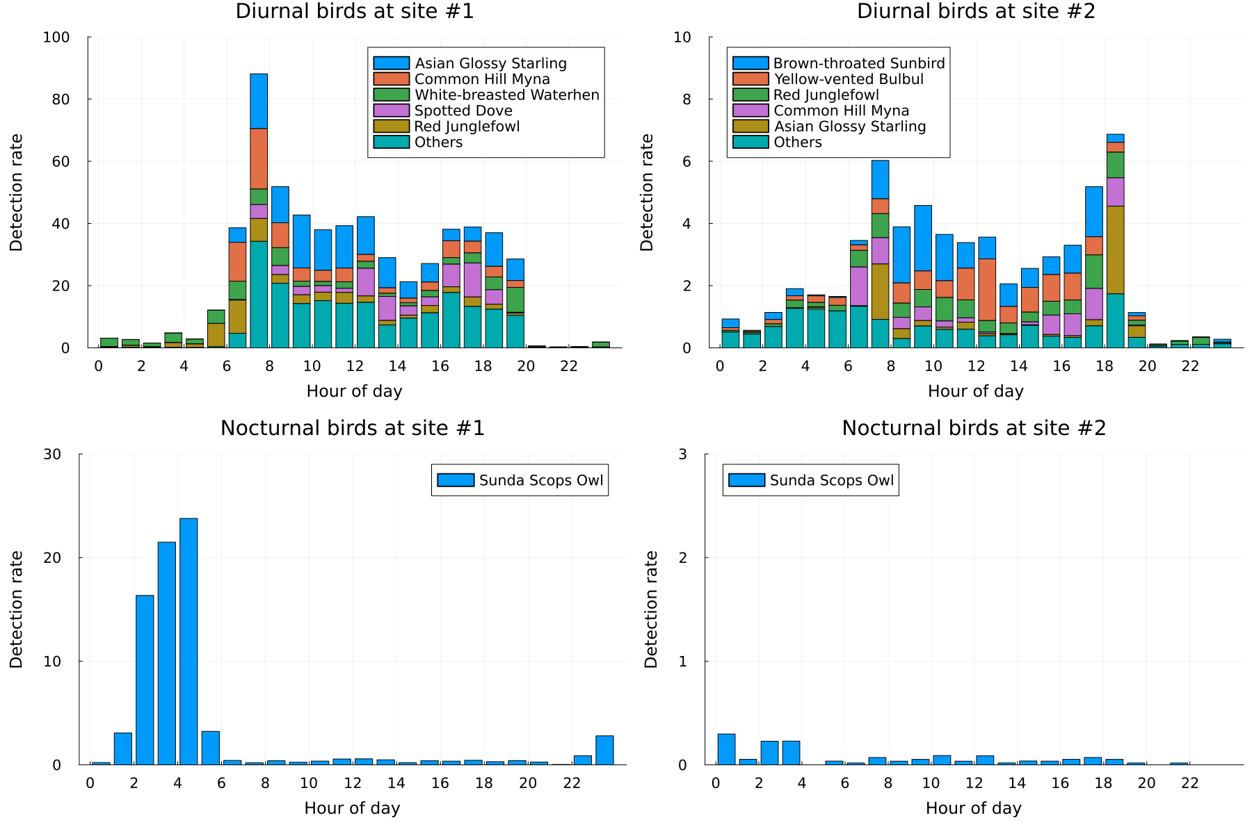
Figure 7: Mean detections by hour of day for dirunal birds (top row) and nocturnal birds (bottom row) over 10 days of recordings at each site. The top 5 species with highest detection count at each site are listed by name. Note that the y-axis differs between the plots.

Although the classifier has never seen the exact TFRs in the test set before, they all derive from classes which the model is trained to separate. Deploying the detector out in the field, on the other hand, exposes the classifier to a greater variety of sounds, many of which may be easily confused with some of the trained classes. In this part, we assess the model performance on raw, continuous streams of data, aiming to resemble a typical long-term monitoring situation. We first manually evaluate the model on a single day of soundscape recordings to shortlist classes with a reasonable level of precision. For practical reasons, we estimate class precision but not recall. That is, we verify the number of correct detections but do not attempt to estimate the number of missed detections as it would require very detailed, manual annotations of tens of hours of raw recordings. The shortlisted classes are then analyzed on 10 full days of recordings at both SBG sites to further evaluate the classifier but at an aggregated level without manual verification of each detection.

We randomly select a day in July 2020 from site #1 for the manual precision test and run the trained classifier on all 144 microphone-hours of recordings from that day (24 hours $\times$ 6 microphones). This yields about 250,000 TFRs prior to filtering. We disregard TFRs that either 1) do not pass the binary bird-pass filter (threshold = 0.5), 2) have a confidence score below 0.7, or 3) are assigned to the sink class. Additionally, we leave out 68 classes from species that are either known not to be present in the SBG or that are migratory and consequently not present in July. However, we do not ignore classes with low performance on the test set, as low test set performance may be a consequence of the misalignment between training and test samples mentioned earlier (Subsection 3.1), and not necessarily an indicator of poor model performance.

Among the remaining classes, we focus on those with distinct call characteristics for more reliable verifications. Up to 50 detected TFRs per class are randomly selected for manual verification. We keep classes with a minimum precision of 0.5, yielding 27 classes across 16 species (Table 3). Since the model is trained at TFR level rather than at species level, some species appear in several classes. A few classes achieve very high precision but based on very few detections. The “training samples” column lists the number of training samples before augmentation and suggests no strong correlation between precision and the number of training samples. The 9 classes with only 6 or fewer samples have a mean precision of 0.75 while the remaining 18 classes have a mean precision of 0.80.

For the aggregated evaluation, we run the detector on 10 randomly selected days between July and September 2020 for site #1 and 10 days between October 2020 and January 2021 for site #2. With 6 microphones recording in parallel (and occasional downtime), this translates to approximately 1350 microphone-hours of recordings for each site. For each class and hour of day, the detection rate is calculated as total detections divided by total hours of microphone recordings for that hour over the 10-day period. Located only $1.3^{\circ}$ north of Equator, Singapore experiences minimal changes in the timings of dawn and dusk over the year, with sunrise and sunset around 7 am and 7 pm every day. Detections are therefore naturally aligned with dawn and dusk without additional correction, despite spanning several months in time (Figure 7).

At site #1, the diurnal birds become vocally active around dawn with a distinct peak between 7 and 8 am. The activity then drops but stays quite high until it reaches a low-point between 2 pm and 3 pm. The activity rebounds in the late afternoon and stays high during dusk. There are very few detections of diurnal birds after 8 pm, until the Red Junglefowl (Gallus gallus, 176086) becomes active in the early morning between 5 and 6 am. The only nocturnal bird among the shortlisted ones, the Sunda Scops Owl (Otus lempiji, 1063234), is virtually absent during daytime and in the early evening until 10 pm. The majority of its detections occur from 2 am with a peak around 4–5 am, before detections plummet prior to the diurnal morning chorus.

Site #2 experiences a similar morning chorus peak as site #1 but a more distinct evening peak between 6 and 7 pm – largely attributed to the Asian Glossy Starling (Aplonis panayensis, 558724). This site also experiences few detections from diurnal birds after dusk but relatively many between midnight and dawn. Apart from the overall daily patterns, site #1 experiences about ten times higher detection rates compared to site #2.

Class	Training samples	Common name	Scientific name	TSN	Dete- ctions	True positives	Prec- ision
1	33	Asian Glossy Starling	Aplonis panayensis	558724	50	44	0.88
2	6	Black-naped Oriole	Oriolus chinensis	561694	14	10	0.71
3	4	Blue-eared Kingfisher	Alcedo meninting	554552	50	30	0.60
4	34	Brown-throated Sunbird	Anthreptes malacensis	558621	36	34	0.94
5	4	Brown-throated Sunbird	Anthreptes malacensis	558621	50	41	0.82
6	3	Changeable Hawk-eagle	Nisaetus cirrhatus	824093	2	2	1.00
7	50	Common Hill Myna	Gracula religiosa	179652	50	42	0.84
8	6	Common Hill Myna	Gracula religiosa	179652	24	22	0.92
9	3	Common Hill Myna	Gracula religiosa	179652	1	1	1.00
10	6	Crimson Sunbird	Aethopyga siparaja	558466	10	7	0.70
11	1	Greater Racket-tailed Drongo	Dicrurus paradiseus	559773	14	7	0.50
12	11	Olive-backed Sunbird	Cinnyris jugularis	916461	34	33	0.97
13	15	Olive-backed Sunbird	Cinnyris jugularis	916461	20	15	0.75
14	50	Olive-winged Bulbul	Pycnonotus plumosus	562623	50	40	0.80
15	22	Olive-winged Bulbul	Pycnonotus plumosus	562623	32	25	0.78
16	30	Olive-winged Bulbul	Pycnonotus plumosus	562623	50	26	0.52
17	33	Olive-winged Bulbul	Pycnonotus plumosus	562623	50	42	0.84
18	6	Red-whiskered Bulbul	Pycnonotus jocosus	178507	50	25	0.50
19	33	Red Junglefowl	Gallus gallus	176086	50	44	0.88
20	26	Red Junglefowl	Gallus gallus	176086	50	33	0.66
21	50	Red Junglefowl	Gallus gallus	176086	6	5	0.83
22	50	Spotted Dove	Spilopelia chinensis	1125210	50	48	0.96
23	50	Sunda Scops Owl	Otus lempiji	1063234	50	37	0.74
24	18	White-breasted Waterhen	Amaurornis phoenicurus	176385	15	12	0.80
25	11	White-breasted Waterhen	Amaurornis phoenicurus	176385	50	28	0.56
26	26	Yellow-vented Bulbul	Pycnonotus goiavier	562613	50	36	0.72
27	11	Yellow-vented Bulbul	Pycnonotus goiavier	562613	50	43	0.86

Table 3: Performance of shortlisted classes from a full day of continuous soundscape recordings at site #1. Bird names follow the Checklist of Bird Species for Singapore available at www.nparks.gov.sg/biodiversity/wildlife-in-singapore/species-list/birds. Taxonomic Serial Numbers (TSNs) are obtained from itis.gov.

4 Discussion

Several classes from the single-day performance test at site #1 achieve high precision despite very few training samples (Table 3). This result is encouraging, as it may allow researchers to train bioacoustic classifiers with very little labeled data. This is particularly valuable for monitoring initiatives of endangered or rare species as the low presence of such species makes it inherently hard to acquire acoustic samples for training. The performance gain over BirdNET on 103 bird species further suggests that the proposed methodology may not only be valuable for detecting rare species but may even enhance current state-of-the-art models for more common species, where large labeled datasets already exist.

The aggregated results from the 10-day test at each site add support to the manually verified precision test. The temporal detection patterns show a diurnal morning and evening chorus, few nighttime detections of diurnal birds, and few daytime detections of nocturnal birds, which align well with overall expected behavior. However, the relatively high detection rate between midnight and dawn of diurnal birds at site #2, suggests a lower model performance at this site. Most of these detections are classified as White-breasted Waterhen (Amaurornis phoenicurus, 176385) and inspection of some of these suggests that these are false positives originating from low-frequency sounds of cars passing by on a nearby road. This road is close enough to be heard at site #2 during the night, but likely too far to be detected at site #1. Lower model performance at site #2 may be a natural consequence of selection bias, as the evaluated classes are selected based on their precision at site #1. Nevertheless, this underscores the importance of enhancing classifier robustness to better generalize to new soundscapes, as even nearby survey sites can exhibit significant acoustic variability.

Site #2, apart from having more false positives during nighttime, also experiences about one-tenth the detection rate of site #1. This difference is likely not linked to variation in model performance between the sites but rather a result of differences in sound propagation. The recorders at site #1 were positioned around a lake with minimal obstruction between microphones, potentially allowing the same call to be detected on all 6 microphones simultaneously. In contrast, the recorders at site #2 were situated in an area with dense vegetation without direct line-of-sight between microphones. From calibration tests at site #2 using impulsive, high-SNR sounds, we found that the sounds were mostly audible on a single microphone at a time. Site #1, besides the multiplying effect present there, may further benefit from a longer detection range for each individual microphone.

5 Challenges and suggestions for future work

The soundscape in SBG is complex, comprising vocalizations not only from birds but also from amphibians, insects, reptiles, certain mammals like bats and squirrels, as well as anthropogenic sounds. The richness of this soundscape makes sound classification in long-duration recordings challenging as sounds from different sources may have high TFR-similarity. As a result, many of the classes that perform well on the test set (Subsection 3.1) experience low precision in raw soundscape recordings. We propose three possible remedies to address this challenge.

5.1 More data

The self-supervised component of the proposed method facilitates higher performance with less labeled training data. Nonetheless, additional training data would still be advantageous, as it would help mitigate confusion with similar sounds and enhance generalization capabilities. A pragmatic solution to handle false positives is to encourage the classifier to learn their features by continue to incorporate them into the training set, either to the sink class or to new or existing bird classes.

5.2 Higher resolution

Various bird species have demonstrated the ability to distinguish fine temporal variations in sound beyond the level of the human auditory system [34], and other studies emphasize the importance of incorporating high temporal features for acoustic bird classification [35]. For calls with very high temporal variability, the distinguishing features may be obscured or lost in the data compression stages. Retaining more of the information in the raw recording may help improve the performance for such classes. Three alternatives are to:

1. Increase the TFR resolution by reducing the max-pooling in the TFR extraction process.

2. Increase the resolution of the compressed TFR, either by reducing the convolutional filter sizes in the auto-encoder, or by increasing the latent space dimension.

3. Encourage the auto-encoder to pay more attention to vocalizations with high temporal variation, e.g., by oversampling such TFRs during training.

5.3 Acoustic-temporal context

Because the TFR extraction process is designed to separate disconnected regions of high energy in the input spectrogram, some TFRs will inevitably capture only part of the full call or song. In some cases, a small part of a call is sufficiently characteristic to distinguish it from other calls. In other cases, e.g. for many Sunbird species with very specific sequences of transient up- and downsweeps, it is hard to identify the exact species from a single up- or downsweep without also knowing what immediately preceded and followed. The dilation hyper-parameter in the spectrogram segmentation process (step 5 in Subsection 2.2) can be increased to merge TFRs that are spatially close in the time-frequency space but at the cost of introducing more extraneous signals into the TFRs. A better approach would involve keeping TFRs separated but still incorporate temporal context. One solution could be to train a classifier with not only the target TFR as input, but also with TFRs from the temporal vicinity of the target.

6 Conclusions

Protection of biodiversity is a major global concern. For conservation efforts to be effective and to track the effect of such initiatives, one need to monitor target habitats, often over long periods of time. Training machine learning models on bioacoustic data to monitor vocally active species is becoming increasingly common, but many methods rely on extensive annotated datasets for training. When developing bioacoustic monitoring systems in new regions, or when targeting rare or endangered species, annotated training data may be limited or unavailable and is often expensive to acquire – thereby increasing the barrier to perform studies. Methods that require less annotated data, and tools that can reduce the time and effort needed to obtain relevant training data, are therefore valuable. This is particularly true for birds, as the large number of species and their vast acoustic repertoire benefit from systems that can scale sustainably to new classes, and also because data annotation of bird sounds requires highly specialized expertise.

We propose a semi-supervised acoustic classification method that allows classification of sounds with limited annotated training data, and we evaluate it on bird recordings from Singapore. The embedding part of the network can accelerate the discovery and annotation of new classes by clustering embedding vectors from raw recordings. Its self-supervised nature, in combination with the pre-processing step that isolates individual bird calls, allows classification with fewer labeled training samples. We show that high classification precision can be achieved with very few labeled training samples, both on a controlled test set and in continuous soundscape recordings. Moreover, the proposed model outperforms the state-of-the-art BirdNET classifier on a test set covering 103 bird species, despite far less labeled training data. However, the rich soundscape in the SBG, with around 40,000 daily TFRs per microphone, makes it challenging to reject false positives. We thus propose various approaches to address this.

Although we validate the methods in this work on bird data, they are by no means restricted to bird vocalizations but can be applied to a wide range of acoustic tasks that involve clustering or classification of frequency-modulated sounds.

Declaration of Competing Interest

None.

References

- [1] C. J. Bibby, N. D. Burgess, D. A. Hill, Bird census techniques, revised Edition, Academic Press, London, UK, 2000.
- [2] W. Robinson, J. Brawn, S. Robinson, Forest bird community structure in central panama: Influence of spatial scale and biogeography, Ecological Monographs 70 (2000) 209–235. doi:https://doi.org/10.1890/0012-9615(2000)070[0209:FBCSIC]2.0.CO;2.
- [3] W. D. Robinson, A. C. Lees, J. G. Blake, Surveying tropical birds is much harder than you think: a primer of best practices, Biotropica 50 (6) (2018) 846–849. doi:https://doi.org/10.1111/btp.12608.
-
[4]
K. Darras, B. Furnas, I. Fitriawan, Y. Mulyani, T. Tscharntke, Estimating bird detection distances in sound recordings for standardizing detection ranges and distance sampling, Methods in Ecology and Evolution 9 (2018) 1928–1938.
URL https://doi.org/10.1111/2041-210X.13031 -
[5]
K. Darras, P. Batáry, B. J. Furnas, I. Grass, Y. A. Mulyani, T. Tscharntke, Autonomous sound recording outperforms human observation for sampling birds: a systematic map and user guide, Ecological Applications 29 (6) (2019) e01954.
URL https://esajournals.onlinelibrary.wiley.com/doi/abs/10.1002/eap.1954 - [6] A. Wheeldon, H. L. Mossman, M. J. P. Sullivan, J. Mathenge, S. R. de Kort, Comparison of acoustic and traditional point count methods to assess bird diversity and composition in the aberdare national park, kenya, African Journal of Ecology 57 (2) (2019) 168–176. doi:https://doi.org/10.1111/aje.12596.
- [7] S. Hoefer, D. McKnight, S. Allen-Ankins, E. Nordberg, L. Schwarzkopf, Passive acoustic monitoring in terrestrial vertebrates: a review, Bioacoustics 32 (2023) 506–531. doi:10.1080/09524622.2023.2209052.
- [8] A. Hingston, T. Wardlaw, S. Baker, G. Jordan, Data obtained from acoustic recording units and from field observer point counts of tasmanian forest birds are similar but not the same, Australian Field Ornithology 35 (2018) 30–39. doi:10.20938/afo35030039.
- [9] D. Stowell, Computational bioacoustics with deep learning: a review and roadmap, PeerJ 10 (2022) e13152.
-
[10]
S. Kahl, C. M. Wood, M. Eibl, H. Klinck, Birdnet: A deep learning solution for avian diversity monitoring, Ecological Informatics 61 (2021) 101236.
doi:https://doi.org/10.1016/j.ecoinf.2021.101236.
URL https://www.sciencedirect.com/science/article/pii/S1574954121000273 - [11] J. Deng, W. Dong, R. Socher, L.-J. Li, K. Li, L. Fei-Fei, Imagenet: A large-scale hierarchical image database, in: 2009 IEEE Conference on Computer Vision and Pattern Recognition, 2009, pp. 248–255. doi:10.1109/CVPR.2009.5206848.
- [12] J. F. Gemmeke, D. P. W. Ellis, D. Freedman, A. Jansen, W. Lawrence, R. C. Moore, M. Plakal, M. Ritter, Audio set: An ontology and human-labeled dataset for audio events, in: 2017 IEEE International Conference on Acoustics, Speech and Signal Processing (ICASSP), 2017, pp. 776–780. doi:10.1109/ICASSP.2017.7952261.
-
[13]
J. LeBien, M. Zhong, M. Campos-Cerqueira, J. P. Velev, R. Dodhia, J. L. Ferres, T. M. Aide, A pipeline for identification of bird and frog species in tropical soundscape recordings using a convolutional neural network, Ecological Informatics 59 (2020).
doi:https://doi.org/10.1016/j.ecoinf.2020.101113.
URL https://www.sciencedirect.com/science/article/pii/S1574954120300637 -
[14]
A. R. Rodrigo Manriquez P, Sonja A. Kotz, B. de Boer, Bioacoustic classification of a small dataset of mammalian vocalisations using deep learning, Bioacoustics 33 (4) (2024) 354–371.
doi:10.1080/09524622.2024.2354468.
URL https://doi.org/10.1080/09524622.2024.2354468 -
[15]
E. Tsalera, A. Papadakis, M. Samarakou, Comparison of pre-trained cnns for audio classification using transfer learning, Journal of Sensor and Actuator Networks 10 (4) (2021).
doi:10.3390/jsan10040072.
URL https://www.mdpi.com/2224-2708/10/4/72 -
[16]
I. Nolasco, S. Singh, V. Morfi, V. Lostanlen, A. Strandburg-Peshkin, E. Vidaña-Vila, L. Gill, H. Pamuła, H. Whitehead, I. Kiskin, F. H. Jensen, J. Morford, M. G. Emmerson, E. Versace, E. Grout, H. Liu, B. Ghani, D. Stowell, Learning to detect an animal sound from five examples, Ecological Informatics 77 (2023).
doi:https://doi.org/10.1016/j.ecoinf.2023.102258.
URL https://www.sciencedirect.com/science/article/pii/S157495412300287X - [17] F. Briggs, B. Lakshminarayanan, L. Neal, X. Fern, R. Raich, S. Frey, A. Hadley, M. Betts, Acoustic classification of multiple simultaneous bird species: A multi-instance multi-label approach, The Journal of the Acoustical Society of America 131 (2012) 4640–50. doi:10.1121/1.4707424.
-
[18]
C. Wood, S. Kahl, S. Barnes, R. Horne, C. Brown, Passive acoustic surveys and the birdnet algorithm reveal detailed spatiotemporal variation in the vocal activity of two anurans, Bioacoustics 32 (5) (2023) 532–543.
doi:10.1080/09524622.2023.2211544.
URL https://doi.org/10.1080/09524622.2023.2211544 - [19] M. Lasseck, Audio-based bird species identification with deep convolutional neural networks, 2018.
- [20] G. Gupta, M. Kshirsagar, M. Zhong, S. Gholami, J. Lavista Ferres, Comparing recurrent convolutional neural networks for large scale bird species classification, Scientific Reports 11 (2021). doi:10.1038/s41598-021-96446-w.
-
[21]
A. Thakur, D. Thapar, P. Rajan, A. Nigam, Deep metric learning for bioacoustic classification: Overcoming training data scarcity using dynamic triplet loss, The Journal of the Acoustical Society of America 146 (1) (2019) 534–547.
doi:10.1121/1.5118245.
URL https://doi.org/10.1121/1.5118245 -
[22]
A. Noumida, R. Rajan, Multi-label bird species classification from audio recordings using attention framework, Applied Acoustics 197 (2022).
doi:https://doi.org/10.1016/j.apacoust.2022.108901.
URL https://www.sciencedirect.com/science/article/pii/S0003682X22002754 - [23] S. Hexeberg, H. Vishnu, K. T. Beng, A. Ho, W. Yusong, M. Chitre, K. Tun, K. Lim, Acoustic detector for multiple vocalizing marine mammal individuals, in: OCEANS 2023 - Limerick, 2023, pp. 1–8. doi:10.1109/OCEANSLimerick52467.2023.10244432.
- [24] A. J. Fairbrass, P. Rennert, C. Williams, H. Titheridge, K. E. Jones, Biases of acoustic indices measuring biodiversity in urban areas, Ecological Indicators 83 (2017) 169–177. doi:https://doi.org/10.1016/j.ecolind.2017.07.064.
- [25] R. Gibb, E. Browning, P. Glover-Kapfer, K. E. Jones, Emerging opportunities and challenges for passive acoustics in ecological assessment and monitoring, Methods in Ecology and Evolution 10 (2) (2019) 169–185. doi:https://doi.org/10.1111/2041-210X.13101.
- [26] A. Hughes, M. Orr, F. Lei, Q. Yang, H. Qiao, Understanding drivers of global urban bird diversity, Global Environmental Change 76 (2022). doi:10.1016/j.gloenvcha.2022.102588.
- [27] J. Wong, M. Soh, B. W. Low, K. Er, Tropical bird communities benefit from regular-shaped and naturalised urban green spaces with water bodies, Landscape and Urban Planning 231 (2023). doi:10.1016/j.landurbplan.2022.104644.
- [28] L. Sutherland, G. Daigle, Atmospheric Sound Propagation, J. Wiley, 1998, pp. 341–365.
- [29] D. Kingma, J. Ba, Adam: A method for stochastic optimization, in: International Conference on Learning Representations (ICLR), 2015.
- [30] T. Chen, S. Kornblith, M. Norouzi, G. Hinton, A simple framework for contrastive learning of visual representations, arXiv preprint arXiv:2002.05709 (2020).
- [31] J. Salamon, C. Jacoby, J. P. Bello, A dataset and taxonomy for urban sound research, in: 22nd ACM International Conference on Multimedia (ACM-MM’14), Orlando, FL, USA, 2014, pp. 1041–1044.
- [32] S. Kahl, Birdnet-analyzer, https://github.com/kahst/BirdNET-Analyzer, accessed: 2024-10-27.
- [33] S. Taubert, birdnet, https://pypi.org/project/birdnet/, accessed: 2024-10-27.
- [34] R. J. Dooling, M. R. Leek, O. Gleich, M. L. Dent, Auditory temporal resolution in birds: Discrimination of harmonic complexes, The Journal of the Acoustical Society of America 112 (2) (2002) 748–759. doi:10.1121/1.1494447.
- [35] D. Stowell, M. D. Plumbley, Large-scale analysis of frequency modulation in birdsong data bases, Methods in Ecology and Evolution 5 (9) (2014) 901–912. doi:https://doi.org/10.1111/2041-210X.12223.