Violation of non-Abelian Bianchi identity and QCD topology
-An Abelian mechanism without instantons-

Abstract

The violation of non-Abelian Bianchi identity (VNABI) $J_{\mu}(x)$ if it exists is equal to 8 Abelian magnetic monopole currents $k^{a}_{\mu}(x)\ \ (a=1\sim 8)$. Abelian monopoles can exist without any artificial Abelian projection. When $J_{\mu}$ condenses in the vacuum, color confinement of QCD is realized by the Abelian dual Meissner effect. Moreover VNABI affects topological features of QCD drastically. Firstly, self-dual instantons can not be a classical solution of QCD. Secondly, the topological charge density $\rho_{t}(x)=\text{Tr}G_{\mu\nu}(x)G^{*}_{\mu\nu}(x)$ is not expressed by a total derivative of the Chern-Simons density $K_{\mu}(x)=(g^{2}/8\pi^{2})\epsilon_{\mu\nu\rho\sigma}\text{Tr}(A_{\nu}(\partial_{\rho}A_{\sigma}-i2gA_{\rho}A_{\sigma}/3))$, but has an additional term $L(x)=2\text{Tr}(J_{\mu}(x)A_{\mu}(x))$, that is, $\partial_{\mu}K_{\mu}(x)=(g^{2}/16\pi^{2})(\rho_{t}(x)-L(x))$. Thirdly, the axial $U(1)$ anomaly is similarly modified as $\partial_{\mu}j_{\mu}^{5}(x)=2m\bar{\psi}(x)\gamma_{5}\psi(x)+(g^{2}/8\pi^{2})(\rho_{t}(x)-L(x))$ while the Atiyah-Singer index theorem is unchanged. These facts suggest that an Abelian mechanism based on the Abelian monopoles responsible for color confinement play an important role also in these topological quantities in place of instantons. The integrated additional term $\chi=(g^{2}/16\pi^{2})\int d^{4}xL(x)$ is evaluated in the framework of Monte-Carlo simulations on small $24^{4}$ lattices adopting an improved $SU(2)$ gluon action with the help of smoothing methods such as the Maximal Center gauge (MCG), the Maximal Abelian gauge plus subsequent $U(1)$ gauge (MAU1) and the gradient flow with DBW2 flow action. The term $\chi$ tends to vanish after small gradient flow time ($\tau$) when infrared monopoles responsible for color confinement are also much suppressed. The bosonic definition of the topological charge $Q_{t}$ and its Abelian counterpart $Q_{a}\equiv(g^{2}/16\pi^{2})\int d^{4}x\text{Tr}(f_{\mu\nu}f_{\mu\nu}^{*})$ written by Abelian field strengths are measured also on the lattices. When $\chi$ is zero, $Q_{a}$=3$Q_{t}$ is expected theoretically, but $Q_{a}$ defined by a simple Abelian plaquette is fluctuating between -2 and -3 in MCG and around -2 in MAU1 when $Q_{t}$ is amost stabilized around -1 after $\tau$ is larger than 2. The MAU1 data of $Q_{a}(A)$ and $\chi$ become totally random rapidly when $\tau$ is larger than 20.

I Introducation

In non-perturbative QCD, color confinement and chiral symmetry breaking are two important unsolved problems. Topological objects such as monopoles and instantons are believed to play an important role in these phenomena. The relation between these topological quantities has been unclear. The aim of this work is to show an interesting possibility that an Abelian mechansim based on Abelian magnetic monopoles responsible for color confinement play an important role also in anomalous chiral $U(1)$ breaking and the vacuum transition between degenerate vacua in place of instantons.

As a theoretical background of numerical results showing perfect Abelian and monopole dominances without any artificial Abelian projectionSuzuki:2008 ; Suzuki:2009 , the present authorSuzuki:2014wya ; Suzuki:2017 proposed a new idea of Abelian monopoles in QCD due to violation of non-Abelian Bianchi identity Bonati:2010tz without any Abelian projectiontHooft:1981ht . When gauge fields in QCD contain a line singularity of the Dirac typeDirac:1931 , the non-Abelian Bianchi identity is violated. The violation of the non-Abelian Bianchi identity (VNABI) $J_{\mu}(x)$ is equivalent to 8 Abelian magnetic monopole currents $k^{a}_{\mu}(x)\ \ (a=1\sim 8)$ defined by violation of the Abelian Bianchi identities in $SU(3)$. When $J_{\mu}$ condenses in the vacuum, color confinement of QCD is realized by the Abelian dual Meissner effectNambu:1974 ; Mandelstam:1974pi ; tHooft:1975pu .

Table 1: Non-Abelian (NA), Abelian (A) and monopole (M) string tensions from $SU(2)$ static potentials at $T=0.8T_{c}$, where $T_{c}$ is the critical temperature. The data are taken from Ref.Suzuki:2009 .

Lattice	$\beta$	$a(\beta)$fm	$\sigma_{NA}a^{2}$	$\sigma_{A}a^{2}$	$\sigma_{M}a^{2}$
$24^{3}\times 4$	$2.20$	$0.211(7)$	$0.181(8)$	$0.183(8)$	$0.183(6)$
$24^{3}\times 6$	$2.35$	$0.137(9)$	$0.072(3)$	$0.073(4)$	$0.073(4)$
$36^{3}\times 6$	$2.35$	$0.137(9)$	$0.072(3)$	$0.073(2)$	$0.073(3)$
$36^{3}\times 6$	$2.43$	$0.1029(4)$	$0.0415(9)$	$0.041(2)$	$0.043(3)$

1)The color electric flux between a static quark and antiquark is squeezed which leads us to a linear potential with the string tension $\sigma$Wilson:1974 . If the flux squeezing is owing to a solenoidal Abelian monopole current as suggested by ADME, the string tension is explained by those of Abelian and monopole static potentials, i.e., $\sigma=\sigma_{a}=\sigma_{m}$. This is called as Abelian and monopole dominances. They are seen numerically firstSuzuki:1990 in maximal Abelian gauge (MAG)Kronfeld:1987ri ; Kronfeld:1987vd and later in other gauges and even without any gauge-fixingShiba:1994 ; Stack:1994 ; Koma:2003B ; Sekido:2007 ; Suzuki:2008 ; Suzuki:2009 ; Sakumichi:2014 ; Ishiguro:2022 ; Suzuki:2023 . See for example Table 1 cited from Suzuki:2009 .

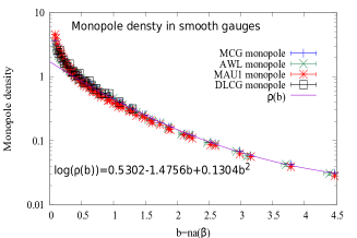
Figure 1: Abelian monopole densities versus $b=na(\beta)$ in various gauges. This figure is cited from Suzuki:2017 .

2) The renormalization-group (RG) studyWilson:1974B utilizing a block-spin transformation is a powerful method to study the continuum limit in the framework of lattice field theories like a $\phi^{4}$ theoryAizenman:1982 ; Frohlich:1982 . The block-spin RG study is also very powerful to study the continuum limit of the monopole dynamics described by integer Abelian lattice monopole variablesShiba:1994db . It is possible to prove existence of the continuum limit of the monopole density and infrared effective monopole action in $SU(2)$Shiba:1994db ; Suzuki:2017 ; Suzuki:2017zdh and in $SU(3)$Sakumichi:2014 ; Suzuki:2023 ; Suzuki:2024 . As an example, see the data of the $SU(2)$ monopole density $\rho(a(\beta),n)$ in Fig.1 cited from Suzuki:2017 . $\rho(a(\beta),n)$ is a function of $b=na(\beta)$ alone for $3.0\leq\beta\leq 3.9$ and $n=1,2,3,4,6,8,12$ step blockings. A scaling is seen as well as gauge choice independence. When we take $n\to\infty$ for fixed $b=na(\beta)$, then $a(\beta)\to 0$, i.e., the continuum limit. Beautiful scaling behaviors suggesting the existence of the continuum limit are observed.

Here we report very interesting new facts concerning VNABI in addition to the above color confinement mechansim. Namely VNABI if it exists modifies drastically QCD topology such as chiral $U(1)$ anomaly and the vacuum transition.

II VNABI and topology in QCD

II.1 VNABI

Why VNABI is equivalent to Abelian magnetic monopole currents is discussed in Suzuki:2014wya ; Suzuki:2017 . Consider $SU(2)$ QCD for simplicity. Define a covariant derivative operator $D_{\mu}=\partial_{\mu}+igA_{\mu}(x)$ where $A_{\mu}(x)=A_{\mu}^{a}\sigma_{a}/2$. The Jacobi identities are expressed as $\epsilon_{\mu\nu\rho\sigma}[D_{\nu},[D_{\rho},D_{\sigma}]]=0$. By direct calculations, one gets $[D_{\rho},D_{\sigma}]=-igG_{\rho\sigma}+[\partial_{\rho},\partial_{\sigma}]$, where the second commutator term of the partial derivative operators can not be discarded in general, since gauge fields may contain a line singularity. Actually, it is the origin of the violation of the non-Abelian Bianchi identities (VNABI) as shown in the following. The relation $[D_{\nu},G_{\rho\sigma}]=D_{\nu}G_{\rho\sigma}$ and the Jacobi identities lead us to

$$J_{\mu} \equiv D_{\nu}G^{*}_{\mu\nu}=\frac{1}{2}\epsilon_{\mu\nu\rho\sigma}[\partial_{\rho},\partial_{\sigma}]A_{\nu}=\partial_{\nu}f^{*}_{\mu\nu}\equiv k_{\mu},$$ (1)

where $f_{\mu\nu}$ is defined as $f_{\mu\nu}=\partial_{\mu}A_{\nu}-\partial_{\nu}A_{\mu}$. Eq.(1) shows that the violation of the non-Abelian Bianchi identities (VNABI) is equivalent to that of the Abelian Bianchi identities. Eq.(1) is gauge covariant and therefore a non-zero $J_{\mu}$ is a gauge-invariant property. As shown in Suzuki:2014wya ; Suzuki:2017 , $J_{\mu}=k_{\mu}$ transforms as an adjoint operator and satisfies both $D_{\mu}J_{\mu}=0$ and $\partial_{\mu}J_{\mu}=0$ although it looks unlikely. The Dirac quantization conditionDirac:1931 is satisfied, i.e, $gg_{m}=4\pi n$ where $g_{m}$ is a magnetic charge and $n$ is an integer.

II.2 Instantons and VNABI

It is known that a classical solution of Euclidian QCD called instantonBelavin:1975 is important in the quantum transition between degenerate vacua with a different winding number. Instantons give us also an integer topological charge $Q_{t}$ defined later. The instanton is a solution satisfying the self-duality condition $G_{\mu\nu}=G^{*}_{\mu\nu}$. However when VNABI exists, it is easy to prove that there cannot exist such an instanton solution, since the self-duality condition leads us automatically to the non-Abelian Bianchi identity $D_{\mu}G^{*}_{\mu\nu}=0$ from the equation of motion of QCD, that is, $D_{\mu}G_{\mu\nu}=0$.

II.3 The topological charge

The topological charge $Q_{t}(A)$ and the topological charge density are defined Mueller-Preussker:2011 by

$$Q_{t}(A) = \frac{g^{2}}{16\pi^{2}}\int d^{4}x\rho_{t}(x),$$ (2)

$$\rho_{t}(x) \equiv \text{Tr}(G_{\mu\nu}G^{*}_{\mu\nu})$$ (3)

and gauge-variant Chern-Simons density is written as

$$K_{\mu}(x)$$

$$= \frac{g^{2}}{8\pi^{2}}\epsilon_{\mu\nu\rho\sigma}\text{Tr}\left[A_{\nu}(x)(\partial_{\rho}A_{\sigma}(x)-\frac{2ig}{3}A_{\rho}(x)A_{\sigma}(x))\right].$$

Evaluate the divergence $\partial_{\mu}K_{\mu}(x)$:

$$\partial_{\mu}K_{\mu}(x) = \frac{g^{2}}{16\pi^{2}}[\rho_{t}(x)-L(x)],$$ (4)

where $L(x)\equiv 2\text{Tr}(A_{\mu}(x)J_{\mu}(x))$. $L(x)$ is zero if gauge fields are regular as usually assumed. But when VNABI exists, it is non-vanishing. The term $L(x)$ is gauge variant. But we can prove that $\int d^{4}xL(x)$ is gauge invariant, since $V(x)L(x)V^{{\dagger}}(x)-L(x)=2\partial_{\mu}(V_{0}(x)\vec{V}(x)\cdot\vec{k}_{\mu}(x))/g$, where $V(x)=V_{0}(x)+i\vec{V}(x)\cdot\vec{\sigma}$ is a gauge transformation matrix. The action becomes vanishing at the boundary, so that gauge fields become a pure gauge $(i/g)U^{{\dagger}}(x)\partial_{\mu}U(x)$ with a regular $U(x)$. Hence we get $|\vec{k}(x)|\to 0$ for $|x|\to\infty$. Namely $\int d^{4}x\Delta L(x)=0$.

II.4 A vacuum-to-vacuum amplitude

Let us compute a vacuum-to-vacuum amplitude:

$$Z = <vac|\exp(-\frac{1}{\hbar}\hat{H}(\tau-\tau_{0})|vac>.$$

The vacuum $A^{vac}_{\mu}(x)$ is characterized by integer winding number $\omega_{\infty}$ as follows:

$$\omega_{\infty} = \oint_{S^{3}(|x|\to\infty)}d\sigma_{\mu}K_{\mu}(x)=\oint d^{3}\sigma n_{\nu}K_{\nu}$$ (5)

$$= \frac{ig^{3}}{24\pi^{2}}\oint d^{3}\sigma n_{\nu}\epsilon_{\mu\nu\rho\sigma}\text{Tr}\left[A_{\nu}A_{\rho}A_{\sigma}\right],$$

where at the boundary $G_{\mu\nu}=0$ and then $\epsilon_{\mu\nu\rho\sigma}\partial_{\rho}A_{\sigma}=ig\epsilon_{\mu\nu\rho\sigma}A_{\rho}A_{\sigma}$. Thus

$$\omega_{\infty}=\frac{1}{24\pi^{2}}\oint d^{3}\sigma$$

$$\times n_{\nu}\epsilon_{\mu\nu\rho\sigma}\text{Tr}\left[(U^{{\dagger}}\partial_{\nu}U)(U^{{\dagger}}\partial_{\rho}U)(U^{{\dagger}}\partial_{\sigma}U)\right],$$

which is the winding number taking an integer. Hence we get

$$\omega_{\infty} = Q_{t}(A)-\chi$$ (6)

$$\chi \equiv \frac{g^{2}}{8\pi^{2}}\int d^{4}x\text{Tr}(J_{\mu}(x)A_{\mu}(x)).$$

Since $J_{\mu}(x)=\partial_{\nu}f^{*}_{\mu\nu}(x)$, it is possible to prove also

$$3\omega_{\infty} = Q_{a}(A)-\chi,$$ (7)

$$Q_{a}(A) \equiv \frac{g^{2}}{16\pi^{2}}\int d^{4}x\text{Tr}(f_{\mu\nu}f^{*}_{\mu\nu}),$$

where we use a partial integral and the above boundary condition again. To be noted that $Q_{t}(A)$ is equal to the integral over an inner product of non-Abelian electric and magnetic fields, whereas $Q_{a}(A)$ is that of Abelian electric and magnetic fields.

Consider a large gauge transformation $\hat{T}(U)$ such that $\hat{T}|n>=|n+1>$. Hamiltonian $\hat{H}$ is invariant under $\hat{T}(U)$: $[\hat{T},\hat{H}]=0$. Physical gauge invariant $\theta$-vacuum is defined as follows:

$$\hat{H}|\theta> = E_{0}|\theta>,$$

$$|\theta> \equiv \sum_{n=-\infty}^{n=\infty}e^{in\theta}|n>.$$

The vacuum transition amplitude is calculated as

$$Z=<\theta^{\prime}|\exp(-\hat{H}\tau)|\theta>$$

$$= \sum_{n^{\prime},n}e^{i(n\theta-n^{\prime}\theta^{\prime})}\int DA_{\mu}(x)|_{n,n^{\prime}}\exp(-S[A]).$$

$\int DA_{\mu}(x)|_{n,n^{\prime}}\exp(-S[A])$ depends on $\nu=n-n^{\prime}$. From Eq.(6), we see $n^{\prime}-n=Q_{t}(A)-\chi$ and

$$Z = \sum_{n}e^{in(\theta-\theta^{\prime})}\sum_{\nu}\int DA_{\mu}(x)|_{\nu}$$

$$\times \exp[-S[A]-i(Q_{t}(A)-\chi)\theta^{\prime}].$$

II.5 Chiral $U(1)$ anomaly and VNABI

Let us next discuss the chiral $U(1)$ anomaly. Here we follow the worksFujikawa:1979 ; Alvarez-Gaume:1984 . When we define $u_{i}(x)$ as the normalized zero-mode eigenvectors of the Dirac operator $\not{D}_{\mu}=(\partial_{\mu}+igA_{\mu})\gamma_{\mu}$ of which $n_{+}$ eigenvectors have positive chirality $\gamma_{5}u_{i}(x)=u_{i}(x)$ and $n_{-}$ have negative chirality $\gamma_{5}u_{i}(x)=-u_{i}(x)$. Then without VNABI, we get the Atiyah-Singer index theorem $n_{+}-n_{-}=\nu$, where $\nu$ denotes the Pontryagin index $\nu=-Q_{t}(A)$ in (3)Fujikawa:1979 . When VNABI exists, what happens about the Atiyah-Singer index theorem?

Consider the gauge invariant Lagrangian

$$L=\bar{\psi}(\not{D}+m)\psi+\frac{1}{2}TrG_{\mu\nu}G_{\mu\nu}$$

and perform a flavor singlet $\gamma_{5}$ transformation $\psi(x)\to\exp[i\alpha(x)\gamma_{5}]\psi(x)$. Then we get for infinitesimal $\alpha(x)$

$$L\to L-i\partial_{\mu}\alpha(x)\bar{\psi}\gamma_{\mu}\gamma_{5}\psi(x)-2im\alpha(x)\bar{\psi}\gamma_{5}\psi.$$

We also take into account the change of the measure of the functional integral, i.e., the Jacobian factor. Expand $\psi(x)$ and $\bar{\psi}(x)$ as $\psi(x)=\sum_{n}a_{n}\phi_{n}(x),\ \ \ \bar{\psi}(x)=\sum\phi_{n}^{{\dagger}}(x)\bar{b}_{n}$, in terms of a complete set of eigenfunctions of the Hermitian operator $\not{D}$: $\not{D}\phi_{n}(x)=\lambda_{n}\phi_{n}(x)$. For infinitesimal $\alpha(x)$, the Jacobian factor becomes

$$\exp\left(-2i\int d^{4}x\alpha(x)\sum_{n}\phi_{n}^{{\dagger}}(x)\gamma_{5}\phi_{n}(x)\right),$$

which is divergent and can be regularized with a Gaussian cut-off:

$$\sum_{n}\phi_{n}^{{\dagger}}(x)\gamma_{5}\phi_{n}(x)$$

$$\to \lim_{M\to\infty}\sum_{n}\phi_{n}^{{\dagger}}(x)\gamma_{5}\exp[-(\lambda_{n}/M)^{2}]\phi_{n}(x)$$

$$= \lim_{M\to\infty,y\to x}\text{Tr}\gamma_{5}\exp[-(\not{D}/M)^{2}]\delta(x-y).$$

Now

$$(\not{D})^{2} = D_{\mu}D_{\mu}+\frac{1}{4}\left([\partial_{\mu},\partial_{\nu}]+gG_{\mu\nu}\right)[\gamma_{\mu},\gamma_{\nu}].$$

When the gauge fields are regular, the term $[\partial_{\mu},\partial_{\nu}]$ is dropped. But when VNABI exists, it cannot be discarded. Actually

$$\text{Tr}\gamma_{5}e^{-(\not{D}/M)^{2}}\delta(x-y)$$

$$= e^{-\frac{D_{\mu}^{2}}{M^{2}}}\text{Tr}\gamma_{5}(\frac{1}{2!})(-\frac{1}{4M^{2}})^{2}[\gamma_{\mu},\gamma_{\nu}][\gamma_{\alpha},\gamma_{\beta}]$$

$$\times([\partial_{\mu},\partial_{\nu}]+gG_{\mu\nu})([\partial_{\alpha},\partial_{\beta}]+gG_{\alpha\beta})).$$

Then finally we get

$$\sum_{k}\phi_{k}^{{\dagger}}(x)\gamma_{5}\phi_{k}(x)$$ (8)

$$= -\frac{g^{2}}{16\pi^{2}}Tr(G^{*}_{\mu\nu}G_{\mu\nu})+\frac{g^{2}}{8\pi^{2}}\text{Tr}(J_{\mu}A_{\mu}).$$

The lefthand side of Eq.(8) vanishes for the eigenfunctions with eigenvalue $\lambda_{k}\neq 0$ since $\gamma_{5}\phi_{k}(x)$ has the eigenvalue $-\lambda_{k}$. Then LHS becomes

$$\int d^{4}x\left(\sum_{i=1}^{n_{+}}\phi^{*}_{i+}(x)\phi_{i+}(x)-\sum_{i=1}^{n_{-}}\phi^{*}_{i-}(x)\phi_{i-}(x)\right)$$

$$= n_{+}-n_{-}.$$

Hence we get

$$n_{+}-n_{-}=-Q_{t}+\chi$$ (9)

When we compare Eq.(9) with Eq.(6), we see

$$n_{-}-n_{+}=\omega_{\infty}.$$ (10)

The Atiyah-Singer index theorem is unchanged also under the existence of VNABI.

Eq.(9) and Eq.(6) say that the modifications due to VNABI appear always as a combination of $Q_{t}-\chi$. All previous discussions about the topological charge $Q_{t}$ are replaced by $Q_{t}-\chi$. Topological features concerning strong CP problemSchierholz:2024 ; Hook:2018 are also unchanged.

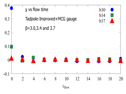
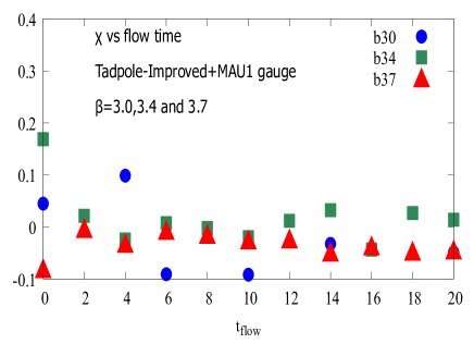
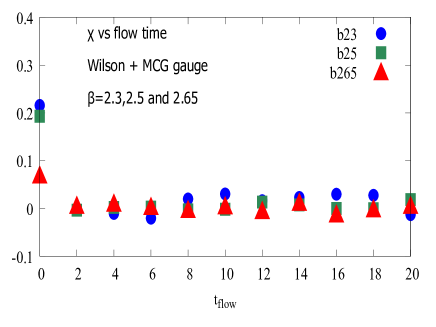
Figure 2: The additional term $\chi$ in the tadpole-improved action with MCG gauge (top), in tadpole-improved action with MAU1 gauge (middle) and in the Wilson action with MCG gauge (down).

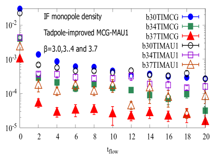
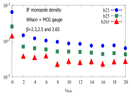
Figure 3: IF monopole density in the tadpole-improved action with MCG and MAU1 gauges(top) and in the Wilson action with MCG gauge (down) versus gradient flow time.

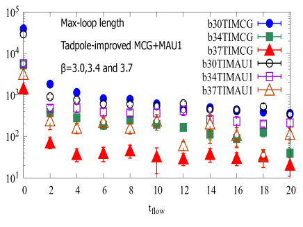
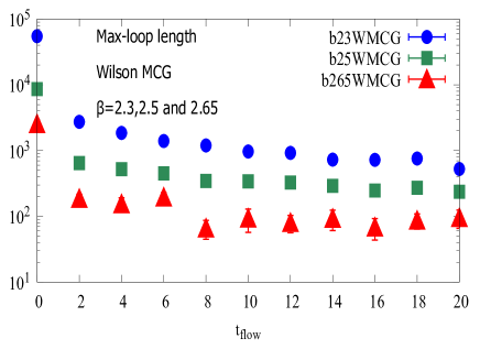
Figure 4: Maximum loop lengths in the tadpole-improved action with MCG and MAU1 gauges(top) and in the Wilson action with MCG gauge (down) versus gradient flow time.

Figure 5: The Non-Abelian Creutz ratio $\chi(4,4)$ versus gradient flow time in the tadpole-improved and the Wilson actions..

III Lattice numerical studies of VNABI and topology

Although naively lattice gauge fields are topologically trivial, the discussion of the topology on a lattice is meaningful sufficiently close to the continuum limitLuscher:1982 . On a lattice, gauge fields are described by a compact field $U(s.\mu)$ on a link $(s,\mu)$ where $s$ denotes a site and $\mu$ is a direction. As a lattice gauge action, we adopt the following:

$$S=\beta(c_{0}\sum_{pl}S_{pl}+c_{1}\sum_{rt}S_{rt}),$$ (11)

where $S_{pl}$ and $S_{rt}$ denote a $1\times 1$ plaquette and $1\times 2$ rectangular loop terms in the action. Here we adopt the tadpole-improved action where $c_{0}=1$ and $c_{1}=-1/(20u_{0})^{2}$ and $u_{0}$ is the $SU(2)$ tadpole improvement factorAlford:1995hw . The lattice size is $24^{4}$ and we consider $\beta=3.0\sim 3.7$. Only the data at three $\beta$ points: $a(3.0)=0.17279(19)$fm, $a(3.4)=0.08436(9)$fm and $a(3.7)=0.05252(23)$fm are plotted in some figures as typical $\beta$ points with respect to the tadpole improved case. For comparison, we also consider the usual Wilson action with $c_{0}=1\ \ c_{1}=0$ at $a(2.3)=0.16634(167)$fm, $a(2.5)=0.08598(146)$fm, $a(2.65)=0.0529(19)$fm.

III.1 Evaluation of the additional term $\chi$

Let us consider what happens about the additional term $\chi$ on the lattice. The term $\chi$ is written in terms of Abelian monopole currents. First of all, we have to extract a link field $\theta_{\mu}^{a}$ having a color $a$ out of $U(s,\mu)$. The following method is found to be applicable for Abelian confinement pictures both in $SU(2)$Suzuki:2008 and $SU(3)$Ishiguro:2022 in accord with the previous definition used in the old Abelian projection. We maximize the following quantity locally

$$R^{a}=\mathrm{Re}\mathop{\rm Tr}\left\{\exp(i\theta_{\mu}^{a}(s)\lambda^{a})U_{\mu}^{{\dagger}}(s)\right\},$$ (12)

where $\lambda^{a}$ is the Gell-Mann matrix and the sum over $a$ is not taken. In $SU(2)$, Eq.(12) leads us to

$$\theta_{\mu}^{a}(s)=\tan^{-1}\left\{\frac{U_{\mu}^{a}(s)}{U_{\mu}^{0}(s)}\right\},$$ (13)

where $U_{\mu}(s)=U_{\mu}^{0}(s)+i\sum_{a}\sigma^{a}U_{\mu}^{a}(s)$. In the calculation of $\chi$, we use a compact form $sin\theta_{\mu}^{a}(s)$ as a field corresponding to $A_{\mu}^{a}(x)$ in $\chi(x)$.

Next at present a reliable lattice monopole definition is the one proposed by DeGrand-ToussaintDeGrand:1980eq which counts the number of the Dirac string coming out of monopoles. A plaquette variable $\theta_{\mu\nu}^{a}(s)\equiv\partial_{\mu}\theta_{\nu}^{a}(s)-\partial_{\nu}\theta_{\mu}^{a}(s)$ where $\theta_{\mu}^{a}(s)$ is an Abelian link field of color $a$. It is decomposed into

$$\theta_{\mu\nu}^{a}(s)=\bar{\theta}_{\mu\nu}^{a}(s)+2\pi n_{\mu\nu}^{a}(s),$$ (14)

where $\bar{\theta}_{\mu\nu}^{a}(s)\in[-\pi,\pi]$. Then the integer $n_{\mu\nu}^{a}(s)\in[-2,2]$ could be regarded as a number of the Dirac string penetrating the plaquette, although the number can take $[-\infty,\infty]$ in the continuum theory. Then DGT DeGrand:1980eq defined a monopole current on a lattice as

$$k_{\mu}^{a}(s)=-\frac{1}{4\pi}\epsilon_{\mu\nu\rho\sigma}\partial_{\nu}\bar{\theta}_{\rho\sigma}^{a}(s+\hat{\mu}).$$ (15)

Since the Dirac quantization conditionDirac:1931 is essential for existence of Abelian monopoles in QCD, we adopt here in $SU(2)$ the above lattice monopole definitionDeGrand:1980eq for each global color and study the continuum limit. On a finite lattice, the magnetic charge is restricted to a finite range of integers. More seriously, there appear many lattice artifact monopoles which do not have the continuum limit. It is absolutely necessary to reduce lattice artifact monopoles as much as possible by adopting various smoothing methods:

1. Monopole currents satisfy the conservation condition. Hence lattice monopoles exist as closed loops on a lattice. It is already known that they are composed of one or a few long infrared (IF) (percolating) loops and many short loops (for example, see Suzuki:2017 ). Only the former is known to play an important role in color confinement in the continuum limit. Hence it is important to adopt only the infrared monopoles and to study their behaviors.

2. Introduction of additional partial gauge fixings is known to be powerful in reducing lattice artifact monopoles. Here we adopt mainly the Maximal Center gauge (MCG)DelDebbio:1996mh ; DelDebbio:1998uu . The so-called direct Maximal Center gaugeFaber:2001zs which requires maximization of the quantity

   $$R=\sum_{s,\mu}(\mathop{\rm Tr}U(s,\mu))^{2}$$ (16)

   with respect to local gauge transformations. The condition (16) fixes the gauge up to $Z(2)$ gauge transformation and can be considered as the Landau gauge for the adjoint representation. Hence MCG does not belong to an Abelian projection where the maximal torus group $U(1)$ remains unbrokentHooft:1981ht . In our simulations, we choose simulated annealing algorithm as the gauge-fixing method which is known to be very powerful for finding the global maximum. For details, see the referenceBornyakov:2000ig . MCG violates $SU(2)$ but keeps global $SU(2)$ symmetry. We also considered the Maximal Abelian gauge (MAG)Kronfeld:1987ri ; Kronfeld:1987vd which is known also as a gauge fixing reducing lattice artifact monopoles. MAG is the gauge which maximizes

   $$R=\sum_{s,\hat{\mu}}{\rm Tr}\Big{(}\sigma_{3}U(s,\mu)\sigma_{3}U^{\dagger}(s,\mu)\Big{)}$$ (17)

   with respect to local gauge transformations. But MAG breaks $SU(2)$ into the maximal torus group $U(1)$ violating also global $SU(2)$ symmetry. In MAG alone, there remain a lot of lattice artifact monopoles with respect to off-diagonal components. Hence we also do additional Landau gauge fixing about the remaining $U(1)$ symmetry after MAG (this is called as MAU1). Under these gauge fixings, the density of infrared monopoles are found also to be small.

3. The gradient flow ( and equivalently a controlled cooling method ) is also known to be powerful for reducing ultraviolet fluctuations Luscher:2011 . As the flow action, we adopt DBW2 actionDBW2:2000 where $c_{0}=1-8c_{1},\ \ c1=-1.4088$ in (11) following the recent worksTanizaki:2024 on the stability of the topological charge under the gradient flow. Here all gradient flows are calculated by using the third-order Runge-Kutta method with the time step $\epsilon=0.01$Luscher:2010 .

4. To choose a large lattice volume at large $\beta$ as much as possible is important. However it is too costly and here we choose only a small $24^{4}$ lattice in $SU(2)$ pure QCD.

5. Monopole currents exist as a link variable on the dual lattice. It is very useful to perform a block-spin transformation to study the continuum limit as seen from the old work cited in Fig.1. But this method also needs to adopt a large lattice volume to perform the block-spin transformation as many times as possible. Hence this is also too costly. Such a study will be done in future adopting $48^{4}$ or more lattice volumes.

The numerical results are shown in Fig.2 for typical configurations at three $\beta$ points, where we choose those having largest $\chi$ among ten samples as a typical configuration. For other configurations, almost similar behaviors are observed. It is found that $\chi$ is definitely non-zero at zero flow time $\tau=0$ especially at smaller $\beta$ but it becomes almost vanishing above around $\tau=2$ in MCG, although in MAU1, more unstable behaviors are seen in comparison. That $\chi$ tends to zero as the gradient flow is expected, since IF monopoles decrease like the string tension as the cooling steps are increasing. The gradient flow is a kind of cooling mechanisms. See Fig.3 showing the density flow in MCG and MAU1 gauges of tadpole-improved action (up) and in MAU1 of the Wilson action (down). The same behaviors are seen with respect to the maximum loop length of the infrared monopoles. In Fig.4, the first is in MCG and MAU1 of the tadpole improved action and the second is in MCG of the Wilson action. These behaviors are also observed with respect to the non-Abelian string tension shown in Fig.5, where the Creutz ratio $\chi(4,4)$ is used as an indicator of the non-Abelian string tension. All figures show a similar behavior, that is, all three quantities drop more than one order when the flow time becomes above $\tau=2$.

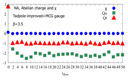
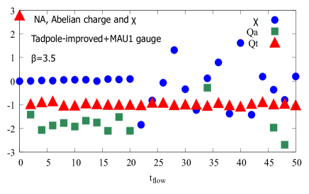
Figure 6: $Q_{t}$, $Q_{a}$ and $\chi$ versus gradient flow time in a configuration at $\beta=3.5$ in MCG (top) and in MAU1 (down).

III.2 Evaluation of the topological charge and its Abelian counterpart

When the additional term is zero, two ways of defining the topological charge $Q_{t}$ are used so farAlexandrou:2020 , i.e., the fermionic definition using (9) and the bosonic definition using (6). The former is always integer when the lattice Dirac operator satisfies the Ginsparg-Wilson relationGW:1982 as in the overlap Dirac operatorNeuberger:1998 . However to get integer values from bosonic definition is not so easy. Various improvements are needed to get a stabilized value as shown for example in Alexandrou:2020 ; Tanizaki:2024 . Here we choose the DBW2 actionDBW2:2000 following Tanizaki:2024 , since it seems best to get a stable $Q_{t}$ rapidly. As the definition of the lattice $Q_{t}$, here we adopt those composed of $1\times 1$ Wilson loops for simplicity. Adopting only 10 configurations at each $\beta$, only one configuration at $\beta=3.5$ gives us a stabilized $Q_{t}$. Hence here we pay attention to the configuration and study the flow-time history up to $\tau=50$ as done in Tanizaki:2024 . Here also we measure the Abelian candidate of the topological charge $Q_{a}$ obtained from (7).

On the lattice, we adopt an Abelian $1\times 1$ plaquette variable as the compact form $f^{L}_{\mu\nu}(s)=Im(\exp(i\theta_{\mu\nu}(s)))$ of Eq.(14). See Fig6. Although non-Abelian $Q_{t}$ becomes stabilized when $\tau>2$, the Abelian $Q_{a}$ are fluctuating between -2 and -3 in MCG gauge. It should become -3 theoretically when the definition would be correct. In MAU1 gauge case, $Q_{a}$ is smaller around -2. Moreover, very unstable behaviors start above $\tau>20$ with respect to both $Q_{a}$ and $\chi$. More elaborate calculations on much larger lattices for larger $\beta$ must be needed along with an additional introduction of smoothing techniques like the block-spin transformation and improved definitions of $Q_{a}$ must be done. It will be a future work.

IV Final comments

1. When the additional term $\chi$ becomes vanishing, we get $Q_{a}=3Q_{t}$ theoretically. This is similar to the Abelian dominance of the string tension. The non-Abelian string tension $\sigma$ is regarded as an average over the string tensions $\sigma_{a}^{i}\ \ (i=1\sim 3)$ of the three colored Abelian fluxes in $SU(2)$. When the global color symmetry is kept, $\sigma_{a}^{1}=\sigma_{a}^{2}=\sigma_{a}^{3}$. The Abelian dominance says $\sigma=\sigma_{a}^{i}$ and so $\sum_{i}\sigma_{a}^{i}=3\sigma$. The non-Abelian topologically charge $Q_{t}$ may be understood similarly.

2. The block-spin transformation used in Abelian monopoles can be expressed also with respect to the Abelian field strength as

   $$\bar{\theta}_{\rho\sigma}^{(n)}(s_{n}) = \sum_{i,j=0}^{n-1}\bar{\theta}_{\rho\sigma}(ns_{n}+i\hat{\rho}+j\hat{\sigma}),$$

   where $s_{n}$ is a site number of the blocked latticeShiba:1994db . The Abelian counterpart of the topological charge $Q_{a}$ is written in terms of the Abelian field strength. Hence using this block-spin transformation on larger lattices for various coupling constants are very interesting in search for the stabilization of $Q_{a}$.

3. The above lattice numerical studies as well as the gradient flow considerations strongly suggest the existence of the continuum limit of Abelian monopoles due to VNABI. However it is known that gauge fields giving Abelian monopoles have a Dirac string with a line singularity and field strengths have a point-like singularityDirac:1931 . There must be some mechanism in QCD therefore admitting existence of Abelian monopoles in the continuum. The problem was discussed already in the worksChernodub:2001A ; Bornyakov:2002 ; Chernodub:2003A . With respect to the Dirac string, it cost no action on the lattice formulated in terms of a compact link field. They showed that it is possible to extend the continuum naive QCD action in such a way to allow for the Dirac strings without any cost in the action. With respect to the point-like singularity, the entropy factor of the monopoles is important in addition to the energy. Compatibility with the asymptotic freedom of QCD needs a fine-tuning between the energy and the entropy. The numerical data on the lattice seem to show the fine-tuning. Our discussions here assume that a similar mechanism is working and topology of QCD can be discussed under the existence of VNABI.

4. VNABI as Abelian monopoles can explain the numerical resultsSuzuki:2008 ; Suzuki:2009 of the perfect monopole dominance without any Abelian projection naturally. However, in order to discuss the Abelian dual Meissner effect in non-Abelian QCD, it is necessary to adopt a $U(1)$ ($U(1)^{2}$) electric subgroup from $SU(2)$ ($SU(3)$). When Abelian monopoles as VNABI condense in the vacuum, monopoles with all color components condense, since there is color invariance. This means that we can adopt any Abelian electric $U(1)$ equally with respect to the Abelian dual Meissner effect. It is the reason that the Abelian dual Meissner effect due to VNABI can explain non-Abelian color confinement of QCD. Although there are $U(1)_{m}^{3}$ symmetries in $SU(2)$, only one $U(1)_{e}$ is the maximal Abelian torus group. When the Abelian monopole $k_{\mu}^{3}$ make condensation for example, electric charged states with respect to $U(1)_{e}^{(3)}$ are confined. However, the state

   $$(\bar{u}_{3}u_{3}-\bar{d}_{3}d_{3})$$ (18)

   which belongs to the $SU(2)$ triplet is not confined, since it is neutral with respect to $U(1)_{e}^{(3)}$. But there are other two $U(1)_{e}$, that is , $U(1)_{e}^{(1)}$ described as $e^{i\alpha_{1}(x)\sigma_{1}}$ and $U(1)_{e}^{(2)}$ described as $e^{i\alpha_{2}(x)\sigma_{2}}$. Then the quark fields having an electric charge $\pm g/2$ with respect to these $U(1)_{e}^{(1)}$ or $U(1)_{e}^{(2)}$ are expressed in terms of $(u_{3},d_{3})$ as $\displaystyle\left(\begin{array}[]{c}u_{1}\\ d_{1}\end{array}\right)=\left(\begin{array}[]{c}\frac{(u_{3}+d_{3})}{\sqrt{2}}\\ \frac{(u_{3}-d_{3})}{\sqrt{2}}\end{array}\right).$ $\displaystyle\left(\begin{array}[]{c}u_{2}\\ d_{2}\end{array}\right)=\left(\begin{array}[]{c}\frac{(iu_{3}+d_{3})}{\sqrt{2}}\\ \frac{(iu_{3}-d_{3})}{\sqrt{2}}\end{array}\right).$

   Since $\bar{u}_{3}u_{3}-\bar{d}_{3}d_{3}=\bar{u}_{1}d_{1}+\bar{d}_{1}u_{1}$, the state (18) is charged with respect to $U(1)_{e}^{1}$ and is confined when the Abelian monopole $k_{\mu}^{1}(x)$ make condensation.

   When monopole condensation occurs in all three-color directions, physical states become $SU(2)$ color singlets alone. Hence non-Abelian $SU(2)$ color confinement is proved by means of the dual Meissner effect caused by Abelian monopoles for all color channels.

5. The above discussions show that Abelian color magnetic monopoles and the Abelian scenario might explain the topological features concerning the vacuum transition and the anomalous chiral $U(1)$ symmetry even without instantons. What happens about the usual chiral $SU(2)\times SU(2)$ symmetry breaking without instantons? There are works suggesting a strong correlation between Abelian magnetic monopoles and the chiral condensateOhta:2021 and Suganuma:2021 .

6. When the gauge field has a line-like singularity in $QED$, there can exist a monopole called Dirac monopoleDirac:1931 . However, such a monopole is not found experimentallyATLAS:2024 . We propose VNABI as Abelian magnetic monopoles assuming the existence of a Dirac-type singularity in non-Abelian gauge fields. To search for the existence of such Abelian monopoles in experiments are very important. The spontaneously broken dual $U(1)^{m}$ predicts existence of color singlet scalar bosons and axial vector dual gauge bosons. It is highly necessary to analyse ADME in dynamical $SU(3)$ QCD to analyse properties including masses of these new boson.

7. Monopoles are expected to play a key role in confinement-deconfinement transition of the universe. It is very interesting to study the mechanism and the role of the monopoles at $T>T_{c}$ is also very interesting in the framework of dynamical full QCD (See a preliminary workBornyakov:2005 ).

8. Usual quantum field theories are based on the axiomatic field theory based on Wightman axioms. There a quantum field is regarded as an operator valued distribution and the derivative of the field operator is defined by the partial derivative with respect to the smooth test function. Hence usually VNABI is not allowed in the framework. If the Dirac monopole or the Abelian monopoles corresponding to VNABI exist, we have to extend the framework of the axiomatic field theory. This is a challenge in the field of mathematical physics.

References

- (1) T. Suzuki, K Ishiguro, Y. Koma and T. Sekido, Phys. Rev. D77, 034502 (2008).
- (2) T. Suzuki et. al., Phys. Rev. D80, 054504 (2009).
- (3) T. Suzuki, arXiv:1402.1294, (2014).
- (4) T. Suzuki, K. Ishiguro and V. Bornyakov, Phys. Rev. D97, 034501 (2018).
- (5) C. Bonati, A. Di Giacomo, L. Lepori and F. Pucci, Phys. Rev. D81, 085022 (2010).
- (6) G. ’t Hooft, Nucl. Phys. B190, 455 (1981).
- (7) P. Dirac, Proc. Roy. Soc. (London) A 133, 60 (1931).
- (8) Y Nambu, Phys. Rev. D10, 4262 (1974).
- (9) S. Mandelstam, Phys. Rept. 23, 245 (1976).
- (10) G. ’t Hooft, in Proceedings of the EPS International, edited by A. Zichichi, p. 1225, 1976.
- (11) K. G. Wilson, Phys. Rev. D10, 2445 (1974).
- (12) T. Suzuki and I. Yotsuyanagi, Phys. Rev. D42, 4257 (1990).
- (13) A. S. Kronfeld, M. L. Laursen, G. Schierholz, and U. J. Wiese, Phys. Lett. B198, 516 (1987).
- (14) A. S. Kronfeld, G. Schierholz, and U. J. Wiese, Nucl. Phys. B293, 461 (1987).
- (15) H. Shiba and T. Suzuki, Phys. Lett. 333B, 461 (1994).
- (16) J. D. Stack, S. D. Neiman and R. J. Wensley, Phys. Rev. D50, 3399 (1994).
- (17) Y. Koma, M. Koma, E.-M. Ilgenfritz and T. Suzuki, Phys. Rev. D68, 114504 (2003).
- (18) T. Sekido et. al., Phys. Rev. D76, 031501 (2007).
- (19) N. Sakumichi and H. Suganuma, Phys. Rev. 90, 111501 (2014).
- (20) K.Ishiguro, A.Hiraguchi and T.Suzuki, Phys Rev D 106 014515 (2022).
- (21) T. Suzuki, Phys Rev D 107, 094503 (2023),
- (22) K. G. Wilson and J. B. Kogut, Phys. Report C12,75 (1974).
- (23) M. Aizenman, Commun. Math. Phys. 86, 1 (1982)
- (24) J. Fröhlich, Nucl. Phys. B200, 281 (1982).
- (25) H. Shiba and T. Suzuki, Phys. Lett. B351, 519 (1995).
- (26) T. Suzuki, Phys. Rev. D97, 034509 (2018).
- (27) T. Suzuki, arXiv:2405.07221(2024).
- (28) A. Belavin, A. Polyakov, A. Schwartz and Y. Tyupkin, Phys. Lett. 59B, 85 (1975).
- (29) M. Müller-Prussker, Lecture note Topology and the QCD vacuum in STRONGnet Summer School 2011 at ZiF Bielefeld, June 2011.
- (30) K. Fujikawa, Phys. Rev. Lett. 42, 1195 (1979).
- (31) L. Alvarez-Gaumé and P. Ginsparg, Nucl. Phys. B243, 449 (1984)
- (32) G. Schierholz, arXiv:2403.13508 (2024).
- (33) A. Hook, arXiv:1812.02669 (2021).
- (34) M. Lüscher, Communic. Math. Phys. 85, 39 (1982).
- (35) M. G. Alford, W. Dimm, G. P. Lepage, G. Hockney, and P. B. Mackenzie, Phys. Lett. B 361, 87 (1995).
- (36) T. A. DeGrand and D. Toussaint, Phys. Rev. D22, 2478 (1980).
- (37) L. Del Debbio, M. Faber, J. Greensite and S. Olejnik, Phys. Rev. D55, 2298 (1997)
- (38) L. Del Debbio, M. Faber, J. Giedt, J. Greensite and S. Olejnik, Phys. Rev. D58, 094501 (1998)
- (39) M. Faber, J. Greensite and S. Olejnik, JHEP 111, 053 (2001).
- (40) V. G. Bornyakov, D. A. Komarov and M.I. Polikarpov, Phys. Lett. B497, 151 (2001).
- (41) M. Lüscher and P. Weisz, JHEP 02, 051 (2011).
- (42) QCD-TARO Collaboration, P. de Forcrand et al., Nucl. Phys. B577, 263 (2000).
- (43) Y. Tanizaki, A. Tomiya and H. Watanabe, arXiv:2411.14812.
- (44) M. Lüscher, JHEP 08, 071 (2010).
- (45) C. Alexandrou et al., Eur. Phys. J. C80, 424 (2020).
- (46) P. H. Ginsparg and K. G. Wilson, Phys. Rev. D25, 2649 (1982).
- (47) H. Neuberger, Phys. Lett. B417, 141 (1998): ibid B427, 353 (1998).
- (48) M.N. Chernodub et al., Nucl. Phys. B600, 163 (2001).
- (49) V. G. Bornyakov et. al., Phys. Lett. B537, 291 (2002).
- (50) M. N. Chernodub and V. I. Zakharov, Nucl. Phys. B669, 233 (2003).
- (51) H. Ohta and H. Suganuma, Phys. Rev. D 103, 054505 (2021).
- (52) H. Suganuma and H. Ohta, Universe 2021, 7(9), 318.
- (53) ATLAS Collaboration, arXiv:2408:11035.
- (54) V. G. Bornyakov et al., Phys. Rev. D 71, 114504 (2005).