JL1-CD: A New Benchmark for Remote Sensing Change Detection and a Robust Multi-Teacher Knowledge Distillation Framework

Abstract

Deep learning has achieved significant success in the field of remote sensing image change detection (CD), yet two major challenges remain: the scarcity of sub-meter, all-inclusive open-source CD datasets, and the difficulty of achieving consistent and satisfactory detection results across images with varying change areas. To address these issues, we introduce the JL1-CD dataset, which contains 5,000 pairs of 512 × 512 pixel images with a resolution of 0.5 to 0.75 meters. Additionally, we propose a multi-teacher knowledge distillation (MTKD) framework for CD. Experimental results on the JL1-CD and SYSU-CD datasets demonstrate that the MTKD framework significantly improves the performance of CD models with various network architectures and parameter sizes, achieving new state-of-the-art results. The code is available at https://github.com/circleLZY/MTKD-CD.

I INTRODUCTION

Remote sensing image change detection (CD) is a technique used to detect and analyze surface changes by leveraging multi-temporal data [1]. Over the past few decades, it has been extensively studied and has become a crucial tool for Earth surface observation. CD plays a significant role in various fields, including land-use change updates, natural disaster assessment, environmental monitoring, and urban planning.

Early traditional CD methods primarily relied on image processing techniques, detecting changes by directly comparing pixel values or spectral features between multi-temporal images. Examples include Image Differencing[2], Change Vector Analysis (CVA)[3], Principal Component Analysis (PCA)[4], Kauth–Thomas (KT) transforms[5], and Multivariate Alteration Detection (MAD)[6]. While these methods are simple and intuitive, they exhibit limited performance when handling complex change patterns, such as those affected by significant noise, lighting variations, or seasonal differences.

With the rise of machine learning (ML), CD methods began to incorporate feature extraction and classifiers. Common techniques include Support Vector Machines (SVM)[7], Random Forest (RF)[8], K-means clustering[9] and so on. These machine learning approaches significantly improved detection accuracy but heavily relied on high-quality labeled data and manually designed features.

In recent years, the rapid advancement of deep learning (DL) has revolutionized remote sensing CD, delivering substantial performance breakthroughs. DL-based CD methods generally involve three steps: (1) extracting change features from image pairs, (2) generating change maps based on the extracted features, and (3) predicting labels based on the feature maps. Convolutional Neural Networks (CNNs), which achieved remarkable success in image processing, were the first neural network architecture applied to remote sensing CD and remain widely optimized and utilized today [10, 11, 12]. With the introduction of Transformers, some studies have explored their application in CD tasks [13, 14]. More recently, Foundational Model (FM) has emerged as a novel paradigm, aiming to achieve multi-task and multi-domain generalization through large-scale pretraining [15]. There have been works utilizing remote sensing data to fine-tune pretrained models such as Vision Transformers (ViT)[16], Segment Anything Model (SAM)[17], and Contrastive Language-Image Pretraining (CLIP)[18], achieving higher performance in CD tasks [19, 20, 21, 22]. Several semi-supervised methods have also been proposed, further improving CD performance under limited labeled data. Zhang et al.[23] propose a novel multilevel consistency-regularization-based semi-supervised CD approach, incorporating Fourier-based frequency transformation and a dynamic pseudolabel selection scheme to mitigate background noise and improve unlabeled data utilization. Xu et al. [24] introduce a semi-supervised label and embedding consistency network (SS-LEC) for ORSI scene classification, which strategically enforces consistency across augmentations and stages of training. Li et al. [25] propose SemiCD-VL, a VLM-guided semi-supervised change detection method that synthesizes pseudo labels via a mixed change event generation strategy, achieving significant performance gains over FixMatch and SOTA unsupervised methods.

However, DL-based CD methods generally face two major challenges: the scarcity of high-quality, high-resolution, all-inclusive CD datasets and limitations in handling highly dynamic change areas. Although numerous CD datasets have been constructed and proposed, they are often tailored to specific scenarios, which restricts the generalization capabilities of the algorithms. For instance, models trained on datasets focused on human-induced changes often fail to perform effectively when confronted with natural change scenarios. On the other hand, the learning capacity of these models is inherently limited. Most existing algorithms rely on a single-phase training approach, typically end-to-end training, supplemented by techniques such as learning rate decay. While such training strategies can achieve satisfactory results within a constrained range of changes, the models’ performance significantly degrades when addressing scenarios with wide variations in change areas, ranging from no change to complete change.

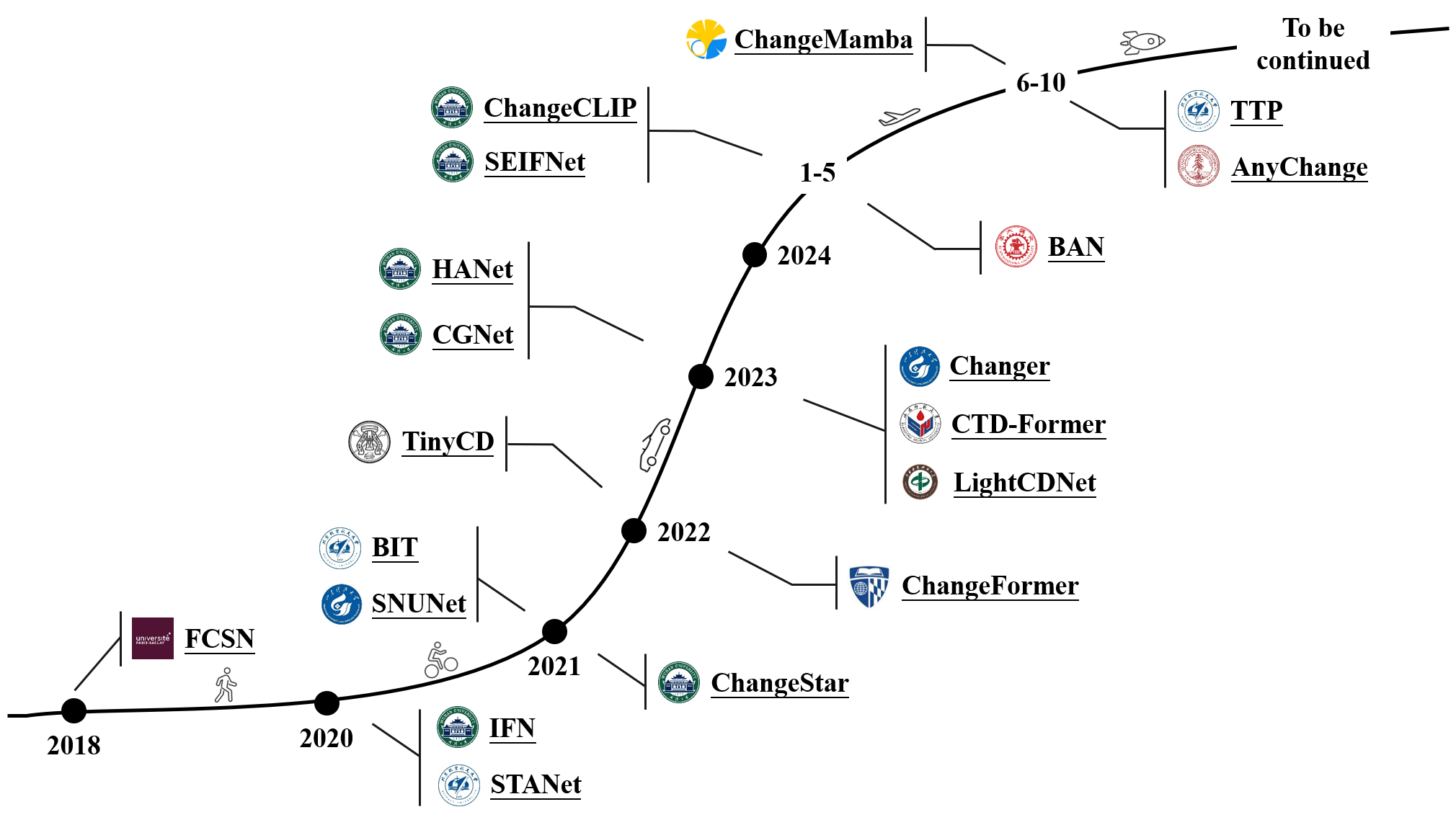
Figure 1: Timeline of the development of mainstream DL-based CD methods.

To address the aforementioned challenges, we construct a new large-scale, high-resolution, all-inclusive open-source CD dataset, named “JL1-CD” (named after the Jilin-1 satellite). This dataset comprises 5,000 pairs of 512 × 512 images captured in China, with a resolution of 0.5–0.75 meters, along with binary change labels at the pixel level. The JL1-CD dataset not only includes common human-induced changes such as buildings and roads but also encompasses various natural changes, such as forests, water bodies, and grasslands. Additionally, we propose a multi-teacher knowledge distillation (MTKD) framework for change detection optimization. First, we introduce the O-P strategy. To address the difficulty of handling highly dynamic change areas in existing algorithms, we propose the concept of the Change Area Ratio (CAR) and partition the dataset based on different CAR levels. CD models are then trained on each partition, reducing the learning burden on individual models, thereby achieving better training outcomes and higher detection accuracy. Next, to lower the computational and time complexity during inference, we extend the O-P strategy by training a student model under the MTKD framework. The student model learns the strengths of teacher models optimized for various CAR scenarios, achieving superior detection accuracy without increasing resource consumption during inference.

Our main contributions are as follows:

1. We introduce JL1-CD, a new sub-meter, all-inclusive open-source CD dataset comprising 5,000 pairs of remote sensing image patches with a resolution of 0.5–0.75 meters.

2. We propose the O-P strategy, which partitions the training of CD models based on CAR levels, significantly improving performance across diverse CAR scenarios.

3. We further develop the MTKD framework, where models trained under the O-P strategy serve as teacher models. The student model trained under the supervision of multiple teachers achieves superior detection accuracy without additional computational or time costs during inference.

4. Extensive benchmarking experiments on existing algorithms demonstrate that O-P and MTKD significantly enhance performance across various architectures and parameter sizes, achieving new state-of-the-art (SOTA) results.

II RELATED WORKS

II-A Traditional and ML-Based CD

Traditional CD methods have been extensively studied in remote sensing, with early approaches relying on simple algebraic operations such as image differencing [2] and image ratioing [26]. These techniques compute pixel-level differences or ratios between two images and apply a threshold to identify change regions. Subsequent advancements introduced improved thresholding strategies, such as the Otsu method [27] and the normalized difference vegetation index (NDVI) algorithm [28], to enhance detection accuracy. Transform-based methods, such as PCA [4] and MAD [6], were later adopted, leveraging statistical properties of images. However, these methods are heavily dependent on image statistics, which limits their scalability and precision in large-scale, high-resolution CD applications. The advent of machine learning has significantly enhanced the ability to extract useful change features. For instance, Bovolo et al. [29] proposed an unsupervised change detection framework that leverages a semi-supervised SVM initialized with pseudo-training data, effectively addressing the complexity of multi-temporal spectral feature analysis. Wessels et al. [30] developed an automated system for land cover update mapping, integrating iteratively reweighted MAD (IRMAD) for change mask generation and RF classifiers for robust land cover classification, achieving notable accuracy in operational settings. Despite these advancements, traditional and early ML-based approaches often rely on manually designed features, which perform well in straightforward scenarios but exhibit limited generalization capability for complex and diverse change types.

II-B DL-Based CD

In recent years, deep learning has experienced rapid advancements, achieving remarkable success in remote sensing image CD. As illustrated in Fig. 1, we present a timeline of the development of mainstream DL-based CD algorithms. Based on the differences in neural network architectures and training paradigms, DL-based CD methods can be classified into three main categories

CNN-Based CD

CNNs serve as the foundation of many early DL-based CD methods and remain widely utilized today. Daudt et al. [10] proposed three fully convolutional neural network architectures, including two Siamese network extensions, which achieved significant improvements in accuracy and efficiency for CD tasks on multiple datasets. Zhang et al. [31] introduced the Image Fusion Network (IFN), which employs a deeply supervised two-stream architecture for high-resolution remote sensing CD, achieving SOTA performance with superior boundary completeness and compactness in change maps. Chen et al. [32] proposed the Siamese-based Spatial-Temporal Attention Network (STANet), incorporating a novel CD self-attention module to model spatial-temporal dependencies at various scales, significantly improving F1-scores on benchmark datasets. Fang et al. [33] designed SNUNet-CD, a densely connected Siamese network that preserves localization information and employs an Ensemble Channel Attention Module (ECAM) for deep supervision, achieving better trade-offs between accuracy and computational cost. Zheng et al. [34] proposed ChangeStar, a model leveraging single-temporal supervised learning with ChangeMixin modules to train CD models using unpaired images. Han et al. [35] introduced HANet, a hierarchical attention network with progressive foreground-balanced sampling and a lightweight self-attention mechanism, effectively addressing class imbalance in CD tasks and achieving superior results on highly imbalanced datasets. The Change Guiding Network (CGNet) introduced by Han et al. [11] utilizes a self-attention mechanism to improve edge detection and internal consistency in change maps, demonstrating robust performance across multiple CD datasets. Some studies have focused on designing lightweight and fast CD models. Codegoni et al. [36] presented TinyCD, a lightweight and efficient CD model using a Siamese U-Net architecture and the Mix and Attention Mask Block (MAMB), outperforming SOTA models while being significantly smaller and faster. Xing et al. [37] proposed LightCDNet, a lightweight CD model with an early fusion backbone and pyramid decoder.

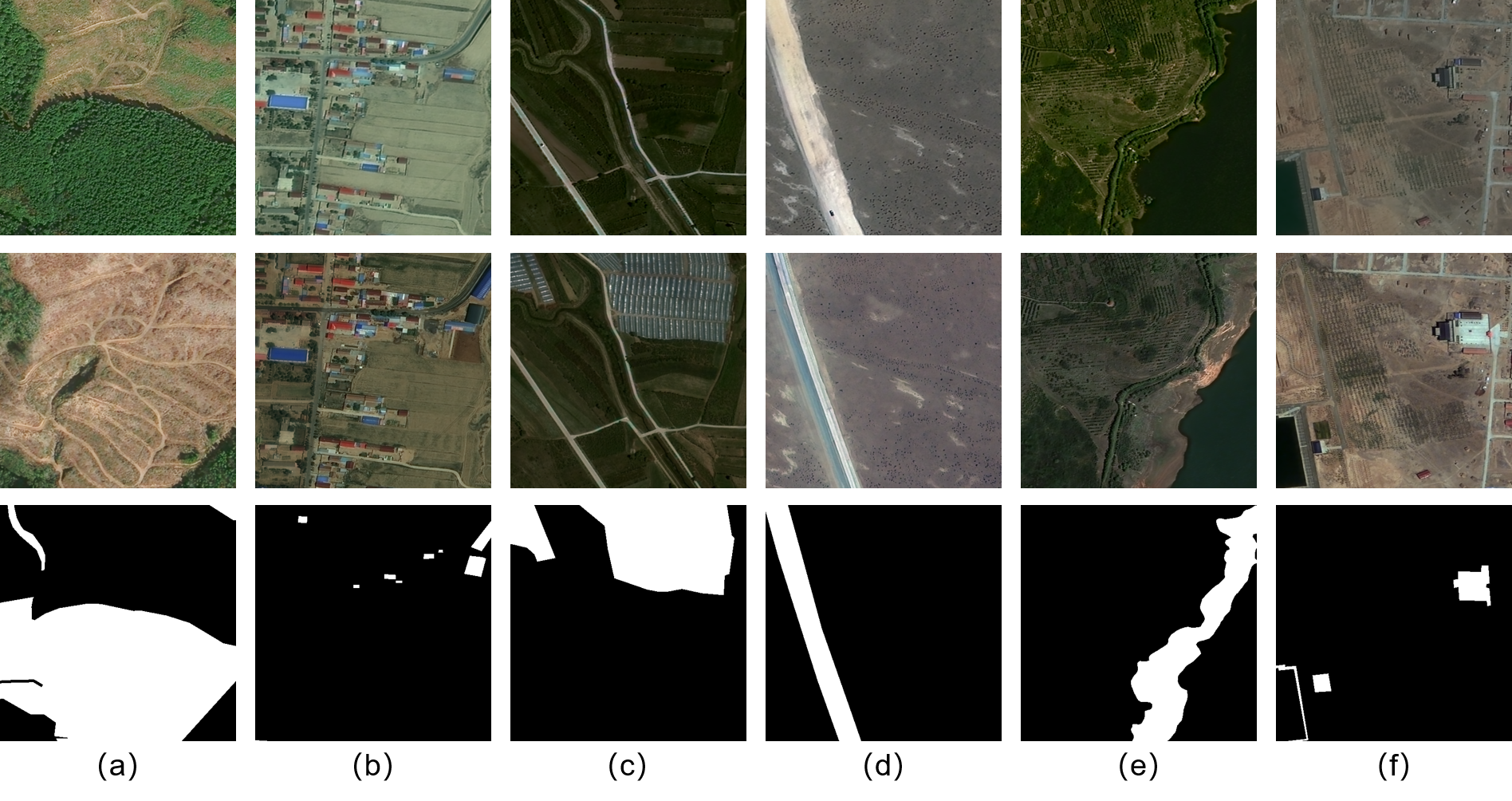
Figure 2: Sample images from the JL1-CD dataset. Each row, from top to bottom, represents: the image at time 1, the image at time 2, and the ground truth label. Each column corresponds to different change types: (a) Decrease in woodland; (b) Building changes; (c) Conversion of cropland to greenhouses; (d) Road changes; (e) Waterbody changes; and (f) Surface hardening (central region).

Transformer-Based CD

Transformer-based methods have emerged as a promising approach for CD. Chen et al. [38] introduced the bitemporal image transformer (BIT), combining a transformer encoder with a ResNet backbone to model spatial-temporal contexts efficiently. Bandara et al. [13] proposed ChangeFormer, a fully transformer-based Siamese network for CD, which unifies a hierarchical transformer encoder with a multi-layer perceptron (MLP) decoder. Fang et al. [14] introduced the Changer series framework, a novel architecture for CD that incorporates alternative interaction layers between bi-temporal features. This framework is applicable to both CNN-based and Transformer-based models, significantly enhancing the performance of the original models.

FM-Based CD

Recently, foundation models have become a new training paradigm, and some works have applied them to CD tasks. Li et al. [19] proposed the Bi-Temporal Adapter Network (BAN), a universal FM-based framework for CD, which enhances existing models with minimal additional parameters and achieves significant performance improvements. Chen et al. [21] introduced Time Travelling Pixels (TTP), a method that integrates latent knowledge from the SAM model into CD, overcoming domain shifts and spatio-temporal complexities, demonstrating SOTA results on the LEVIR-CD[32] dataset. Zheng et al. [22] developed AnyChange, a zero-shot CD model built on the SAM that utilizes bitemporal latent matching for training-free adaptation, setting a new SOTA on the SECOND[39] benchmark and achieving significant improvements in both unsupervised and supervised CD tasks.

II-C Knowledge Distillation in CD

Knowledge distillation (KD), introduced by Hinton et al. [40], aims to transfer the representational knowledge of a teacher network to a smaller student network. In recent years, as the complexity of DL models in remote sensing tasks has increased, researchers have explored how to transfer knowledge from large, complex teacher models to smaller, more efficient student models through KD, thereby improving performance[41, 42].

Yan et al. [43] proposed a novel self-supervised learning approach for unsupervised CD by fusing domain knowledge of remote sensing indices during both training and inference. By calculating cosine similarity, they selected high-similarity feature vectors from both the teacher and student networks to implement a hard negative sampling strategy, effectively improving CD performance. Wang et al. [44] addressed remote sensing semantic CD (SCD), which focuses on detecting changes in land cover and land use over time. The authors introduced a dual-dimension feature interaction network (DFINet) that enhances intraclass and interclass feature differentiation by incorporating a temporal difference feature enhancement (TDFE) module, which captures temporal features comprehensively. Wang et al. [45] proposed a KD-based method for CD (CDKD), designed to overcome the challenges of deploying large deep learning models with high computational and storage requirements on resource-constrained spaceborne edge devices. Although these methods have successfully utilized KD to enhance the performance of various student models, they are tailored to specific models and do not provide a generalized distillation framework applicable to various CD models. Furthermore, there is a lack of open-source KD-based code for remote sensing image CD tasks.

In contrast, the proposed MTKD framework significantly improves the performance of CD models with various architectures and parameter sizes, and we commit to open-sourcing all the code and models.

TABLE I: Information of Open-Source CD Datasets and the Proposed JL1-CD Dataset

Dataset	Class	Image Pairs	Image Size	Resolution
SZTAKI[46]	1	13	$952\times 640$ $1,048\times 724$	1.5
DSIFN[31]	1	394	512 × 512	2
SECOND[39]	6	4,662	512 × 512	0.5-3
WHU-CD[47]	1	1	32,20 × 15,354	0.2
LEVIR-CD[32]	1	637	1,024 × 1,024	0.3
S2Looking[48]	1	5,000	1,024 × 1,024	0.5-0.8
CDD[49]	1	16,000	256 × 256	0.03-1
SYSU-CD[50]	1	20,000	256 × 256	0.5
JL1-CD	1	5,000	512 × 512	0.5-0.75

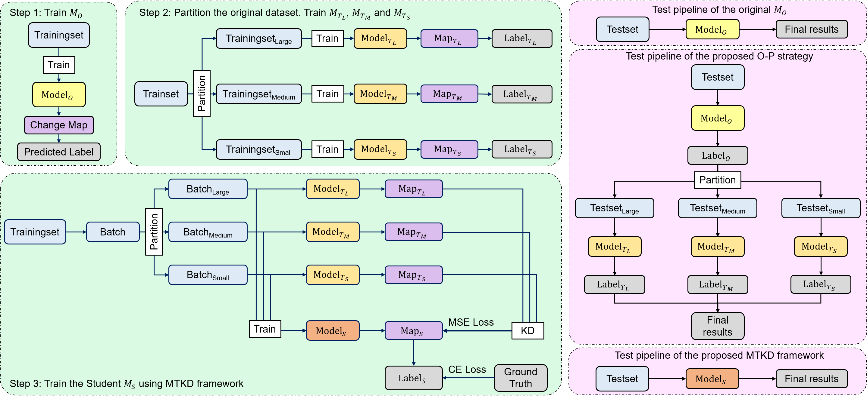
Figure 3: Overview of the training (green boxes) and testing (pink boxes) pipelines of the proposed Origin-Partition (O-P) strategy and Multi-Teacher Knowledge Distillation (MTKD) framework.

III JL1-CD Dataset

High-resolution, all-inclusive CD datasets are crucial for remote sensing applications. High-resolution images provide richer spatial information, which is more conducive to visual interpretation compared to medium- and low-resolution images. Datasets with comprehensive change features enable the development of algorithms with greater generalization and transferability. Despite the numerous open-source change detection datasets proposed over the past decades, many still lack sub-meter-level resolution, and the variety of change types remains limited. These limitations hinder progress in CD research, particularly in the development of DL-based algorithms.

We collect the number of types of changes, number of image pairs, image size, and resolution information of mainstream CD datasets in Table I. The SZTAKI AirChange Benchmark [46] contains 12 pairs of 952 × 640 and one pair of 1,048 × 724 optical aerial images. It is one of the earliest and most commonly used CD datasets in early research. The DSIFN dataset [31] consists of 6 large bi-temporal image pairs from 6 cities in China, which are cropped into 394 sub-image pairs, each sized 512 × 512. The SECOND dataset [39] includes 4,662 pairs of aerial images collected from multiple platforms and sensors, covering cities such as Hangzhou, Chengdu, and Shanghai. Unlike other datasets that classify changes into only two categories (change and no change), SECOND provides detailed annotations for change types, including non-vegetated surfaces, trees, low vegetation, water, buildings, and playgrounds. However, the resolution of all or part of the images in these datasets does not reach the sub-meter level. WHU-CD [47], LEVIR-CD [32], and S2Looking [48] are very popular datasets that are specifically designed for monitoring building changes. These datasets predominantly include human-induced changes and lack natural change types. The CDD dataset is derived from 7 pairs of 4,725 × 2,700 real-world seasonal change remote sensing images. The SYSU-CD contains 20,000 pairs of 0.5-meter aerial images captured in Hong Kong between 2007 and 2014. These datasets feature high resolution and diverse change types.

To provide a better benchmark for evaluating CD algorithms, we propose the JL1-CD dataset, a high-resolution, all-inclusive change detection dataset. JL1-CD includes 5,000 pairs of satellite images captured in China from early 2022 to the end of 2023, including Shandong, Ningxia, Anhui, Hebei, Hunan, and other regions. The images have sub-meter resolutions ranging from 0.5 to 0.75 meters and are sized 512 × 512 pixels. As shown in Fig. 2, the dataset covers various common human-induced and natural surface features, such as piled earth, buildings, roads, hardened surfaces, woodlands, grasslands, croplands, and water bodies. The original 5,000 image pairs are divided into 4,000 pairs for training and 1,000 pairs for testing, following an 80:20 split. The JL1-CD dataset will be made openly available for all research needs.

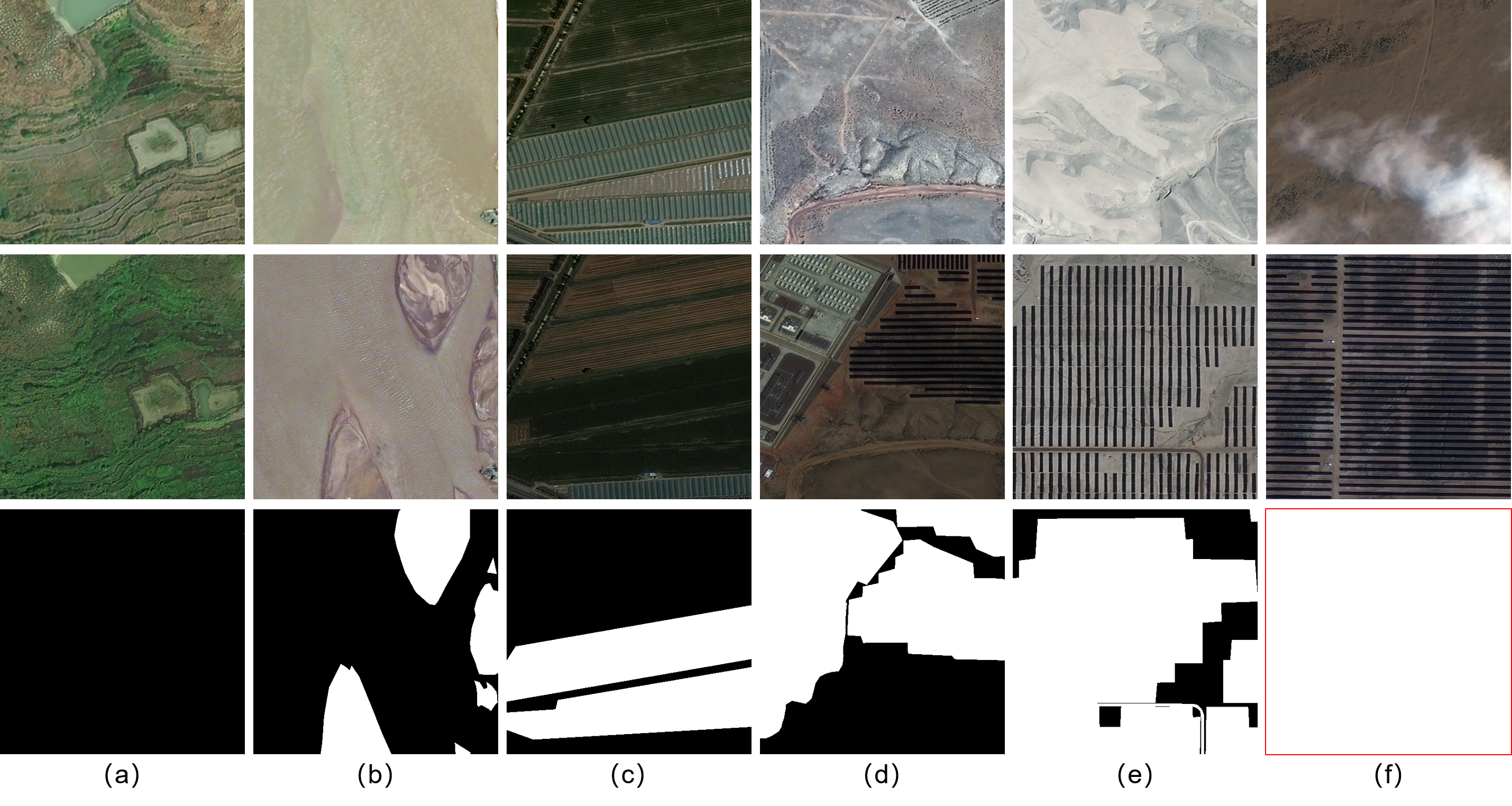
Figure 4: Sample images with different change area ratios (CAR). Each column represents a specific CAR: (a) 0.00%; (b) 19.98%; (c) 39.93%; (d) 59.96%; (e) 80.25%; and (f) 100.00%.

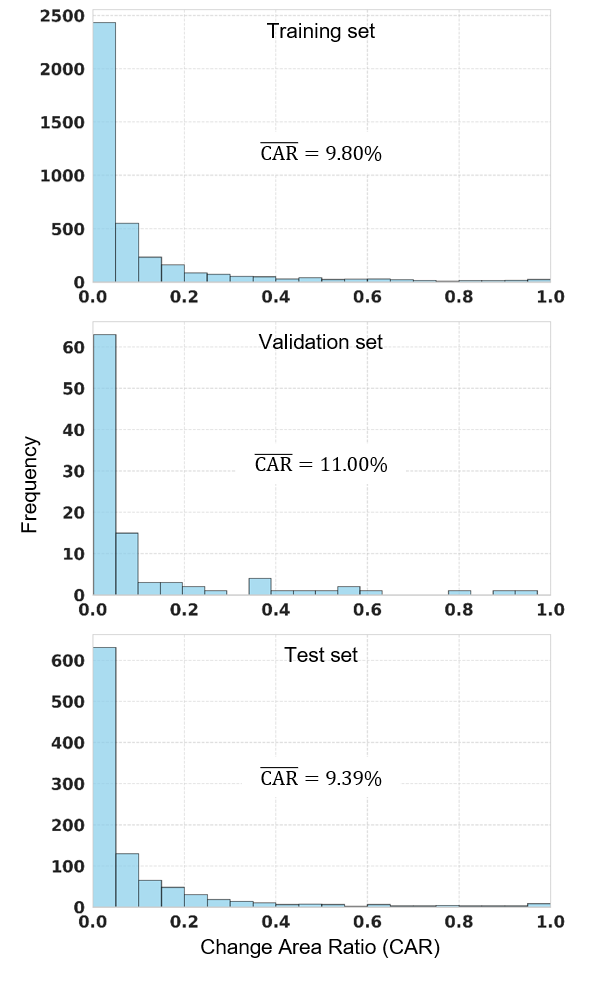
Figure 5: CAR distribution of the training, validation and test sets in JL1-CD.

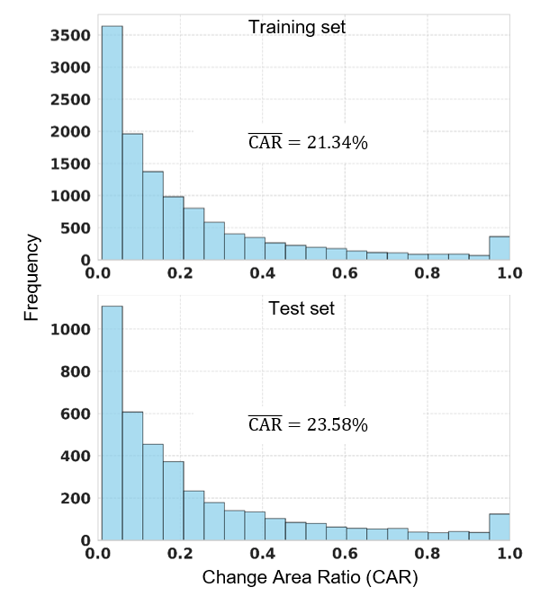
Figure 6: CAR distribution of the training and test sets in SYSU-CD.

IV Methodology

In this section, we provide a comprehensive overview of the proposed methods. In Section IV-A, we first introduce the Origin-Partition (O-P) strategy designed for the challenging all-inclusive CD dataset. Building upon the O-P strategy, we further present our Multi-Teacher Knowledge Distillation (MTKD) framework in Section IV-B. Finally, in Section IV-C, we describe the overall loss function used for training the teacher and student models.

IV-A O-P Strategy

The traditional training and testing approach for CD models is illustrated in the upper-left corner of Fig. 3 (green box) and the upper-right corner (pink box). For a given change detection model $\mathcal{M}$, the input consists of a pair of images $(X_{1},X_{2})$, and the output is a change map (CM). If the number of channels $c=1$, the predicted label $\hat{Y}$ can be directly obtained using a thresholding method as follows:

$$\hat{Y}(i)=\begin{cases}1,&\text{if }CM(i)>th\\ 0,&\text{if }CM(i)\leq th\end{cases}$$ (1)

where $(i)$ denotes the pixel location in the image, ”1” represents a change, and ”0” represents no change (for visualization purpose, ”1” will be mapped to a grayscale value of 255). The threshold $th$ is a predefined value. If $c=2$, the predicted label $\hat{Y}$ is typically determined using an element-wise comparison of the two channels, such as:

$$\hat{Y}(i)=\begin{cases}1,&\text{if }CM_{0}(i)\geq CM_{1}(i)\\ 0,&\text{if }CM_{0}(i)<CM_{1}(i)\end{cases}$$ (2)

where $CM_{0}$ and $CM_{1}$ represent the first and second layers of the change map, respectively. If $c>2$, it indicates that the CD model $\mathcal{M}$ not only predicts the locations of changes but also detects the types of changes, which is beyond the scope of this paper.

However, as shown in Fig. 4, for a dataset like JL1-CD, where the Change Area Ratio (CAR) can range from 0% to 100%, training a single model using traditional methods may not be optimal. The model would struggle to learn the full range of change patterns in an all-inclusive manner. To address this issue, we propose the Origin-Partition (O-P) strategy to enhance the model’s detection performance. As illustrated in the green boxes of Fig. 3 (Step 1 and Step 2), for a given CD algorithm, we train the corresponding models in the following sequence:

1) The original model $\mathcal{M}_{O}$ is trained on the complete training set using the algorithm’s default configuration.

2) As shown in Fig. 5, the CAR range for the training, validation, and test sets is very large. However, the majority of images have a CAR of less than 5%. Therefore, we set appropriate thresholds $th_{1}$ and $th_{2}$ and divide the original training set into three categories: small, medium, and large.

3) The models are then trained from scratch using the partitioned training sets, yielding models $\mathcal{M}_{T_{S}}$, $\mathcal{M}_{T_{M}}$, and $\mathcal{M}_{T_{L}}$. The training process can be formalized as:

$$\hat{Y}=\begin{cases}f_{\mathcal{M}_{T_{S}}}(X_{1},X_{2}),&\text{if }CAR_{GT}\leq th_{1}\\ f_{\mathcal{M}_{T_{M}}}(X_{1},X_{2}),&\text{if }th_{1}<CAR_{GT}\leq th_{2}\\ f_{\mathcal{M}_{T_{L}}}(X_{1},X_{2}),&\text{if }CAR_{GT}>th_{2}\end{cases}$$ (3)

where $CAR_{GT}$ denotes the CAR calculated based on the ground truth label for the image pair $(X_{1},X_{2})$.

As shown in the middle pink box in Fig. 3, during testing, since we do not know the CAR of the test images, we first use $\mathcal{M}_{O}$ to estimate the CAR roughly. Based on this estimated CAR, we then classify the image into one of the three categories: small, medium, or large, and send it to the corresponding model $\mathcal{M}_{T_{S}}$, $\mathcal{M}_{T_{M}}$, or $\mathcal{M}_{T_{L}}$ to obtain the final detection result:

$$\hat{Y}=\begin{cases}f_{\mathcal{M}_{T_{S}}}(X_{1},X_{2}),&\text{if }CAR_{\mathcal{M}_{O}}\leq th_{1}\\ f_{\mathcal{M}_{T_{M}}}(X_{1},X_{2}),&\text{if }th_{1}<CAR_{\mathcal{M}_{O}}\leq th_{2}\\ f_{\mathcal{M}_{T_{L}}}(X_{1},X_{2}),&\text{if }CAR_{\mathcal{M}_{O}}>th_{2}\end{cases}$$ (4)

where $CAR_{\mathcal{M}_{O}}$ denotes the CAR calculated based on the predicted label from the original model $\mathcal{M}_{O}$.

IV-B MTKD Framework

By partitioning the training set, we effectively reduce the learning burden for each model. As a result, the Origin-Partition (O-P) strategy significantly enhances the performance of the CD algorithm. However, a clear issue arises: during inference, we are required to load 4 different models, and even disregarding data throughput, the time spent is at least twice that of the original algorithm (often much more). This substantially increases both memory and time complexity. We are thus prompted to consider: is there a way to combine the capabilities of these four models into a single model?

To address this, we propose the Multi-Teacher Knowledge Distillation (MTKD) framework. In the O-P strategy, we have already trained the models $\mathcal{M}_{O}$, $\mathcal{M}_{T_{S}}$, $\mathcal{M}_{T_{M}}$, and $\mathcal{M}_{T_{L}}$. Building on this, we further train a student model $\mathcal{M}_{S}$. First, we initialize the student model $\mathcal{M}_{S}$ using the parameters from $\mathcal{M}_{O}$, and then use $\mathcal{M}_{T_{S}}$, $\mathcal{M}_{T_{M}}$, and $\mathcal{M}_{T_{L}}$ as teacher models to perform KD. For each input image pair, we select the appropriate teacher model based on the image’s CAR to guide the student model. The process is shown in the green box at the bottom of Fig. 3. In this framework, when the student model $\mathcal{M}_{S}$ is supervised by the ground truth labels, it also receives the CM information corresponding to different CAR ranges, provided by the teacher models.

During the testing phase, only the student model $\mathcal{M}_{S}$ is used for inference, thereby significantly improving the model’s CD performance across different CAR ranges without introducing any additional computational cost.

IV-C Loss Function

When training the original model $\mathcal{M}_{O}$ and the teacher models $\mathcal{M}_{T_{S}}$, $\mathcal{M}_{T_{M}}$, and $\mathcal{M}_{T_{L}}$, we employ the standard binary cross-entropy loss:

$$L_{\text{CE}}=\frac{1}{N}\sum_{i=1}^{N}(-Y(i)\log(\hat{Y}(i))-(1-Y(i))\log(1-\hat{Y}(i)))$$ (5)

where $Y(i)$ denotes the ground truth label of pixel $i$.

When training the student model $\mathcal{M}_{S}$, we select the appropriate teacher model based on the CAR range. Then the mean squared error (MSE) is computed at the CM layer as the distillation loss:

$$L_{\text{KD}}=\frac{1}{N}\sum_{i=1}^{N}\left(CM(i)-CM_{\mathcal{T}}(i)\right)^{2},\quad\mathcal{T}\in\{T_{S},T_{M},T_{L}\}.$$ (6)

Thus, the complete loss function for training $\mathcal{M}_{S}$ is given by:

$$L=L_{\text{CE}}+\lambda L_{\text{KD}}$$ (7)

where the parameter $\lambda$ is used to balance the contributions of the cross-entropy loss and the distillation loss.

TABLE II: Benchmark Methods and the Corresponding Implementation Details

Method	Backbone	Param (M)	Flops (G)	Initial LR	$\lambda$	Scheduler	Batch Size	GPU
FC-EF[10]	CNN	1.353	12.976	1e-3	-	LinearLR	8	3090
FC-Siam-Conc[10]	CNN	1.548	19.956	1e-3	-	LinearLR	8	3090
FC-Siam-Diff[10]	CNN	1.352	17.540	1e-3	-	LinearLR	8	3090
STANet-Base[32]	ResNet-18	12.764	70.311	1e-3	5e-3	LinearLR	8	3090
IFN[31]	VGG-16	35.995	323.584	1e-3	1e-4	LinearLR	8	3090
SNUNet-c16[33]	CNN	3.012	46.921	1e-3	1e-4	LinearLR	8	3090
BIT[38]	ResNet-18	2.990	34.996	1e-3	1e-4	LinearLR	8	3090
	FarSeg (ResNet-18)[51]	16.965	76.845	1e-3	1e-3	LinearLR	16	3090
ChangeStar[34]	UPerNet (ResNet-18)[52]	13.952	55.634	1e-3	1e-4	LinearLR	8	3090
	MiT-b0	3.847	11.380	6e-5	1e-3	LinearLR	8	3090
ChangeFormer[13]	MiT-b1	13.941	26.422	6e-5	5e-4	LinearLR	8	3090
TinyCD[36]	CNN	0.285	5.791	3.57e-3	1e-5	LinearLR	8	3090
HANet[35]	CNN	3.028	97.548	1e-3	1e-3	LinearLR	8	A800
	MiT-b0	3.457	8.523	1e-4	1e-4	LinearLR	8	3090
	MiT-b1	13.355	23.306	1e-4	1e-3	LinearLR	8	3090
	ResNet-18	11.391	23.820	5e-3	1e-3	LinearLR	8	3090
Changer[14]	ResNeSt-50	26.693	67.241	5e-3	1e-5	LinearLR	8	3090
LightCDNet-s[37]	CNN	0.342	6.995	3e-3	5e-3	LinearLR	8	3090
CGNet[11]	VGG-16	38.989	425.984	5e-4	1e-3	LinearLR	8	A800
	ViT-B	91.346	74.409	1e-4	-	LinearLR	8	3090
	ViT-B (IN21K)	115.712	83.142	1e-4	-	LinearLR	8	3090
BAN[19]	ViT-L	261.120	346.112	1e-4	1e-3	LinearLR	8	A800
TTP[21]	SAM[17]	361.472	929.792	4e-4	5e-3	CosineAnnealingLR	8	A800

TABLE III: Experimental Results on JL1-CD Test Set

Method	Strategy	mIoU	mAcc	mPrecision	mFscore		Method	Strategy	mIoU	mAcc	mPrecision	mFscore
STANet (Base)	-	66.76	81.71	74.73	74.73		IFN	-	71.25	78.91	84.53	77.33
	O-P	64.56	78.47	78.47	71.25			O-P	71.06	78.37	84.28	77.21
	MTKD	67.92	82.07	76.24	75.10			MTKD	72.72	80.28	84.66	78.80
SNUNet (c16)	-	68.97	74.87	85.06	75.25		BIT	-	67.22	74.47	83.71	73.37
	O-P	71.39	78.60	83.36	77.98			O-P	69.41	76.29	84.02	75.77
	MTKD	71.12	78.27	84.96	77.56			MTKD	68.86	75.49	84.71	74.88
ChangeStar (FarSeg)	-	69.47	75.58	84.46	75.57		ChangeStar (UPerNet)	-	64.85	69.18	88.26	70.19
	O-P	68.87	74.74	84.90	74.86			O-P	64.68	69.05	87.23	70.08
	MTKD	69.14	76.49	82.09	75.41			MTKD	65.10	70.26	87.69	70.58
ChangeFormer (MiT-b0)	-	73.51	80.46	86.33	79.70		ChangeFormer (MiT-b1)	-	73.05	79.70	86.95	79.22
	O-P	72.58	79.16	86.33	78.79			O-P	73.45	79.19	87.45	79.41
	MTKD	73.25	79.20	87.15	79.30			MTKD	73.92	80.43	86.89	80.18
TinyCD	-	71.04	78.77	83.05	77.74		HANet	-	63.64	69.77	83.43	69.39
	O-P	72.22	79.93	83.49	78.76			O-P	69.05	76.53	83.05	75.66
	MTKD	72.55	80.98	83.17	79.26			MTKD	67.67	74.39	84.38	73.92
Changer (MiT-b0)	-	74.85	81.84	86.09	80.98		Changer (MiT-b1)	-	75.94	81.99	87.74	81.93
	O-P	75.29	81.40	87.06	81.32			O-P	75.42	81.67	87.13	81.43
	MTKD	75.35	81.76	87.18	81.28			MTKD	76.15	82.85	86.98	82.13
Changer (r18)	-	68.37	75.15	83.43	74.54		Changer (s50)	-	62.31	69.23	80.91	67.83
	O-P	70.76	77.42	83.86	77.01			O-P	71.80	79.76	83.15	78.23
	MTKD	69.45	77.26	81.50	75.86			MTKD	62.96	69.65	81.76	68.52
LightCDNet (s)	-	66.70	73.21	83.45	72.46		CGNet	-	73.37	80.31	85.33	79.65
	O-P	70.19	77.43	83.99	76.16			O-P	72.95	79.71	85.50	79.12
	MTKD	65.99	72.44	83.86	71.48			MTKD	73.82	80.32	86.33	79.91
BAN (ViT-L)	-	73.54	79.54	87.89	79.47		TTP	-	75.05	80.24	89.82	80.76
	O-P	73.61	79.17	88.10	79.45			O-P	76.69	83.48	87.27	82.52
	MTKD	73.95	80.26	87.12	79.92			MTKD	76.85	82.99	88.05	82.56
BAN (ViT-B)	-	73.30	80.36	85.91	79.47		BAN (ViT-B-IN21K)	-	74.69	81.09	87.14	80.75
	O-P	72.47	78.78	86.31	78.58			O-P	73.50	79.98	86.25	79.50
FC-EF	-	57.08	61.90	86.40	61.28		FC-Siam-Conc	-	63.79	69.54	84.77	69.19
	O-P	49.59	53.30	95.54	51.47			O-P	60.25	63.84	91.19	64.72
FC-Siam-Diff	-	61.30	66.03	86.45	66.34
	O-P	56.49	60.05	91.64	60.57

V EXPERIMENT

V-A Dataset Description

We first conduct experiments on our JL1-CD dataset. Additionally, to validate the robustness of the proposed O-P strategy and MTKD framework, we further perform experiments on the SYSU-CD dataset [50]. The detailed information for these two datasets is as follows:

1) JL1-CD Dataset: As described in Section III, the JL1-CD dataset consists of 5,000 pairs of high-resolution images, with a resolution of 0.5-0.75 meters and image size of 512 × 512. In the competition, the first 4,000 image pairs are used for training, and the remaining 1,000 image pairs are used for testing (with the ground truth labels being unavailable during the competition). To ensure sufficient data for training, we use the first 100 image pairs as the validation set, the next 3,900 image pairs as the training set, and the remaining 1,000 image pairs for testing. As shown in Fig. 5, our data split is reasonable, as the CAR distributions of the three sets are very similar.

2) SYSU-CD Dataset: As illustrated in Fig. 6, the SYSU-CD dataset is also a challenging dataset with a very large CAR range, so we choose this dataset as the second benchmark to validate the robustness of our proposed methods. The SYSU-CD dataset contains 12,000 pairs for training, 4,000 pairs for validation, and 4,000 pairs for testing, with each image having a resolution of 0.5 meters and a size of 256 × 256.

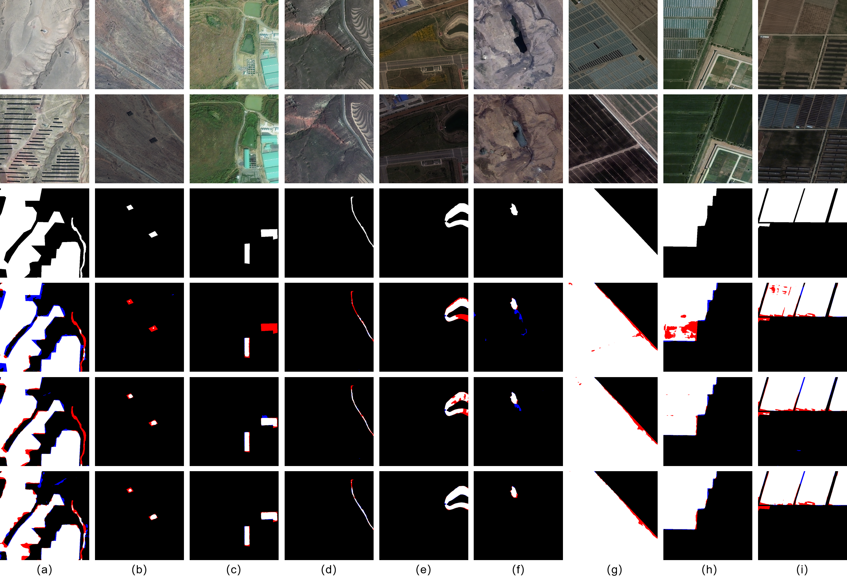
Figure 7: Visual comparison on the JL1-CD dataset. Each row, from top to bottom, represents the following: image at time 1, image at time 2, ground truth, output from the original model, output from the O-P strategy, and output from the MTKD framework. Red denotes missed detections (FN), while blue indicates false alarms (FP). The selected algorithms are: (a) BAN-ViT-L, (b) BIT, (c) TTP, (d) SNUNet, (e) IFN, (f) Changer-MiT-b1, (g) ChangeFormer-MiT-b1, (h) TinyCD, and (i) CGNet.

V-B Benchmark Methods

To comprehensively verify the validity of our JL1-CD dataset and the superiority of the proposed O-P strategy and MTKD framework, we conduct extensive experiments on existing benchmark algorithms. The selected models, along with their corresponding backbones, parameter sizes, and computational complexities, are summarized in Table II. Based on the backbone architecture, the models are categorized into three groups: Alice Blue for CNN-based models, Light Cyan for Transformer-based models, and Lavender Blue for FM-based models, encompassing almost all mainstream architectures. FLOPs is calculated with an input image of size 512 × 512. As shown in the table, the selected models span a wide range of sizes, from lightweight models such as TinyCD and LightCDNet with less than 1MB to the latest SOTA model TTP, which exceeds 360MB. This wide range allows us to verify the universality of the O-P and MTKD methods across models with different backbones and scales.

V-C Evaluation Metrics

The common evaluation metrics for CD models include Intersection over Union (IoU), accuracy, precision, recall, and F1-score. IoU measures the overlap between the detected change region and the ground truth. Accuracy reflects the overall correctness of the model. Precision indicates the false positive rate of the model, recall reflects the false negative rate, and F1-score balances both precision and recall. A higher F1-score indicates better detection performance.

However, given the large CAR range in the JL1-CD dataset, both change and non-change regions are equally important. Therefore, we choose the averaged versions of the aforementioned metrics, which are calculated as follows:

mIoU $$=\frac{1}{2}\left(\text{IoU}_{0}+\text{IoU}_{1}\right)$$ (8)

$$=\frac{1}{2}\left(\frac{\text{TN}}{\text{TN}+\text{FP}+\text{FN}}+\frac{\text{TP}}{\text{TP}+\text{FP}+\text{FN}}\right)$$

mPrecision $$=\frac{1}{2}\left(\text{Precision}_{0}+\text{Precision}_{1}\right)$$

$$=\frac{1}{2}\left(\frac{\text{TN}}{\text{TN}+\text{FN}}+\frac{\text{TP}}{\text{TP}+\text{FP}}\right)$$

mAcc $$=\frac{1}{2}\left(\text{Recall}_{0}+\text{Recall}_{1}\right)$$

$$=\frac{1}{2}\left(\frac{\text{TN}}{\text{TN}+\text{FP}}+\frac{\text{TP}}{\text{TP}+\text{FN}}\right)$$

mFscore $$=\frac{1}{2}\left(\text{Fscore}_{0}+\text{Fscore}_{1}\right)$$

$$=\frac{1}{2}\sum_{i=0}^{1}\frac{2\times\text{Precision}_{i}\times\text{Recall}_{i}}{\text{Precision}_{i}+\text{Recall}_{i}}$$

where TP, FP, TN, and FN represent true positives, false positives, true negatives, and false negatives, respectively. The averaged accuracy and recall are equivalent, so we only use mAcc for consistency in subsequent experiments.

It is important to note that in the toolboxes like MMSegmentation[53] and MMRotate [54], these metrics are computed based on the total number of pixels across all predicted label images. In this paper, however, to align with the competition requirements, we first calculate these metrics for each individual image and then compute the average of the results across all images to obtain the final outcome.

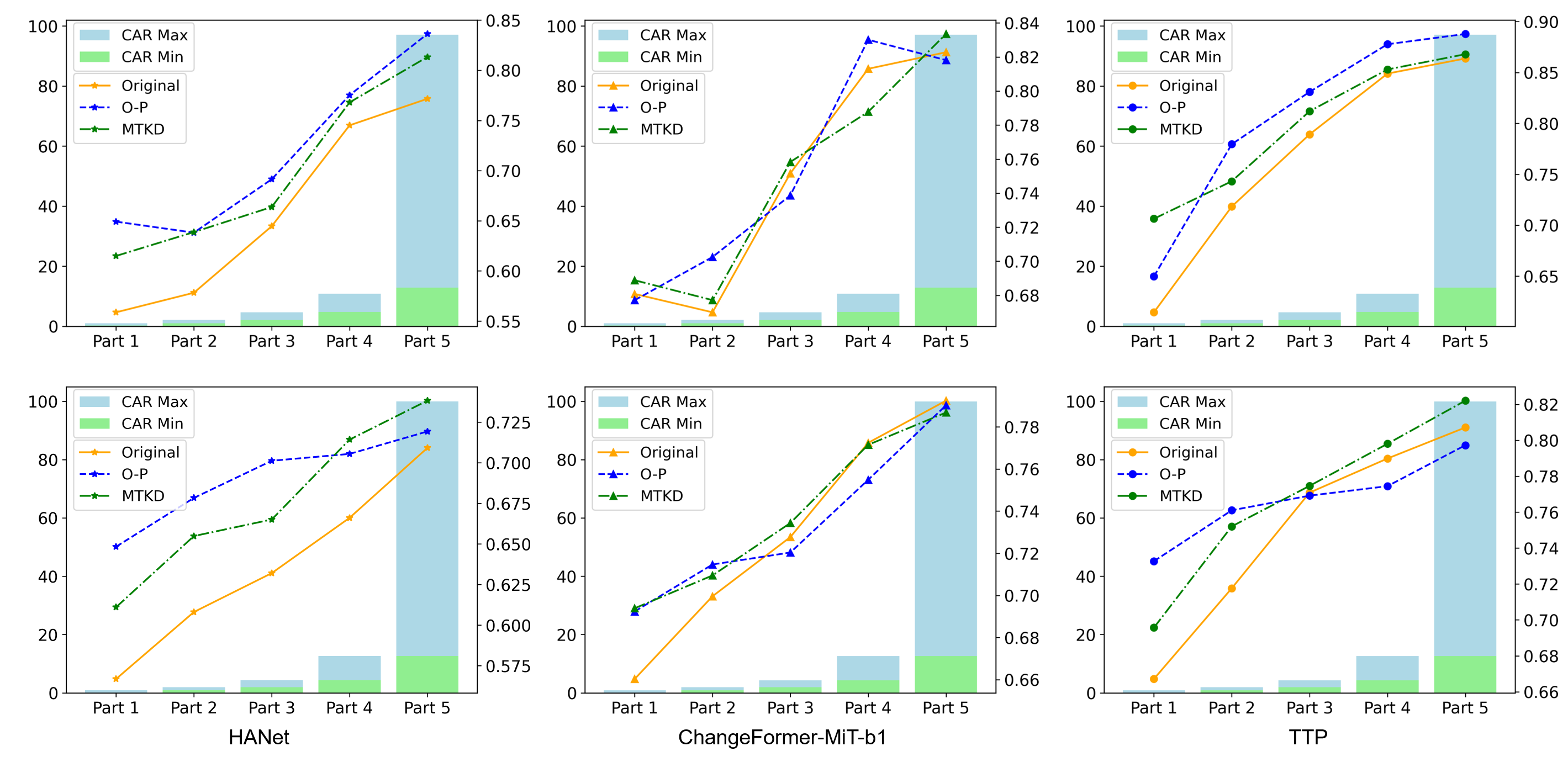
Figure 8: mIoU of HANet, ChangeFormer-MiT-b1, and TTP across different CAR ranges. The first and second rows show results on the validation and test sets, respectively. In each plot, the left y-axis represents CAR size, and the right y-axis represents mIoU.

V-D Implementation Details

All algorithms are trained and tested using the PyTorch-based OpenCD Toolbox [55]. To ensure a fair comparison and clearly assess the contributions of the Origin-Partition (O-P) strategy and the Multi-Teacher Knowledge Distillation (MTKD) framework to the performance improvement of the CD models, we adopt consistent settings for all models ($\mathcal{M}_{O}$, $\mathcal{M}_{T_{L}}$, $\mathcal{M}_{T_{M}}$, $\mathcal{M}_{T_{S}}$, and $\mathcal{M}_{S}$) across the various algorithms, as described below:

1. The patch size of the input images is 512 × 512, which matches the original image dimensions.

2. Data augmentation methods, including RandomRotate, RandomFlip, and PhotoMetricDistortion, are applied.

3. The AdamW optimizer is used with $\beta_{1}=0.9$ and $\beta_{2}=0.99$, and the default batch size is set to 8 image pairs (with a batch size of 16 for ChangeStar-FarSeg).

4. Models $\mathcal{M}_{O}$, $\mathcal{M}_{T_{L}}$, $\mathcal{M}_{T_{M}}$, and $\mathcal{M}_{T_{S}}$ are trained for 200k iterations on the original and the corresponding partitioned datasets (300 epochs for TTP), while the student model $\mathcal{M}_{S}$ is trained for an additional 100k iterations (100 epochs for TTP) on the original dataset.

5. Training begins with a warm-up phase of 1k iterations (5 epochs for TTP), during which the learning rate (LR) is linearly increased from 1e-6 to the initial LR value, as specified in Table II. Afterward, the LR is linearly decayed to 0 as training progresses (TTP employs a CosineAnnealing decay schedule).

6. The HANet, CGNet, BAN (ViT-L), and TTP models are trained on the NVIDIA A800 server, while other models are trained on the NVIDIA RTX 3090 server. All models are tested on the A800 server.

When partitioning the dataset, we set the thresholds $th_{1}=0.05$ and $th_{2}=0.2$, which ensures a balanced distribution of samples across the partitions. The model is saved every 1k iterations (5 epochs for TTP), and the checkpoint with the highest mIoU value on the validation set is selected for testing.

For the training of $\mathcal{M}_{T_{S}}$, due to the varying distributions of the change maps and the different magnitudes of $L_{CE}$ across modelss, a grid search is performed over the set $\{1e-5,5e-5,1e-4,5e-4,1e-3,5e-3,1e-2\}$ to determine the optimal distillation loss weight $\lambda$ for each model. More configuration details are summarized in Table II.

TABLE IV: Comparison of Detection Results on Change and No-Change Classes

Method	Class	IoU	Acc	Precision	Fscore
	unchanged	+0.24	+0.29	+0.04	+0.12
IFN	changed	+2.71	+2.44	+0.22	+2.82
	unchanged	+0.10	-0.60	+0.65	+0.06
SNUNet (c16)	changed	+4.21	+7.38	-0.86	+4.54
	unchanged	+0.21	-0.02	+0.24	+0.18
ChangeFormer (MiT-b0)	changed	-0.74	-2.51	+1.41	-0.99
	unchanged	+0.07	+0.12	-0.01	+0.05
ChangeFormer (MiT-b1)	changed	+1.68	+1.35	-0.11	+1.86
	unchanged	+0.30	+0.29	+0.08	+0.20
TinyCD	changed	+2.72	+4.13	+0.16	+2.85
	unchanged	+0.21	+0.32	-0.14	+0.19
Changer (MiT-b0)	changed	+0.80	-0.48	+2.32	+0.41
	unchanged	+0.02	+0.09	-0.04	-0.01
Changer (MiT-b1)	changed	+0.41	+1.63	-1.47	+0.42
	unchanged	+0.02	-0.03	-0.04	-0.06
CGNet	changed	+0.88	+0.03	+2.04	+0.59
	unchanged	+0.12	+0.23	-0.09	+0.07
BAN (ViT-L)	changed	+0.70	+1.21	-1.46	+0.82
	unchanged	+0.23	-0.19	+0.45	+0.20
TTP	changed	+3.36	+5.69	-3.99	+3.39

V-E Experimental Results

Quantitative Comparison

Table III summarizes the numerical results of mIoU, mAcc, mPrecision, and mFscore for all methods on the JL1-CD test set, trained under the original, O-P, and MTKD strategies. As shown in the table, we observe that the O-P strategy does not lead to performance improvements for BAN-ViT-B, BAN-ViT-B-IN21k, FC-EF, FC-Siam-Conc, and FC-Siam-Diff. This suggests that the partition-based training method is not suitable for these algorithms, and thus cannot obtain sufficiently strong teacher models. Therefore, we do not continue with MTKD experiments for these methods. However, the O-P strategy or MTKD framework can improve the performance of all other algorithms to a certain extent. The following conclusions can be drawn from these results:

1. Surprisingly, unlike their performance on the validation set, many algorithms under O-P perform worse than under MTKD, and in some cases, even worse than the original models (e.g., STANet, IFN, Changer-MiT-b1, etc.). However, the student models obtained through MTKD training can achieve significantly better performance than models trained under the original and O-P methods. This is mainly due to the inability of the original models to achieve accurate CAR on the test set during the coarse detection stage. This finding also indicates that our MTKD method can endow student models with superior capabilities compared to the teacher models, without increasing computation and time cost during inference.

2. After MTKD optimization, the single Changer-MiT-b0 and Changer-MiT-b1 models can outperform the original TTP in terms of mIoU. Additionally, the TTP model, after MTKD optimization, shows improvements in mIoU and mFscore by 1.30% and 1.80%, respectively, setting a new SOTA.

3. The O-P strategy shows the most significant improvement for Changer-MiT-s50 (with a 9.49% increase in mIoU and a 10.4% increase in mFscore), while the MTKD framework yields the most significant performance boost for HANet (with a 4.03% increase in mIoU and a 4.53% increase in mFscore).

Visual Comparison

In remote sensing change detection, four main challenges are typically encountered: false alarms, missed detections, internal density, and boundary completeness. To visually assess the effectiveness of the O-P and MTKD strategies in addressing these challenges, we present the visual results of several algorithms in Fig. 7, where red indicates missed detections and blue indicates false alarms. The first five columns show performance in terms of missed detection. As depicted, the original algorithms struggle to detect small changes accurately, particularly for objects with subtle variations. However, after optimization with O-P and MTKD, the missed detection rate for small-scale changes is significantly reduced. Of course, the improvement is limited; for example, in the first and fourth columns, although MTKD detects more road changes, it still cannot fully capture the narrow variations. The sixth column displays the performance in terms of false alarms, where it is evident that the false alarm rate decreases progressively across the original, O-P, and MTKD methods. The last three columns illustrate the improvements in internal density and boundary completeness. We effectively reduce the occurrence of internal holes within the change areas, and the boundaries become more complete.

Results on Different CAR Partitions

We select one model from each of the CNN, Transformer, and FM architectures and evaluate their performance across different CAR ranges. Fig. 8 summarizes the mIoU results of HANet, ChangeFormer-MiT-b1, and TTP on both the validation set (first row) and the test set (second row). The images are sorted by CAR in ascending order and divided into five equal partitions. Each bar in the figure represents the lower and upper bounds of CAR for each partition, while the line graph indicates the mIoU across the different partitions. From the figure, it can be observed that the detection performance of O-P and MTKD may actually decrease for images with high CAR (e.g., ChangeFormer-MiT-b1 and TTP). However, O-P and MTKD significantly enhance model performance on images with low CAR. In the first partition of the test set (CAR range 0.02% to 0.88%), O-P improves the mIoU for the three algorithms by 8.15%, 3.21%, and 6.55%, respectively, while MTKD improves it by 4.42%, 3.36%, and 2.85%. These results demonstrate a significant improvement in the accuracy of detecting tiny changes, which is consistent with the findings in Fig. 7.

Comparison of Results on Change and No-Change Classes

We further select all algorithms with an mIoU greater than 70% under the MTKD framework and compared their performance in detecting change and no-change regions. The experimental results are summarized in Table IV. Using the original models as a baseline, we analyze the contribution of MTKD to different metrics. Except for the ChangeFormer-MiT-b0 model, all MTKD-optimized models demonstrated significant improvements in both IoU and Fscore for the change regions. This indicates that the MTKD framework is more sensitive to the detection of change areas.

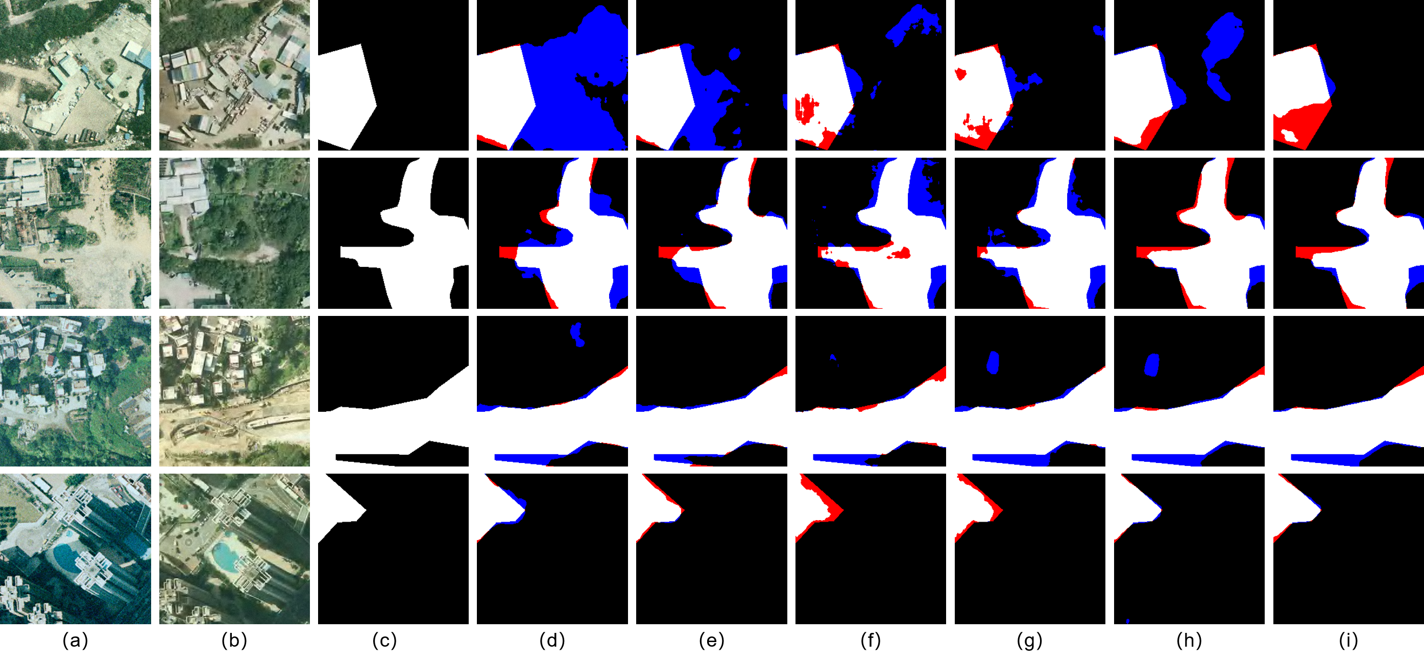
Figure 9: Visual comparison on the SYSU-CD dataset. Red denotes missed detections (FN). Blue indicates false alarms (FP). (a) Image at Time 1. (b) Image at Time 2. (c) Ground Truth. (d) Changer-MiT-b1 (Original). (e) Changer-MiT-b1 (MTKD). (f) CGNet (Original). (g) CGNet (MTKD). (h) TTP (Original). (i) TTP (MTKD).

TABLE V: Impact of Different Numbers of Teacher Models on O-P and MTKD Performance

Method	Strategy	No. of $\mathcal{M}_{T}$	mIOU	mAcc	mPrecision	mFscore
		3	75.29 (+0.44)	81.40 (-0.44)	87.06 (+0.97)	81.32 (+0.34)
	O-P	2	75.44 (+0.59)	81.96 (+0.12)	85.85 (-0.24)	81.51 (+0.53)
		3	75.35 (+0.50)	81.76 (-0.08)	87.18 (+1.09)	81.28 (+0.30)
Changer (MiT-b0)	MTKD	2	75.72 (+0.87)	82.30 (+0.46)	86.80 (+0.71)	81.66 (+0.68)
		3	75.42 (-0.52)	81.67 (-0.32)	87.13 (-0.61)	81.43 (-0.50)
	O-P	2	75.91 (-0.03)	82.11 (+0.12)	87.87 (+0.13)	81.97 (+0.04)
		3	76.15 (+0.21)	82.85 (+0.86)	86.98 (-0.76)	82.13 (+0.20)
Changer (MiT-b1)	MTKD	2	76.77 (+0.83)	83.38 (+1.39)	87.30 (-0.44)	82.66 (+0.73)
		3	72.95 (-0.42)	79.71 (-0.60)	85.50 (+0.17)	79.12 (-0.53)
	O-P	2	73.56 (+0.19)	80.76 (+0.45)	85.07 (-0.26)	79.92 (+0.27)
		3	73.82 (+0.45)	80.32 (+0.01)	86.33 (+1.00)	79.91 (+0.26)
CGNet	MTKD	2	73.78 (+0.41)	80.61 (+0.29)	85.67 (+0.34)	79.89 (+0.24)
		3	76.69 (+1.64)	83.48 (+3.24)	87.27 (-2.55)	82.52 (+1.76)
	O-P	2	76.65 (+1.60)	82.98 (+2.74)	87.39 (-2.43)	82.49 (+1.73)
		3	76.85 (+1.80)	82.99 (+2.75)	88.05 (-1.77)	82.56 (+1.80)
TTP	MTKD	2	76.31 (+1.26)	83.24 (+3.00)	86.81 (-3.01)	82.22 (+1.46)

V-F Robustness of MTKD

To verify the robustness of the MTKD framework, we conduct the following two sets of experiments:

Impact of Different Numbers of Teacher Models on MTKD Performance

In the previous subsection, we have demonstrated that the MTKD framework based on three teacher models can significantly improve the performance of various CD models. Therefore, we further explore the performance of MTKD with two teacher models. We set a threshold of $th=0.10$ to divide the dataset into small and large partitions and train the models $\mathcal{M}_{T_{S}}$ and $\mathcal{M}_{T_{L}}$ on these partitions, respectively. Subsequently, the student model $\mathcal{M}_{S}$ is trained using the MTKD framework. Except for the reduced number of teacher models, all other experimental settings remain unchanged. Using the original models as a baseline, Table V compares the metrics of models trained with the O-P strategy and the MTKD framework under different numbers of teacher models. The results indicate that two teacher models can still achieve significant performance improvements over the baseline. Notably, for Changer-MiT-b0 and Changer-MiT-b1, the two-teacher model setup yields even greater improvements compared to the three-teacher setup. For CGNet, the O-P strategy with two teachers achieves higher mIoU and mFscore, although the MTKD performance is lower in this case. For TTP, the performance of O-P and MTKD under the three teacher model still remains the strongest. These experiments validate the robustness of our methods in terms of the number of teachers. They also suggest that for some models, reducing the number of teachers can lead to comparable or even superior results while consuming fewer training resources.

Performance of MTKD on the SYSU-CD Dataset

We further validated the effectiveness of the MTKD framework on the SYSU-CD dataset. Transformer-based Changer-MiT-b1, CNN-based CGNet, and FM-based TTP models are selected. As shown in Table VI, after MTKD optimization, all the models achieve higher mIoU and mFscore values, with the most significant improvement on CGNet (mIoU increased by 0.46% and mFscore increased by 0.60%). However, the O-P strategy does not yield better results compared to the original models. The visual comparison is presented in Fig. 9, illustrating the detection results of these algorithms on four image pairs. Comparing the 4th and 5th columns, it is evident that MTKD significantly reduces the false alarm rate for Changer-MiT-b1. For example, in the 1st row, large areas of false detection are eliminated, and in the 3rd row, a small false-positive patch is removed. However, the 4th row exhibits an increase in false alarms. For CGNet, MTKD’s most notable contribution is the enhancement of internal compactness in detected regions. The original TTP model already produces satisfactory detection results, but MTKD further reduces false alarms. For instance, a large patch in the 1st row and a small patch in the 3rd row are effectively eliminated. However, the 1st row also shows an increase in missed detections. Overall, MTKD demonstrated substantial effectiveness on the SYSU-CD dataset, further validating its robustness.

TABLE VI: Experimental Results on SYSU-CD Test Set

Method	Strategy	mIoU	mAcc	mPrecision	mFscore
Changer (MiT-b1)	-	75.49	84.25	86.38	82.38
	O-P	75.32	83.88	85.86	82.19
	MTKD	75.56	83.97	87.33	82.40
CGNet	-	71.41	80.32	84.72	78.82
	O-P	69.85	80.05	82.39	77.40
	MTKD	71.87	81.74	84.05	79.42
TTP	-	76.09	84.59	87.08	82.72
	O-P	75.97	84.54	86.20	82.66
	MTKD	76.11	83.93	87.77	82.77

VI Conclusion

In this work, we introduce a new benchmark dataset, JL1-CD, which significantly complements existing CD datasets by offering sub-meter resolution, a wide range of change types, and a large dataset scale. We also propose the MTKD framework, which significantly enhances the performance of CD models on dual-temporal remote sensing images with different change areas, without increasing time and computational complexity during inference. Our approach effectively improves the generalization and robustness of the model across different cD scenarios. Future work will focus on developing a more universal knowledge distillation framework that not only further enhances model performance in diverse scenarios but also reduces model size and increases inference speed.

References

- [1] L. Wang, M. Zhang, X. Gao, and W. Shi, “Advances and challenges in deep learning-based change detection for remote sensing images: A review through various learning paradigms,” Remote Sensing, vol. 16, no. 5, p. 804, 2024.
- [2] P. R. Coppin and M. E. Bauer, “Digital change detection in forest ecosystems with remote sensing imagery,” Remote sensing reviews, vol. 13, no. 3-4, pp. 207–234, 1996.
- [3] R. D. Johnson and E. Kasischke, “Change vector analysis: A technique for the multispectral monitoring of land cover and condition,” International journal of remote sensing, vol. 19, no. 3, pp. 411–426, 1998.
- [4] G. Byrne, P. Crapper, and K. Mayo, “Monitoring land-cover change by principal component analysis of multitemporal landsat data,” Remote sensing of Environment, vol. 10, no. 3, pp. 175–184, 1980.
- [5] J. B. Collins and C. E. Woodcock, “An assessment of several linear change detection techniques for mapping forest mortality using multitemporal landsat tm data,” Remote sensing of Environment, vol. 56, no. 1, pp. 66–77, 1996.
- [6] A. A. Nielsen, K. Conradsen, and J. J. Simpson, “Multivariate alteration detection (mad) and maf postprocessing in multispectral, bitemporal image data: New approaches to change detection studies,” Remote Sensing of Environment, vol. 64, no. 1, pp. 1–19, 1998.
- [7] H. Nemmour and Y. Chibani, “Multiple support vector machines for land cover change detection: An application for mapping urban extensions,” ISPRS Journal of Photogrammetry and Remote Sensing, vol. 61, no. 2, pp. 125–133, 2006.
- [8] K. J. Wessels, F. Van den Bergh, D. P. Roy, B. P. Salmon, K. C. Steenkamp, B. MacAlister, D. Swanepoel, and D. Jewitt, “Rapid land cover map updates using change detection and robust random forest classifiers,” Remote sensing, vol. 8, no. 11, p. 888, 2016.
- [9] T. Celik, “Unsupervised change detection in satellite images using principal component analysis and -means clustering,” IEEE geoscience and remote sensing letters, vol. 6, no. 4, pp. 772–776, 2009.
- [10] R. C. Daudt, B. Le Saux, and A. Boulch, “Fully convolutional siamese networks for change detection,” in 2018 25th IEEE international conference on image processing (ICIP). IEEE, 2018, pp. 4063–4067.
- [11] C. Han, C. Wu, H. Guo, M. Hu, J. Li, and H. Chen, “Change guiding network: Incorporating change prior to guide change detection in remote sensing imagery,” IEEE Journal of Selected Topics in Applied Earth Observations and Remote Sensing, 2023.
- [12] Z. Liu, S. Wang, and Y. Gu, “A two-stage method for joint denoising and compression of sar images,” in 2024 IEEE 4th International Conference on Power, Electronics and Computer Applications (ICPECA). IEEE, 2024, pp. 853–859.
- [13] W. G. C. Bandara and V. M. Patel, “A transformer-based siamese network for change detection,” in IGARSS 2022-2022 IEEE International Geoscience and Remote Sensing Symposium. IEEE, 2022, pp. 207–210.
- [14] S. Fang, K. Li, and Z. Li, “Changer: Feature interaction is what you need for change detection,” IEEE Transactions on Geoscience and Remote Sensing, vol. 61, pp. 1–11, 2023.
- [15] Z. Liu, S. Wang, and Y. Gu, “Optimizing sar target detection through the multi-stage pre-training and fine-tuning strategy,” in 2024 IEEE 12th International Conference on Computer Science and Network Technology (ICCSNT). IEEE, 2024, pp. 178–181.
- [16] A. Dosovitskiy, “An image is worth 16x16 words: Transformers for image recognition at scale,” arXiv preprint arXiv:2010.11929, 2020.
- [17] A. Kirillov, E. Mintun, N. Ravi, H. Mao, C. Rolland, L. Gustafson, T. Xiao, S. Whitehead, A. C. Berg, W.-Y. Lo et al., “Segment anything,” in Proceedings of the IEEE/CVF International Conference on Computer Vision, 2023, pp. 4015–4026.
- [18] A. Radford, J. W. Kim, C. Hallacy, A. Ramesh, G. Goh, S. Agarwal, G. Sastry, A. Askell, P. Mishkin, J. Clark et al., “Learning transferable visual models from natural language supervision,” in International conference on machine learning. PMLR, 2021, pp. 8748–8763.
- [19] K. Li, X. Cao, and D. Meng, “A new learning paradigm for foundation model-based remote-sensing change detection,” IEEE Transactions on Geoscience and Remote Sensing, vol. 62, pp. 1–12, 2024.
- [20] S. Dong, L. Wang, B. Du, and X. Meng, “Changeclip: Remote sensing change detection with multimodal vision-language representation learning,” ISPRS Journal of Photogrammetry and Remote Sensing, vol. 208, pp. 53–69, 2024.
- [21] K. Chen, C. Liu, W. Li, Z. Liu, H. Chen, H. Zhang, Z. Zou, and Z. Shi, “Time travelling pixels: Bitemporal features integration with foundation model for remote sensing image change detection,” in IGARSS 2024-2024 IEEE International Geoscience and Remote Sensing Symposium. IEEE, 2024, pp. 8581–8584.
- [22] Z. Zheng, Y. Zhong, L. Zhang, and S. Ermon, “Segment any change,” arXiv preprint arXiv:2402.01188, 2024.
- [23] Z. Zhang, X. Jiang, Y. Zhou, and X. Liu, “Semi-supervised change detection with fourier-based frequency transformation,” IEEE Journal of Selected Topics in Applied Earth Observations and Remote Sensing, 2024.
- [24] G. Xu, Z. Zhang, X. Jiang, Y. Zhou, and X. Liu, “Semi-supervised scene classification for optical remote sensing images via label and embedding consistency,” IEEE Geoscience and Remote Sensing Letters, 2024.
- [25] K. Li, X. Cao, Y. Deng, J. Song, J. Liu, D. Meng, and Z. Wang, “Semicd-vl: Visual-language model guidance makes better semi-supervised change detector,” IEEE Transactions on Geoscience and Remote Sensing, 2024.
- [26] M. Gong, Y. Cao, and Q. Wu, “A neighborhood-based ratio approach for change detection in sar images,” IEEE Geoscience and Remote Sensing Letters, vol. 9, no. 2, pp. 307–311, 2011.
- [27] N. Otsu et al., “A threshold selection method from gray-level histograms,” Automatica, vol. 11, no. 285-296, pp. 23–27, 1975.
- [28] G. M. Gandhi, S. Parthiban, N. Thummalu, and A. Christy, “Ndvi: Vegetation change detection using remote sensing and gis–a case study of vellore district,” Procedia computer science, vol. 57, pp. 1199–1210, 2015.
- [29] F. Bovolo, L. Bruzzone, and M. Marconcini, “A novel approach to unsupervised change detection based on a semisupervised svm and a similarity measure,” IEEE transactions on geoscience and remote sensing, vol. 46, no. 7, pp. 2070–2082, 2008.
- [30] K. J. Wessels, F. Van den Bergh, D. P. Roy, B. P. Salmon, K. C. Steenkamp, B. MacAlister, D. Swanepoel, and D. Jewitt, “Rapid land cover map updates using change detection and robust random forest classifiers,” Remote sensing, vol. 8, no. 11, p. 888, 2016.
- [31] C. Zhang, P. Yue, D. Tapete, L. Jiang, B. Shangguan, L. Huang, and G. Liu, “A deeply supervised image fusion network for change detection in high resolution bi-temporal remote sensing images,” ISPRS Journal of Photogrammetry and Remote Sensing, vol. 166, pp. 183–200, 2020.
- [32] H. Chen and Z. Shi, “A spatial-temporal attention-based method and a new dataset for remote sensing image change detection,” Remote Sensing, vol. 12, no. 10, p. 1662, 2020.
- [33] S. Fang, K. Li, J. Shao, and Z. Li, “Snunet-cd: A densely connected siamese network for change detection of vhr images,” IEEE Geoscience and Remote Sensing Letters, vol. 19, pp. 1–5, 2021.
- [34] Z. Zheng, A. Ma, L. Zhang, and Y. Zhong, “Change is everywhere: Single-temporal supervised object change detection in remote sensing imagery,” in Proceedings of the IEEE/CVF international conference on computer vision, 2021, pp. 15 193–15 202.
- [35] C. Han, C. Wu, H. Guo, M. Hu, and H. Chen, “Hanet: A hierarchical attention network for change detection with bitemporal very-high-resolution remote sensing images,” IEEE Journal of Selected Topics in Applied Earth Observations and Remote Sensing, vol. 16, pp. 3867–3878, 2023.
- [36] A. Codegoni, G. Lombardi, and A. Ferrari, “Tinycd: A (not so) deep learning model for change detection,” Neural Computing and Applications, vol. 35, no. 11, pp. 8471–8486, 2023.
- [37] Y. Xing, J. Jiang, J. Xiang, E. Yan, Y. Song, and D. Mo, “Lightcdnet: Lightweight change detection network based on vhr images,” IEEE Geoscience and Remote Sensing Letters, 2023.
- [38] H. Chen, Z. Qi, and Z. Shi, “Remote sensing image change detection with transformers,” IEEE Transactions on Geoscience and Remote Sensing, vol. 60, pp. 1–14, 2021.
- [39] K. Yang, G.-S. Xia, Z. Liu, B. Du, W. Yang, M. Pelillo, and L. Zhang, “Asymmetric siamese networks for semantic change detection in aerial images,” IEEE Transactions on Geoscience and Remote Sensing, vol. 60, pp. 1–18, 2021.
- [40] G. Hinton, “Distilling the knowledge in a neural network,” arXiv preprint arXiv:1503.02531, 2015.
- [41] Z. Liu, S. Wang, Y. Li, Y. Gu, and Q. Yu, “Dsrkd: Joint despecking and super-resolution of sar images via knowledge distillation,” IEEE Transactions on Geoscience and Remote Sensing, 2024.
- [42] Z. Liu, S. Wang, and Y. Gu, “Sar image compression with inherent denoising capability through knowledge distillation,” IEEE Geoscience and Remote Sensing Letters, 2024.
- [43] L. Yan, J. Yang, and J. Wang, “Domain knowledge-guided self-supervised change detection for remote sensing images,” IEEE Journal of Selected Topics in Applied Earth Observations and Remote Sensing, vol. 16, pp. 4167–4179, 2023.
- [44] B. Wang, Z. Jiang, W. Ma, X. Xu, P. Zhang, Y. Wu, and H. Yang, “Dual-dimension feature interaction for semantic change detection in remote sensing images,” IEEE Journal of Selected Topics in Applied Earth Observations and Remote Sensing, 2024.
- [45] G. Wang, N. Zhang, J. Wang, W. Liu, Y. Xie, and H. Chen, “Knowledge distillation-based lightweight change detection in high-resolution remote sensing imagery for on-board processing,” IEEE Journal of Selected Topics in Applied Earth Observations and Remote Sensing, 2024.
- [46] C. Benedek and T. Szirányi, “Change detection in optical aerial images by a multilayer conditional mixed markov model,” IEEE Transactions on Geoscience and Remote Sensing, vol. 47, no. 10, pp. 3416–3430, 2009.
- [47] S. Ji, S. Wei, and M. Lu, “Fully convolutional networks for multisource building extraction from an open aerial and satellite imagery data set,” IEEE Transactions on geoscience and remote sensing, vol. 57, no. 1, pp. 574–586, 2018.
- [48] L. Shen, Y. Lu, H. Chen, H. Wei, D. Xie, J. Yue, R. Chen, S. Lv, and B. Jiang, “S2looking: A satellite side-looking dataset for building change detection,” Remote Sensing, vol. 13, no. 24, p. 5094, 2021.
- [49] N. Bourdis, D. Marraud, and H. Sahbi, “Constrained optical flow for aerial image change detection,” in 2011 IEEE international geoscience and remote sensing symposium. IEEE, 2011, pp. 4176–4179.
- [50] Q. Shi, M. Liu, S. Li, X. Liu, F. Wang, and L. Zhang, “A deeply supervised attention metric-based network and an open aerial image dataset for remote sensing change detection,” IEEE transactions on geoscience and remote sensing, vol. 60, pp. 1–16, 2021.
- [51] Z. Zheng, Y. Zhong, J. Wang, and A. Ma, “Foreground-aware relation network for geospatial object segmentation in high spatial resolution remote sensing imagery,” in Proceedings of the IEEE/CVF conference on computer vision and pattern recognition, 2020, pp. 4096–4105.
- [52] T. Xiao, Y. Liu, B. Zhou, Y. Jiang, and J. Sun, “Unified perceptual parsing for scene understanding,” in Proceedings of the European conference on computer vision (ECCV), 2018, pp. 418–434.
- [53] M. Contributors, “MMSegmentation: Openmmlab semantic segmentation toolbox and benchmark,” https://github.com/open-mmlab/mmsegmentation, 2020.
- [54] Y. Zhou, X. Yang, G. Zhang, J. Wang, Y. Liu, L. Hou, X. Jiang, X. Liu, J. Yan, C. Lyu et al., “Mmrotate: A rotated object detection benchmark using pytorch,” in Proceedings of the 30th ACM International Conference on Multimedia, 2022, pp. 7331–7334.
- [55] K. Li, J. Jiang, A. Codegoni, C. Han, Y. Deng, K. Chen, Z. Zheng, H. Chen, Z. Zou, Z. Shi et al., “Open-cd: A comprehensive toolbox for change detection,” arXiv preprint arXiv:2407.15317, 2024.