Atomic Proximal Policy Optimization for Electric Robo-Taxi Dispatch and Charger Allocation

Abstract

Pioneering companies such as Waymo have deployed robo-taxi services in several U.S. cities. These robo-taxis are electric vehicles, and their operations require the joint optimization of ride matching, vehicle repositioning, and charging scheduling in a stochastic environment. We model the operations of the ride-hailing system with robo-taxis as a discrete-time, average reward Markov Decision Process with infinite horizon. As the fleet size grows, the dispatching is challenging as the set of system state and the fleet dispatching action set grow exponentially with the number of vehicles. To address this, we introduce a scalable deep reinforcement learning algorithm, called Atomic Proximal Policy Optimization (Atomic-PPO), that reduces the action space using atomic action decomposition. We evaluate our algorithm using real-world NYC for-hire vehicle data and we measure the performance using the long-run average reward achieved by the dispatching policy relative to a fluid-based reward upper bound. Our experiments demonstrate the superior performance of our Atomic-PPO compared to benchmarks. Furthermore, we conduct extensive numerical experiments to analyze the efficient allocation of charging facilities and assess the impact of vehicle range and charger speed on fleet performance.

1 Introduction

Robo-taxi services have been deployed in several U.S. cities, including San Francisco, Phoenix, and Los Angeles [1]. The efficient operations of robo-taxi fleets, comprised of electric vehicles, is challenged by the stochasticity and the spatiotemporal distribution of trip demand, as well as the scheduling of battery charging with limited charging infrastructure. Inefficient operations could render vehicles unavailable during high-demand periods, leading to decreased service quality, reliability issues, and revenue loss.

In this work, we model the robo-taxi fleet dispatch problem as a Markov decision process with discrete state and action space. The state of system records the spatial distribution of vehicles, their current tasks, active trip requests, and the availability of chargers. Based on the state, the system dispatches the entire fleet to manage trip fulfillment, repositioning, charging, and passing (i.e. continuing with their current tasks), resulting in associated rewards or costs. Our goal is to find a fleet dispatching policy that maximizes the long-run average reward over an infinite time horizon.

The challenge of computing the fleet dispatching policy arises from the high-dimensionality of the state and action space. Since the state space contains all possible distributions of the fleet and the action space contains all feasible fleet assignments, both the state space and the action space scale exponentially with the fleet size. We develop a scalable deep reinforcement learning (RL) algorithm, which we refer as atomic proximal policy optimization (Atomic-PPO). The efficiency of Atomic-PPO is accomplished by decomposing the dispatching of the entire fleet into the sequential assignment of atomic action (tasks such as trip fullfillment, reposition, charge or pass (no new assignment)) to individual vehicles, which we refers to as “atomic action decomposition". The dimension of the atomic action space equals to the number of feasible tasks that can be assigned to an individual vehicle. Hence, the atomic action decomposition reduces the action space from being exponential in fleet size to being a constant, significantly reducing the complexity of policy training. We integrate our atomic action decomposition into a state-of-art RL algorithm, PPO [2], which possesses the monotonic policy improvement guarantee and has proven to be effective in control optimization across various applications [3, 4, 5, 6, 7]. We approximate both the value function and the atomic action function in the PPO training using neural networks, and further reduces the dimension of state representation by clustering the vehicle battery levels and destination information of trip requests.

To obtain an upper bound of the optimality gap of our fleet dispatching policy, we derive an upper bound on the optimal long-run average reward using a fluid-based linear program (LP) (see Theorem 1). The fluid limit is attained as the fleet size approaches infinity, with both trip demand volume and the number of chargers scaling up proportionally to the fleet size. Moreover, we benchmark our fleet dispatching policy against two heuristics. One of the heuristics is derived by applying randomized rounding to the fractional solution obtained from the fluid-based LP. The second heuristic is the power-of-k dispatching policy rooted in the load-balancing literature [8, 9]. The power-of-k dispatching heuristic selects k closest vehicles for a trip request and matches the request with the vehicle that has the highest battery level [10]. Varma et al. demonstrates that under the assumption that all trip requests and charging facilities are uniformly distributed across the entire service area, the power-of-k dispatching policy can achieve the asymptotically optimal service level. We note that this assumption is restrictive and is not satisfied in our setting.

We evaluate the performance of our Atomic PPO algorithm using the NYC For-Hire Vehicle dataset [11] in Manhattan area with a fleet size of 300, which is comparable to the fleet size deployed in a city by Waymo [12].The fleet size is approximately 5% of the for-hire vehicles in Manhattan area and we scale down the trip demand accordingly. Furthermore, our simulation incorporates the nonlinear charging rate, time-varying charging, repositioning cost and trip reward.

In our baseline setting, we assume that there are abundant number of DC Fast chargers (75 kW) in all regions. Our Atomic-PPO beats both benchmarks in terms of total reward by a large margin. In particular, Atomic-PPO can achieve as high as 91% of fluid upper bound, while the power-of-k dispatching and the fluid policy can only achieve 71% and 43% of fluid upper bound respectively. Moreover, our Atomic-PPO can achieve a near-full utilization of fleet for trip fulfillment during rush hours, while both benchmark policies have a significant number of vehicles idling at all time steps. The training of our Atomic-PPO is very efficient, as it can be completed within 3 hours using 30 CPUs.

Additionally, we investigate the impact of charging facility allocation, vehicle range, and charger outlet rate on the long-run average reward. We find that the uniform allocation of chargers across all regions is inefficient, as it requires 30 chargers (10% of the fleet size) to attain comparable long-run average reward as with abundant chargers. On the other hand, by allocating chargers according to ridership patterns, we only need 15 chargers (5% of the fleet size) to obtain the comparable performance. Additionally, we find that deploying fast chargers is crucial for the reward maximization. A fast charger reduces the amount of time it takes to refill a certain amount of battery, which then reduces the opportunity cost incurred by charging. However, in our setting, we find that investing in vehicles with a longer range is not important as most trips are relatively short and longer range does not reduces the time cost of charging.

Related Literature.

The problem of optimal fleet dispatch has been extensively studied in the context of ride-hailing systems, with the majority focuses on gasoline vehicles (and thus no need for scheduling charging) and several recent works on EVs [10, 13, 14, 15, 16, 17, 18, 19, 20, 21, 22, 23, 24, 25, 26, 27, 28, 29, 30, 31, 32, 33, 34, 35, 36, 37, 38]. The methods adopted in these literature fall into one of the three main categories: (1) deterministic optimization method; (2) queueing-based analysis; and (3) deep reinforcement learning.

(1) Deterministic optimization. The first category of works models the ride hailing system as a deterministic system, where all future trip arrivals are known. In deterministic systems, the optimal fleet dispatch can be formulated as a linear program [14] or mixed integer programs (MIP) [16, 15, 19, 39, 20, 23, 26, 28, 30, 32, 34]. These methods cannot be applied to settings with uncertain trip demand.

(2) Queueing-Based Analysis. The second category of works models ride-hailing systems using queueing theory. Some studies adopt a closed queueing system approach [40, 41, 42, 43, 44], where drivers remain in the system indefinitely. Others utilize an open queueing system framework [10, 22, 45, 46, 47, 48], where drivers dynamically enter and exit the system. Notably, the majority assume time-homogeneity in the system, with exceptions such as [46, 47, 44, 48], which address time-varying dynamics. Most of this research focuses on developing fleet control policies that are optimal under specific conditions or when the system reaches a fluid limit. Although these policies demonstrate provable optimality as fleet sizes approach infinity, their performance can suffer from significant optimality gaps when fleet sizes are moderate. Our construction of a reward upper bound builds on the fluid-based analytical methods established in this body of work.

(3) Deep Reinforcement Learning. The third category of research uses deep reinforcement learning (RL) to train fleet dispatching policies in complex environments that incorporate both spatial and temporal demand uncertainty. For a comprehensive review of these studies, see the recent survey by [49]. Majority of studies in this category including ours model the ride-hailing system as a Markov Decision Process (MDP), where dispatch decisions are made for the entire fleet at discreet time steps. A few articles modeled the system as a semi-MDP, where decision making is triggered by trip arrival or a vehicle completing a task [18, 21, 50, 27].

Existing research has primarily focused on two frameworks: finite-horizon settings, where decisions are optimized over a limited time frame, and discounted infinite-horizon settings, which prioritize near-term rewards. In contrast, we propose an infinite-horizon model with a long-run average reward objective. Finite-horizon or discounted settings may be effective in certain scenarios, such as with conventional vehicles, where the system resets each midnight during periods of low demand. However, these approaches are less suitable for managing electric fleets. The fleet control policies trained under these settings do not account for rewards in the long-run and therefore could lead to battery depletion across the fleet. If a ride-hailing company lacks sufficient charging facilities to recharge the entire fleet overnight, then the fleet with depleted batteries will be unable to fulfill trip requests the following day. Therefore, we argue that incorporating both infinite-horizon and average reward objectives is essential for electric vehicle operations because these features enable operators to optimize for steady-state battery levels across the fleet.

A major challenge in training fleet dispatching policies is managing the high dimensionality of state and action spaces. Consequently, most studies focus on specific subproblems, such as ride matching, vehicle repositioning, or charging, rather than developing integrated frameworks that address all these components simultaneously. A few studies have attempted to address multiple aspects of this challenge, including [31, 33, 37, 18, 36]. Building on these efforts, our model provides a comprehensive approach that unifies ride matching, repositioning, and charging into a holistic fleet management solution.

To tackle the curse of dimensionality arising from the large fleet size, prior works adopted various strategies that include (i) T-step look ahead approach [51] that computes the optimal fleet dispatching actions in the first $T$ steps of the value iteration by solving a linear program, (ii) warm start approach [52] that initializes the fleet dispatching policy by imitation learning from mixed integer programs, (iii) restricting vehicles at the same region to take the same action [53, 54], or (iv) relaxing integral constraints and treating the fleet action as continuous variables [55, 56, 57, 36, 58, 59, 60, 61, 62]. However, T-step look ahead approach and warm start approach are still computationally challenging as they need to repeatedly solve large-scale linear programs or mixed integer programs. The remaining two approaches may incur errors that increase in the system’s complexity, especially with the integration of ride-matching, repositioning, and charging.

Another extensively studied method to reduce the dimensionality of the policy space is to use a decentralized reinforcement learning (RL) training approach [63, 64, 65, 66, 67, 68, 69, 70, 71, 72, 73, 74, 75, 24, 76, 77, 78, 79, 80, 81, 67, 82, 83, 84, 85, 86, 87, 88, 89, 25, 29, 31, 33, 37]. In this approach, vehicles are treated as homogeneous and uncooperative agents that independently choose their own optimal actions based on a shared Q-function. While the decentralized RL approach effectively reduces the policy dimension, the induced policy is theoretically suboptimal because it does not consider the impact of their action on the state transition and system reward collectively. Our Atomic PPO algorithm addresses this issue by introducing a coordinated sequential assignment of atomic actions that incorporates state transitions after each step. This approach reduces the action space while ensuring the algorithm still accounts for the impact of each vehicle’s action on the system state and learns the accumulated rewards from the dispatch actions of the entire fleet in each decision epoch.

Finally, our Atomic-PPO algorithm builds on our previous work [90], which addressed ride matching and vehicle repositioning for conventional vehicle fleets within a finite-horizon framework. In this study, we extend the framework by incorporating charging and adopting an infinite-horizon, long-run average reward objective. Consequently, our algorithm introduces a new state reduction scheme to address these added complexities. Additionally, we provide a theoretical upper bound on the optimal long-run average reward, serving as a benchmark for our fleet dispatching policy. Experimental results show that our algorithm achieves a reward within 10% of the theoretical upper bound while maintaining low training costs.

2 Model

2.1 The ride-hailing system

We consider a transportation network with $V$ service regions. In this network, a fleet of electric vehicles with size $N$ are operated by a central planner to serve passengers, who make trip requests from their origins $u\in V$ to their destinations $v\in V$. For each pair of $(u,v)\in V\times V$, we assume that the battery consumption for traveling from $u$ to $v$ is a constant $b_{uv}\in\mathbb{R}_{\geq 0}$. The electric vehicles are each equipped with a battery of size $B$, i.e. a fully charged vehicle can take trips with total battery consumption up to $B$. A set of chargers with different charging rates $\delta\in\Delta$ are installed in the network, where each rate $\delta$ charger can replenish $\delta$ amount of battery to the connected vehicle in one unit of time. We denote the number of rate $\delta\in\Delta$ chargers in each region $v\in V$ as $n_{v}^{\delta}\in\mathbb{N}_{\geq 0}$.

We model the operations of a ride-hailing system as a discrete-time, average reward Markov Decision Process (MDP) with infinite time horizon. In particular, we model the system as an infinite repetition of a single-day operations, where each day $d=1,2,\dots$ is evenly partitioned into $T$ number of time steps $t=1,\dots,T$. The system makes a dispatching decision for the entire fleet at every time steps of a day, which we refer to as a decision epochs. In each decision epoch $(t,d)$, the number of trip requests between each $u$-$v$ pair, denoted as $X_{uv}^{t,d}$, follows a Poisson distribution with mean $\lambda_{uv}^{t}$. The duration of trips from region $u$ to region $v$ at time $t$ is a constant $\tau_{uv}^{t}$ that is a multiple of the length of a time step. Both $\lambda_{uv}^{t}$ and $\tau_{uv}^{t}$ can vary across time steps in a single day, but remain unchanged across days.

When the central planner receives the trip requests, they assign vehicles to serve (all or a part of) the requests. In particular, a vehicle must be assigned to the passenger within the connection patience time $L_{c}\geq 0$, and a passenger will wait at most time $L_{p}\geq 0$ (defined as the pickup-patience time) for an assigned vehicle to arrive at their origin. Otherwise, the passenger will leave the system. Both $L_{p}$ and $L_{c}$ are multiples of the discrete time steps.

The central planner keeps track of the status of each vehicle by the region $v\in V$ it is currently located or heading to, remaining time to reach $\eta=0,\dots,\hat{\tau}_{v}$, and remaining battery level $b=0,\dots,B$ when reaching $v$. Here, $\hat{\tau}_{v}:=\max_{u\in V,t\in[T]}\tau_{uv}^{t}$ is the maximum duration of any trip with destination $v$. We assume that the minimum time cost of all trips $\min_{u,v\in V,t\in[T]}\tau_{uv}^{t}$ is larger than $L_{p}$ so that no vehicle can be assigned to serve more than one trip request in a single decision epoch.

A vehicle is associated with status $c=(v,\eta,b)$ if (1) it is routed to destination $v$, with remaining time $\eta$, and battery level $b$ at the arrival; or (2) it is being charged at region $v$, with remaining charging time $\eta$, and battery level $b$ after the charging period completes. Here, if $\eta=0$, then the vehicle is parked at region $v$. Additionally, if $\eta>0$, then the vehicle could either be taking a trip with a passenger whose destination is $v$, the vehicle is being repositioned to $v$, or the vehicle is being charged in $v$. Vehicle repositioning may serve two purposes: (1) to pick up the next passenger whose origin is $v$; (2) to be charged or idle at region $v$. We note that the maximum remaining time of a trip cannot exceed $\hat{\tau}_{v}+L_{p}$ since a vehicle is eligible to serve a passenger with destination $v$ if it can arrive at the origin of that trip within $L_{p}$ time and the maximum trip duration is $\hat{\tau}_{v}$. Moreover, a vehicle with status $(v,0,b)$ can be charged at region $v$ with rate $\delta$ if such a charger is available in $v$. After the vehicle is assigned to charge, it will remain charged for $J$ time steps. If the vehicle’s battery level is full or close to full, then it will charge to full and then idle for the remaining time of the charging period. We assume that $J>L_{p}$ so that vehicles assigned to charge will not be assigned to serve trip requests in the same decision epoch . Let $\mathcal{C}:=\left\{(v,\eta,b)\right\}_{v\in V,\eta=0,\dots,\hat{\tau}_{,}b=0,\dots,B}$ denote the set of all vehicle status.

A trip order is associated with status $o=(u,v,\xi)$ if it originates from $u$, heads to $v$, and has been waiting for vehicle assignment in the system for $\xi$ time steps. A trip with origin $u$ and destination $v$ can be served by a vehicle of status $(u,\eta,b)$ if (1) the vehicle can reach $u$ within the passenger’s pickup-patience time $L_{p}$ (i.e. $\eta\leq L_{p}$), and (2) the remaining battery of the vehicle when reaching $u$ is sufficient to complete the trip to $v$ (i.e. $b\geq b_{uv}$). We note that a vehicle may be assigned to pick up a new passenger before completing its current trip towards $u$ as long as it can arrive within $L_{p}$ time steps. We use $\mathcal{O}:=\left\{(u,v,\xi)\right\}_{u,v\in V,\ \xi=0,\dots,L_{c}}$ to denote the set of all trip status.

A charger is associated with st $w=(v,\delta,j)$ if it is located at region $v$ with a rate of $\delta$ and is $j$ time steps away from being available. Specifically, if $j=0$, the charger is available immediately. If $j>0$, the charger is currently in use and will take an additional $j$ time steps to complete the charging period. We use $\mathcal{W}:=\{(v,\delta,j)\}_{v\in V,\delta\in\Delta,j=0,\dots,J-1}$ to denote the set of all charger status. All notations introduced in this section are summarized in Table 1.

2.2 Markov decision process

We next describe the state, action, policy and reward of the Markov decision process (MDP).

State.

We denote the state space of the MDP as $\mathcal{S}$ with generic element $s$. The state vector $s^{t,d}$ records the time $t$ of day $d$, the trip order state $\left(s_{o}^{t,d}\right)_{o\in\mathcal{O}}$, the fleet state $\left(s_{c}^{t,d}\right)_{c\in\mathcal{C}}$, and the charger state $\left(s_{w}^{t,d}\right)_{w\in\mathcal{W}}$, where $s_{o}^{t,d}$ is the number of trip orders of status $o$, $s_{c}^{t,d}$ is the number of vehicles of status $c$, and $s_{w}^{t,d}$ is the number of chargers of status $w$ at $(t,d)$. For all $(t,d)$, the sum of vehicles of all status equals to the fleet size $N$. That is,

$$\sum_{c\in\mathcal{C}}s_{c}^{t,d}=N,\quad\forall t\in[T],\ d=1,2,\dots.$$ (1)

Additionally, the sum of chargers of all remaining charging times for each region $v$ and rate $\delta$ equals to the quantity of the corresponding charging facility $n_{v}^{\delta}$. That is, $\forall v\in V$ and $\forall\delta\in\Delta$,

$$\sum_{w:=(v,\delta,j)}s_{w}^{t,d}=n_{v}^{\delta},\quad\forall t\in[T],\ d=1,2,\dots.$$ (2)

Thus, the state vector is $s^{t,d}=\left(t,\left(s_{c}^{t,d}\right)_{c\in\mathcal{C}},\left(s_{o}^{t,d}\right)_{o\in\mathcal{O}},\left(s_{w}^{t,d}\right)_{w\in\mathcal{W}}\right)\in\mathcal{S}$. Here, we note that the number of new trip arrivals $X_{uv}^{t,d}$ can be unbounded. However, since the fleet size is $N$ and a trip order can be kept in the system for up to $L_{c}$ steps, the maximum number of trip orders arrived at one time step that can be served before being abandoned is $N(L_{c}+1)$. As a result, without loss of generality, we truncate the number of trip requests for each status entering the system during each decision epoch to $N(L_{c}+1)$, with any additional trip requests being rejected by the system. Hence, our state space $\mathcal{S}$ is finite.

Action.

We denote the action space of the MDP as $\mathcal{A}$ with generic element $a$. An action is a flow vector of the fleet that consists of the number of vehicles of each status assigned to take trips, reposition, charge, idle, and pass. We denote an action vector at time $t$ of day $d$ as $a^{t,d}:=\left(f^{t,d}_{c},e^{t,d}_{c},q^{t,d}_{c},i^{t,d}_{c},p^{t,d}_{c}\right)_{c\in\mathcal{C}}$, where:

• $f^{t,d}_{c}:=\left(f^{t,d}_{c,o}\in\mathbb{N}\right)_{o\in\mathcal{O}}$ determines the number of vehicles of each status $c$ assigned to fulfill each trip order status $o\in\mathcal{O}$ at time $t$ of day $d$. In particular, vehicles are eligible to take trip requests if their current location or destination matches the trip’s origin region, they are within $L_{p}$ time steps from completing the current task, and they have sufficient battery to complete the trip, i.e.

  $$f^{t,d}_{c,o}\left\{\begin{array}[]{ll}\geq 0,&\quad\text{$\forall c=(u,\eta,b)$ and $o=(u,v,\xi)$}\\ &\text{ such that $\eta\leq L_{p}$ and $b\geq b_{uv}$},\\ =0,&\quad\text{otherwise.}\end{array}\right.$$ (6)

  Additionally, we require that the total number of vehicles that fulfill the trip orders of status $o$ cannot exceed $s_{o}^{t,d}$, i.e.

  $$\sum_{c=(u,\eta,b)\in\mathcal{C}}f^{t,d}_{c,o}\leq s_{o}^{t,d},\quad\forall o=(u,v,\xi)\in\mathcal{O}.$$ (7)

• $e^{t,d}_{c}:=\left(e^{t,d}_{c,v}\in\mathbb{N}\right)_{v\in V}$ represents the number of vehicles of each status $c$ assigned to reposition to $v$ at time $t$ of day $d$. In particular, vehicles are eligible to reposition to a different region if they have already completed their current tasks and they have sufficient battery to complete the trip.

  $$e^{t,d}_{c,v}\left\{\begin{array}[]{ll}\geq 0,&\quad\text{$\forall c=(u,\eta,b)$ and $v\neq u$}\\ &\text{ such that $\eta=0$ and $b\geq b_{uv}$},\\ =0,&\quad\text{otherwise.}\end{array}\right.$$ (11)

• $q^{t,d}_{c}:=\left(q^{t,d}_{c,\delta}\in\mathbb{N}\right)_{\delta\in\Delta}$ represents the number of vehicles of status $c$ assigned to charge with rate $\delta$ at time $t$ of day $d$. In particular, vehicles are eligible to charge if they have already completed their current tasks.

  $$q^{t,d}_{c,\delta}\left\{\begin{array}[]{ll}\geq 0,&\quad\text{$\forall c=(u,\eta,b)$ and $\delta\in\Delta$}\\ &\text{ such that $\eta=0$},\\ =0,&\quad\text{otherwise.}\end{array}\right.$$ (15)

  Additionally, for each region $v$ and charging rate $\delta$, we require that the total number of vehicles of all status assigned to charge at region $v$ with rate $\delta$ cannot exceed the total number of available chargers:

  $$\sum_{c=(v,\eta,b)\in\mathcal{C}}q^{t,d}_{c,\delta}\leq s_{(v,\delta,0)}^{t,d},\quad\forall v\in V,\ \delta\in\Delta.$$ (16)

• $i^{t,d}_{c}\in\mathbb{N}$ represents the number vehicles of status $c$ assigned to idle at time $t$ of day $d$. In particular, vehicles are eligible to idle if they have already completed their current tasks.

  $$i^{t,d}_{c}\left\{\begin{array}[]{ll}\geq 0,&\quad\text{$\forall c=(u,\eta,b)$ such that $\eta=0$},\\ =0,&\quad\text{otherwise.}\end{array}\right.$$ (19)

• $p^{t,d}_{c}\in\mathbb{N}$ represents the number of vehicles of status $c$ not assigned with any new action at time $t$ of day $d$. In particular, vehicles are eligible for the pass action if they have not completed their tasks yet.

  $$p^{t,d}_{c}\left\{\begin{array}[]{ll}\geq 0,&\quad\text{$\forall c=(u,\eta,b)$ such that $\eta>0$},\\ =0,&\quad\text{otherwise.}\end{array}\right.$$ (22)

For any $t$ and $d$, the vector $a^{t,d}$ needs to satisfy the following flow conservation constraint: All vehicles of each status should be assigned to trip-fulfilling, repositioning, charging, idling, or passing actions. That is,

$$\sum_{o\in\mathcal{O}}f^{t,d}_{c,o}+\sum_{v\in V}e^{t,d}_{c,v}+\sum_{\delta\in\Delta}q^{t,d}_{c,\delta}+i^{t,d}_{c}+p^{t,d}_{c}=s_{c}^{t,d}$$

$$\qquad\forall c\in\mathcal{C},\ t\in[T],\ d=1,2,\dots.$$ (23)

From the above description, we note that the feasibility of an action depends on the state. We denote the set of actions that are feasible for state $s$ as $\mathcal{A}_{s}$.

Policy.

The policy $\pi:\mathcal{S}\rightarrow\Delta(\mathcal{A}_{s})$ is a randomized policy that maps the state vector to an action, where $\pi(a|s)$ is the probability of choosing action $a$ given state $s$ under policy $\pi$. We note that the notation $\pi(\cdot)$ does not explicitly depend on $t$ since $t$ is already a part of the state vector $s$.

State Transitions.

At any time $t$ of day $d$, given any state $s$ and the action $a\in\mathcal{A}_{s}$, we compute the vehicle state vector at time $t+1$. For each vehicle status $c:=(v,\eta,b)\in\mathcal{C}$,

$$s_{(v,\eta,b)}^{t+1,d}=\left(\sum_{u\in V}\sum_{c^{\prime}=(u,\eta^{\prime},b^{\prime})\in\mathcal{C}}\sum_{o=(u,v,\xi^{\prime})\in\mathcal{O}}\right.$$

$$\qquad\left.f^{t,d}_{c^{\prime},o}\mathds{1}(\eta^{\prime}+\tau_{uv}^{t}-1=\eta,\ b^{\prime}-b_{uv}=b)\right)$$ (i)

$$\qquad+\left(\sum_{u\in V}\sum_{c^{\prime}=(u,0,b^{\prime})\in\mathcal{C}}e^{t,d}_{c^{\prime},v}\cdot\right.$$

$$\qquad\left.\mathds{1}(\tau_{uv}^{t}-1=\eta,\ b^{\prime}-b_{uv}=b)\right)$$ (ii)

$$\qquad+\left[\left(\sum_{\delta\in\Delta}q^{t,d}_{(v,0,b-\delta J),\delta}\mathds{1}(\eta=J-1,b\geq\delta J)\right)+\right.$$

$$\qquad\left.\left(\sum_{b^{\prime}>b-\delta J}\sum_{\delta\in\Delta}q^{t,d}_{(v,0,b^{\prime}),\delta}\mathds{1}(\eta=J-1,b=B)\right)\right]$$ (iii)

$$\qquad+\underbrace{i^{t,d}_{(v,\eta,b)}\mathds{1}(\eta=0)}_{(iv)}+\underbrace{p^{t,d}_{(v,\eta+1,b)}\mathds{1}(\eta<\hat{\tau})}_{(v)},$$ (24)

where (i) and (ii) correspond to vehicles assigned to new trip-fulfilling or repositioning actions with destination $v$, respectively. The destination, time to arrival, and battery level of these vehicles are updated based on the newly assigned trips. Term (iii) corresponds to the vehicles assigned to charge at time $t$. The battery level of these vehicles will be increased by $\delta J$ at the end of the charging period. If the vehicle is charged to full, then it will remain idle for the rest of the charging period. Term (iv) corresponds to the idling vehicles, and (v) corresponds to the vehicles taking the passing action whose remaining time of completing the assigned action decreases by $1$ in the next time step.

Moreover, the trip state at time $t+1$ of day $d$ is given by (29). For each trip status, we subtract the number of trip orders that have been fulfilled at time $t$, and we increment the active time by $1$ for trip orders that are still in the system. We abandon the trip orders that have been active for more than $L_{c}$ time steps. Additionally, new trip orders arrive in the system and we set their active time in the system to be $0$. That is, for all $(u,v)\in V\times V$,

$$s_{(u,v,\xi)}^{t+1,d}=\left\{\begin{array}[]{ll}\min\left\{X_{uv}^{t,d},\ N(L_{c}+1)\right\},\\ \quad\text{if $\xi=0$},\\ s_{(u,v,\xi-1)}^{t,d}-\sum_{c\in\mathcal{C}}f^{t,d}_{c,(u,v,\xi-1)},\\ \quad\text{if $1\leq\xi\leq L_{c}$}.\end{array}\right.$$ (29)

As mentioned earlier in this section, we cap the number of new trip arrivals by $N(L_{c}+1)$ so that the state space is finite. Then, trips that are not fulfilled at time $t$ are queued to $t+1$. Thus, the number of trips that have been in the system for $\xi\geq 1$ at time $t+1$ equals to that with $\xi-1$ from time $t$ minus the ones that are assigned to a vehicle at time $t$.

Lastly, the charger state at time $t+1$ of day $d$ is given by (34). For each charger status $w:=(v,\delta,j)\in\mathcal{W}$: For all region $v\in V$ and for all charger outlet rates $\delta\in\Delta$,

$$s_{(v,\delta,j)}^{t+1,d}=\left\{\begin{array}[]{ll}\sum_{c=(v,0,b)\in\mathcal{C}}q^{t,d}_{c,\delta},&\text{if }j=J-1,\\ s_{(v,\delta,j+1)}^{t,d},&\text{if }0<j<J-1,\\ s_{(v,\delta,1)}^{t,d}+\left(s_{(v,\delta,0)}^{t,d}\right.\\ \left.-\sum_{c=(v,0,b)\in\mathcal{C}}q^{t,d}_{c,\delta}\right),&\text{if }j=0.\end{array}\right.$$ (34)

At time $t+1$, the number of chargers with status $(v,\delta,j)$ (i.e. occupied and remaining time is $j=J-1$) equals the total number of vehicles just assigned to charge at time $t$. Chargers already in use at time $t$ will have their remaining charging time $j$ decrease by 1 when the system transitions to time $t+1$. The number of chargers available (i.e. $j=0$) at time $t+1$ consists of (i) the chargers that have just completed their charging periods (i.e. $s_{(v,\delta,1)}^{t,d}$), and (ii) the chargers available at time $t$ minus the ones that are assigned to charge vehicles (i.e. $s_{(v,\delta,0)}^{t,d}-\sum_{c=(v,0,b)\in\mathcal{C}}q^{t,d}_{c,\delta}$).

Reward.

The reward of fulfilling a trip request from $u$ to $v$ at time $t$ is $r^{t}_{f,uv}\in\mathbb{R}_{\geq 0}$. We remark that if a trip request has been active in the system for some time, then the reward is determined by the time at which the trip request is picked up. The reward (cost) of re-routing between $u,v$ is $r^{t}_{e,uv}\in\mathbb{R}_{\leq 0}$. The reward (cost) for a vehicle to charge at time $t$ is $r^{t}_{q,\delta}\in\mathbb{R}_{\leq 0}$. Idling and passing actions incur no reward or cost. As a result, given the action $a^{t,d}$, the total reward at time $t$ of day $d$ is given by

$$r^{t}(a^{t,d})= \sum_{c\in\mathcal{C}}\sum_{(u,v)\in V\times V}\sum_{\xi=0}^{L_{c}}r^{t}_{f,uv}f^{t,d}_{c,(u,v,\xi)}$$

$$+ \sum_{c\in\mathcal{C}}\sum_{(u,v)\in V\times V}r^{t}_{e,uv}e^{t,d}_{c,v}+\sum_{c\in\mathcal{C}}\sum_{\delta\in\Delta}r^{t}_{q,\delta}q^{t,d}_{c,\delta}.$$ (35)

The long-run average daily reward of a policy $\pi$ given some initial state $s$ is as follows:

$$R(\pi|s):=\lim_{D\rightarrow\infty}\frac{1}{D}\mathbb{E}_{\pi}\left[\sum_{d=1}^{D}\sum_{t=1}^{T}r^{t}(a^{t,d})\Biggm{\lvert}s\right].$$ (36)

Since the state is finite and the state transition and policy are homogeneous across days, the limit defined above exists (see page 337 of [91]). Our goal is to find the optimal fleet control policy $\pi^{*}$ that maximizes the long-run average daily rewards given any initial state $s$:

$$R^{*}(s)=R(\pi^{*}|s)=\max_{\pi}R(\pi|s),\quad\forall s\in\mathcal{S}.$$ (37)

Symbol	Description
$V$	The set of all service regions
$N$	Fleet Size
$B$	Vehicle battery range
$\Delta$	Set of charging rates
$T$	Number of time steps of each single day
$\tau_{uv}^{t}$	Trip duration from $u$ to $v$ at time $t$
$b_{uv}$	Battery consumption for traveling from region $u$ to $v$
$n_{v}^{\delta}$	Number of chargers of rate $\delta$ at region $v$
$\lambda_{uv}^{t}$	Trip arrival rate from $u$ to $v$ at time $t$
$X_{uv}^{t,d}$	Number of trip requests from $u$ to $v$ at time $t$ of day $d$
$L_{p}$	Maximum pickup patience time
$L_{c}$	Maximum assignment patience time
$J$	Duration of a charging period
$\mathcal{C}$	The set of all vehicle statuses, with a generic vehicle status denoted as $c$
$\mathcal{O}$	The set of all trip statuses, with a generic trip status denoted as $o$
$\mathcal{W}$	The set of all charger statuses, with a generic charger status denoted as $w$
$s^{t,d}$	The state vector at time $t$ of day $d$
$a^{t,d}$	The fleet action vector at time $t$ of day $d$
$f^{t,d}_{c,o}$	The number of vehicles of the status $c$ assigned to fulfill trips of status $o$ at time $t$ of day $d$
$e^{t,d}_{c,v}$	The number of vehicles of the status $c$ assigned to reposition to region $v$ at time $t$ of day $d$
$q^{t,d}_{c,\delta}$	The number of vehicles of the status $c$ assigned to charge with rate $\delta$ at time $t$ of day $d$
$i^{t,d}_{c}$	The number of vehicles of the status $c$ assigned to idle at time $t$ of day $d$
$p^{t,d}_{c}$	The number of vehicles of the status $c$ assigned to pass at time $t$ of day $d$
$r^{t}(a)$	The reward given action $a$ at time $t$

Table 1: Notations for the electric robo-taxi system

3 Fleet Control Policy Reduction With Atomic Actions

One challenge of computing the optimal control policy lies in the size of the action space $|\mathcal{A}|$, which grows exponentially with the number of vehicles $N$ and vehicle statuses $|\mathcal{C}|$. As a result, the dimension of policy $\pi$ also grows exponentially with $N$ and $|\mathcal{C}|$. The focus of this section is to address this challenge by introducing a policy reduction scheme, which decomposes the dispatching of a fleet to sequential assignment of tasks to individual vehicles, where the task for each individual vehicle is referred as an “atomic action". We use the name “atomic action policy" because each atomic action only changes the status of a single vehicle. In particular, for any vehicle of a status $c\in\mathcal{C}$, an atomic action can be any one of the followings:

• $\hat{\mathrm{f}}_{o}$ represents fulfilling a trip of status $o\in\mathcal{O}$.

• $\hat{\mathrm{e}}_{v}$ represents repositioning to destination $v\in V$.

• $\hat{\mathrm{q}}_{\delta}$ represents charging with rate $\delta\in\Delta$ at its current region.

• $\hat{\mathrm{p}}$ represents idling or continuing with its previously assigned actions.

We use $\hat{\mathcal{A}}$ to denote the atomic action space that includes all of the above atomic actions, i.e. $\hat{a}\in\hat{\mathcal{A}}:=\left\{\left(\hat{\mathrm{f}}_{o}\right)_{o\in\mathcal{O}},\left(\hat{\mathrm{e}}_{v}\right)_{v\in V},\left(\hat{\mathrm{q}}_{\delta}\right)_{\delta\in\Delta},\hat{\mathrm{p}}\right\}$. The atomic action significantly reduces the dimension of the action function since $\hat{\mathcal{A}}$ does not scale with the fleet size or the number of vehicle statuses.

We now present the procedure of atomic action assignment. In each decision epoch $(t,d)$, vehicles are arbitrarily indexed from $1$ to $N$, and are sequentially selected. For a selected vehicle $n$, the atomic policy $\hat{\pi}:\mathcal{S}\times\mathcal{C}\rightarrow\Delta(\hat{\mathcal{A}})$ maps from the tuple of system state $s^{t,d}_{n}$ before $n$-th assignment and the selected vehicle’s status $c_{n}$ to a distribution of atomic actions. The system state $s^{t,d}_{n}$ transitions after every single vehicle assignment with $s_{1}^{t,d}=s^{t,d}$, and $s_{N}^{t,d}$ transitions to $s^{t+1,d}$ after assigning the last vehicle and trip arrival at time $t+1$ is realized.

The total reward for each decision epoch $(t,d)$ is the sum of all rewards generated from each atomic action assignment in $(t,d)$, where the reward generated by the atomic action $\hat{a}^{t,d}\in\hat{\mathcal{A}}$ is given by

$$r^{t}(\hat{a}^{t,d})= \sum_{o\in\mathcal{O}}r^{t}_{f,o}\mathds{1}\left\{\hat{a}^{t,d}=\hat{\mathrm{f}}_{o}\right\}$$

$$+ \sum_{(u,v)\in V\times V}r^{t}_{e,uv}\mathds{1}\left\{\hat{a}^{t,d}=\hat{\mathrm{e}}_{v}\right\}$$

$$+ \sum_{\delta\in\Delta}r^{t}_{q,\delta}\mathds{1}\left\{\hat{a}^{t,d}=\hat{\mathrm{q}}_{\delta}\right\}.$$

The long-run average reward given the atomic action policy $\hat{\pi}$ and the initial state $s\in\mathcal{S}$ is as follows:

$$R(\hat{\pi}|s)$$

$$= \lim_{D\rightarrow\infty}\frac{1}{D}\mathbb{E}_{\hat{\pi}}\left[\sum_{d=1}^{D}\sum_{t=1}^{T}\sum_{n=1}^{N}r^{t}(\hat{a}^{t,d}_{n})\Bigg{|}s\right],\quad\forall s\in\mathcal{S},$$

where $\hat{a}_{n}^{t,d}$ is the atomic actions generated by the atomic action policy in the $n$-th atomic step in decision epoch $(t,d)$. Given any initial state $s\in\mathcal{S}$, our goal is to find the optimal atomic action policy such that $\hat{\pi}^{*}=\mathrm{argmax}_{\hat{\pi}}R(\hat{\pi}|s)$.

Our atomic action policy can be viewed as a reduction of the original fleet dispatching policy in that any realized sequence of atomic actions corresponds to a feasible fleet dispatching action with the same reward of the decision epoch. This reduction makes the training of atomic action policy scalable because the output dimension of atomic action policy $\hat{\pi}^{t}$ equals to $|\hat{\mathcal{A}}|$, which is a constant regardless of the fleet size.

4 Deep Reinforcement Learning With Aggregated States

The adoption of atomic actions has significantly reduced the action dimension. However, the implementation of the MDP is still challenging due to the large state space, which scales significantly with the fleet size, number of regions, and battery discretization. In this section, we provide an efficient algorithm to train the fleet dispatching policy by incorporating our atomic action decomposition into PPO [2]. To tackle with the large state size, we use neural networks to approximate both the value function and the policy function, to be specified later. We also further reduce the state size in terms of battery discretization and the number of regions by using the following state reduction scheme:

Battery Level Clustering.

We map the state representation of all vehicle statuses into vehicle statuses with aggregated battery levels. We cluster the battery levels into 3 intervals, each of which denotes low battery level $b_{L}$, medium battery level $b_{M}$, and high battery level $b_{H}$, respectively. The cutoff points can be set based on charging rates and criticality of battery levels. It is also possible to cluster the battery levels differently. If computing resources allow, we can cluster the battery levels with finer granularity, e.g. into 10 levels instead of 3.

Trip Order Status Clustering.

In the state reduction scheme, trip orders are aggregated by recording only the number of requests originating from or arriving at each region, instead of tracking the number of trip requests for each origin-destination pair. The clustering of trip order statuses reduces the state dimension from $O(|V|^{2})$ to $O(|V|)$. While it loses some information about the trip distribution, in numerical experiments, we demonstrate that the vehicle dispatching policy trained using our state reduction scheme still achieves a very strong performance (see Section 6).

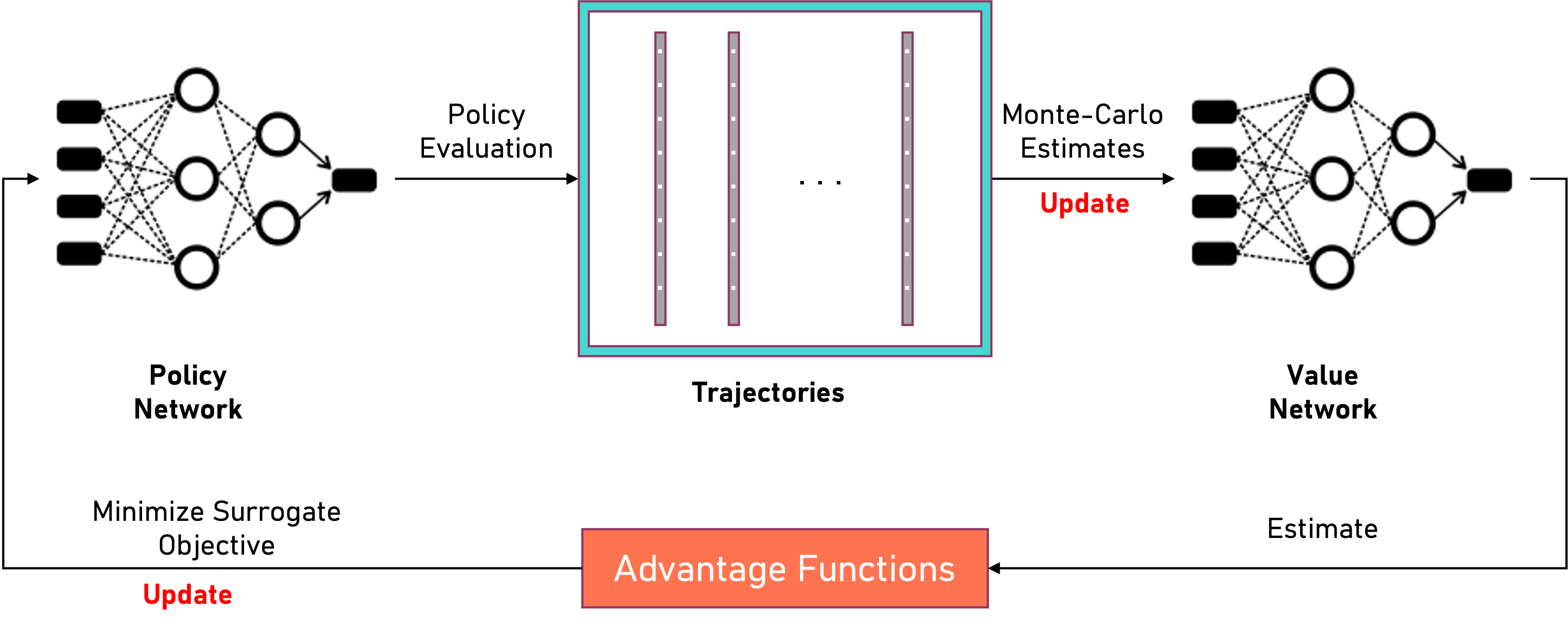
Figure 1: Atomic-PPO Training Pipeline

We denote the state space after the reduction on the original state as $\bar{\mathcal{S}}$, which we refer to as the “reduced state space". We use neural networks $\hat{\pi}_{\theta}:\bar{\mathcal{S}}\rightarrow\Delta(\hat{\mathcal{A}})$ on the reduced state space to approximate the atomic action policy function, where $\theta$ is the parameter vector for the atomic policy network.

Inputs: Number of policy iterations $M$, number of trajectories per policy iteration $K$, number of days per trajectory $D$, initial policy network $\hat{\pi}_{\theta_{0}}$

for policy iteration $m=1,\dots,M$ do

    Run policy $\hat{\pi}_{\theta_{m-1}}$ for $D$ days of $T$ time steps for $K$ trajectories of Monte-Carlo simulations and collect dataset (4).

    Construct empirical estimates of long-run average daily reward (39).

    Construct empirical estimates of relative value functions (4).

    Update relative value network by minimizing the mean-squared norm (42).

    Estimate advantage functions by (4).

    Obtain the updated policy network $\hat{\pi}_{\theta_{m}}$ by maximizing surrogate objective function (44).

end for

return policy $\hat{\pi}_{\theta_{M}}$

Algorithm 1 The Atomic-PPO Algorithm

Our Atomic-PPO algorithm (Figure 1) is formally presented in Algo. 1. For each policy iteration $m=1,\dots,M$, we maintain a copy of the policy neural network parameters $\theta_{m-1}$ from the previous iteration and hold it fixed throughout the iteration. Then, we generate a dataset $\mathrm{Data}^{(K)}_{\theta_{m-1}}$ by rolling out the atomic action policy $\hat{\pi}_{\theta_{m-1}}$ using $K$ trajectories of Monte Carlo simulation. This dataset includes the reduced state $\bar{s}^{t,d,(k)}_{n}$, atomic action $\hat{a}^{t,d,(k)}_{n}$, and atomic reward $r^{t}(\hat{a}^{t,d,(k)}_{n})$ at $n$-th atomic step of the decision epoch $(t,d)$ of trajectory $k$:

$$\mathrm{Data}^{(K)}_{\theta_{m-1}}:=$$

$$\left\{\left[\left[\left(\bar{s}^{t,d,(k)}_{n},\hat{a}^{t,d,(k)}_{n},r^{t}(\hat{a}^{t,d,(k)}_{n})\right)_{n=1}^{N}\right]_{t=1}^{T}\right]_{d=1}^{D}\right\}_{k=1}^{K},$$ (38)

In each trajectory, we truncate the roll-out to $D$ days, with $T$ time steps in each day. Here, we set $D$ to be a large number that exceeds the days for the system to be stationary given the policy, see Sec. 6 for more details. The procedure for the sequential assignment of atomic actions to individual vehicles follows from Section 3. Using the collected data, we construct the empirical estimate $\hat{g}$ of long-run average daily reward using(39).

$$\hat{g}=\frac{1}{KD}\sum_{k=1}^{K}\sum_{d=1}^{D}\sum_{t=1}^{T}\sum_{n=1}^{N}r^{t}(\hat{a}^{t,d,(k)}_{n}).$$ (39)

We also compute the empirical estimate of the relative value function of the current atomic policy $\hat{\pi}_{m-1}$. In particular, we define the relative value function $h_{n,m-1}$ of policy $\hat{\pi}_{m-1}$ at atomic step $n\in[N]$ as:

$$h_{n,m-1}(s)=\mathbb{E}_{\hat{\pi}_{\theta_{m-1}}}\left[\sum_{i=n}^{N}\left(r^{t}(\hat{a}^{t,d,(k)}_{i})-\frac{1}{TN}g_{m-1}\right)\right.$$

$$+\left.\sum_{\ell=t+1}^{T}\sum_{i=1}^{N}\left(r^{\ell}(\hat{a}^{\ell,d,(k)}_{i})-\frac{1}{TN}g_{m-1}\right)\Bigg{\lvert}s^{t,1}_{n}=s\right]$$

$$+\sum_{d=2}^{\infty}\sum_{\ell=1}^{T}\sum_{i=1}^{N}$$

$$\qquad\mathbb{E}_{\hat{\pi}_{\theta_{m-1}}}\left[\left(r^{\ell}(\hat{a}^{\ell,d^{\prime},(k)}_{i})-\frac{1}{TN}g_{m-1}\right)\Bigg{\lvert}s^{t,1}_{n}=s\right],$$

$$\qquad\qquad\forall s\in\mathcal{S},\ \forall t\in[T],$$ (40)

where $g_{m-1}$ is the long-run average daily reward achieved by $\hat{\pi}_{m-1}$ and we recall that the state $s$ contains the time of day $t$ information. By Proposition 2 in our concurrent work [92], the infinite series in (4) is well defined. Additionally, we remark that under the atomic action decomposition, our Markov chain has a period of $TN$, which is the total number of atomic steps in each day. Our definition of the relative value function is equivalent to the one defined using the Cesaro limit, as given by Puterman (see page 338 of [91]) for periodic chains, up to an additive constant (see Proposition 3 in [92]).

For any state $s^{t,d,(k)}_{n}$ in the atomic step $n$ of trajectory $k$ of decision epoch $(t,d)$, we construct an empirical estimate $\hat{h}^{t,d,(k)}_{n}$ of its relative value function as:

$$\hat{h}^{t,d,(k)}_{n}:=\sum_{i=n}^{N}\left(r^{t}(\hat{a}^{t,d,(k)}_{i})-\frac{1}{TN}\hat{g}\right)$$

$$\qquad+\sum_{\ell=t+1}^{T}\sum_{i=1}^{N}\left(r^{\ell}(\hat{a}^{\ell,d,(k)}_{i})-\frac{1}{TN}\hat{g}\right)$$

$$\qquad+\sum_{d^{\prime}=d+1}^{D}\sum_{\ell=1}^{T}\sum_{i=1}^{N}\left(r^{\ell}(\hat{a}^{\ell,d^{\prime},(k)}_{i})-\frac{1}{TN}\hat{g}\right).$$ (41)

Due to the large state space, we use neural networks $h_{\psi_{m-1}}:\bar{\mathcal{S}}\rightarrow\mathbb{R}$ on the reduced state space to approximate the relative value function for all atomic steps, where $\psi_{m-1}$ is the network parameters. We learn $h_{\psi_{m-1}}$ by minimizing the mean-square loss given the empirical estimates:

$$\sum_{k=1}^{K}\sum_{d=1}^{D}\sum_{t=1}^{T}\sum_{n=1}^{N}\left(h_{\psi_{m-1}}(\bar{s}^{t,d,(k)}_{n})-\hat{h}^{t,d,(k)}_{n}\right)^{2}.$$ (42)

This allows us to compute the empirical estimates of the advantage functions for each atomic step. The advantage function quantifies how much better (or worse) a specific atomic action $\hat{a}^{t,d,(k)}_{n}$ performs compared to following the previous stage policy $\hat{\pi}_{\theta_{m-1}}$ at a given reduced state $\bar{s}^{t,d,(k)}_{n}$.

$$\hat{A}_{\theta_{m-1}}(\bar{s}^{t,d,(k)}_{n},\hat{a}^{t,d,(k)}_{n}):=$$

$$\quad\begin{cases}r^{t}(\hat{a}^{t,d,(k)}_{n})-\frac{1}{TN}\hat{g}+\\ h_{\psi_{m-1}}(\bar{s}^{t,d,(k)}_{n+1})-h_{\psi_{m-1}}(\bar{s}^{t,d,(k)}_{n}),\\ \quad\text{if }n<N,\\ r^{t}(\hat{a}^{t,d,(k)}_{n})-\frac{1}{TN}\hat{g}+\\ h_{\psi_{m-1}}(\bar{s}^{t+1,d,(k)}_{1})-h_{\psi_{m-1}}(\bar{s}^{t,d,(k)}_{n}),\\ \quad\text{if }n=N,t<T,\\ r^{t}(\hat{a}^{t,d,(k)}_{n})-\frac{1}{TN}\hat{g}+\\ h_{\psi_{m-1}}(\bar{s}^{1,d+1,(k)}_{1})-h_{\psi_{m-1}}(\bar{s}^{t,d,(k)}_{n}),\\ \quad\text{if }n=N,t=T.\\ \end{cases}$$ (43)

Using the estimated advantage function $\hat{A}_{\theta_{m-1}}$, PPO algorithm select the the atomic action policy function of the next iteration $\hat{\pi}_{\theta_{m}}$ by choosing parameter $\theta_{m}$ that maximizes the clipped objective function defined as follows:

$$\hat{L}(\theta_{m},\theta_{m-1}):=\frac{1}{K}\sum_{k=1}^{K}\sum_{d=1}^{D}\sum_{t=1}^{T}\sum_{n=1}^{N}$$

$$\qquad\min\left(\frac{\hat{\pi}_{\theta_{m}}(\hat{a}^{t,d,(k)}_{n}|\bar{s}^{t,d,(k)}_{n})}{\hat{\pi}_{\theta_{m-1}}(\hat{a}^{t,d,(k)}_{n}|\bar{s}^{t,d,(k)}_{n})}\cdot\right.$$

$$\qquad\left.\hat{A}_{\theta_{m-1}}(\bar{s}^{t,d,(k)}_{n},\hat{a}^{t,d,(k)}_{n}),\right.$$

$$\qquad\left.\text{clip}\left(\frac{\hat{\pi}_{\theta_{m}}(\hat{a}^{t,d,(k)}_{n}|\bar{s}^{t,d,(k)}_{n})}{\hat{\pi}_{\theta_{m-1}}(\hat{a}^{t,d,(k)}_{n}|\bar{s}^{t,d,(k)}_{n})},1-\epsilon,1+\epsilon\right)\cdot\right.$$

$$\qquad\left.\hat{A}_{\theta_{m-1}}(\bar{s}^{t,d,(k)}_{n},\hat{a}^{t,d,(k)}_{n})\right),$$ (44)

where $\epsilon>0$ is a hyper parameter referred as the clip size of the training. The PPO policy update, as defined in (44), was introduced by [2] to enhance the computational efficiency of trust region policy optimization (TRPO) [93]. TRPO was developed to replace the original policy gradient method [94], offering the advantage of improved sample efficiency and the monotonic policy improvement guarantee.

5 Reward Upper Bound Provided By Fluid Approximation Model

Before presenting the performance of our atomic PPO algorithm, in this section, we construct an upper bound on the optimal long-run average reward using fluid limit. This upper bound will be used to construct an upper bound of optimality gap of our atomic PPO algorithm, as shown in the next section. We reformulate our robo-taxi dispatching problem as a fluid-based linear optimization program, where the fluid limit is attained as the fleet size approaches infinity, with both trip demand volume and the number of chargers scaling up proportionally to the fleet size. Under the fluid limit, the system becomes deterministic, and the fleet dispatching policy, which is a probability distribution of vehicle flows across all actions, reduces to a deterministic vector that represents the fraction of fleet assigned to each action at each time of the day.

We define the decision variables of the fluid-based optimization problem as follows:

1. Fraction of fleet for trip fulfilling $\bar{f}:=\left(\bar{f}^{t}_{c,o}\right)_{c\in\mathcal{C},o\in\mathcal{O},t\in[T]}$, where $\bar{f}^{t}_{c,o}$ is the fraction of vehicles with status $c$ fulfilling trip requests of status $o$ at time $t$.

2. Fraction of fleet for repositioning $\bar{e}:=\left(\bar{e}^{t}_{c,v}\right)_{c\in\mathcal{C},v\in V,t\in[T]}$, where $\bar{e}^{t}_{c,v}$ is the fraction of vehicles with status $c$ repositioning to $v$ at time $t$.

3. Fraction of fleet for charging $\bar{q}:=\left(\bar{q}^{t}_{c,\delta}\right)_{c\in\mathcal{C},\delta\in\Delta,t\in[T]}$, where $\bar{q}^{t}_{c,\delta}$ denotes the fraction of vehicles with status $c$ charging with rate $\delta$ at time $t$.

4. Fraction of fleet for continuing the current action $\bar{p}:=\left(\bar{p}^{t}_{c}\right)_{c\in\mathcal{C},t\in[T]}$, where $\bar{p}^{t}_{c}$ is the fraction of fleet with status $c$ taking the passing action at time $t$.

The fluid-based linear program aims at maximizing the total reward achieved by the fluid policy:

$$\max_{\bar{f},\bar{e},\bar{q},\bar{\mu},\bar{p}}N\sum_{t\in[T]}\sum_{c\in\mathcal{C}}\left\{\sum_{u\in V}\sum_{v\in V}\left[r^{t}_{f,uv}\sum_{\xi\in[L_{c}]}\bar{f}^{t}_{c,(u,v,\xi)}\right.\right.$$

$$\qquad+\left.\left.r^{t}_{e,uv}\bar{e}^{t}_{c,v}\right]+\sum_{\delta\in\Delta}r^{t}_{q,\delta}\bar{q}^{t}_{c,\delta}\right\},$$

$$\text{s.t.}\ \eqref{eq:fluid-ev-conservation-red}-\eqref{eq:fluid-nonneg-red}.$$

The constraints are given as follows:

1. The flow conservation for each vehicle status $c:=(v,\eta,b)\in\mathcal{C}$ at each time $t$ of a day.
   In particular, the left-hand side represents the vehicle flows from $t-1$ transitioning to the vehicle status $c$ according to (24). The right-hand side represents the assignment of vehicles of status $c$ to trip-fulfilling, repositioning, charging, and idling/passing actions.

   $$\left(\sum_{u\in V}\sum_{c^{\prime}=(u,\eta^{\prime},b^{\prime})\in\mathcal{C}}\sum_{o=(u,v,\xi^{\prime})\in\mathcal{O}}\right.$$

   $$\qquad\left.\bar{f}^{t-1}_{c^{\prime},o}\mathds{1}(\eta^{\prime}+\tau_{uv}^{t-1}-1=\eta,\ b^{\prime}-b_{uv}=b)\right)$$

   $$\qquad+\left(\sum_{u\in V}\sum_{c^{\prime}=(u,0,b^{\prime})\in\mathcal{C}}\bar{e}^{t-1}_{c^{\prime},v}\cdot\right.$$

   $$\qquad\left.\mathds{1}(\tau_{uv}^{t-1}-1=\eta,\ b^{\prime}-b_{uv}=b)\right)$$

   $$\qquad+\left[\left(\sum_{\delta\in\Delta}\bar{q}^{t-1}_{(v,0,b-\delta J),\delta}\mathds{1}(\eta=J-1,b\geq\delta J)\right)+\right.$$

   $$\qquad\left.\left(\sum_{b^{\prime}>b-\delta J}\sum_{\delta\in\Delta}\bar{q}^{t-1}_{(v,0,b^{\prime}),\delta}\mathds{1}(\eta=J-1,b=B)\right)\right]$$

   $$\qquad+\bar{p}^{t-1}_{(v,\eta,b)}\mathds{1}(\eta=0)+\bar{p}^{t-1}_{(v,\eta+1,b)}\mathds{1}(\eta<\hat{\tau})$$

   $$=\sum_{o\in\mathcal{O}}\bar{f}^{t}_{c,o}+\sum_{v\in V}\bar{e}^{t}_{c,v}+\sum_{\delta\in\Delta}\bar{q}^{t}_{c,\delta}+\bar{p}^{t}_{c},$$

   $$\qquad\forall c:=(v,\eta,b)\in\mathcal{C},\ t\in[T],$$ (45)

   We note that the time steps are periodic across days, and thus for $t=1$ in (45), $t-1$ is the last time step $T$ of the previous day. Similarly, in all of the subsequent constraints (46) – (47), the time step $t$ on the superscript of a variable being negative indicates time step $T-t$ in the previous day and $t>T$ indicates time step $t-T$ of the next day.

2. The fulfillment of trip orders does not exceed their arrivals.

   $$\sum_{c=(u,\eta,b)\in\mathcal{C}}\sum_{o=(u,v,\xi)\in\mathcal{O}}\bar{f}^{t+\xi}_{c,o}\leq\frac{1}{N}\lambda_{uv}^{t},$$

   $$\qquad\forall u,v\in V,\ t\in[T].$$ (46)

3. The number of vehicles charging at a specific rate in a given region does not exceed the corresponding charging capacity at any time.

   $$\sum_{j\in[J]}\sum_{c=(v,0,b)\in\mathcal{C}}\bar{q}^{t-j}_{c,\delta}\leq\frac{1}{N}n_{v}^{\delta},\forall\delta\in\Delta,\ t\in[T].$$ (47)

4. The battery is sufficient for vehicles to complete the trips for trip-fulfillment.

   $$\ \bar{f}^{t}_{c,o}\mathds{1}\{b<b_{uv}\}=0,$$

   $$\quad\forall c=(u,\eta,b)\in\mathcal{C},\ o=(u,v,\xi)\in\mathcal{O},\ t\in[T].$$ (48)

5. The battery is sufficient for vehicles to complete the trips for repositioning.

   $$\ \bar{e}^{t}_{c,v}\mathds{1}\{b<b_{uv}\}=0,$$

   $$\quad\forall c=(u,\eta,b)\in\mathcal{C},\ v\in V,\ t\in[T].$$ (49)

6. The fractions of vehicles of all statuses should add up to 1 at all times.

   $$\ \sum_{c\in\mathcal{C}}\left[\sum_{o\in\mathcal{O}}\bar{f}^{t}_{c,o}+\sum_{v\in V}\bar{e}^{t}_{c,v}+\sum_{\delta\in\Delta}\bar{q}^{t}_{c,\delta}+\bar{p}^{t}_{c}\right]=1,$$

   $$\qquad\qquad\qquad\qquad\qquad\qquad\forall t\in[T].$$ (50)

7. All decision variables are non-negative.

   $$\bar{f},\bar{e},\bar{q},\bar{p}\geq 0.$$ (51)

Let $\bar{R}$ be the optimal objective value from the fluid based LP.

Theorem 1.

$R^{*}(s)\leq\bar{R},\quad\forall s\in\mathcal{S}$.

The proof of Theorem 1 is deferred to the Appendix. Theorem 1 shows that $\bar{R}$ is an upper bound on the long-run average daily reward that can be achieved by any feasible policy. In the numerical section, we assess the gap between the average daily reward achieved by our Atomic-PPO and the fluid upper bound $\bar{R}$. This gap is an upper bound of optimality gap achieved by Atomic-PPO algorithm. We note that under the current formulation of the fluid-based LP, the number of variables scales with $|V|(L_{p}+\hat{\tau}{})BT$, where $\hat{\tau}{}$ can potentially be very large. We can reduce the size of this LP to $|V|L_{p}BT$ without loss of optimality by leveraging the fact that only vehicles with task remaining time $\eta<L_{p}$ can be assigned with new tasks, and therefore we only need to keep track of a fraction of fleet statuses when computing the optimal fluid policy. We delay the presentation of our simplified fluid-based LP to the appendix.

6 Numerical Experiments

We conduct numerical experiments using the for-hire vehicle trip records in July 2022 from New York City Taxi and Limousine Commission’s (TLC) [11]. The dataset contains the individual trip records of for-hire vehicles from Uber, Lyft, Yellow Cab, and Green Cab. Each trip record includes the origin and destination taxi zones, base passenger fares, trip duration, and distance, all of which are used for model calibration.

We consider trip requests from 0:00 to 24:00, Mondays to Thursdays , where each workday is partitioned into time intervals of 5 minutes. We estimate the mean of trip arrivals $\lambda_{uv}^{t}$ for each origin $u$ and destination $v$ at each time $t$ of a workday by taking the average of the number of trip requests of from $u$ to $v$ at time $t$. Ride-hailing trips in NYC show significant demand imbalances during morning (7-10 am) and evening (5-8 pm) rush hours, with zones experiencing more trips flowing in (red) or out (blue), as visualized in Figure 2.

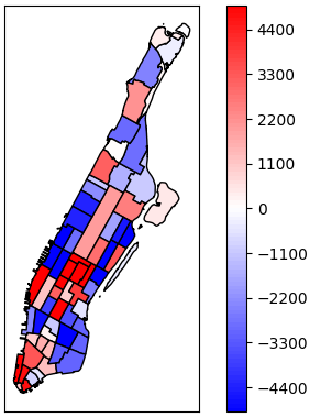
(a) Weekday Morning Rush Hours
7-10 am Mondays - Thursdays

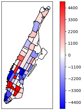
(b) Weekday Evening Rush Hours
5-8 pm Mondays - Thursdays

Figure 2: Manhattan Trip Demand Imbalance.

We partition the entire Manhattan into 10 regions (Figure 3) by aggregating adjacent taxi zones with similar demand patterns in both morning and evening rush hours. Based on the trip request pattern, we identify 3 categories of regions: workplace, restaurant area, and residential area. Workplaces are marked with red circles and mainly consist of downtown Manhattan and midtown Manhattan. Restaurants are mostly gathered in East Village and West Village circled in orange. Residential area consists of Upper/Midtown East, Upper/Midtown West, and upper Manhattan, and are circled in blue. During morning rush hours, people travel to workplaces (Figure 2(a)), while in the evening rush hours, they head to restaurants or residential areas (Figure 2(b)). Without repositioning, vehicles idle in high in-flow regions while abandoning trip requests in high out-flow regions. Therefore, it is critical to incorporate vehicle repositioning to balance the supply of vehicles across different regions in Manhattan.

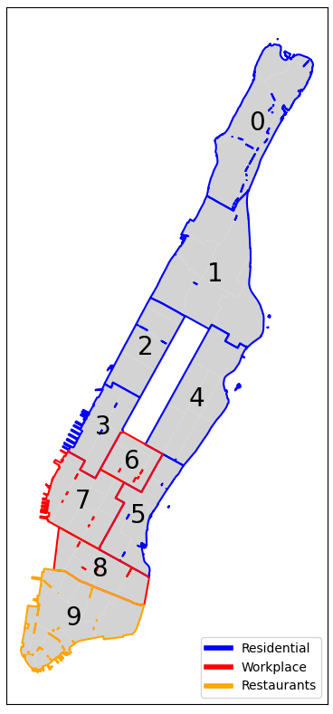
Figure 3: Service Regions in Manhattan.

Using the NYC TLC dataset, we build a simulator of trip order generating process. We set the environment parameter for numerical experiments according to Table 2. The reward of a trip $r^{t}_{f,uv}$ from region $u$ to $v$ at time $t$ is calibrated by taking the average of the base_passenger_fare column across all trips from $u$ to $v$ at time $t$. We estimate the actual fleet size using the maximum number of simultaneous trips across all times. Then, we scale down the mean of trip arrivals for all origin-destination pairs at all times based on the ratio of our chosen fleet size (i.e. 300) to the actual estimated fleet size (i.e. 12.8k).

We calibrate the battery consumption $b_{uv}$ for each origin $u$ and destination $v$ using the Chevrolet Bolt EUV model with battery pack size 65 kW. If fully charged, the range $B$ of the vehicle is 260 miles. For self-driving vehicles, this range is halved because the autonomous driving computation takes around 50% of the battery. We use 75 kW as the outlet rate of DC fast chargers and 15 kW for Level 2 AC (slow) chargers [95, 96].

We adopt the non-linear charging curve for charging (Table 3). Based on the criticality of battery level and the cutoff points of non-linear charging rates, we mark the battery level 0%-10% as “low", 10%-40% as “medium", and 40%-100% as “high" .

Parameter	Value
Decision Epoch Length	5 mins
Number of Time Steps Per Day	288
Number of Days Per Episode	8
Fleet Size	300
Battery Pack Size	65 kW
Vehicle Range	130 miles
Initial Vehicle Battery	Half Charged
Charger Outlet Rate	75 kW

Table 2: Environment parameters

Battery Percentage	0%-10%	10%-40%	40%-60%	60%-80%	80%-90%	90%-95%	95%-100%
Charging Time (s)	47	33	40	60	107	173	533

Table 3: Charging time (in sec) for each percentage increase in battery

We present the details about the architecture of neural networks and the hyperparameter settings for all experiments with Atomic-PPO (see Algorithm 1) in the Appendix A. For each experiment setting, we monitor the training logs of Atomic-PPO and terminate the training when the policy no longer makes improvements in the average reward across simulated trajectories. For most of the experiment settings, the training curve of Atomic-PPO converges after 10 policy iterations. In the evaluation phase, we roll out the Atomic-PPO policy on 10 consecutive days of operations for 10 different trajectories and compute the average daily reward. With 30 CPUs running the data generation (4) part of Atomic-PPO in parallel, each policy iteration takes 15-20 mins, so the entire training of Atomic-PPO on one problem instance takes 2-3 hours to complete.

We use the power-of-k dispatching and the fluid policy as our benchmark algorithms. For each trip request, the power-of-k heuristic selects the closest $k$ vehicles and assigns the one with the highest battery level to the trip request. If there are no vehicle that can reach the origin of the trip request within $L_{p}$ units of time, or if none of the $k$-closest vehicles have enough battery to complete the trip, then the trip request is abandoned. Upon completion of a trip, the vehicle will be routed to the nearest region with chargers. If, at the current decision epoch, the vehicle is not assigned any new trip requests and there is at least one charger unoccupied, then it will be plugged in at this charger and charge for one charging period. If all chargers are currently occupied or if the vehicle is fully-charged, then it will idle for the current decision epoch. The power-of-k dispatching policy is a very intuitive heuristic and is easy to implement. Under restrictive assumptions where all trip requests and charging facilities are uniformly distributed across the entire service area, [10] has demonstrated the effectiveness of power-of-k in achieving a high service level, which is the average fraction of trip demand served in the long-run. This assumption is not satisfied in our setting. We experiment $k=1,\dots,5$ and we set $k=2$ because it achieves the highest average reward.

For the fluid policy, we use the LP fluid solution to infer the number of vehicles deployed for each action, at each decision epoch $t$. We use randomized rounding to obtain a feasible policy from the LP fluid solution. The fluid policy is optimal under fluid limit, but not optimal when the fleet size is finite.

In Section 6.1, we demonstrate the effectiveness of our Atomic-PPO algorithm by comparing against the power-of-k dispatching algorithm and the fluid policy. In Section 6.2, we run our Atomic-PPO algorithm on multiple instances with different number of chargers and different locations of chargers. We draw insight on how the quantity and location of charging facility can impact the reward. For all experiments above, we use the DC fast chargers. In Section 6.3, we study how the vehicle range and outlets rate of chargers will affect the average reward achieved by the algorithm.

6.1 Experiments with Abundant Chargers

For experiments in this section, we assume that there are abundant chargers. In each region, the number of chargers equals to the fleet size (i.e. 300 chargers per region and 3000 chargers in total), so the chargers are available in all regions at all times under all policies.

Atomic-PPO achieves high percentage of fluid upper bound and significantly beats benchmark algorithms.

Table 4 shows the reward achieved by Atomic-PPO outperforms both of the fluid policy and the power-of-k by a large margin. After Atomic-PPO has been trained for 10 policy iterations, the average reward converges to around 91% of fluid upper bound. On the other hand, the power-of-k policy can achieve around 71% of fluid upper bound. The fluid policy has the worst performance and it achieves only 43% of the fluid upper bound.

Algorithm	Reward/$\bar{R}$	Avg. Daily Reward
Atomic-PPO	91%	$390K
Power of k	71%	$305K
Fluid policy	43%	$185K

Table 4: Reward achieved by Atomic-PPO and benchmarks

Atomic-PPO has a higher utilization of fleet for taking trip requests.

Figures 4(a)-4(c) demonstrate the fleet status of Atomic-PPO, power-of-k dispatching, and fluid policies respectively. Atomic-PPO has the largest fraction of passenger-carrying vehicles among all three policies across almost all time of the day, which illustrates that Atomic-PPO fulfills the highest number of trip requests. From 9 a.m. to 9 p.m., where the trip arrival rate is relatively higher than that of other hours, nearly all vehicles under Atomic-PPO are assigned to take trip requests.

However, a significant fraction of vehicles remain idle throughout the day under both the power-of-k heuristic and the fluid policy. The power-of-k heuristic does not allow for vehicle repositioning. When there are strong demand imbalance (Figure 2), the power-of-k heuristic cannot reposition vehicles from oversupply regions to pickup trip requests in undersupply regions. The fluid policy does not adapt to the stochasticity of the trip request arrivals as the policy is state-independent. When the number of trip arrivals $X_{uv}^{t}$ for a particular trip status is significantly larger than its Poisson arrival mean $\lambda_{uv}^{t}$, the fluid policy does not adjust its assignment to fulfill the additional trip requests.

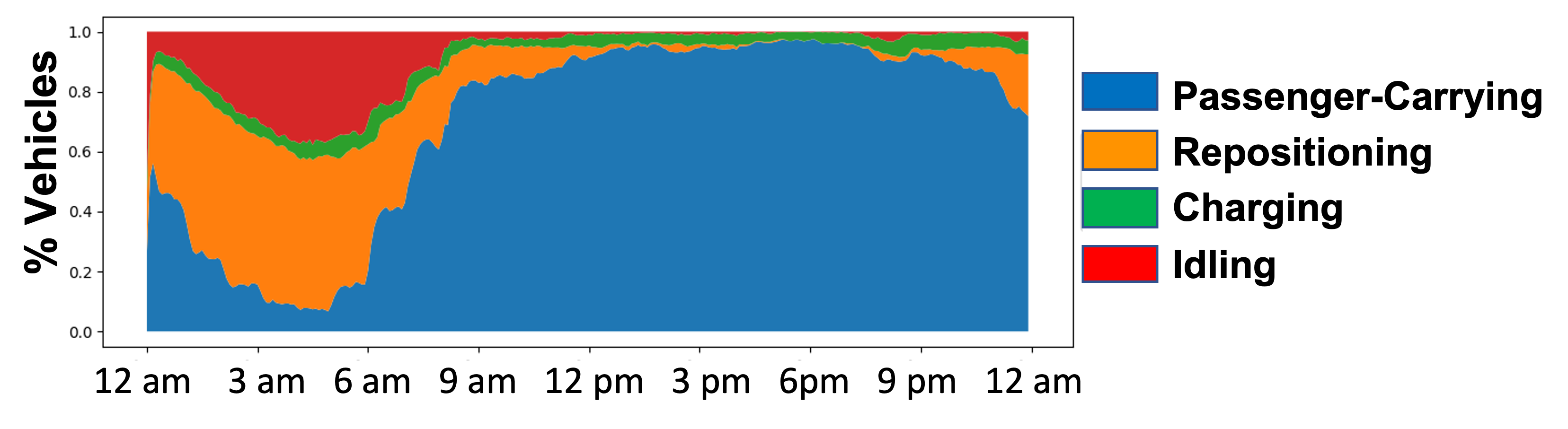
(a) Atomic-PPO

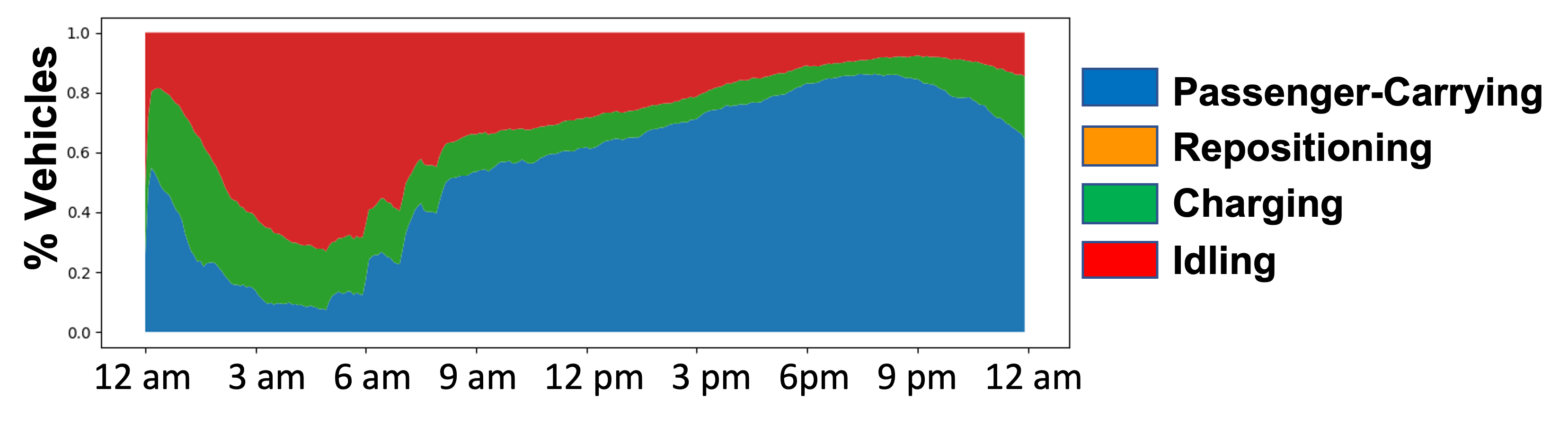
(b) Power of K

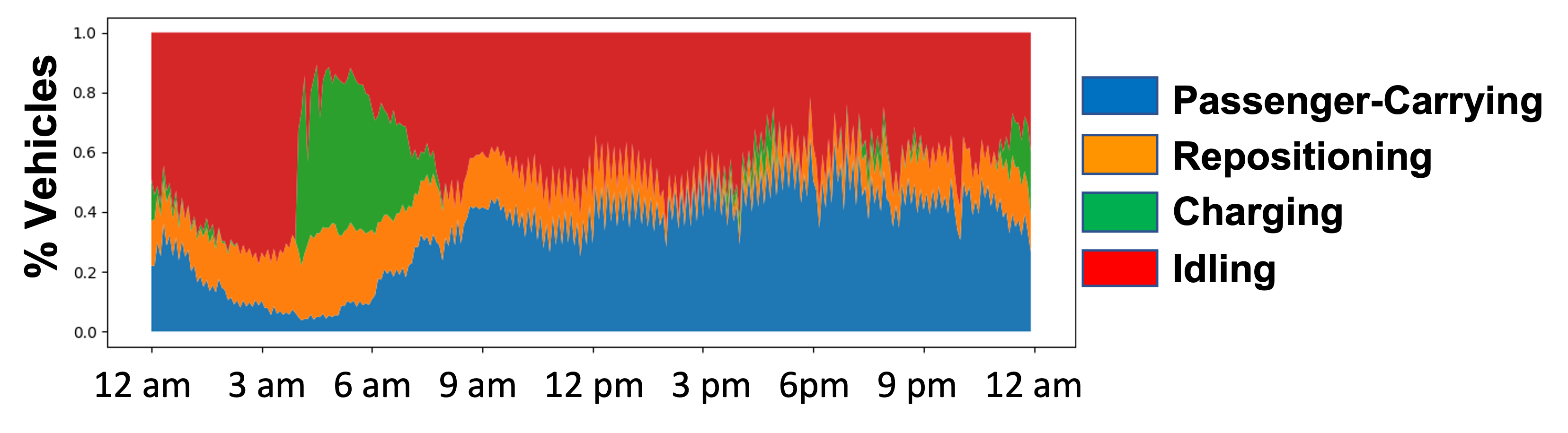
(c) Fluid Policy

Figure 4: Fleet status of Atomic-PPO, power-of-k, and fluid policy

Atomic-PPO has higher trip fulfillment across all times of a day.

Figures 5(a)-5(c) illustrate the trip fulfillment of Atomic-PPO, power-of-k, and fluid policies, respectively. Atomic-PPO fulfills a higher number of trip requests at all time steps of the day, compared to the power-of-k and fluid-policy. Note that the power-of-k policy can fulfill almost all trip requests during early morning hours (0-6 am) when the trip demand is small, but it fulfills significantly fewer trip requests than Atomic-PPO after 9 am when the trip demand is large. On the other hand, the fluid policy has the smallest number of fulfilled trip requests at all times of the day. It has to abandon some trip requests even during early morning hours, when the trip demand is small.

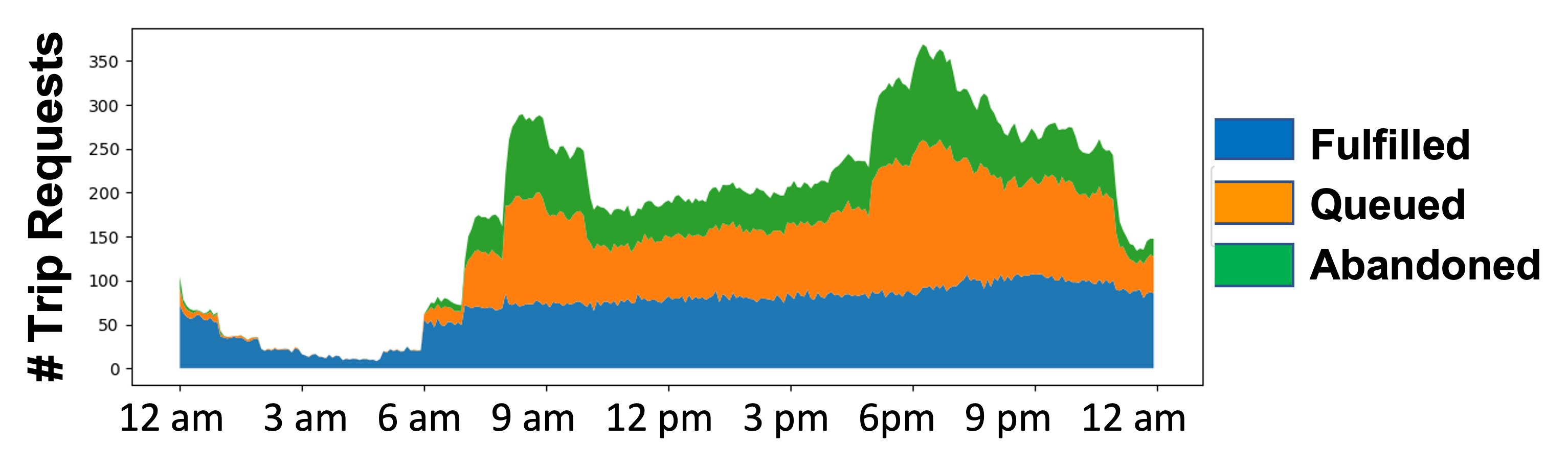
(a) Atomic-PPO

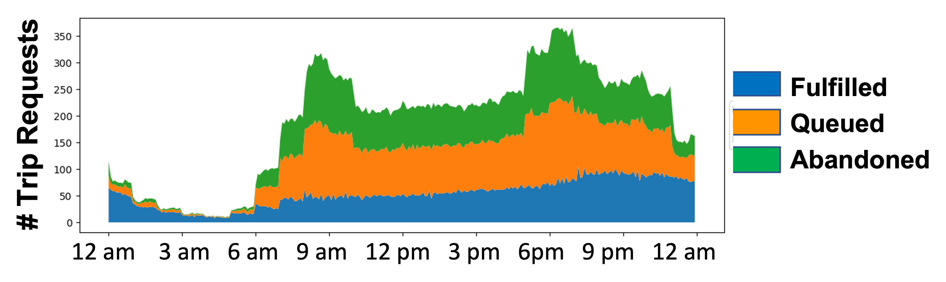
(b) Power of K

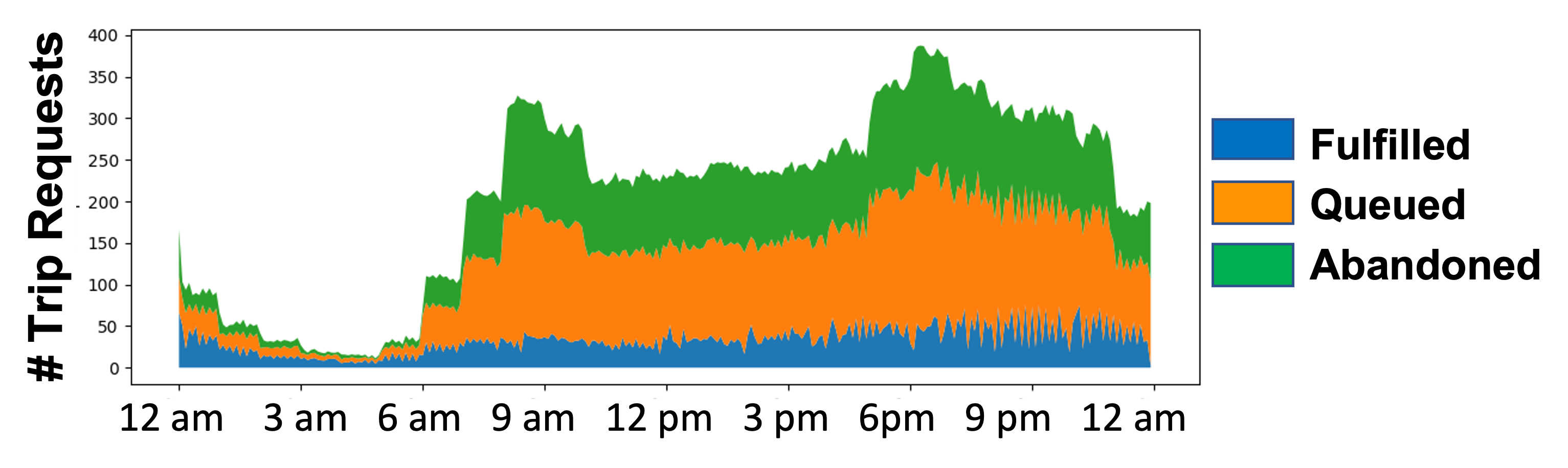
(c) Fluid Policy

Figure 5: Trip fulfillment status of Atomic-PPO, power-of-k, and fluid policy

6.2 Deployment of Charging Facilities

	Workplace					Restaurants	Residential
Region	0	1	2	3	4	5	6	7	8	9	Avg. Daily Reward
Unif. 10 chargers	1	1	1	1	1	1	1	1	1	1	$250K
Unif. 20 chargers	2	2	2	2	2	2	2	2	2	2	$375K
Unif. 30 chargers	3	3	3	3	3	3	3	3	3	3	$390K
Unif. 40 chargers	4	4	4	4	4	4	4	4	4	4	$390K
Midtown Manhattan.	0	0	0	15	0	0	0	0	0	0	$380K
Upper Manhattan	3	3	3	0	0	0	3	3	0	0	$225K
Lower Manhattan	0	0	0	0	3	3	0	0	3	3	$335K
Abundant Chargers	300	300	300	300	300	300	300	300	300	300	$390K
Fluid Upper Bound	300	300	300	300	300	300	300	300	300	300	$430K

Table 5: Deployment of Charging Facilities

We conduct experiments on different deployments of charging facilities. We first experiment with uniform deployment of chargers across the 10 regions and we run the Atomic-PPO training algorithm. Starting from 1 charger per region (i.e. 10 chargers in total), we keep increasing the number of chargers per region by 1, until the average reward reaches the level as that achieved by Atomic-PPO algorithm in the setting with abundant chargers as in Section 6.1. Additionally, we investigate the allocation of a limited number of chargers to a subset of regions. We allocate 15 chargers uniformly to all regions in lower Manhattan (regions 4, 5, 8, and 9), upper Manhattan (regions 0, 1, 2, 6, and 7), or midtown Manhattan (region 3). The average reward achieved by Atomic-PPO for each experiment case, along with the number of chargers per region, are summarized in Table 5.

Table 5 demonstrates that in order to achieve the same average reward as of the abundant chargers, we need 30 chargers if allocating them uniformly. Uniformly allocating 20 chargers leads to roughly 95% of reward generated by abundant chargers, and the performance degrades to roughly 65% when allocating uniformly with only 10 chargers. On the other hand, with only 15 chargers in total, it can achieve 88% reward of abundant chargers by allocating them uniformly to lower Manhattan, and it can achieve 98% reward of abundant chargers by allocating all to midtown Manhattan. Recall from Figure 2, midtown Manhattan region is the most popular destination during morning rush hours and it becomes the most popular origin during evening rush hours. Therefore, deploying all chargers in midtown reduces vehicles’ travel time to chargers, as vehicles can charge in midtown after finishing the morning rush-hour trips and before the evening rush-hour trips.

6.3 Vehicle Range and Charger Outlet Rates

In Table 6, we record average reward of experiments where all chargers are slow (15 kW) or all vehicles have doubled the range.

The deployment of fast chargers can effectively lead to an increase in reward, while doubling the vehicle range cannot.

Table 6 demonstrates that replacing fast chargers with slow chargers leads to 14% reduction in average daily reward, while doubling the vehicle range has little impact on reward. The reason is that when a vehicle is charging, it incurs an opportunity cost as the vehicle cannot take trip requests. Fast chargers enable vehicles to recharge more quickly than slow chargers, thereby reducing their opportunity cost. In contrast, doubling the vehicle range does not reduce the charging time required to replenish the same amount of battery, and thus it does not lower the opportunity cost. Moreover, the range does not have a significant impact for trips in Manhattan because most trips have a short distance.

Regime	Charger Outlet Rates	Vehicle Range	Avg. Daily Reward
Benchmark	75 kW	130 miles	$390K
Slow Chargers	15 kW	130 miles	$335K
Double Range	75 kW	260 miles	$390K

Table 6: Charging Rate & Vehicle Range

7 Concluding Remarks

In this article, we propose a scalable deep reinforcement learning algorithm, Atomic-PPO, to optimize the long-run average reward of a ride-hailing system with a robo-taxi fleet. In Atomic-PPO, we integrate our atomic action decomposition and state reduction into PPO, which is a state-of-art RL algorithm. Our atomic action decomposition reduces the action space from being exponential in fleet size to a constant, which significantly reduces the complexity of policy training. Moreover, our state reduction largely decreases the neural network input dimension, reducing the runtime and memory usage of our algorithm. We test our approach with extensive numerical experiments using the NYC for-hire vehicle dataset, where our algorithm significantly outperforms benchmarks in reward maximization. Additionally, we examine the impact of charger allocation, vehicle range, and charger outlet rates on reward. Our findings suggest that allocating chargers based on ridership patterns is more effective than a uniform distribution across regions. We also demonstrate that investing in fast chargers is crucial, while expanding vehicle range is less essential. For future research, we plan to extend Atomic-PPO to broader vehicle routing applications, such as delivery and logistics.

Appendix A Neural Network Parameters

We use deep neural networks to approximate the policy function and the value function. Both policy and value networks consist of a list of 3-layer shallow feed-forward networks corresponding to each of the decision epochs. The activation functions of the 3-layer shallow networks for the policy network are tanh, tanh, and tanh. The activation functions of the shallow networks for the value network are tanh, relu, and tanh.

We adopt a clipping with an exponential decay rate. Specifically, let $\epsilon$ be the initial clipping size, and $\gamma$ be the clipping decay factor, then at the policy iteration $m$, the clipping rate is $\max\{\epsilon\cdot\gamma^{m},0.01\}$. Table 7 specifies the hyperparameters for policy network and value network.

The policy and value networks are trained using the Adam solver. In each training epoch of a neural network, we randomly select a batch of training data and update the network parameters based on the gradient computed from this batch.

Hyperparameter	Value
Number of trajectories per policy iteration	30
Initial clipping size	0.1
Clipping decay factor	0.97
Learning rate for policy network	5e-4
Batch size for policy network	1024
Number of epochs for policy network	20
Learning rate for value network	3e-4
Batch size for value network	1024
Number of epochs for value network	100

Table 7: Hyperparameters for deep neural networks

Appendix B Fluid Based LP

B.1 Proof of Theorem 1

Proof.

Proof of Theorem 1 By theorem 9.1.8 in page 451 of [91], we know that there exists an optimal policy that is deterministic. Therefore, we only need to show that for any arbitrary deterministic stationary policy $\pi$, its long-run average daily reward $R(\pi|s)$ is upper bounded by the fluid-based LP optimal objective $\bar{R}$. Denote $(f(s^{t}),e(s^{t}),q(s^{t}),i(s^{t}),p(s^{t}))$ as a deterministic flow of vehicles generated by policy $\pi$ given state $s^{t}$ at time step $t$. Since the state space of the MDP is finite, we know that given any initial state $s\in\mathcal{S}$ and any deterministic stationary policy $\pi$, the system has a stationary state distribution, denoted as $\rho$. Here, the dependence of $\rho$ on the policy $\pi$ and the initial state $s$ is dropped for notation simplicity. By proposition 8.1.1 in page 333 of [91], the long-run average daily reward defined in (36) can be written as follows:

$$R(\pi|s)=\mathbb{E}_{\rho}\left[\sum_{t\in[T]}\sum_{c\in\mathcal{C}}\sum_{(u,v)\in V\times V}\right.$$

$$\qquad\ \left(r^{t}_{f,uv}\sum_{\xi\in[L_{c}]}f_{c,(u,v,\xi)}(s^{t})+r^{t}_{e,uv}e_{c,v}(s^{t})\right)$$

$$\quad+\left.\sum_{c\in\mathcal{C}}\sum_{\delta\in\Delta}r^{t}_{q,\delta}q_{c,\delta}(s^{t})\right].$$

Given $(f(s^{t}),e(s^{t}),q(s^{t}),i(s^{t}),p(s^{t}))$ for each state $s^{t}$ at each time step $t\in[T]$, we define the fleet dispatch fraction vector $(\bar{f}^{t},\bar{e}^{t},\bar{q}^{t},\bar{p}^{t})$ for each $t\in[T]$:

1. $\bar{f}^{t}_{c,o}:=\frac{1}{N}\mathbb{E}_{\rho}[f_{c,o}(s^{t})]$, $\forall c\in\mathcal{C}$, $o\in\mathcal{O}$, and $t\in[T]$,

2. $\bar{e}^{t}_{c,v}:=\frac{1}{N}\mathbb{E}_{\rho}[e_{(u,0,b),v}(s^{t})]$, $\forall c:=(u,0,b)\in\mathcal{C}$, $v\in V$, $v\neq u$, and $t\in[T]$,

3. $\bar{e}^{t}_{(v,0,b),v}:=\frac{1}{N}\mathbb{E}_{\rho}[i_{(v,0,b)}(s^{t})]$, $\forall c:=(v,0,b)\in\mathcal{C}$, $v\in V$, and $t\in[T]$,

4. $\bar{q}^{t}_{c,\delta}:=\frac{1}{N}\mathbb{E}_{\rho}[q_{c,\delta}(s^{t})]$, $\forall c\in\mathcal{C}$, $\delta\in\Delta$, and $t\in[T]$,

5. $\bar{p}^{t}_{c}:=\frac{1}{N}\mathbb{E}_{\rho}[p_{c}(s^{t})]$, $\forall c\in\mathcal{C}$ and $t\in[T]$,

where the expectations are taken over the states $s^{t}$. First, given that $(f(s^{t}),e(s^{t}),q(s^{t}),i(s^{t}),p(s^{t}))$ is a feasible fleet flow that satisfies all constraints in Sec. 2, we want to show that $(\bar{f},\bar{e},\bar{q},\bar{p})$ is a feasible solution to the fluid-based LP.

First, we show that the constraint (45) holds. The left-hand side aggregates all vehicles from $t-1$ that transitions to status $c$, while the right-hand side aggregates vehicles of status $c$ assigned to take all actions at time $t$. Both sides equal to the fraction of vehicles with status $c$ at time $t$, and thus (45) holds.

Next, we show that the constraint (46) holds. By (29), we obtain that for any $u,v\in V$ and any $t\in[T]$,

$$0\stackrel{{\scriptstyle(a)}}{{\leq}} s_{(u,v,L_{c})}^{t}-\sum_{c\in\mathcal{C}}f_{c,(u,v,L_{c})}(s^{t})$$

$$\stackrel{{\scriptstyle(b)}}{{=}} s_{(u,v,L_{c}-1)}^{t-1}-\sum_{c\in\mathcal{C}}\left(f_{c,(u,v,L_{c})}(s^{t})+f_{c,(u,v,L_{c}-1)}(s^{t-1})\right)$$

$$= \dots$$

$$\stackrel{{\scriptstyle(c)}}{{=}} s_{(u,v,0)}^{t-L_{c}}-\sum_{c\in\mathcal{C}}\sum_{\xi\in[L_{c}]}f_{c,(u,v,L_{c}-\xi)}(s^{t-\xi})$$

$$\stackrel{{\scriptstyle(d)}}{{\leq}} X_{uv}^{t-L_{c}}-\sum_{c\in\mathcal{C}}\sum_{\xi\in[L_{c}]}f_{c,(u,v,L_{c}-\xi)}(s^{t-\xi}),$$

where (a) is due to the constraint (7); (b) and (c) are obtained by (29) under the condition that $1\leq\xi\leq L_{c}$; and (d) is because the trip state $s_{(u,v,0)}^{t-L_{c}}$ is upper bounded by $X_{uv}^{t-L_{c}}$ as in (29) for $\xi=0$. Thus, we obtain

$$X_{uv}^{t-L_{c}}\geq \sum_{c\in\mathcal{C}}\sum_{\xi\in[L_{c}]}f_{c,(u,v,L_{c}-\xi)}(s^{t-\xi})$$

$$= \sum_{b\in[B]}\sum_{\eta\in[L_{p}]}\sum_{\xi\in[L_{c}]}f_{(u,\eta,b),(u,v,L_{c}-\xi)}(s^{t-\xi}).$$

We shift $t$ to be $t+L_{c}$, then the above inequality can be re-written as follows:

$$\frac{1}{N}X_{uv}^{t}$$

$$\geq \frac{1}{N}\sum_{b\in[B]}\sum_{\eta\in[L_{p}]}\sum_{\xi\in[L_{c}]}f_{(u,\eta,b),(u,v,L_{c}-\xi)}(s^{t+L_{c}-\xi})$$

$$= \frac{1}{N}\sum_{b\in[B]}\sum_{\eta\in[L_{p}]}\sum_{\xi\in[L_{c}]}f_{(u,\eta,b),(u,v,\xi)}(s^{t+\xi}),$$

where the second equation is due to swapping $L_{c}-\xi$ as $\xi$. Taking expectation on both sides, we obtain

$$\frac{1}{N}\lambda_{uv}^{t}= \mathbb{E}_{\rho}\left[\frac{1}{N}X_{uv}^{t}(s^{t})\right]$$

$$\geq \frac{1}{N}\mathbb{E}_{\rho}\left[\sum_{b\in[B]}\sum_{\eta\in[L_{p}]}\sum_{\xi\in[L_{c}]}f_{(u,\eta,b),(u,v,\xi)}(s^{t+\xi})\right]$$

$$= \sum_{b\in[B]}\sum_{\eta\in[L_{p}]}\sum_{\xi\in[L_{c}]}\mathbb{E}_{\rho}\left[\frac{1}{N}f_{(u,\eta,b),(u,v,\xi)}(s^{t+\xi})\right]$$

$$= \sum_{c=(u,\eta,b)\in\mathcal{C}}\sum_{o=(u,v,\xi)\in\mathcal{O}}\bar{f}^{t+\xi}_{c,o}.$$

The constraint (47) holds because:

$$\sum_{j\in[J]}\sum_{c=(v,0,b)\in\mathcal{C}}\bar{q}^{t-j}_{c,\delta}$$

$$= \frac{1}{N}\mathbb{E}_{\rho}\left[\sum_{j\in[J]}\sum_{c=(v,0,b)\in\mathcal{C}}q_{c,\delta}(s^{t-j})\right]$$

$$\stackrel{{\scriptstyle(a)}}{{=}} \frac{1}{N}\sum_{j=0}^{J-1}s_{(u,\delta,J-1)}^{t-j}$$

$$\stackrel{{\scriptstyle(b)}}{{=}} \frac{1}{N}s_{(u,\delta,1)}^{t-1}+\frac{1}{N}\sum_{j=1}^{J-1}s_{(u,\delta,j)}^{t}$$

$$\stackrel{{\scriptstyle(c)}}{{\leq}} \frac{1}{N}s_{(u,\delta,0)}^{t}+\frac{1}{N}\sum_{j=1}^{J-1}s_{(u,\delta,j)}^{t}$$

$$\stackrel{{\scriptstyle(d)}}{{=}} \frac{1}{N}n_{v}^{\delta},$$

where (a) is obtained by the case of $j=J-1$ in (34); (b) is obtained by the case of $0<j<J-1$ in (34); (c) is obtained by the case of $j=0$ in (34) and the constraint in (16); and (d) is obtained by (2).

Constraints (48) and (49) can be obtained by the constraints (6) and (11) in Sec. 2. The constraint (50) holds due to (1). Finally, the constraint (51) holds because all fleet actions must be non-negative as defined in Sec. 2. Hence, we obtain that $(\bar{f}(s^{t}),\bar{e}(s^{t}),\bar{q}(s^{t}),\bar{p}(s^{t}))$ is a feasible solution to the fluid-based LP.

Therefore, we have

$$R(\pi|s)=\mathbb{E}_{\rho}\left[\sum_{t\in[T]}\sum_{c\in\mathcal{C}}\sum_{(u,v)\in V\times V}\right.$$

$$\qquad\ \left(r^{t}_{f,uv}\sum_{\xi\in[L_{c}]}f_{c,(u,v,\xi)}(s^{t})+r^{t}_{e,uv}e_{c,v}(s^{t})\right)$$

$$\quad+\left.\sum_{c\in\mathcal{C}}\sum_{\delta\in\Delta}r^{t}_{q,\delta}q_{c,\delta}(s^{t})\right]$$

$$\stackrel{{\scriptstyle(a)}}{{=}} \sum_{t\in[T]}\sum_{c\in\mathcal{C}}\sum_{(u,v)\in V\times V}$$

$$\qquad\ \left(r^{t}_{f,uv}\sum_{\xi\in[L_{c}]}\mathbb{E}_{\rho}\left[f_{c,(u,v,\xi)}(s^{t})\right]\right.$$

$$\quad+\left.r^{t}_{e,uv}\mathbb{E}_{\rho}\left[e_{c,v}(s^{t})\right]\right)$$

$$\quad+\sum_{c\in\mathcal{C}}\sum_{\delta\in\Delta}r^{t}_{q,\delta}\mathbb{E}_{\rho}\left[q_{c,\delta}(s^{t})\right]$$

$$\stackrel{{\scriptstyle(b)}}{{=}} N\cdot\left[\sum_{t\in[T]}\sum_{c\in\mathcal{C}}\sum_{(u,v)\in V\times V}\right.$$

$$\qquad\ \left(r^{t}_{f,uv}\sum_{\xi\in[L_{c}]}\bar{f}^{t}_{c,(u,v,\xi)}+r^{t}_{e,uv}\bar{e}^{t}_{c,v}\right)$$

$$\quad+\left.\sum_{c\in\mathcal{C}}\sum_{\delta\in\Delta}r^{t}_{q,\delta}\bar{q}^{t}_{c,\delta}\right]$$

$$\stackrel{{\scriptstyle(c)}}{{\leq}} \bar{R},$$

where (a) is obtained by the linearity of expectation, (b) is by plugging in (i)-(v) above, (c) is because $(\bar{f},\bar{e},\bar{\mu},\bar{q},\bar{p})$ is a feasible solution to the fluid-based LP. As a result, the associated reward function value is upper bounded by the optimal value $\bar{R}$. $\square$ ∎

B.2 A formulation with reduced number of variables

In this section, we provide a way to formulate the fluid-based optimization problem with a smaller number of decision variables and constraints. The reduction is achieved based on the fact that only vehicles with task remaining time $\eta\leq L_{p}$ can be assigned with new tasks, and therefore we only need to keep track of the statuses of vehicles with task remaining time $\eta\leq L_{p}$ in the optimization.

We define the variables of the simplified fluid-based optimization problem as follows:

1. Fraction of fleet with a vehicle status for trip fulfilling $\bar{f}^{\dagger}:=\left(\bar{f}^{\dagger t}_{uv,b,\eta}\right)_{u,v\in V,t\in[T],b\in[B],\eta\in[L_{p}]}$, where $\bar{f}^{\dagger t}_{uv,b,\eta}$ is the fraction of vehicles with battery level $b$ at time $t$ that pick up trip requests from $u$ to $v$ with remaining waiting time $\eta$. We remark two differences of $\bar{f}^{\dagger}$ from the variable $\bar{f}$ in the original formulation: (i) $\bar{f}^{\dagger}$ only keeps track of the vehicles with task remaining time $\eta\leq L_{p}$, whereas $\bar{f}$ keeps track of vehicles of all statuses; (ii) $\bar{f}^{\dagger}$ can be considered as an aggregation of $\bar{f}$ across all trip active times $\xi$, i.e., $\bar{f}^{\dagger t}_{uv,b,\eta}=\sum_{\xi\in[L_{c}]}\bar{f}^{t}_{(u,\eta,b),(u,v,\xi)}$.

2. Fraction of fleet fulfilling trip requests with a certain status $\bar{\mu}^{\dagger}:=\left(\bar{\mu}^{\dagger t}_{uv,\eta,\xi}\right)_{u,v\in V,\eta\in[L_{p}],\xi\in[L_{c}],t\in[T]}$, where $\bar{\mu}^{\dagger t}_{uv,\eta,\xi}$ is fraction of vehicles assigned at time $t$ to a trip with o-d pair $uv$ that has been waiting for assignment for $\xi$ steps and will be pick up after $\eta$ time steps. We note that $\bar{\mu}^{\dagger}$ differs from $\bar{f}^{\dagger}$ in that $\bar{\mu}^{\dagger}$ aggregates the trip-fulfilling vehicles across battery level $b$, while $\bar{f}^{\dagger}$ aggregates them across trip active time $\xi$. In particular, $\bar{\mu}^{t}_{uv,\eta,\xi}=\sum_{b\in[B]}\bar{f}^{t}_{(u,\eta,b),(u,v,\xi)}$.

3. Fraction of fleet for repositioning $\bar{e}^{\dagger}:=\left(\bar{e}^{\dagger t}_{uv,b}\right)_{u,v\in V,t\in[T],b\in[B]}$, where $\bar{e}^{\dagger t}_{uv,b}$ is the fraction of vehicles with battery level $b$ at time $t$ repositioning from $u$ to $v$. Here, the variable $\bar{e}^{\dagger t}_{uv,b}$ is equivalent to the decision variable $\bar{e}^{t}_{(u,0,b),v}$ in the original formulation.

4. Fraction of fleet for charging $\bar{q}^{\dagger}:=\left(\bar{q}^{\dagger t}_{v,\delta,b}\right)_{v\in V,\delta\in\Delta,t\in[T],b\in[B]}$, where $\bar{q}^{\dagger t}_{v,\delta,b}$ denotes the fraction of vehicles with battery level $b$ charging at region $v$ with rate $\delta$ at time $t$. Here, the variable $\bar{q}^{\dagger t}_{v,\delta,b}$ is equivalent to the decision variable $\bar{q}^{t}_{(v,0,b),\delta}$ in the original formulation.

5. Fraction of fleet for continuing the current action $\bar{p}^{\dagger}:=\left(\bar{p}^{\dagger t}_{v,b,\eta}\right)_{v\in V,b\in[B],\eta\in[L_{p}],t\in[T]}$, where $\bar{p}^{\dagger t}_{v,b,\eta}$ is the fraction of fleet $\eta$ steps away with destination $v$ with battery $b$ that takes the passing action at time $t$. Here, the variable $\bar{p}^{\dagger t}_{v,b,\eta}$ is equivalent to the decision variable $\bar{p}^{t}_{(v,\eta,b)}$ in the original formulation. Again, we note that $\bar{p}^{\dagger}$ only keeps track of the vehicles statuses with task remaining time $\eta\leq L_{p}$, while $\bar{p}$ in the original formulation keeps track of all vehicle statuses.

The simplified fluid-based linear program is given as follows:

$$\max_{\bar{f}^{\dagger},\bar{e}^{\dagger},\bar{q}^{\dagger},\bar{\mu}^{\dagger},\bar{p}^{\dagger}}\ \ N\sum_{t\in[T]}\left\{\sum_{u\in V}\sum_{v\in V}\left[r^{t}_{f,uv}\right.\right.$$

$$\qquad\left.\left(\sum_{\xi\in[L_{c}]}\sum_{\eta\in[L_{p}]}\bar{\mu}^{\dagger t}_{uv,\eta,\xi}\right)+r^{t}_{e,uv}\sum_{b\in[B]}\bar{e}^{\dagger t}_{uv,b}\right]$$

$$\qquad+\left.\sum_{\delta\in\Delta}r^{t}_{q,\delta}\sum_{v\in V}\sum_{b\in[B]}\bar{q}^{\dagger t}_{v,\delta,b}\right\},$$

$$\text{s.t.}\ \left[\sum_{v\in V}\left(\sum_{\eta^{\prime}\in[L_{p}]}\bar{f}^{\dagger\phi_{vu}(t,\eta^{\prime})}_{vu,b+b_{vu},\eta^{\prime}}\right.\right.$$

$$\qquad+\left.\left.\bar{e}^{\dagger\phi_{vu}(t,0)}_{vu,b+b_{vu}}\mathds{1}\{v\neq u\}\right)\mathds{1}\{b+b_{vu}\leq B\}\right.$$

$$\qquad+\left.\sum_{\delta\in\Delta}\bar{q}^{\dagger(t+\eta-J)}_{u,\delta,b-\delta J}\mathds{1}\{b\geq\delta J\}\right.$$

$$\qquad+\left.\sum_{\delta\in\Delta}\sum_{b^{\prime}>B-\delta J}\bar{q}^{\dagger(t+\eta-J)}_{u,\delta,b^{\prime}}\mathds{1}\{b=B\}\right]\mathds{1}\{\eta=L_{p}\}$$

$$\qquad+\bar{e}^{\dagger(t-1)}_{uu,b}\mathds{1}\{\eta=0\}+\bar{p}^{\dagger(t-1)}_{u,b,\eta+1}\mathds{1}\{\eta<L_{p}\}$$

$$\quad=\sum_{v\in V}\left(\bar{f}^{\dagger t}_{uv,b,\eta}+\bar{e}^{\dagger t}_{uv,b}\right)+\sum_{\delta\in\Delta}\bar{q}^{\dagger t}_{u,\delta,b}+\bar{p}^{\dagger t}_{u,b,\eta}\mathds{1}\{\eta>0\},$$

$$\qquad\forall u\in V,\ \eta\in[L_{p}],\ t\in[T],\ b\in[B],$$ (52a)

$$\ \sum_{b\in[B]}\bar{f}^{\dagger t}_{uv,b,\eta}=\sum_{\xi\in[L_{c}]}\bar{\mu}^{\dagger t}_{uv,\eta,\xi},$$

$$\qquad\forall u,v\in V,\ \eta\in[L_{p}],\ t\in[T],$$ (52b)

$$\ \sum_{\xi\in[L_{c}]}\sum_{\eta\in[L_{p}]}\bar{\mu}^{\dagger(t+\xi)}_{uv,\eta,\xi}\leq\frac{1}{N}\lambda_{uv}^{t},\quad\forall u,v\in V,\ t\in[T],$$ (52c)

$$\ \sum_{j\in[J]}\sum_{b\in[B]}\bar{q}^{\dagger(t-j)}_{v,\delta,b}\leq\frac{1}{N}n_{v}^{\delta},\quad\forall\delta\in\Delta,\ v\in V,\ t\in[T],$$ (52d)

$$\ \bar{f}^{\dagger t}_{uv,b,\eta}\mathds{1}\{b<b_{uv}\}=0,$$

$$\quad\forall b\in[B],\ u,v\in V,\ t\in[T],\ \eta\in[L_{p}],$$ (52e)

$$\ \bar{e}^{\dagger t}_{uv,b}\mathds{1}\{b<b_{uv}\}=0,$$

$$\quad\forall b\in[B],\ u,v\in V,\ t\in[T],$$ (52f)

$$\ \sum_{b\in[B]}\left[\sum_{u,v\in V}\left(\sum_{\eta^{\prime}\in[L_{p}]}\sum_{t^{\prime}\in\psi_{uv}(t,\eta^{\prime})}\bar{f}^{\dagger t^{\prime}}_{uv,b,\eta^{\prime}}\right.\right.+$$

$$\qquad\left.\sum_{t^{\prime}\in\psi_{uv}(t,0)}\bar{e}^{\dagger t^{\prime}}_{uv,b}\right)$$

$$\quad+\left.\sum_{v\in V}\sum_{\delta\in\Delta}\sum_{t^{\prime}=t-J+L_{p}}^{t}\bar{q}^{\dagger t^{\prime}}_{v,\delta,b}+\sum_{v\in V}\sum_{\eta\in[L_{p}]}\bar{p}^{\dagger t}_{v,b,\eta}\right]=1,$$

$$\qquad\forall t\in[T],$$ (52g)

$$\ \bar{f}^{\dagger},\bar{e}^{\dagger},\bar{q}^{\dagger},\bar{\mu}^{\dagger},\bar{p}^{\dagger}\geq 0,$$ (52h)

where $\phi_{uv}(t,\eta^{\prime})$ is defined as the time at which the vehicle assigned to a trip from region $u$ to region $v$ will be $L_{p}$ time steps away from $v$ at time $t$:

$$\phi_{uv}(t,\eta^{\prime})+\eta^{\prime}+\tau_{uv}^{\phi_{uv}(t,\eta^{\prime})+\eta^{\prime}}-L_{p}=t,$$

$$\quad\forall u,v\in V,\ \forall\eta^{\prime}\in[L_{p}],\ \forall t\in[T],$$ (53)

and $\psi_{uv}(t,\eta^{\prime})$ is defined as the set of times at which the vehicle assigned to a trip from $u$ to $v$ will be at least $L_{p}$ time steps away from $v$ at time $t$:

$$\psi_{uv}(t,\eta^{\prime})= \left\{t^{\prime}\in[T]\lvert t^{\prime}\leq t,\right.$$

$$\left.t^{\prime}+\eta^{\prime}+\tau_{uv}^{t^{\prime}+\eta^{\prime}}-L_{p}\geq t\right\}.$$ (54)

The objective function represents the average reward achieved by the vehicle flows for a single day. We argue that this objective function is equivalent to the objective function of the original formulation. For each pair of origin $u$ and destination $v$ at time $t$, the term $\sum_{\xi\in[L_{c}]}\sum_{\eta\in[L_{p}]}\bar{\mu}^{\dagger t}_{uv,\eta,\xi}$ aggregates all vehicles that are assigned to fulfill trip requests from $u$ to $v$ at time $t$, which is equivalent to the term $\sum_{c\in\mathcal{C}}\sum_{\xi\in[L_{c}]}\bar{f}^{t}_{c,(u,v,\xi)}$ in the objective function of the original formulation. The term $\sum_{b\in[B]}\bar{e}^{\dagger t}_{uv,b}$ aggregates all vehicles assigned to reposition from $u$ to $v$ at time $t$, which is equivalent to the term $\sum_{c\in\mathcal{C}}\bar{e}^{t}_{c,v}$ in the objective function of the original formulation. Finally, the term $\sum_{b\in[B]}\bar{q}^{\dagger t}_{v,\delta,b}$ aggregates all vehicles assigned to charge at region $v$ with rate $\delta$ at time $t$, which is equivalent to the term $\sum_{c\in\mathcal{C}}\bar{q}^{t}_{c,\delta}$ in the objective function of the original formulation.

Constraint (52a) ensures the flow conservation for each vehicle status $(u,\eta,b)$ with $\eta\leq L_{p}$ at any time $t$ of day. We remark that the constraint (45) in the original formulation also includes the flow conservation for vehicles statuses with $\eta>L_{p}$. We can reduce these constraints because passing is the only feasible actions for these vehicles. The left-hand side of the equation represents the vehicles being assigned at previous times that reach the status $(u,\eta,b)$ at time $t$ of day, which is equivalent to the left-hand side of (45) in the original formulation and can be obtained by the vehicle state transition equation (24). In particular, the left-hand side includes the following terms: (i) the term $\bar{f}^{\dagger\phi_{vu}(t,\eta^{\prime})}_{vu,b+b_{vu},\eta^{\prime}}$ represents that vehicles of status $(v,b+b_{vu},\eta^{\prime})$ at time $\phi_{vu}(t,\eta^{\prime})$ become vehicles of status $(u,b,\eta)$ after being assigned to pick up trip orders from $v$ to $u$; (ii) the term $\bar{e}^{\dagger\phi_{vu}(t,0)}_{vu,b+b_{vu}}$ represents that vehicles of status $(v,b+b_{vu},0)$ at time $\phi_{vu}(t,0)$ become vehicles of status $(u,b,\eta)$ after being assigned to reposition from $v$ to $u$ if $v\neq u$. On the other hand, when $\eta=0$, the term $\bar{e}^{\dagger(t-1)}_{uu,b}\mathds{1}\{\eta=0\}$ represents that vehicles of status $(u,0,b)$ at time $t-1$ remain the same status at time $t$ after being assigned to idle; (iii) the term $\bar{q}^{\dagger(t+\eta-J)}_{u,\delta,b-\delta J}$ represents that vehicles of status $(v,b-b_{vu},0)$ at time $t+\eta-J$ become vehicles of status $(u,b,\eta)$ after being assigned to charge in region $u$ at rate $\delta$. Moreover, the term $\sum_{b^{\prime}>B-\delta J}\bar{q}^{\dagger(t+\eta-J)}_{u,\delta,b^{\prime}}$ represents that if $b=B$, all vehicles of status $(u,b^{\prime},0)$ with battery levels $b^{\prime}>B-\delta J$ will charge to full and become vehicles of status $(u,B,\eta)$ after being assigned to charge in region $u$ at rate $\delta$; (iv) the term $\bar{p}^{\dagger(t-1)}_{u,b,\eta+1}$ represents that vehicles of status $(v,b,\eta+1)$ assigned a passing action at time $t-1$ become vehicles of status $(v,b,\eta)$ at time $t$. The right hand side of (52a) represents the outgoing vehicle flows for each vehicle status, which can be obtained by (2.2) and is equivalent to the right-hand side of (45).

Constraint (52b) represents the equivalence of two aggregations of trip-fulfilling vehicle flows, which is reflected by the definition of $\bar{f}^{\dagger}$ and $\bar{\mu}^{\dagger}$ at the beginning of this section. Constraint (52c) ensures that the fulfillment of trip orders does not exceed their arrivals, which is equivalent to the constraint (46) in the original formulation. Constraints (52e) and (52f) ensure that vehicles will not travel to some regions if their battery levels are below the battery cost required to complete the trip, which are equivalent to the constraints (48) and (49) in the original formulation.

Constraint (52g) ensures that the total fraction of vehicles should add up to $1$ at all times and is equivalent to the constraint (50) in the original formulation. At each time, a vehicle can either be dispatched to pick up trip requests, reposition, charge, pass, continue with ongoing trips, or continue being charged. $\psi_{uv}(t,\eta^{\prime})$ represents the time steps at which vehicles $\eta^{\prime}$ away from $u$ and assigned to pick up trip requests from $u$ to $v$ will still be more than $L_{p}$ time steps away from reaching $v$ at time $t$. In other words, these vehicles are not feasible for non-passing actions at time $t$. In particular, the constraint (52g) includes the following terms: (i) the term $\sum_{\eta^{\prime}\in[L_{p}]}\sum_{t^{\prime}\in\psi_{uv}(t,\eta^{\prime})}\bar{f}^{\dagger t^{\prime}}_{uv,b,\eta^{\prime}}$ represents all vehicles assigned to pickup trip requests from $u$ to $v$ that are still more than $L_{p}$ time steps away from reaching $v$ at time $t$; (ii) the term $\sum_{t^{\prime}\in\psi_{uv}(t,0)}\bar{e}^{\dagger t^{\prime}}_{uv,b}$ represents all vehicles assigned to reposition from $u$ to $v$ that are still more than $L_{p}$ time steps away from reaching $v$ at time $t$; (iii) the term $\sum_{t^{\prime}=t-J+L_{p}}^{t}\bar{q}^{\dagger t^{\prime}}_{v,\delta,b}$ represents all vehicles assigned to charge in region $v$ with rate $\delta$ that are still more than $L_{p}$ time steps away from completing their charging periods; (iv) the term $\sum_{v\in V}\sum_{\eta\in[L_{p}]}\bar{p}^{\dagger t}_{v,b,\eta}$ represents all vehicles assigned to pass at time $t$.

The constraint (52h) requires that all decision variables should be non-negative, which is equivalent to the constraint (51) in the original formulation.

References

- Paris [2024] Martine Paris. How robotaxis are trying to win passengers’ trust. https://www.bbc.com/future/article/20241115-how-robotaxis-are-trying-to-win-passengers-trust, 2024.
- Schulman et al. [2017] John Schulman, Filip Wolski, Prafulla Dhariwal, Alec Radford, and Oleg Klimov. Proximal policy optimization algorithms. arXiv preprint arXiv:1707.06347, 2017.
- Vinyals et al. [2019] Oriol Vinyals, Igor Babuschkin, Wojciech M Czarnecki, Michaël Mathieu, Andrew Dudzik, Junyoung Chung, David H Choi, Richard Powell, Timo Ewalds, Petko Georgiev, et al. Grandmaster level in starcraft ii using multi-agent reinforcement learning. nature, 575(7782):350–354, 2019.
- Berner et al. [2019] Christopher Berner, Greg Brockman, Brooke Chan, Vicki Cheung, Przemysław Dębiak, Christy Dennison, David Farhi, Quirin Fischer, Shariq Hashme, Chris Hesse, et al. Dota 2 with large scale deep reinforcement learning. arXiv preprint arXiv:1912.06680, 2019.
- Simm et al. [2020] Gregor Simm, Robert Pinsler, and José Miguel Hernández-Lobato. Reinforcement learning for molecular design guided by quantum mechanics. In International Conference on Machine Learning, pages 8959–8969. PMLR, 2020.
- Zoph et al. [2018] Barret Zoph, Vijay Vasudevan, Jonathon Shlens, and Quoc V Le. Learning transferable architectures for scalable image recognition. In Proceedings of the IEEE conference on computer vision and pattern recognition, pages 8697–8710, 2018.
- Akkaya et al. [2019] Ilge Akkaya, Marcin Andrychowicz, Maciek Chociej, Mateusz Litwin, Bob McGrew, Arthur Petron, Alex Paino, Matthias Plappert, Glenn Powell, Raphael Ribas, et al. Solving rubik’s cube with a robot hand. arXiv preprint arXiv:1910.07113, 2019.
- Vvedenskaya et al. [1996] Nikita Dmitrievna Vvedenskaya, Roland L’vovich Dobrushin, and Fridrikh Izrailevich Karpelevich. Queueing system with selection of the shortest of two queues: An asymptotic approach. Problemy Peredachi Informatsii, 32(1):20–34, 1996.
- Mitzenmacher [1996] Michael Mitzenmacher. Load balancing and density dependent jump markov processes. In Proceedings of 37th Conference on Foundations of Computer Science, pages 213–222. IEEE, 1996.
- Varma et al. [2023] Sushil Mahavir Varma, Francisco Castro, and Siva Theja Maguluri. Electric vehicle fleet and charging infrastructure planning. arXiv preprint arXiv:2306.10178, 2023.
- NYC-TLC [2023] NYC-TLC. New york city taxi and limousine commission. https://www.nyc.gov/site/tlc/about/tlc-trip-record-data.page, 2023. Accessed: 2023-06-04.
- Shaban [2024] Bigad Shaban. Waymo waitlist over in san francisco; all can hail driverless cars. https://www.nbcbayarea.com/news/local/san-francisco/waymo-waitlist-over-sf/3574655/., 2024.
- Roberti and Wen [2016] Roberto Roberti and Min Wen. The electric traveling salesman problem with time windows. Transportation Research Part E: Logistics and Transportation Review, 89:32–52, 2016.
- Luke et al. [2021] Justin Luke, Mauro Salazar, Ram Rajagopal, and Marco Pavone. Joint optimization of autonomous electric vehicle fleet operations and charging station siting. In 2021 IEEE International Intelligent Transportation Systems Conference (ITSC), pages 3340–3347. IEEE, 2021.
- Boewing et al. [2020] Felix Boewing, Maximilian Schiffer, Mauro Salazar, and Marco Pavone. A vehicle coordination and charge scheduling algorithm for electric autonomous mobility-on-demand systems. In 2020 American Control Conference (ACC), pages 248–255. IEEE, 2020.
- Zalesak and Samaranayake [2021] Matthew Zalesak and Samitha Samaranayake. Real time operation of high-capacity electric vehicle ridesharing fleets. Transportation Research Part C: Emerging Technologies, 133:103413, 2021.
- Shi et al. [2019] Jie Shi, Yuanqi Gao, Wei Wang, Nanpeng Yu, and Petros A Ioannou. Operating electric vehicle fleet for ride-hailing services with reinforcement learning. IEEE Transactions on Intelligent Transportation Systems, 21(11):4822–4834, 2019.
- Kullman et al. [2022] Nicholas D. Kullman, Martin Cousineau, Justin C. Goodson, and Jorge E. Mendoza. Dynamic ride-hailing with electric vehicles. Transportation Science, 56(3):775–794, may 2022. ISSN 1526-5447. doi: 10.1287/trsc.2021.1042. URL https://doi.org/10.1287/trsc.2021.1042.
- Dean et al. [2022] Matthew D Dean, Krishna Murthy Gurumurthy, Felipe de Souza, Joshua Auld, and Kara M Kockelman. Synergies between repositioning and charging strategies for shared autonomous electric vehicle fleets. Transportation Research Part D: Transport and Environment, 108:103314, 2022.
- Yu et al. [2023] Xinlian Yu, Zihao Zhu, Haijun Mao, Mingzhuang Hua, Dawei Li, Jingxu Chen, and Hongli Xu. Coordinating matching, rebalancing and charging of electric ride-hailing fleet under hybrid requests. Transportation Research Part D: Transport and Environment, 123:103903, 2023.
- Singh et al. [2024] Nitish Singh, Alp Akcay, Quang-Vinh Dang, Tugce Martagan, and Ivo Adan. Dispatching agvs with battery constraints using deep reinforcement learning. Computers & Industrial Engineering, 187:109678, 2024.
- Dong et al. [2022] Yuxuan Dong, René De Koster, Debjit Roy, and Yugang Yu. Dynamic vehicle allocation policies for shared autonomous electric fleets. Transportation Science, 56(5):1238–1258, 2022.
- Su et al. [2024] Yue Su, Nicolas Dupin, Sophie N Parragh, and Jakob Puchinger. A branch-and-price algorithm for the electric autonomous dial-a-ride problem. Transportation Research Part B: Methodological, 186:103011, 2024.
- Ahadi et al. [2023] Ramin Ahadi, Wolfgang Ketter, John Collins, and Nicolò Daina. Cooperative learning for smart charging of shared autonomous vehicle fleets. Transportation Science, 57(3):613–630, 2023.
- Liu et al. [2022a] Shuo Liu, Yunhao Wang, Xu Chen, Yongjie Fu, and Xuan Di. Smart-eflo: An integrated sumo-gym framework for multi-agent reinforcement learning in electric fleet management problem. In 2022 IEEE 25th International Conference on Intelligent Transportation Systems (ITSC), pages 3026–3031. IEEE, 2022a.
- Chen et al. [2023] Linji Chen, Homayoun Hamedmoghadam, Mahdi Jalili, and Mohsen Ramezani. Electric vehicle e-hailing fleet dispatching and charge scheduling. arXiv preprint arXiv:2302.12650, 2023.
- Gao et al. [2024] Yutong Gao, Shu Zhang, Zhiwei Zhang, and Quanwu Zhao. The stochastic share-a-ride problem with electric vehicles and customer priorities. Computers & Operations Research, 164:106550, 2024.
- Li et al. [2024a] Xiaoming Li, Hubert Normandin-Taillon, Chun Wang, and Xiao Huang. Bm-rcwtsg: An integrated matching framework for electric vehicle ride-hailing services under stochastic guidance. Sustainable Cities and Society, 108:105485, 2024a.
- Ma et al. [2023] Junchi Ma, Yuan Zhang, Zongtao Duan, and Lei Tang. Prolific: Deep reinforcement learning for efficient ev fleet scheduling and charging. Sustainability, 15(18):13553, 2023.
- Li et al. [2024b] Xiaoming Li, Chun Wang, and Xiao Huang. Coordinating guidance, matching, and charging station selection for electric vehicle ride-hailing services through data-driven stochastic optimization. arXiv preprint arXiv:2401.03300, 2024b.
- Zhu et al. [2023] Xiaolei Zhu, Xindi Tang, Jiaohong Xie, and Yang Liu. Dynamic balancing-charging management for shared autonomous electric vehicle systems: A two-stage learning-based approach. In 2023 IEEE 26th International Conference on Intelligent Transportation Systems (ITSC), pages 3762–3769. IEEE, 2023.
- Provoost et al. [2022] Jesper C Provoost, Andreas Kamilaris, Gyözö Gidófalvi, Geert J Heijenk, and Luc JJ Wismans. Improving operational efficiency in ev ridepooling fleets by predictive exploitation of idle times. arXiv preprint arXiv:2208.14852, 2022.
- Al-Kanj et al. [2020] Lina Al-Kanj, Juliana Nascimento, and Warren B Powell. Approximate dynamic programming for planning a ride-hailing system using autonomous fleets of electric vehicles. European Journal of Operational Research, 284(3):1088–1106, 2020.
- Iacobucci et al. [2019] Riccardo Iacobucci, Benjamin McLellan, and Tetsuo Tezuka. Optimization of shared autonomous electric vehicles operations with charge scheduling and vehicle-to-grid. Transportation Research Part C: Emerging Technologies, 100:34–52, 2019.
- La Rocca and Cordeau [2019] Charly Robinson La Rocca and Jean-François Cordeau. Heuristics for electric taxi fleet management at teo taxi. INFOR: Information Systems and Operational Research, 57(4):642–666, 2019.
- Turan et al. [2020] Berkay Turan, Ramtin Pedarsani, and Mahnoosh Alizadeh. Dynamic pricing and fleet management for electric autonomous mobility on demand systems. Transportation Research Part C: Emerging Technologies, 121:102829, 2020.
- Wang and Guo [2022] Ning Wang and Jiahui Guo. Multi-task dispatch of shared autonomous electric vehicles for mobility-on-demand services–combination of deep reinforcement learning and combinatorial optimization method. Heliyon, 8(11), 2022.
- Song et al. [2022] Yaofeng Song, Han Zhao, Ruikang Luo, Liping Huang, Yicheng Zhang, and Rong Su. A sumo framework for deep reinforcement learning experiments solving electric vehicle charging dispatching problem. arXiv preprint arXiv:2209.02921, 2022.
- Tuncel et al. [2023] Kerem Tuncel, Haris N Koutsopoulos, and Zhenliang Ma. An integrated ride-matching and vehicle-rebalancing model for shared mobility on-demand services. Computers & Operations Research, 159:106317, 2023.
- Banerjee et al. [2018] Siddhartha Banerjee, Yash Kanoria, and Pengyu Qian. State dependent control of closed queueing networks. SIGMETRICS Perform. Eval. Rev., 46(1):2–4, jun 2018. ISSN 0163-5999. doi: 10.1145/3292040.3219619. URL https://doi.org/10.1145/3292040.3219619.
- Braverman et al. [2019] Anton Braverman, Jim G Dai, Xin Liu, and Lei Ying. Empty-car routing in ridesharing systems. Operations Research, 67(5):1437–1452, 2019.
- Zhang et al. [2018] Wenbo Zhang, Harsha Honnappa, and Satish V. Ukkusuri. Modeling urban taxi services with e-hailings: A queueing network approach, 2018.
- Waserhole and Jost [2012] Ariel Waserhole and Vincent Jost. Vehicle sharing system pricing regulation: A fluid approximation. 2012.
- Afèche et al. [2023] Philipp Afèche, Zhe Liu, and Costis Maglaras. Ride-hailing networks with strategic drivers: The impact of platform control capabilities on performance. Manufacturing & Service Operations Management, 25(5):1890–1908, sep 2023. ISSN 1526-5498. doi: 10.1287/msom.2023.1221. URL https://doi.org/10.1287/msom.2023.1221.
- Wang et al. [2022] Guangju Wang, Hailun Zhang, and Jiheng Zhang. On-demand ride-matching in a spatial model with abandonment and cancellation. Operations Research, 11 2022. doi: 10.1287/opre.2022.2399.
- Özkan [2020] Erhun Özkan. Joint pricing and matching in ride-sharing systems. European Journal of Operational Research, 287(3):1149–1160, 2020.
- Özkan and Ward [2020] Erhun Özkan and Amy R Ward. Dynamic matching for real-time ride sharing. Stochastic Systems, 10(1):29–70, 2020.
- Xu et al. [2021] Zhengtian Xu, Yafeng Yin, Xiuli Chao, Hongtu Zhu, and Jieping Ye. A generalized fluid model of ride-hailing systems. Transportation Research Part B: Methodological, 150:587–605, 2021.
- Qin et al. [2022] Zhiwei Tony Qin, Hongtu Zhu, and Jieping Ye. Reinforcement learning for ridesharing: An extended survey. Transportation Research Part C: Emerging Technologies, 144:103852, 2022.
- Heitmann et al. [2023] R-Julius O Heitmann, Ninja Soeffker, Marlin W Ulmer, and Dirk C Mattfeld. Combining value function approximation and multiple scenario approach for the effective management of ride-hailing services. EURO Journal on Transportation and Logistics, 12:100104, 2023.
- Wei et al. [2023] Honghao Wei, Zixian Yang, Xin Liu, Zhiwei Qin, Xiaocheng Tang, and Lei Ying. A reinforcement learning and prediction-based lookahead policy for vehicle repositioning in online ride-hailing systems. IEEE Transactions on Intelligent Transportation Systems, 2023.
- Yuan et al. [2022] Enpeng Yuan, Wenbo Chen, and Pascal Van Hentenryck. Reinforcement learning from optimization proxy for ride-hailing vehicle relocation. Journal of Artificial Intelligence Research, 75:985–1002, 2022.
- Qin et al. [2021] Guoyang Qin, Qi Luo, Yafeng Yin, Jian Sun, and Jieping Ye. Optimizing matching time intervals for ride-hailing services using reinforcement learning. Transportation Research Part C: Emerging Technologies, 129:103239, 2021.
- Liu et al. [2022b] Yang Liu, Fanyou Wu, Cheng Lyu, Shen Li, Jieping Ye, and Xiaobo Qu. Deep dispatching: A deep reinforcement learning approach for vehicle dispatching on online ride-hailing platform. Transportation Research Part E: Logistics and Transportation Review, 161:102694, 2022b.
- Mao et al. [2020] Chao Mao, Yulin Liu, and Zuo-Jun Max Shen. Dispatch of autonomous vehicles for taxi services: A deep reinforcement learning approach. Transportation Research Part C: Emerging Technologies, 115:102626, 2020.
- Zhou et al. [2023] Xiaoting Zhou, Lubin Wu, Yu Zhang, Zhen-Song Chen, and Shancheng Jiang. A robust deep reinforcement learning approach to driverless taxi dispatching under uncertain demand. Information Sciences, 646:119401, 2023.
- Filipovska et al. [2022] Monika Filipovska, Michael Hyland, and Haimanti Bala. Anticipatory fleet repositioning for shared-use autonomous mobility services: An optimization and learning-based approach. arXiv preprint arXiv:2210.08659, 2022.
- Gammelli et al. [2022] Daniele Gammelli, Kaidi Yang, James Harrison, Filipe Rodrigues, Francisco Pereira, and Marco Pavone. Graph meta-reinforcement learning for transferable autonomous mobility-on-demand. In Proceedings of the 28th ACM SIGKDD Conference on Knowledge Discovery and Data Mining, pages 2913–2923, 2022.
- Skordilis et al. [2021] Erotokritos Skordilis, Yi Hou, Charles Tripp, Matthew Moniot, Peter Graf, and David Biagioni. A modular and transferable reinforcement learning framework for the fleet rebalancing problem. IEEE Transactions on Intelligent Transportation Systems, 23(8):11903–11916, 2021.
- Schmidt et al. [2024] Carolin Schmidt, Daniele Gammelli, Francisco Camara Pereira, and Filipe Rodrigues. Learning to control autonomous fleets from observation via offline reinforcement learning. In 2024 European Control Conference (ECC), pages 1399–1406. IEEE, 2024.
- Xie et al. [2023] Jiaohong Xie, Yang Liu, and Nan Chen. Two-sided deep reinforcement learning for dynamic mobility-on-demand management with mixed autonomy. Transportation Science, 57(4):1019–1046, 2023.
- Si et al. [2024] Jinhua Si, Fang He, Xi Lin, and Xindi Tang. Vehicle dispatching and routing of on-demand intercity ride-pooling services: A multi-agent hierarchical reinforcement learning approach. Transportation Research Part E: Logistics and Transportation Review, 186:103551, 2024.
- Xu et al. [2018] Zhe Xu, Zhixin Li, Qingwen Guan, Dingshui Zhang, Qiang Li, Junxiao Nan, Chunyang Liu, Wei Bian, and Jieping Ye. Large-scale order dispatch in on-demand ride-hailing platforms: A learning and planning approach. In Proceedings of the 24th ACM SIGKDD international conference on knowledge discovery & data mining, pages 905–913, 2018.
- Wang et al. [2018] Zhaodong Wang, Zhiwei Qin, Xiaocheng Tang, Jieping Ye, and Hongtu Zhu. Deep reinforcement learning with knowledge transfer for online rides order dispatching. In 2018 IEEE International Conference on Data Mining (ICDM), pages 617–626. IEEE, 2018.
- Tang et al. [2019] Xiaocheng Tang, Zhiwei Qin, Fan Zhang, Zhaodong Wang, Zhe Xu, Yintai Ma, Hongtu Zhu, and Jieping Ye. A deep value-network based approach for multi-driver order dispatching. In Proceedings of the 25th ACM SIGKDD international conference on knowledge discovery & data mining, pages 1780–1790, 2019.
- Qin et al. [2020] Zhiwei Qin, Xiaocheng Tang, Yan Jiao, Fan Zhang, Zhe Xu, Hongtu Zhu, and Jieping Ye. Ride-hailing order dispatching at didi via reinforcement learning. INFORMS Journal on Applied Analytics, 50(5):272–286, 2020.
- Han et al. [2016] Miyoung Han, Pierre Senellart, Stéphane Bressan, and Huayu Wu. Routing an autonomous taxi with reinforcement learning. In Proceedings of the 25th ACM International on Conference on Information and Knowledge Management, pages 2421–2424, 2016.
- Jin et al. [2019] Jiarui Jin, Ming Zhou, Weinan Zhang, Minne Li, Zilong Guo, Zhiwei Qin, Yan Jiao, Xiaocheng Tang, Chenxi Wang, Jun Wang, et al. Coride: joint order dispatching and fleet management for multi-scale ride-hailing platforms. In Proceedings of the 28th ACM international conference on information and knowledge management, pages 1983–1992, 2019.
- Li et al. [2019] Minne Li, Zhiwei Qin, Yan Jiao, Yaodong Yang, Jun Wang, Chenxi Wang, Guobin Wu, and Jieping Ye. Efficient ridesharing order dispatching with mean field multi-agent reinforcement learning. In The world wide web conference, pages 983–994, 2019.
- Zhou et al. [2019] Ming Zhou, Jiarui Jin, Weinan Zhang, Zhiwei Qin, Yan Jiao, Chenxi Wang, Guobin Wu, Yong Yu, and Jieping Ye. Multi-agent reinforcement learning for order-dispatching via order-vehicle distribution matching. In Proceedings of the 28th ACM International Conference on Information and Knowledge Management, pages 2645–2653, 2019.
- Enders et al. [2023] Tobias Enders, James Harrison, Marco Pavone, and Maximilian Schiffer. Hybrid multi-agent deep reinforcement learning for autonomous mobility on demand systems. In Learning for Dynamics and Control Conference, pages 1284–1296. PMLR, 2023.
- Cordeiro and Pitombeira-Neto [2023] Edyvalberty Alenquer Cordeiro and Anselmo Ramalho Pitombeira-Neto. Deep reinforcement learning for the dynamic vehicle dispatching problem: An event-based approach. arXiv preprint arXiv:2307.07508, 2023.
- Xi et al. [2022] Jinhao Xi, Fenghua Zhu, Peijun Ye, Yisheng Lv, Haina Tang, and Fei-Yue Wang. Hmdrl: Hierarchical mixed deep reinforcement learning to balance vehicle supply and demand. IEEE Transactions On Intelligent Transportation Systems, 23(11):21861–21872, 2022.
- Chen et al. [2024] Haoyang Chen, Peiyan Sun, Qiyuan Song, Wanyuan Wang, Weiwei Wu, Wencan Zhang, Guanyu Gao, and Yan Lyu. i-rebalance: Personalized vehicle repositioning for supply demand balance. In Proceedings of the AAAI Conference on Artificial Intelligence, volume 38, pages 46–54, 2024.
- Xi et al. [2021] Jinhao Xi, Fenghua Zhu, Yuanyuan Chen, Yisheng Lv, Chang Tan, and Feiyue Wang. Ddrl: A decentralized deep reinforcement learning method for vehicle repositioning. In 2021 IEEE International Intelligent Transportation Systems Conference (ITSC), pages 3984–3989. IEEE, 2021.
- Rong et al. [2016] Huigui Rong, Xun Zhou, Chang Yang, Zubair Shafiq, and Alex Liu. The rich and the poor: A markov decision process approach to optimizing taxi driver revenue efficiency. In Proceedings of the 25th ACM international on conference on information and knowledge management, pages 2329–2334, 2016.
- Yu and Shen [2019] Xian Yu and Siqian Shen. An integrated decomposition and approximate dynamic programming approach for on-demand ride pooling. IEEE Transactions on Intelligent Transportation Systems, 21(9):3811–3820, 2019.
- Shou et al. [2020] Zhenyu Shou, Xuan Di, Jieping Ye, Hongtu Zhu, Hua Zhang, and Robert Hampshire. Optimal passenger-seeking policies on e-hailing platforms using markov decision process and imitation learning. Transportation Research Part C: Emerging Technologies, 111:91–113, 2020.
- Zhou et al. [2018] Xun Zhou, Huigui Rong, Chang Yang, Qun Zhang, Amin Vahedian Khezerlou, Hui Zheng, Zubair Shafiq, and Alex X Liu. Optimizing taxi driver profit efficiency: A spatial network-based markov decision process approach. IEEE Transactions on Big Data, 6(1):145–158, 2018.
- Woywood et al. [2024] Zeno Woywood, Jasper I Wiltfang, Julius Luy, Tobias Enders, and Maximilian Schiffer. Multi-agent soft actor-critic with global loss for autonomous mobility-on-demand fleet control. arXiv preprint arXiv:2404.06975, 2024.
- Verma et al. [2017] Tanvi Verma, Pradeep Varakantham, Sarit Kraus, and Hoong Chuin Lau. Augmenting decisions of taxi drivers through reinforcement learning for improving revenues. In Proceedings of the International Conference on Automated Planning and Scheduling, volume 27, pages 409–417, 2017.
- Gao et al. [2018] Yong Gao, Dan Jiang, and Yan Xu. Optimize taxi driving strategies based on reinforcement learning. International Journal of Geographical Information Science, 32(8):1677–1696, 2018.
- Wen et al. [2017] Jian Wen, Jinhua Zhao, and Patrick Jaillet. Rebalancing shared mobility-on-demand systems: A reinforcement learning approach. In 2017 IEEE 20th international conference on intelligent transportation systems (ITSC), pages 220–225. Ieee, 2017.
- Holler et al. [2019] John Holler, Risto Vuorio, Zhiwei Qin, Xiaocheng Tang, Yan Jiao, Tiancheng Jin, Satinder Singh, Chenxi Wang, and Jieping Ye. Deep reinforcement learning for multi-driver vehicle dispatching and repositioning problem. In 2019 IEEE International Conference on Data Mining (ICDM), pages 1090–1095. IEEE, 2019.
- Jiao et al. [2021] Yan Jiao, Xiaocheng Tang, Zhiwei Tony Qin, Shuaiji Li, Fan Zhang, Hongtu Zhu, and Jieping Ye. Real-world ride-hailing vehicle repositioning using deep reinforcement learning. Transportation Research Part C: Emerging Technologies, 130:103289, 2021.
- Garg and Ranu [2018] Nandani Garg and Sayan Ranu. Route recommendations for idle taxi drivers: Find me the shortest route to a customer! In Proceedings of the 24th ACM SIGKDD International Conference on Knowledge Discovery & Data Mining, pages 1425–1434, 2018.
- Singh et al. [2021] Ashutosh Singh, Abubakr O Al-Abbasi, and Vaneet Aggarwal. A distributed model-free algorithm for multi-hop ride-sharing using deep reinforcement learning. IEEE Transactions on Intelligent Transportation Systems, 23(7):8595–8605, 2021.
- Xu et al. [2023] Mingyue Xu, Peng Yue, Fan Yu, Can Yang, Mingda Zhang, Shangcheng Li, and Hao Li. Multi-agent reinforcement learning to unify order-matching and vehicle-repositioning in ride-hailing services. International Journal of Geographical Information Science, 37(2):380–402, 2023.
- Wang et al. [2024] Yinquan Wang, Huijun Sun, Ying Lv, Ximing Chang, and Jianjun Wu. Reinforcement learning-based order-dispatching optimization in the ride-sourcing service. Computers & Industrial Engineering, 192:110221, 2024.
- Feng et al. [2021] Jiekun Feng, Mark Gluzman, and Jim G Dai. Scalable deep reinforcement learning for ride-hailing. In 2021 American Control Conference (ACC), pages 3743–3748. IEEE, 2021.
- Puterman [1994] Martin L. Puterman. Markov Decision Processes: Discrete Stochastic Dynamic Programming. John Wiley & Sons, Inc., USA, 1st edition, 1994. ISBN 0471619779.
- Dai et al. [2025] Jim Dai, Manxi Wu, and Zhanhao Zhang. Optimal control of multiclass queueing networks using atomic action decomposition. (Working Paper), 2025.
- Schulman et al. [2015] John Schulman, Sergey Levine, Pieter Abbeel, Michael Jordan, and Philipp Moritz. Trust region policy optimization. In International conference on machine learning, pages 1889–1897. PMLR, 2015.
- Sutton et al. [1999] Richard S Sutton, David McAllester, Satinder Singh, and Yishay Mansour. Policy gradient methods for reinforcement learning with function approximation. Advances in neural information processing systems, 12, 1999.
- DOE [2023] DOE. Alternative fuel station locator. https://afdc.energy.gov/stations/#/corridors, 2023. Accessed: 2023-06-04.
- Nelder and Rogers [2020] Chris Nelder and Emily Rogers. Reducing ev charging infrastructure costs. https://rmi.org/wp-content/uploads/2020/01/RMI-EV-Charging-Infrastructure-Costs.pdf, 2020.