Generative Topology Optimization:
Exploring Diverse Solutions in Structural Design

Abstract

Topology optimization (TO) is a family of computational methods that derive near-optimal geometries from formal problem descriptions. Despite their success, established TO methods are limited to generating single solutions, restricting the exploration of alternative designs. To address this limitation, we introduce Generative Topology Optimization (GenTO) – a data-free method that trains a neural network to generate structurally compliant shapes and explores diverse solutions through an explicit diversity constraint. The network is trained with a solver-in-the-loop, optimizing the material distribution in each iteration. The trained model produces diverse shapes that closely adhere to the design requirements. We validate GenTO on 2D and 3D TO problems. Our results demonstrate that GenTO produces more diverse solutions than any prior method while maintaining near-optimality and being an order of magnitude faster due to inherent parallelism. These findings open new avenues for engineering and design, offering enhanced flexibility and innovation in structural optimization.

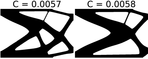
(a) Deflated Barrier (baseline, 123 min).

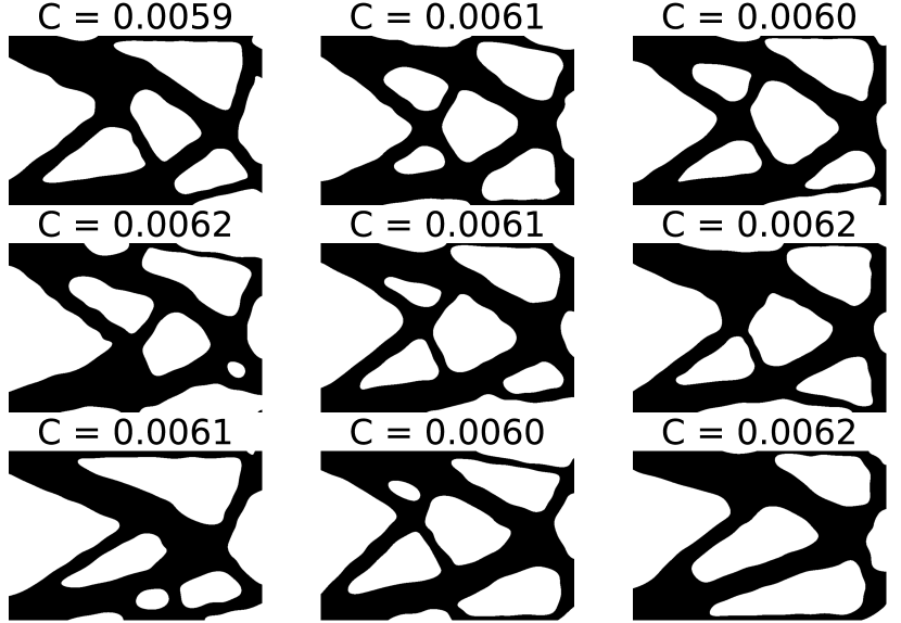
(b) GenTO (ours, 5 min).

Figure 1: Generative Topology Optimization (GenTO) produces a diverse set of near-optimal solutions on the cantilever problem defined in Figure 3(b). Compared to the baseline method, GenTO generates more shapes with greater diversity in a significantly lower time due to the inherent parallelizability. The structural compliance $C$ describes the stiffness of the shape measured as the total displacement under the load. Both methods try to minimize $C$ and achieve comparable values with similar best designs. GenTO uses a conditional neural field to parameterize the shapes forgoing adaptive mesh refinement used in the deflated barrier method.

1 Introduction

Topology optimization (TO) is a computational design technique to determine the optimal material distribution within a given design space under prescribed boundary conditions. A common objective in TO is the minimization of structural compliance, also called strain energy, which measures the displacement under load and is inverse to the stiffness of the generated design.

Due to the non-convex nature of TO problems, these methods generally provide near-optimal solutions, with no guarantees of converging to global optima (Allaire et al., 2021). Despite this, TO has been a critical tool in engineering design since the late 1980s and continues to evolve with advances in computational techniques, including the application of machine learning.

Traditional TO methods also produce a single design, which limits its utility. Engineering problems often require designs that balance performance with other considerations, such as manufacturability, cost, and aesthetics. These are associated with uncertainty, implicit knowledge, and subjectivity and are hard to optimize in a formal framework. Generating multiple diverse solutions allows for exploring these trade-offs and provides more flexibility in choosing designs that meet both technical and real-world constraints. However, conventional TO methods cannot efficiently explore and generate multiple high-quality designs in a single optimization run, making it difficult to address this need.

We propose Generative Topology Optimization (GenTO), an approach to incorporate neural networks into the TO process to generate a set of diverse designs: A neural network parametrizes the shape representations and is trained to generate near-optimal solutions. The model is optimized using a solver-in-the-loop approach (Um et al., 2020), where the neural network iteratively adjusts the design based on feedback from a physics-based solver. To enhance the diversity of solutions, we introduce an explicit diversity constraint during training, ensuring the network produces a range of solutions that still adhere to mechanical compliance objectives. GenTO not only enables the generation of multiple, diverse designs but also leverages machine learning to explore the design space more efficiently than traditional TO methods.

Empirically, we validate our method on TO for linear elasticity problems in 2D and 3D. Our results demonstrate that GenTO obtains more diverse solutions than prior work while being substantially faster, remaining near-optimal, and circumventing adaptive mesh refinement by using continuous neural fields. This addresses a current limitation in TO and opens new avenues for automated engineering design.

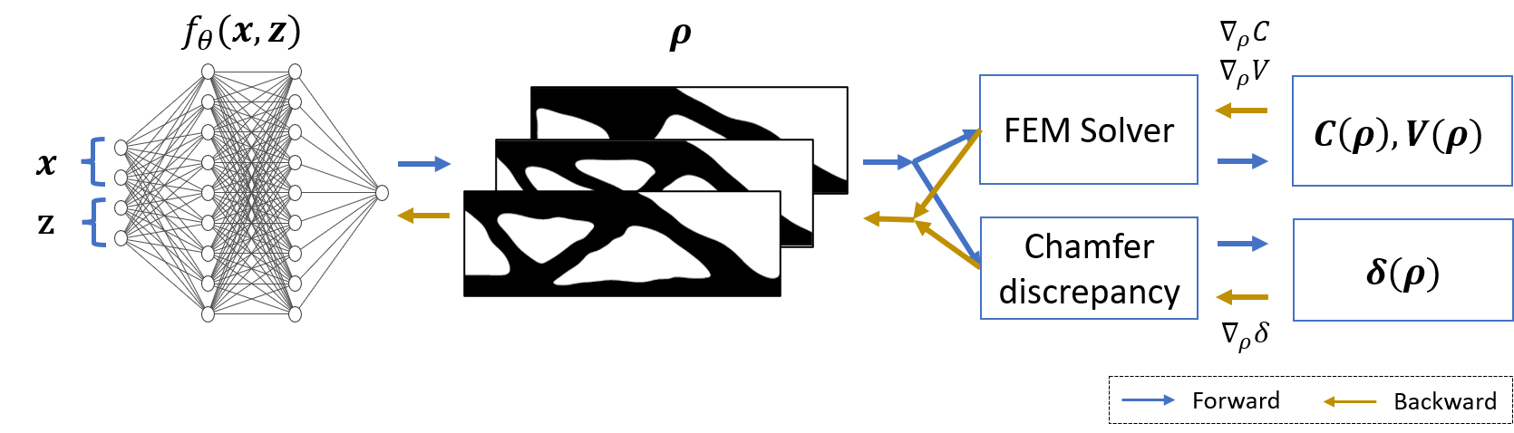
Figure 2: A single iteration of GenTO trained with 3 shapes in parallel. In each iteration, the input to the network consists of mesh locations $\mathbf{x}_{i},i\in\{1,...,N\}$ and modulation vectors $\mathbf{z}_{j},j\in\{1,...,M\}$ with $M=3$ for this example. The network outputs densities $\rho_{j}$ at mesh points $\mathbf{x}_{i}$ for each shape. The densities are passed into a FEM solver to compute compliances $C_{j}$ and volumes $V_{j}$, as well as their gradients $\nabla_{\rho}C_{j}$ and $\nabla_{\rho}V_{j}$. The diversity loss is based on the chamfer discrepancy between the surface points of the shapes. These pairwise discrepancies are used to compute the diversity loss $\delta(\rho)$ and its gradient $\nabla_{\rho}\delta$.

Our main contributions are summarized as follows:

1. We introduce GenTO, the first method for data-free, solver-in-the-loop neural network training, which generates diverse solutions adhering to structural requirements.

2. We introduce a novel diversity constraint variant for neural density fields based on the chamfer discrepancy that ensures the generation of distinct and meaningful shapes and enhances the exploration of the designs.

3. Empirically, we demonstrate the efficacy and scalability of GenTO on 2D and 3D problems, showcasing its ability to generate a variety of near-optimal designs. Our approach significantly outperforms existing methods in terms of speed and solution diversity.

2 Background

2.1 Topology optimization

Topology optimization (TO) is a computational method developed in the late 1980s to determine optimal structural geometries from mathematical formulations (Bendsøe & Kikuchi, 1988). It is widely used in engineering to design efficient structures while minimizing material usage. TO iteratively updates a material distribution within a design domain under specified loading and boundary conditions to enhance properties like stiffness and strength. Due to the non-convex nature of most TO problems, convergence to a global minimum is not guaranteed. Instead, the goal is to achieve a near-optimal solution, where the objective closely approximates the global optimum. There are four prominent method families widely recognized in TO. In this work, we focus on SIMP and refer the reader to Yago et al. (2022) for a more detailed introduction to TO.

Solid Isotropic Material with Penalization (SIMP)

is a prominent TO method we adopt for GenTO. SIMP starts by defining a mesh with mesh points $\mathbf{x}_{i}\in\mathcal{X},i\in\{1,...,N\}$ in the design region. The aim is to find a binary density function at each mesh point $\rho(\mathbf{x}_{i})\in\{0,1\}$, where $\rho(\mathbf{x}_{i})=0$ represents void and $\rho(\mathbf{x}_{i})=1$ represents solid material. To make this formulation differentiable, the material density $\rho$ is relaxed to continuous values in $[0,1]$.  A common objective of SIMP is to minimize the compliance $C$, which is a measure of the structural flexibility of a shape. Intuitively, the lower the compliance, the stiffer the shape. The SIMP objective is then formulated as a constrained optimization problem:

$$\min: \quad C(\rho)=\mathbf{u}^{T}\mathbf{K_{\rho}}\mathbf{u}$$ (1)

$$\text{s.t.}: \quad V=\sum_{i=1}^{N}\mathbf{\rho}_{i}v_{i}\leqslant V^{*}$$

$$\quad 0\leqslant\mathbf{\rho}_{i}\leqslant 1\quad\forall i\in N$$

where $\mathbf{u}$ is the displacement vector, $\mathbf{K}_{\rho}$ is the global stiffness matrix, $V$ is the shape volume, and $V^{*}$ is the target volume.  The density field is optimized iteratively. In each iteration, a finite element (FEM) solver computes the compliance and provides gradients to update the density field $\rho$. To encourage binary densities, intermediate values are penalized by raising $\rho$ to the power $p>1$. Hence, the stiffness matrix is

$$\mathbf{K}_{\rho}=\sum_{i=1}^{N}\rho_{i}^{p}\mathbf{K}_{i}$$ (2)

where $\mathbf{K}_{i}$ describes the stiffness of solid cells and depends on material properties.

Annealing

is employed to make the continuous relaxation closer to the underlying discrete problem (Kirkpatrick et al., 1983), enhancing the effectiveness of gradient-based optimization methods. Annealing gradually adjusts the sharpness of a function during the optimization. For TO, this is often done by gradually increasing the penalty $p$ or by scheduling a sharpness filter. A common choice is the Heaviside filter:

$$H(x,\beta)=0.5+\frac{\tanh(\beta(x-0.5))}{2\tanh(0.5\beta)}\$$ (3)

where $\beta$ is a parameter controlling the sharpness of the transform.

Topology optimization with neural reparametrization.

Neural reparametrization in TO provides a flexible, mesh-free way to represent shapes, offering an alternative to traditional methods. A neural network is used to learn the underlying distribution of material within a design space. Previous works have explored TO with neural networks parametrizing the density field, primarily focusing on solver-in-the-loop training (Gillhofer et al., ; Bujny et al., 2018; Chandrasekhar & Suresh, 2021; Hoyer et al., 2019), as early attempts to learn purely from data were deemed ineffective (Sosnovik & Oseledets, 2019). With GenTO we go a similar path, but learning multiple shapes with a single neural network.
NTopo (Zehnder et al., 2021) is a conceptually related approach, which employs a conditional neural field to parametrize individual solutions across multiple TO problems. Specifically, NTopo conditions the neural field on factors such as target volume or force vector position, producing a unique solution for each configuration. In contrast, GenTO extends this idea by enabling the discovery of multiple solutions for a single configuration, rather than restricting each configuration to a single solution. This ability to generate multiple valid designs broadens the potential applications of TO methodologies.

Topology optimization with multiple solutions

is important to address real-world engineering challenges, in particular when additional design considerations, such as manufacturability, and aesthetics, influence the selection of the design. By generating diverse solutions, engineers can evaluate and compare alternative designs, ultimately selecting the most suitable option in a post-processing stage. However, classical TO algorithms typically yield a single solution and do not ensure convergence to a global minimum (Papadopoulos et al., 2021).
To address this weakness, Papadopoulos et al. (2021) introduced the deflated barrier (DB) method, the first approach capable of computing multiple solutions to a given TO problem. The DB method integrates deflation techniques, barrier methods, and primal-dual active set solvers to systematically explore different local minima. By employing a search strategy akin to depth-first search, DB identifies multiple solutions without relying on initial guess variations, thereby enhancing design diversity in TO.

2.2 Shape generation with neural networks

Neural fields

offer a powerful framework for geometry processing, utilizing neural networks to model shapes implicitly. Unlike conventional explicit representations like meshes or point clouds, implicit shapes are defined as level sets of continuous functions. This approach enables high-quality and topologically flexible shape parametrizations (Chen & Zhang, 2019). The two prevalent methods for representing implicit shapes are Signed Distance Functions (SDF) (Park et al., 2019; Atzmon & Lipman, 2020) and density (or occupancy) (Mescheder et al., 2019b) fields. We opt for the density representation due to its compatibility with SIMP optimization.
A neural density field employs a neural network $f_{\theta}:\mathbb{R}^{d_{x}}\to(0,1)$ with parameters $\theta$ and the shape $\Omega$ is defined as a level-set of $f_{\theta}$. For $\tau\in\mathbb{R}$, $\Omega:=\{x\in\mathbb{R}^{d_{x}}|f_{\theta}(x)>\tau\}$, the boundary $\partial\Omega:=\{x\in\mathbb{R}^{d_{x}}|f(x)=\tau\}$, where $d_{x}\in\{2,3\}$ for 2D or 3D shapes.

Conditional neural fields.

While a neural density field represents a single shape, a conditional neural field represents a set of shapes with a single neural network (Mehta et al., 2021). To this end, a modulation code $\mathbf{z}\in\mathbb{R}^{d_{z}}$ is provided as additional input to the network. The resulting network $f_{\theta}(\mathbf{x},\mathbf{z})$ parametrizes a set of shapes, which is modulated by $\mathbf{z}$. There are different ways to incorporate the modulation vector into the network, such as input concatenation (Park et al., 2019), hypernetworks (Ha et al., 2017), or attention (Rebain et al., 2022).

Compression perspective.

A neural implicit shape can be regarded as a lossy compression of a shape into the weights of the neural network (Xie et al., 2022). As an illustrative example, consider the memory requirements of a high-fidelity shape in a voxel representation compared to a neural density representation. While the neural implicit shape might not perfectly approximate the voxel representation, it requires fewer bits of storage. For conditional neural fields, the compression factor is usually higher, as the network does not have to store the mutual information between the shapes for each shape individually.

Diversity constraint.

To discover multiple solutions during optimization, we add a diversity constraint to the problem formulation (1). The diversity constraint introduced by GINNs (Berzins et al., 2024) defines a diversity measure $\delta$ on the set of shapes $\{\Omega_{i}\}$ as follows:

$$\delta(\{\Omega_{i}\})=\left(\sum_{j}\left(\min_{k\neq j}d(\Omega_{j},\Omega_{k})\right)^{1/2}\right)^{2}\ .$$ (4)

This measure builds upon a chosen dissimilarity function $d(\Omega_{i},\Omega_{j})$. Essentially, $\delta$ encourages diversity by maximizing the distance between each shape and its nearest neighbor. GINNs utilize a dissimilarity function defined on the boundaries: $d(\Omega_{1},\Omega_{2})=\sqrt{\int_{\partial\Omega_{i}}f_{j}(x)^{2}d{x}+\int_{\partial\Omega_{j}}f_{i}(x)^{2}d{x}}$. The authors demonstrated that for SDFs $f_{1}$ and $f_{2}$ of the shapes $\Omega_{1}$ and $\Omega_{2}$, this corresponds to the chamfer discrepancy. However, this result relies on the SDF assumption that $f_{i}(x)$ measures the distance of the point $x$ to the boundary $\partial\Omega_{i}$. It does not hold for more general implicit representations, such as the density fields we use. Therefore, we derive an alternative dissimilarity function tailored for density fields in Section 3.2.

3 Method

3.1 Generative Topology Optimization

Definitions.

Let $\mathcal{X}\subset\mathbb{R}^{d_{x}}$ be the domain of interest in which there is a shape $\Omega\subset\mathcal{X}$. Let $\mathcal{Z}\subset\mathbb{R}^{d_{z}}$ be a discrete or continuous modulation space, where each $\mathbf{z}\in\mathcal{Z}$ parametrizes a shape $\Omega_{\mathbf{z}}$. The possibly infinite set of all shapes is denoted by $\Omega_{\mathcal{Z}}=\{\Omega_{\mathbf{z}}|\mathbf{z}\in\mathcal{Z}\}$. The modulation vectors $\{\mathbf{z}_{i}\}$ are either elements in a fixed, finite set $\mathcal{Z}$ or sampled according to a continuous probability distribution $p(\mathcal{Z})$ on an interval $[a,b]^{n}\subset\mathbb{R}^{n}$. For brevity, we will use $\mathbf{z}\sim p(\mathcal{Z})$ for both of these cases.
For density representations a shape $\Omega_{\mathbf{z}}$ is defined as the set of points with a density greater than the level $\tau\in[0,1]$, formally $\Omega_{\mathbf{z}}=\{\mathbf{x}\in\mathcal{X}\mid\rho_{\mathbf{z}}(\mathbf{x})>\tau\}$. While some priors work on occupancy networks (Mescheder et al., 2019a) treat $\tau$ as a tunable hyperparameter, we follow Jia et al. (2024) and fix the level at $\tau=0.5$. We model the density $\rho_{\mathbf{z}}(\mathbf{x})=f_{\theta}(\mathbf{x},\mathbf{z})$, corresponding to the modulation vector $\mathbf{z}$ at a point $\mathbf{x}$ using a neural network $f_{\theta}$, with $\theta$ being the learnable parameters.

Algorithm 1 GenTO

 Input: parameterized density $f_{\theta}$, vector of mesh points $\mathbf{x_{i}}\in\mathbb{R}^{d_{x}}$, $\beta$ and annealing factor $\Delta_{\beta}$, number of shapes per iteration $k$, learning rate scheduler $\gamma(t)$, iterations $T$

 for $t=1$ to $T$ do

  $\mathbf{z_{j}}\sim p(\mathcal{Z})$ {sample modulation vectors}

  $\tilde{\rho}_{z_{j}}\leftarrow f_{\theta}(\mathbf{x_{i}},\mathbf{z_{j}})$ {net forward all shapes $j$}

  $\rho_{j}\leftarrow H(\tilde{\rho}_{z_{j}},\beta)$ {Heaviside contrast filter}

  $C,V,\frac{\partial C}{\partial\rho},\frac{\partial V}{\partial\rho}\leftarrow\text{FEM}(\rho_{j})$ {solver step}

  $\frac{\partial\rho}{\partial\theta}\leftarrow\text{backward}(f_{\theta},\rho_{j})$ {autodiff backward}

  $\nabla_{\theta}C\leftarrow\frac{\partial C}{\partial\rho}\frac{\partial\rho}{\partial\theta}$ {compliance gradient}

  $\nabla_{\theta}V\leftarrow\lambda_{V}\frac{\partial C}{\partial\rho}\frac{\partial\rho}{\partial\theta}$ {volume gradient}

  $L_{\text{G}}\leftarrow\lambda_{\text{interface}}L_{\text{interface}}+...$  {GINN constraints}

  $\Delta\theta\leftarrow\text{ALM}\left(\nabla_{\theta}C,\nabla_{\theta}V,\nabla_{\theta}L_{\text{G}}\right)$ {ALM}

  $\theta\leftarrow\theta-\gamma(t)\Delta\theta$ {parameter update}

  $\beta\leftarrow\beta\Delta_{\beta}$ {annealing}

 end for

GenTO

aims to solve a constrained optimization problem with the objective of minimizing the expected compliance of multiple shapes subject to a volume constraint on each. At the core of our method is the diversity constraint $\delta(\Omega_{\mathcal{Z}})$, defined over multiple shapes to make them less similar. This leads to the following constrained optimization problem:

$$\min: \quad\mathbb{E}_{\mathbf{z}\sim p(\mathcal{Z})}\left[C(\rho_{\mathbf{z}})\right]$$ (5)

$$\text{s.t.}: \quad V_{\mathbf{z}}=\int_{\mathcal{X}}\mathbf{\rho}_{\mathbf{z}}(\mathbf{x})d\mathbf{x}\leqslant V^{*}$$

$$\quad 0\leqslant\mathbf{\rho}_{\mathbf{z}}(\mathbf{x})\leqslant 1$$

$$\quad\delta^{*}\leqslant\delta(\Omega_{\mathcal{Z}})$$

where $V^{*}$ and $\delta^{*}$ are target volumes and diversities, respectively. GenTO updates the density fields of multiple shapes iteratively. In each iteration, the density distribution of each shape is computed and the resulting densities are passed to a finite element method (FEM) solver. The FEM solver calculates the compliance loss $C$ and gradients $\nabla C$ using the adjoint equation instead of differentiating through the solver. To accelerate the computation, parallelization of the FEM solver is employed across multiple CPU cores, with a separate process dedicated to each shape.
The diversity loss (see Section 3.2) is computed on the GPU, along with any optional geometric losses similar to GINNs (see Section 3.3). Gradients for these losses are obtained via automatic differentiation, based on which GenTO updates the network parameters $\theta$.
We use the adaptive augmented Lagrangian method (ALM) (Basir & Senocak, 2023) to automatically balance multiple loss terms. Additionally, we gradually increase the sharpness parameter $\beta$ of the Heaviside filter (Equation 3) which acts as annealing. This outline of the GenTO method is summarized in Algorithm 1.

3.2 Diversity

The diversity loss, defined in Equation 4, requires the definition of a dissimilarity measure between a pair of shapes. Generally, the dissimilarity between two shapes can be based on either the volume of a shape $\Omega$ or its boundary $\partial\Omega$. GINNs (Berzins et al., 2024) use boundary dissimilarity, which is easily optimized for SDFs since the value at a point is the distance to the zero level set. However, this dissimilarity measure is not applicable to our density field shape representation. Hence we propose a boundary dissimilarity based on the chamfer discrepancy in the We also developed a volume-based dissimilarity (detailed in Appendix C.1), however we focus on boundary diversity due to its promising results in early experiments.

Diversity on the boundary via differentiable chamfer discrepancy.

To define the dissimilarity on the boundaries of a pair of shapes $(\partial\Omega_{1},\partial\Omega_{2})$, we use the one-sided chamfer discrepancy (CD):

$$\text{CD}(\partial\Omega_{1},\partial\Omega_{2})=\frac{1}{\left|\partial\Omega_{1}\right|}\sum_{x\in\partial\Omega_{1}}\min_{\tilde{x}\in\partial\Omega_{2}}||x-\tilde{x}||_{2}$$ (6)

where $x$ and $\tilde{x}$ are sampled points on the boundaries. To use the CD as a loss, it must be differentiable w.r.t. the network parameters $\theta$. However, the chamfer discrepancy $\text{CD}(\partial\Omega_{1},\partial\Omega_{2})$ depends only on the boundary points $x_{i}\in\partial\Omega$ which only depend on $f_{\theta}(x_{i})$ implicitly. Akin to prior work (Chen et al., 2010; Berzins et al., 2023; Mehta et al., 2022), we apply the chain rule and use the level-set equation to derive

$$\frac{\partial\text{CD}}{\partial\theta}=\frac{\partial\text{CD}}{\partial x}\frac{\partial x}{\partial y}\frac{\partial y}{\partial\theta}=\frac{\partial\text{CD}}{\partial x}\frac{\nabla_{x}f_{\theta}}{|\nabla_{x}f_{\theta}|^{2}}\frac{\partial y}{\partial\theta}$$ (7)

where $y=\rho$ is the density field in our case. We detail this derivation in Appendix C.3.

Finding surface points on density fields.

Finding surface points for densities is substantially harder than for SDFs. For an SDF $f$, surface points can be obtained by flowing randomly initialized points along the gradient $\nabla f$ to the boundary at $f=0$. However, density fields $g$ do not satisfy the eikonal equation $|\nabla g|\neq 1$, causing gradient flows to easily get stuck in local minima. To overcome this challenge, we employ a robust algorithm that relies on dense sampling and binary search, as detailed in Algorithm 2.

3.3 Formalizing geometric constraints

The compliance and volume losses are computed by the FEM solver on a discrete grid. In addition, we use geometric constraints similar to GINNs. This leverages the continuous field representation and allows learning finer details where necessary, e.g. at the interfaces. In principle, these constraints could also be imposed via the TO framework, by defining solid regions ($\rho=1$ values) to specific mesh cells. However, this comes at the cost of requiring increased mesh resolution, which raises the computational cost for the CPU-based FEM solver. Instead, we adapt the geometric constraints of GINNs to operate with a general level set $\tau$ and reflect the change from an SDF to a density representation. The applied constraints and further details are in Table 2 and Appendix B. Crucially, these are computed in parallel on the GPU, accelerating the optimization process.

4 Experiments

For all our GenTO experiments, we employ the WIRE architecture (Saragadam et al., 2023), which uses wavelets as activation functions. This imposes an inductive bias towards high-frequencies, while being more localized than, e.g., a sine activation (Sitzmann et al., 2020). We use a 2-dimensional modulation space $Z\subset\mathbb{R}^{2}$, where most runs use $Z=[0,1]^{2}$.

We perform 3 different runs for GenTO. GenTO (single) optimizes a single shape and serves as a baseline for compliance. The diversity constraint is not included, as it is trivially 0. GenTO (equidistant) optimizes $M=9$ shapes in a single iteration in all experiments. The $M$ modulation vectors $\mathbf{z}_{j}$ are taken from $\mathcal{Z}\subset\mathbb{R}^{2}$ in an equidistant $3\times 3$ grid at the beginning of training. GenTO (uniform) optimizes a set of shapes, with the number of shapes $M$ being either 9 or 25, depending on the experiment. In every iteration, $M$ modulation vectors are sampled uniformly from $\mathcal{Z}$. By uniformly sampling from $\mathcal{Z}$ the network learns a set of shapes.

For training GenTO, the FEM solver mesh resolution (see 1) is kept constant throughout training. Further experimental details and hyperparameters can be found in Appendix A.

4.1 Problem definitions

We apply our method to common linear elasticity problems in two and three dimensions, described below and depicted in Figure 3.

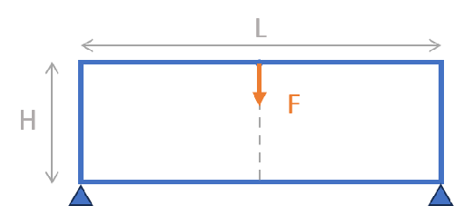
(a)

(b)

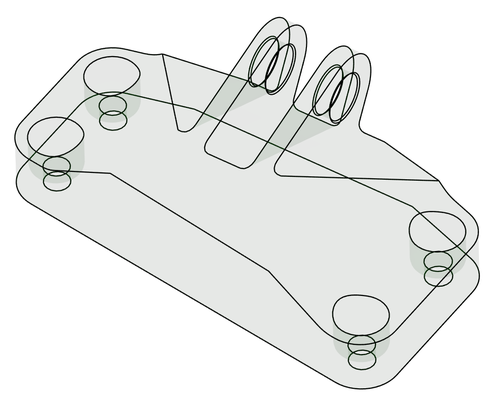
(c)

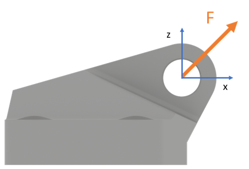
(d)

Figure 3: Illustration of the problem definitions, design regions, and load cases. (a) MBB Beam: The boundary is fixed at the attachment points at the bottom left and right corners. The dotted line indicates the symmetry axis at $\frac{L}{2}$ where the force $F$ is applied. (b) Cantilever: Forces $F_{1}$, $F_{2}$ are applied at distance $h$ from the upper and lower boundaries. The left boundary is fixed to the wall. (c) Jet engine bracket design region: Solution shapes must be contained within the design region and attach to the six cylindrical interfaces. (d) Jet engine bracket load case: A diagonal force is applied at the two central interfaces. The bracket is fixed at the four side interfaces.

Messerschmitt-Bölkow-Blohm beam (2D).

The MBB beam is a common benchmark problem in TO and is depicted in Figure 3(a). The problem describes a beam fixed on the lower right and left edges with a vertical force $F$ applied at the center. As the problem is symmetric around $x=L/2$, we follow Papadopoulos et al. (2021) and only optimize the right half.
The concrete dimensions of the beam are $H=1,L=6$ and the force points downwards with $F=1$.

Cantilever beam (2D).

The cantilever beam is illustrated in Figure 3(b). The problem describes a beam fixed on the left-hand side and two forces $F_{1}$, $F_{2}$ are applied on the right-hand side.
The dimensions are $H=1,L=1.5,h=0.1$ and the forces $F_{1}=F_{2}=0.5$.

Jet engine bracket (3D).

We apply GenTO to a challenging 3D task, namely the optimization of a jet engine bracket as defined by Kiis et al. (2013). The design region for this problem is given via a surface mesh (see Figure 3(c)). The load case is depicted in Figure 3(d) in which a diagonal force pulls in positive x and positive z direction.

4.2 Baselines

TO for a single solution.

The main baseline for TO for a single solution is a standard implementation of SIMP. We rely on FeniTop (Jia et al., 2024), a well-documented implementation of SIMP. Single-shape reference solutions for all problems are shown in Appendix A.3.
FeniTop applies a smoothing filter to the densities before passing them to the FEM solver. This avoids checkerboard patterns caused by the numerical error of FEM (Sigmund & Petersson, 1998). As GenTO, FeniTop also uses contrast filters (more details on filters in Appendix A.1).

TO for multiple solutions.

The deflated barrier method (DB) (Papadopoulos et al., 2021) is the state-of-the-art method for finding multiple solutions to TO problems. In contrast to GenTO, DB is a sequential algorithm and cannot perform multiple solver steps in parallel. For linear elasticity, the deflated barrier method only provides an implementation for the cantilever and MBB beam. A comparison between GenTO and DB for the jet engine bracket is omitted, given DB’s complex mathematical framework, slower performance (see Section 5), and hyperparameter sensitivity. Notice that the available implementation of DB refines the mesh during training, which increases the runtime per solver step during optimization.

4.3 Metrics

Unlike DB and TO, which generate single solutions, GenTO has the capability to produce a potentially infinite set of shapes. $\Omega_{\mathcal{Z}}=\{\Omega_{\mathbf{z}}\mid\mathbf{z}\in\mathcal{Z}\}$. During training, shapes are sampled according to a probability distribution $p(\mathcal{Z})$. Hence, our metrics are based on the expected value over $p(\mathcal{Z})$.

Quality.

For structural efficiency, we use the expected compliance $\mathbb{E}[C]\coloneqq\mathbb{E}_{z\sim p(\mathcal{Z})}[C(\Omega_{\mathbf{z}})]$, as well as minimum compliance $\min(C)\coloneqq\min_{\mathbf{z}\in\mathcal{Z}}C(\Omega_{\mathbf{z}})$ and maximum compliance $\max(C)\coloneqq\max_{\mathbf{z}\in\mathcal{Z}}C(\Omega_{\mathbf{z}})$. To verify that the volume constraint is satisfied, we use the expected volume $\mathbb{E}[V]\coloneqq\mathbb{E}_{z\sim p(\mathcal{Z})}[V(\Omega_{\mathbf{z}})]$ over obtained shapes. We use the FenicsX numerical solver (Baratta et al., 2023) to compute compliance and volume values. For each problem, we use a high-resolution mesh to compute the final compliance metrics for all methods. This minimizes the discretization error in the compliance computation and prevents numerical artifacts due to the mesh dependency of the solver.

Diversity.

A diversity measure shall capture several natural properties, accounting, e.g., for the number of elements and the dissimilarity between elements of a set. Leinster (2021) states 6 natural properties and rigorously proves that only the Hill numbers $D_{q}(S),q\in\mathbb{R}$ over a set $S$ fulfill these properties all at once. If $q=2$, the Hill number is interpretable, as it corresponds to the expected dissimilarity if 2 elements of a set are sampled with replacement. Hence, we choose $D_{2}(\Omega_{\mathcal{Z}})$. to measure the diversity of shapes $\Omega_{\mathcal{Z}}$, we follow Leinster (2021) and report the expected Wasserstein-1 distance between the shapes in the set:

$$\mathbb{E}[W_{1}]\coloneqq\mathbb{E}_{\mathbf{z}_{i},\mathbf{z}_{j}\sim p(\mathcal{Z})}\left[W_{1}(\Omega_{\mathbf{z}_{i}},\Omega_{\mathbf{z}_{j}})\right]$$ (8)

where $W_{1}(\Omega_{\mathbf{z}_{i}},\Omega_{\mathbf{z}_{j}})$ is the sliced-1 Wasserstein distance (Flamary et al., 2021), a computationally cheaper variant of the Wasserstein distance. Importantly, $z_{i},z_{j}$ are sampled with replacement as rigorously derived by Leinster (2021).

Computational cost.

To compare the computational cost of different methods, we report the number of solver steps, since for large meshes (e.g., more than 10K elements) this becomes the main computational bottleneck. In addition, we use the number of iterations of the network (i.e. optimizer steps), as these take into account the parallelization of GenTO. We also report wall clock time, as it gives a sense of the practicality of a method.

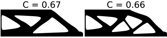
(a) Deflated Barrier (baseline, 55 min).

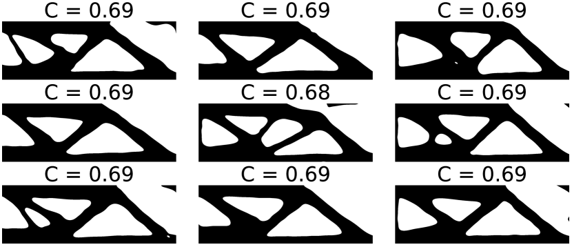
(b) GenTO (ours, 4 min).

Figure 4: Comparison of results for the MBB beam. Similar to the cantilever problem in Figure 1, GenTO produces more diverse results than the DB baseline in much less time with similar compliance values.

5 Results

5.1 Main results

The quantitative results of our experiments are summarized in Table 1. Qualitatively, we show different results in Figures 1, 4, and 5. To validate that GenTO can produce good single results on par with the baseline, comparisons of FeniTop and GenTO (single) are shown in the Appendix in Figures 6, 7 and 8.

GenTO is more diverse.

Across all our experiments, we observe that GenTO finds more diverse solutions than DB. Note, that the solutions also vary in their topology, i.e. have a different number of holes.

Table 1: Experimental results on the three linear elasticity problems. $\mathbf{N}$ is the number of solutions, $\mathbb{E}(\mathbf{C})$, $\min(\mathbf{C})$, and $\max(\mathbf{C})$ are the average, minimum, and maximum compliance values of the solutions (lower is better). $\mathbb{E}(V)$ is the mean volume of the solutions in percent of the volume in the design region, $\mathbb{E}(W_{1})$ is the expected Wasserstein-1 distance between solutions quantifying the diversity (higher is better). Time is the wall clock time in minutes, Its. is the number of iterations until convergence, Steps is the number of FEM solver calls, and FEM resolution is mesh resolution used by the FEM solver. Note that the FEM resolution of DB changes over time due to the adaptive mesh refinement (indicated by initial grid $\rightarrow$ final refined mesh size).

Problem	Method	$\mathbf{N}$	$\mathbb{E}(\mathbf{C})$	$\min(\mathbf{C})$	$\max(\mathbf{C})$	$\mathbb{E}(V)$	$\mathbb{E}(W_{1})$	Time	Its.	Steps	FEM resolution
MBB						53.5
	DB	2	0.67	0.66	0.67	53.49	0.0136	55.5		3190	50x150 $\rightarrow$ 27174
	FeniTop	1	0.68			53.49		2	400	400	180x60
	GenTO (single)	1	0.68			54.09		1.5	400	400	180x60
	GenTO (equidistant)	9	0.69	0.68	0.69	53.54	0.0214	4	400	3600	180x60
	GenTO (uniform)	$\mathcal{U}([0,1]^{2})$	0.70	0.69	0.72	53.28	0.0157	13	650	16250
Cantilever				$\times 10^{-2}$		50.00
	DB	2	0.58	0.57	0.58	49.98	0.0101	123		4922	25x37 $\rightarrow$ 52024
	FeniTop	1	0.59			49.91		4	400	400	150x100
	GenTO (single)	1	0.58			49.94		2.5	400	400	150x100
	GenTO (equidistant)	9	0.61	0.59	0.62	50.42	0.0157	5	400	3600	150x100
	GenTO (uniform)	$\mathcal{U}([0,1]^{2})$	0.67	0.65	0.73	49.60	0.0065	28.5	1000	25000	150x100
Bracket				$\times 10^{-3}$		7.00
	FeniTop	1	0.99			7.16		187	300	400	104x172x60
	GenTO (single)	1	0.90			7.42		19.5	400	400	26x43x15
	GenTO (equidistant)	9	0.97	0.87	1.04	7.07	0.0065	60	1000	9000	26x43x15
	GenTO (uniform)	$\mathcal{U}([0,0.25]^{2})$	1.63	1.35	1.85	7.04	0.0015	92	1400	12600	26x43x15

GenTO is faster.

Compared to DB, GenTO with equidistant sampling is more than an order of magnitude faster in terms of wall clock time. The main reason is the parallelism of GenTO, while DB is an inherently sequential algorithm. Note, that DB performs mesh refinement in certain stages, which increases the time per solver step. GenTO with equidistance sampling is approximately on par with DB in terms of total solver steps.

Equidistant beats uniform sampling.

Across all experiments, equidistant sampling performs better than uniform sampling for all considered metrics. We attribute this to the fact that for equidistant sampling, the network can learn to cover important modes which are sufficiently far away from each other, without needing to find good intermediate shapes. In contrast, when modulation is sampled uniformly, the network must learn a continuous encoding of solutions. This typically requires more iterations and solver steps than other methods due to the additional complexity.

Single solutions beat multiple solutions.

In terms of compliance, speed, and solver steps, single solutions beat multiple solutions in all experiments. This is expected, as the optimization for multiple solutions additionally accounts for the diversity constraint. Notably, the single solution for GenTO is on par with FeniTop, but worse than DB. This is partially expected, as DB refines the mesh during optimization.

Figure 5: Three different jet engine bracket designs generated by GenTO. Left: top view. Right: isometric view. Notably, all three generated designs show the same low compliance as the single solution by the FeniTop baseline. These explored solutions can be further refined and post-processed by a classical pipeline.

5.2 Ablations

We perform ablations to highlight important design decisions of GenTO. The main findings are described in the following and additionally visualized in Appendix A.5.

Sensitivity to penalty $p$.

For SIMP, the density is penalized with an exponent $p$ (see Equation 2). Our experiments show that GenTO is sensitive to the choice of $p$, as it sharpens the loss landscape. This becomes more apparent when looking at the derivative of the stiffness of a mesh element $\frac{\partial\mathbf{K}_{i}(\rho_{i})}{\partial\rho_{i}}=p\rho_{i}^{p-1}\mathbf{K}_{i}$. E.g., for $p=3$ the gradient is quadratically scaled by the current density value. This implies that the higher $p$, the harder it is to escape local minima. We do not observe a large performance impact in the 2D experiments. However, in 3D, we observe that $p=3$ instead of $p=1.5$ leads to convergence to an undesired local minimum, illustrated in Figure 15(a).

Annealing is necessary for good convergence.

We find that GenTO requires annealing to achieve good convergence. Figure 15(b) demonstrates a failed run without $\beta$ scheduling the Heaviside function (Equation 3).

Different frequency bias for $\mathbf{x}$ and $\mathbf{z}$.

The importance of frequency bias has been highlighted by several works (Sitzmann et al., 2020; Saragadam et al., 2023). Importantly, depending on the problem, there might be a different frequency bias necessary for the coordinates $\mathbf{x}$ and the modulation vectors $\mathbf{z}$. For the WIRE architecture we use in our experiments, the frequency bias of the modulation is implicitly controlled by the (hyper-) volume of $\mathcal{Z}$. This controls the diversity at initialization and convergence as suggested by Teney et al. (2024). Figure 16 shows solutions to the MBB beam for $\mathcal{Z}=[0,0.1]^{2}$. Compared to the better tuned $\mathcal{Z}=[0,1]^{2}$ in Figure 16, the diversity almost halves from $21.4\times 10^{-3}$ to $11.8\times 10^{-3}$.

6 Conclusion

This paper presents Generative Topology Optimization (GenTO), a novel approach that addresses a limitation in traditional TO methods. By leveraging neural networks to parameterize shapes and enforcing solution diversity as an explicit constraint, GenTO enables the exploration of multiple near-optimal designs. This is crucial for industrial applications, where manufacturing or aesthetic constraints often necessitate the selection of alternative geometries. Our empirical results demonstrate that GenTO is both effective and scalable, generating more diverse solutions than prior methods while adhering to mechanical requirements. Our main contributions include the introduction of GenTO as the first data-free, solver-in-the-loop neural network training method and the empirical demonstration of its effectiveness across various problems. This work opens new avenues for generative design approaches that do not rely on large datasets, addressing current limitations in engineering and design.

Limitations and future work.

While GenTO shows notable progress, several areas warrant further investigation to fully realize its potential. Qualitatively, we observe, e.g. in Figure 4(b), that shapes produced by GenTO can contain floaters (small disconnected components) and have surface undulations. This warrants further investigation and can be preliminarily corrected by post-processing steps (Subedi et al., 2020).
More research is needed to explore different dissimilarity metrics for the diversity loss, as this could further enhance the variety of generated designs. Improving sample efficiency is also crucial for practical applications, as the current method may require significant computational resources. Promising directions include using second-order optimizers and using the mutual information of concurrent solver outputs at early training stages. Lastly, future work could train GenTO on coarse designs and subsequently refine them with classical TO methods, combining the strengths of both approaches to achieve even better results.

Appendix A Implementation and experimental details

A.1 Smoothing and contrast filtering

Filtering is a general concept in topology optimization, which aims to reduce artifacts and improve convergence. Helmholtz PDE filtering is a smoothing filter similar to Gaussian blurring, but easier to integrate with existing finite element solvers. By solving a Helmholtz PDE the material density $\rho$ is smoothened to prevents checkerboard patterns, which is typical for TO (Lazarov & Sigmund, 2011). Heaviside filtering is a type of contrast filter, which enhances the distinction between solid and void regions. The Heaviside filter function equals the sigmoid function up to scaling of the input. We therefore denote $\rho_{h}$ as the Heaviside-filtered $\rho$ as defined in Equation 3 Whereas $\beta$ is a parameter controlling the sharpness of the transform, similar to the inverse temperature of a classical softmax (higher beta means a closer approximation to a true Heaviside step function). Note that in contrast to the Helmholtz PDE filter, the heaviside filter is not volume preserving. Therefore the volume constraint has to be applied to the modified output.

A.2 Model hyperparameters

We report additional information on the experiments and their implementation. We run all experiments on a single GPU (NVIDIA Titan V12), but potentially across multiple CPU cores (up to 32). For single-shape training, the maximum GPU memory requirements are less than 2GB for all experiments.

For the model to effectively learn high-frequency features, it is important to use a neural network represenation with a high frequency bias (Sitzmann et al., 2020; Teney et al., 2024). Hence, all models were trained using the real, 1D variant of the WIRE architecture (Saragadam et al., 2023). WIRE allows to adjust the frequency bias by setting the hyperparameters $\omega_{0}^{1}$ and $s_{0}$. For this architecture, each layer consists of 2 Multi-layer perceptron (MLPs), one has a periodic activation function $cos(\omega_{0}x)$, the other with a gaussian $e^{(s_{0}x)^{2}}$. The post-activations are then multiplied element-wise.

	MBB Beam	MBB Beam	Cantilever	Cantilever	JEB	JEB
Sampling	equidistant	uniform	equidistant	uniform	equidistant	uniform
Hidden layers	32x3	32x3	32x3	32x3	64x3	64x3
$\omega_{0}^{1}$ for WIRE	18	18	18	18	18	18
$s_{0}$ for WIRE	20	20	10	10	6	6
Learning rate	$10^{-4}$	0.0001	0.0001	0.0001	0.001	0.001
$\mathcal{Z}$	$[0,1]^{2}$	$[0,1]^{2}$	$[0,1]^{2}$	$[0,1]^{2}$	$[0,0.25]^{2}$	$[0,0.25]^{2}$
SIMP penalty $p$	3	3	3	3	1.5	1.5
$\beta$ annealing	$[0,400]$	$[0,400]$	$[0,400]$	$[0,400]$	$[0,400]$	$[0,400]$
$\hat{\delta}(\Omega_{\mathcal{Z}})$	0.2	0.06	0.3	0.25	0.15	0.15
# iterations	400	650	400	1000	1000	1000
# shapes per batch	9	25	9	25	9	9

A.3 Reference Solutions

We provide reference solutions to the problem settings generated by standard topology optimization (TO). We use the implementation of the SIMP method provided by the FeniTop library Jia et al. (2024) as classical TO baseline.
We also generate single solutions using GenTO without a diversity constraint or modulation variable as input. These single shape training runs showcase the baseline capability of GenTO.
The reference solutions for MBB beam problem are shown in Figure 6, for the cantilever beam problem in Figure 7 and for the jeb engine bracket problem in Figure 8.

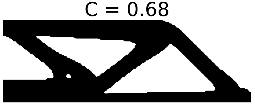
(a) Single solution generated with FeniTop

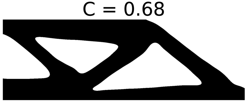
(b) Single solution generated with GenTO

Figure 6: Reference solutions for the MBB beam problem

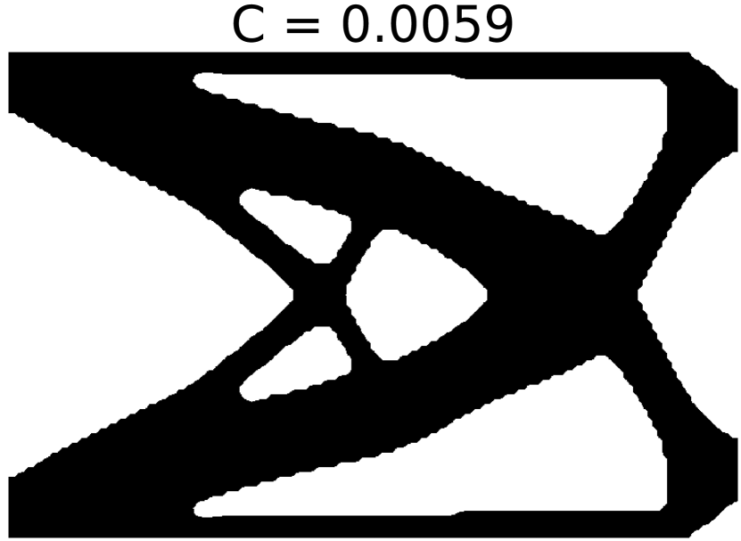
(a) Single solution generated with FeniTop

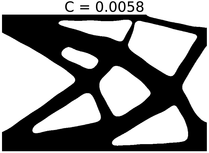
(b) Single solution generated with GenTO

Figure 7: Reference solutions for the Cantilever problem

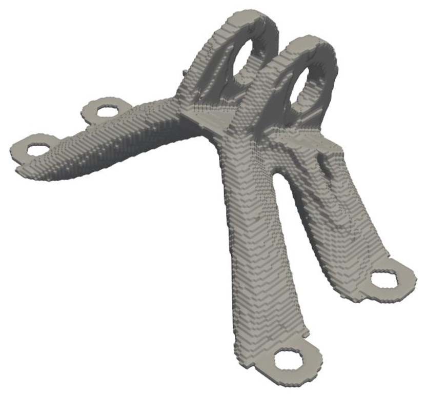
(a) Single solution generated with FeniTop

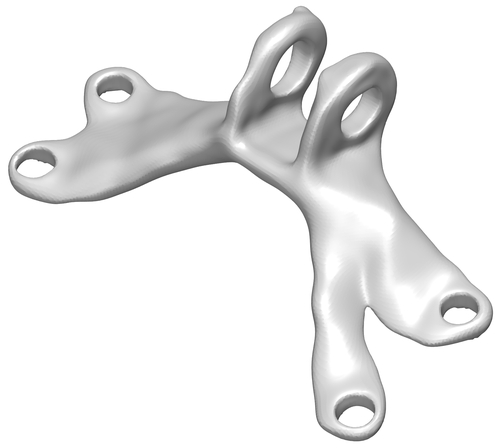
(b) Single solution generated with GenTO

Figure 8: Reference solutions for the jet engine bracket (JEB) problem

A.4 Additional Results

We show additional qualitative results for our experiments.

MBB beam

Figure 9 shows the MBB beam, which was uniformly sampled during training, evaluated at equidistant points $\mathbf{z}\in\mathcal{Z}$.

Figure 9: MBB beam uniformly sampled during training from $\mathcal{Z}=[0,1]^{2}$. The depicted shapes for this figure are sampled equidistantly from $\mathcal{Z}$.

Cantilever

Figure 10 shows the Cantilever, which was uniformly sampled during training, evaluated at equidistant points $\mathbf{z}\in\mathcal{Z}$.

Figure 10: Cantilever uniformly sampled during training from $\mathcal{Z}=[0,1]^{2}$. The depicted shapes for this figure are sampled equidistantly from $\mathcal{Z}$.

Jet engine bracket

Figure 11 and Figure 12 show the results of the Jet engine bracket (JEB), which was equidistantly taken from $\mathbf{z}\in\mathcal{Z}=[0,0.25]$ at the start of training. Figure 13 and Figure 14 show the results of a Jet engine bracket (JEB), which was uniformly sampled at each iteration $\mathbf{z}\in\mathcal{Z}=[0,0.25]$.

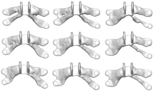
Figure 11: JEB (equidistant) top view: The depicted shapes for this figure are sampled equidistantly from $\mathcal{Z}=[0,0.25]^{2}$.

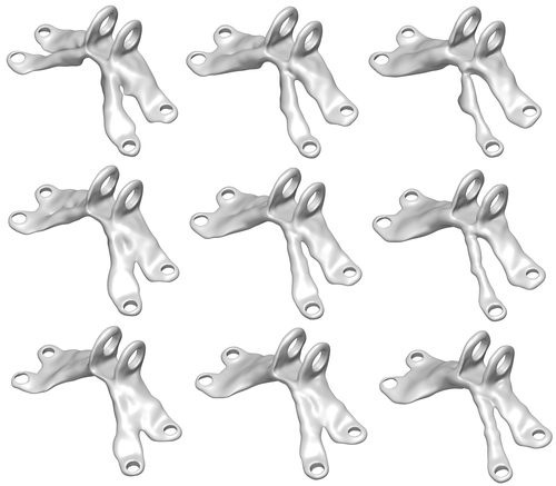
Figure 12: JEB (equidistant) diagonal view: The depicted shapes for this figure are sampled equidistantly from $\mathcal{Z}=[0,0.25]^{2}$.

Figure 13: JEB (uniform) top view: During training, modulation vectors $\mathbf{z}$ for this figure are sampled uniformly from $\mathcal{Z}=[0,0.25]^{2}$.

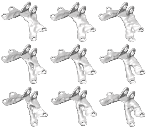
Figure 14: JEB (uniform) diagonal view: During training, modulation vectors $\mathbf{z}$ for this figure are sampled uniformly from $\mathcal{Z}=[0,0.25]^{2}$.

A.5 Ablations

We show additional figures for the ablations in Section 5.2.

Penalty $p=3$

Tuning the penalty is important for GenTO to work. We demonstrate this in Figure 15(a). The shape converges to a unfavorable local minimum as the loss landscape is too sharp.

No annealing.

For Figure 15(b), the annealing was turned off. The optimization fails to converge to a useful compliance value and does not fulfill the desired interface constraints.

(a)

(b)

Figure 15: Ablations for penalty and $\beta$ annealing. (a) Jet engine bracket trained with penalty $p=3$. (b) Jet engine bracket trained without annealing.

Modulation space $\mathcal{Z}$

Figure 16 depicts the results of an MBB beam where the modulation space $\mathcal{Z}$ has a too low volume.

The resulting shapes are not as diverse despite applying the diversity constraint during training.

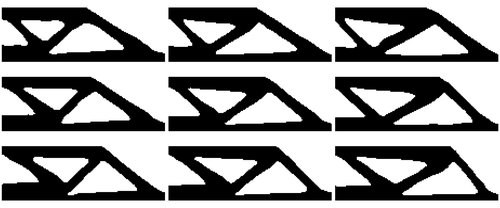
Figure 16: MBB beam results for an equidistantly sampled modulation space of $\mathcal{Z}=[0,0.1]^{2}$. The diversity metric is $0.0214$.

Appendix B Geometric constraints

We formulate geometric constraints analogously to GINNs in Table 2 for density representations. There are two important differences when changing the shape representation from a signed distance function (SDF) to a density function.
First, the level set $\partial\Omega_{\tau}$ changes from $\partial\Omega_{\tau}=\left\{x\in\mathbb{R}^{d_{x}}|f_{\theta}=0\right\}$ to $\partial\Omega_{\tau}=\left\{x\in\mathbb{R}^{d_{x}}|f_{\theta}=0.5\right\}$. Second, for a SDF the shape $\Omega_{tau}$ is defined as the sub-level set $\Omega_{\tau}=\left\{x\in\mathbb{R}^{d_{x}}|f_{\theta}\leqslant 0\right\}$ , whereas for a density it is the super-level set $\Omega_{\tau}=\left\{x\in\mathbb{R}^{d_{x}}|f_{\theta}\geq 0\right\}$.

Table 2: Geometric constraints are derived from GINNs. The shape $\Omega$ and its boundary $\partial\Omega$ are implicitly defined by the level set $\tau$ of the function $f$. The shape must reside within the design region $\mathcal{E}\subseteq\mathcal{X}$ and adhere to the interface $\mathcal{I}\subset\mathcal{E}$ with a specified normal $\bar{n}(x)$.

	Set constraint $c_{i}(\Omega)$	Function constraint	Constraint violation $c_{i}(f)$
Design region	$\Omega\subset\mathcal{E}$	$f(x)<\tau\ \forall x\notin\mathcal{E}$	$\int_{\mathcal{X}\setminus\mathcal{E}}\left[\operatorname{max}(0,f(x)-\tau)\right]^{2}dx$
Interface	$\partial\Omega\supset\mathcal{I}$	$f(x)=\tau\ \forall x\in\mathcal{I}$	$\int_{\mathcal{I}}\left[f(x)-\tau\right]^{2}dx$
Prescribed normal	$n(x)=\bar{n}(x)\ \forall x\in\mathcal{I}$	$\frac{\nabla f(x)}{||\nabla f(x)||}=\bar{n}(x)\ \forall x\in\mathcal{I}$	$\int_{\mathcal{I}}\left[\frac{\nabla f(x)}{||\nabla f(x)||}-\bar{n}(x)\right]^{2}dx$

Appendix C Diversity

C.1 Diversity on the volume

As noted by Berzins et al. (2024), one can define a dissimilarity loss as the $L^{p}$ function distance

$$d(\Omega_{i},\Omega_{j})=\sqrt[p]{\int_{\mathcal{X}}(f_{i}(x)-f_{j}(x))^{p}dx}$$ (C1)

We choose $L^{1}$, to not overemphasize large differences in function values. Additionally, we show in the next paragraph that for $L^{1}$ and for the extreme case where $f(x)\in\{0,1\}$ this is equal to the Union minus Intersection of the shapes:

$$\int_{\mathcal{X}}|f_{i}(x)-f_{j}(x)|dx=\text{Vol}(\Omega_{i}\cup\Omega_{j})-\text{Vol}(\Omega_{i}\cap\Omega_{j})$$ (C2)

C.2 $L^{1}$ distance on neural fields resembles Union minus Intersection

To derive that the distance metric

$$d(\Omega_{i},\Omega_{j})=\sqrt[p]{\int_{\mathcal{X}}(f_{i}(x)-f_{j}(x))^{p}dx}$$ (C3)

for $p=1$ and $f_{i},f_{j}\in\{0,1\}$ corresponds to the union minus the intersection of the shapes, we consider the following cases:

$f_{i}(x)$	$f_{j}(x)$	$|f_{i}(x)-f_{j}(x)|$
1	1	0
1	0	1
0	1	1
0	0	0

Table 3: Function distance if the function only has binary values.

From the table, we observe that the integrand $|f_{i}(x)-f_{j}(x)|$ is 1 when $x$ belongs to one shape but not the other, and 0 when $x$ belongs to both or neither. Thus, the integral $\int_{\mathcal{X}}|f_{i}(x)-f_{j}(x)|dx$ sums the volumes where $x$ is in one shape but not the other, which is precisely the volume of the union of $\Omega_{i}$ and $\Omega_{j}$ minus the volume of their intersection. It follows that

$$d(\Omega_{i},\Omega_{j})=\int_{\mathcal{X}}|f_{i}(x)-f_{j}(x)|dx=\text{Vol}(\Omega_{i}\cup\Omega_{j})-\text{Vol}(\Omega_{i}\cap\Omega_{j})$$ (C4)

.

C.3 Diversity on the boundary via differentiable chamfer discrepancy

We continue from Equation 7:

$$\frac{\partial L}{\partial\theta} =\frac{\partial L}{\partial x}\frac{\partial x}{\partial y}\frac{\partial y}{\partial\theta}$$

$$=\frac{\partial L}{\partial x}\frac{\nabla_{x}f_{\theta}}{|\nabla_{x}f_{\theta}|^{2}}\frac{\partial y}{\partial\theta}$$ (C5)

The center term $\frac{\nabla_{x}f_{\theta}}{|\nabla_{x}f_{\theta}|^{2}}$ and the last term $\frac{\partial y}{\partial\theta}$ can be obtained via automatic differentiation. For the first term, we derive $\frac{\partial L}{\partial x}$, where $L$ is the one-sided chamfer discrepancy $\text{CD}(\partial\Omega_{1},\partial\Omega_{2})$.

$$\frac{\partial}{\partial x}\text{CD}(\partial\Omega_{1},\partial\Omega_{2}) =\frac{\partial}{\partial x}\frac{1}{\left|\partial\Omega_{1}\right|}\sum_{x\in\partial\Omega_{1}}\min_{y\in\partial\Omega_{2}}||x-y||_{2}$$ (C6)

$$=\frac{1}{\left|\partial\Omega_{1}\right|}\min_{y\in\partial\Omega_{2}}\frac{x-y}{\|x-y\|}$$ (C7)

This completes the terms in the chain rule.

C.4 Finding surface points

We describe the algorithm to locate boundary points of implicit shapes defined by a neural density field Algorithm 2.
On a high level, the algorithm first identifies points inside the boundary where neighboring points lie on opposite sides of the level set. Subsequently, it employs binary search to refine these boundary points. The process involves evaluating the neural network to determine the signed distance or density values, which are then used to iteratively narrow down the boundary points. We find that 10 binary steps suffice to reach the boundary sufficiently close.

Algorithm 2 Find Boundary Points with Binary Search

 Input: regular point grid $x_{i}$, level set $l$, neural density field $f_{\theta}$, binary search steps $T$

 Find points $x_{i}^{\text{in}}\in x_{i}$ for which $f(x_{i}^{\text{in}})>l$

 Find neighbor points $(x_{i}^{\text{out}})_{i}\in x_{i}$ to $x_{i}^{\text{in}}$ $f(x_{\text{out}})<l$ { for 2D/3D we check 4/6 neighbors respectively}

 Refine pairs $(x_{\text{in}},x_{\text{out}})_{i}$ via $T$ binary search steps

 Return $((x_{\text{in}}+x_{\text{out}})/2)_{i}$

References

- Allaire et al. (2021) Allaire, G., Dapogny, C., and Jouve, F. Shape and topology optimization. In Handbook of numerical analysis, volume 22, pp. 1–132. Elsevier, 2021.
- Atzmon & Lipman (2020) Atzmon, M. and Lipman, Y. SAL: Sign agnostic learning of shapes from raw data. In IEEE/CVF Conference on Computer Vision and Pattern Recognition (CVPR), June 2020.
- Baratta et al. (2023) Baratta, I. A., Dean, J. P., Dokken, J. S., Habera, M., Hale, J. S., Richardson, C. N., Rognes, M. E., Scroggs, M. W., Sime, N., and Wells, G. N. DOLFINx: the next generation FEniCS problem solving environment. preprint, 2023. doi: 10.5281/zenodo.10447666.
- Basir & Senocak (2023) Basir, S. and Senocak, I. An adaptive augmented lagrangian method for training physics and equality constrained artificial neural networks. arXiv preprint arXiv:2306.04904, 2023.
- Bendsøe & Kikuchi (1988) Bendsøe, M. P. and Kikuchi, N. Generating optimal topologies in structural design using a homogenization method. Computer Methods in Applied Mechanics and Engineering, 71(2):197–224, 1988. ISSN 0045-7825. doi: https://doi.org/10.1016/0045-7825(88)90086-2.
- Berzins et al. (2023) Berzins, A., Ibing, M., and Kobbelt, L. Neural implicit shape editing using boundary sensitivity. In The Eleventh International Conference on Learning Representations. OpenReview.net, 2023.
- Berzins et al. (2024) Berzins, A., Radler, A., Volkmann, E., Sanokowski, S., Hochreiter, S., and Brandstetter, J. Geometry-informed neural networks. arXiv preprint arXiv:2402.14009, 2024.
- Bujny et al. (2018) Bujny, M., Aulig, N., Olhofer, M., and Duddeck, F. Learning-based topology variation in evolutionary level set topology optimization. In Proceedings of the Genetic and Evolutionary Computation Conference, GECCO ’18, pp. 825–832, New York, NY, USA, 2018. Association for Computing Machinery. ISBN 9781450356183. doi: 10.1145/3205455.3205528.
- Chandrasekhar & Suresh (2021) Chandrasekhar, A. and Suresh, K. TOuNN: Topology optimization using neural networks. Structural and Multidisciplinary Optimization, 63(3):1135–1149, Mar 2021. ISSN 1615-1488.
- Chen et al. (2010) Chen, S., Charpiat, G., and Radke, R. J. Converting level set gradients to shape gradients. In Computer Vision–ECCV 2010: 11th European Conference on Computer Vision, Heraklion, Crete, Greece, September 5-11, 2010, Proceedings, Part V 11, pp. 715–728. Springer, 2010.
- Chen & Zhang (2019) Chen, Z. and Zhang, H. Learning implicit fields for generative shape modeling. In Proceedings of the IEEE/CVF Conference on Computer Vision and Pattern Recognition, pp. 5939–5948, 2019.
- Flamary et al. (2021) Flamary, R., Courty, N., Gramfort, A., Alaya, M. Z., Boisbunon, A., Chambon, S., Chapel, L., Corenflos, A., Fatras, K., Fournier, N., et al. Pot: Python optimal transport. Journal of Machine Learning Research, 22(78):1–8, 2021.
- (13) Gillhofer, M., Ramsauer, H., Brandstetter, J., Schäfl, B., and Hochreiter, S. A gan based solver of black-box inverse problems. In NeurIPS 2019 Workshop on Solving Inverse Problems with Deep Networks.
- Ha et al. (2017) Ha, D., Dai, A. M., and Le, Q. V. HyperNetworks. In 5th International Conference on Learning Representations, ICLR 2017. OpenReview.net, 2017.
- Hoyer et al. (2019) Hoyer, S., Sohl-Dickstein, J., and Greydanus, S. Neural reparameterization improves structural optimization. arXiv preprint arXiv:1909.04240, 2019.
- Jia et al. (2024) Jia, Y., Wang, C., and Zhang, X. S. Fenitop: a simple fenicsx implementation for 2d and 3d topology optimization supporting parallel computing. Structural and Multidisciplinary Optimization, 67(8):140, 2024.
- Kiis et al. (2013) Kiis, K., Wolfe, J., Wilson, G., Abbott, D., and Carter, W. Ge jet engine bracket challenge. https://grabcad.com/challenges/ge-jet-engine-bracket-challenge, 2013. Accessed: 2024-05-22.
- Kirkpatrick et al. (1983) Kirkpatrick, S., Gelatt Jr, C. D., and Vecchi, M. P. Optimization by simulated annealing. science, 220(4598):671–680, 1983.
- Lazarov & Sigmund (2011) Lazarov, B. S. and Sigmund, O. Filters in topology optimization based on helmholtz-type differential equations. International journal for numerical methods in engineering, 86(6):765–781, 2011.
- Leinster (2021) Leinster, T. Entropy and diversity: the axiomatic approach. Cambridge university press, 2021.
- Mehta et al. (2021) Mehta, I., Gharbi, M., Barnes, C., Shechtman, E., Ramamoorthi, R., and Chandraker, M. Modulated periodic activations for generalizable local functional representations. In 2021 IEEE/CVF International Conference on Computer Vision (ICCV), pp. 14194–14203, Los Alamitos, CA, USA, oct 2021. IEEE Computer Society.
- Mehta et al. (2022) Mehta, I., Chandraker, M., and Ramamoorthi, R. A level set theory for neural implicit evolution under explicit flows. In European Conference on Computer Vision, pp. 711–729. Springer, 2022.
- Mescheder et al. (2019a) Mescheder, L., Oechsle, M., Niemeyer, M., Nowozin, S., and Geiger, A. Occupancy networks: Learning 3d reconstruction in function space. In Proceedings IEEE Conf. on Computer Vision and Pattern Recognition (CVPR), 2019a.
- Mescheder et al. (2019b) Mescheder, L., Oechsle, M., Niemeyer, M., Nowozin, S., and Geiger, A. Occupancy networks: Learning 3d reconstruction in function space. In Proceedings of the IEEE/CVF Conference on Computer Vision and Pattern Recognition, pp. 4460–4470, 2019b.
- Papadopoulos et al. (2021) Papadopoulos, I. P., Farrell, P. E., and Surowiec, T. M. Computing multiple solutions of topology optimization problems. SIAM Journal on Scientific Computing, 43(3):A1555–A1582, 2021.
- Park et al. (2019) Park, J. J., Florence, P., Straub, J., Newcombe, R., and Lovegrove, S. DeepSDF: Learning continuous signed distance functions for shape representation. In Proceedings of the IEEE/CVF Conference on Computer Vision and Pattern Recognition, pp. 165–174, 2019.
- Rebain et al. (2022) Rebain, D., Matthews, M. J., Yi, K. M., Sharma, G., Lagun, D., and Tagliasacchi, A. Attention beats concatenation for conditioning neural fields. Trans. Mach. Learn. Res., 2023, 2022.
- Saragadam et al. (2023) Saragadam, V., LeJeune, D., Tan, J., Balakrishnan, G., Veeraraghavan, A., and Baraniuk, R. G. Wire: Wavelet implicit neural representations. In 2023 IEEE/CVF Conference on Computer Vision and Pattern Recognition (CVPR), 2023.
- Sigmund & Petersson (1998) Sigmund, O. and Petersson, J. Numerical instabilities in topology optimization: a survey on procedures dealing with checkerboards, mesh-dependencies and local minima. Structural optimization, 16:68–75, 1998.
- Sitzmann et al. (2020) Sitzmann, V., Martel, J. N., Bergman, A. W., Lindell, D. B., and Wetzstein, G. Implicit neural representations with periodic activation functions. In Proc. NeurIPS, 2020.
- Sosnovik & Oseledets (2019) Sosnovik, I. and Oseledets, I. Neural networks for topology optimization. Russian Journal of Numerical Analysis and Mathematical Modelling, 34(4):215–223, 2019.
- Subedi et al. (2020) Subedi, S. C., Verma, C. S., and Suresh, K. A review of methods for the geometric post-processing of topology optimized models. Journal of Computing and Information Science in Engineering, 20(6):060801, 2020.
- Teney et al. (2024) Teney, D., Nicolicioiu, A. M., Hartmann, V., and Abbasnejad, E. Neural redshift: Random networks are not random functions. In Proceedings of the IEEE/CVF Conference on Computer Vision and Pattern Recognition, pp. 4786–4796, 2024.
- Um et al. (2020) Um, K., Brand, R., Fei, Y., Holl, P., and Thuerey, N. Solver-in-the-Loop: Learning from Differentiable Physics to Interact with Iterative PDE-Solvers. Advances in Neural Information Processing Systems, 2020.
- Xie et al. (2022) Xie, Y., Takikawa, T., Saito, S., Litany, O., Yan, S., Khan, N., Tombari, F., Tompkin, J., Sitzmann, V., and Sridhar, S. Neural fields in visual computing and beyond. Computer Graphics Forum, 2022. ISSN 1467-8659.
- Yago et al. (2022) Yago, D., Cante, J., Lloberas-Valls, O., and Oliver, J. Topology optimization methods for 3d structural problems: a comparative study. Archives of Computational Methods in Engineering, 29(3):1525–1567, 2022.
- Zehnder et al. (2021) Zehnder, J., Li, Y., Coros, S., and Thomaszewski, B. NTopo: Mesh-free topology optimization using implicit neural representations. In Ranzato, M., Beygelzimer, A., Dauphin, Y., Liang, P., and Vaughan, J. W. (eds.), Advances in Neural Information Processing Systems, volume 34, pp. 10368–10381. Curran Associates, Inc., 2021.